Nonlinear dynamics of inertial particles in the ocean: From drifters and floats to marine debris and Sargassum

Abstract

Buoyant, finite-size or inertial particle motion is fundamentally unlike neutrally buoyant, infinitesimally small or Lagrangian particle motion. The de-jure fluid mechanics framework for the description of inertial particle dynamics is provided by the Maxey–Riley equation. Derived from first principles—a result of over a century of research since the pioneering work by Sir George Stokes—the Maxey–Riley equation is a Newton-type-law with several forces including (mainly) flow, added mass, shear-induced lift, and drag forces. In this paper we present an overview of recent efforts to port the Maxey–Riley framework to oceanography. These involved: 1) including the Coriolis force, which was found to explain behavior of submerged floats near mesoscale eddies; 2) accounting for the combined effects of ocean current and wind drag on inertial particles floating at the air–sea interface, which helped understand the formation of great garbage patches and the role of anticyclonic eddies as plastic debris traps; and 3) incorporating elastic forces, which are needed to simulate the drift of pelagic Sargassum. Insight on the nonlinear dynamics of inertial particles in every case was possible to be achieved by investigating long-time asymptotic behavior in the various Maxey–Riley equation forms, which represent singular perturbation problems involving slow and fast variables.

1 Introduction

The fluid mechanics community has long observed that finite-size, buoyant or inertial particle motion is unlike infinitesimally small, neutrally buoyant or Lagrangian particle motion Michaelides (1997); Cartwright et al. (2010). However, it was not until the seminal work of Maxey and Riley Maxey and Riley (1983) that first principles foundation was established for this observation, representing the result of many years of research starting with the pioneering work by Sir George Stokes in the mid 1800s Stokes (1851). Despite the Maxey–Riley equation provides the de-jure framework for the study of inertial particle motion, this is only well accepted by the fluid mechanics community Cartwright et al. (2010). Indeed, efforts by the geophysical fluid dynamics community to adopt the Maxey–Riley framework are scant, including literally a handful of applications in meteorology Provenzale et al. (1998); Provenzale (1999); Dvorkin et al. (2001); Sapsis and Haller (2009); Haszpra and Tél (2011) and oceanography Tanga and Provenzale (1994); Rubin et al. (1995); Squires and Yamazaki (1995); Beron-Vera et al. (2015); Haller et al. (2016); Woodward et al. (2019); Aksamit et al. (2020).

The transferability of the Maxey–Riley equation to oceanography has been hindered by the challenging problem of accounting for the combined effects of ocean currents and winds on particle drift. This problem, which at present is approached in a largely piecemeal ad-hoc manner van Sebille et al. (2018), was addressed recently by Beron-Vera, Olascoaga and Miron (Beron-Vera et al., 2019), who derived from the Maxey–Riley equation a new equation—referred to herein as the BOM equation—for the drift of inertial particles floating at the air–sea interface.

As with the Maxey–Riley equation, the positions of the particles in the BOM equation evolve slowly in time while their velocities vary rapidly. This makes the BOM equation a singular perturbation problem. Geometric singular perturbation theory Fenichel (1979); Jones (1995); Haller and Sapsis (2008) can then be applied to study the long-time asymptotic nonlinear dynamics of inertial particles on the “slow manifold,” which attracts all the solutions of the BOM equation exponentially fast in time.

This paper is dedicated to provide an overview of efforts leading to the derivation of the BOM equation and of several applications of the latter and related models in oceanographic problems (Fig. 1). These include the interpretation of “Lagrangian” observations acquired by surface and submerged drifting buoys, and the understanding of the motion of floating marine debris and macroalgae such as Sargassum. Insight into the nonlinear dynamics in every case was gained by investigating them on the corresponding slow manifold.

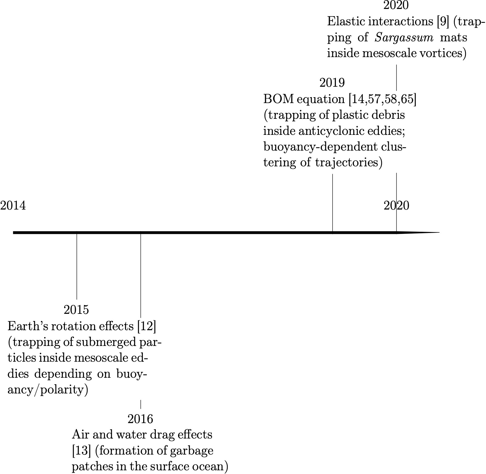
Figure 1: Timeline of oceanographic extensions of the Maxey–Riley equation.

The overview starts with a review of the original Maxey–Riley equation (Sec. 2). This is followed by a review of a geophysical adaptation and a concrete oceanographic application (Sec. 3). The BOM equation is reviewed in Sec. 4, which includes results from field and laboratory experiments in support of its validity. Section 5 is dedicated to review an extension of the BOM equation to model the motion of elastic networks of floating inertial particles that emulate rafts of Sargassum. Concluding remarks on aspects that still need to be addressed to expand the applicability of the Maxey–Riley framework to oceanography are finally made in Sec. 6.

2 The original Maxey–Riley equation

As already noted, the study of the motion of inertial (i.e., buoyant, finite-size) particles was pioneered by Sir George Stokes Stokes (1851), who solved the linearized Navier–Stokes equations for the oscillatory motion of a small solid sphere (pendulum) immersed in a fluid at rest. This was followed by the efforts of Basset (1888), Boussinesq (1885), and Oseen (1927) to model a solid sphere settling under gravity, also in a quiescent fluid. Tchen (1947) extended these efforts to model motion in nonuniform unsteady flow by writing the resulting equation, known as the BBO equation, on a frame of reference moving with the fluid. Several corrections to the precise form of the forces exerted on the particle due to the solid–fluid interaction were made along the years (e.g., Corrsin and Lumely, 1956). The now widely accepted form of the forces was derived by Maxey and Riley (1983) from first principles, following an approach introduced by Riley (1971). The resulting equation, with a correction made by Auton et al. (1988), is widely referred to as the Maxey–Riley equation. A similar equation was derived, independently and nearly simultaneously, by Gatignol (1983). Michaelides (1997) and Cartwright et al. (2010) review the Maxey–Riley equation in some detail.

2.1 Setup

Let $x=(x^{1},x^{2})$ be position on an open domain of $\mathbb{R}^{2}$. As our ultimate interest is in geophysical applications, this domain is actually assumed to lie on a horizontal plane, i.e., perpendicular to the local gravity direction. Let $t\in\mathbb{R}$ be time. Let $v_{\mathrm{f}}(x,t)$ be the velocity of a fluid of constant density $\rho_{\mathrm{f}}$ and dynamic viscosity $\mu_{\mathrm{f}}$. Consider a solid sphere immersed in the fluid. Let $a$ be its radius, which is assumed to be small compared to any relevant length scales of the problem, and $\rho_{\mathrm{p}}=\operatorname{const}$ its density. Let

$$\delta:=\frac{\rho_{\mathrm{f}}}{\rho_{\mathrm{p}}},$$ (1)

which will be referred to as buoyancy. Indeed, particles that are lighter (resp., heavier) than the carrying fluid are characterized by $\delta>1$ (resp., $\delta<1$). We will restrict attention in this section to the case $\delta\approx 1$, so the vertical motion of the particle can be neglected (rapid, small-scale three-dimensional motions that can alter this balance are not considered here as the interest relies on slow, large-scale geophysical flow motions, which are essentially two dimensional).

2.2 Forces and the resulting equation

The Maxey–Riley equation is a classical mechanics Newton’s 2nd law with several forces describing the motion of a small solid sphere immersed in the unsteady nonuniform flow of a homogeneous, viscous fluid. As such, it represents an ordinary differential equation that provides an approximation to the motion of inertial particles. Its exact motion is controlled by the Navier–Stokes equation with moving boundaries. This is necessarily described by partial differential equations, which much more difficult to solve and analyze than an ordinary differential equation.

The Maxey–Riley equation includes several forcing terms which prevent inertial particles from adapting their velocities to instantaneous changes in the carrying flow field. Normalized by particle mass $m_{\mathrm{p}}=\frac{4}{3}\pi a^{3}\rho_{\mathrm{p}}$ the relevant forces for the horizontal motion are:

1. the flow force exerted on the particle by the undisturbed fluid:

   $$F_{\mathrm{flow}}=\frac{m_{\mathrm{f}}}{m_{\mathrm{p}}}\frac{\operatorname{D}\!{v_{\mathrm{f}}}}{\operatorname{D}\!{t}}$$ (2)

   where $m_{\mathrm{f}}=\frac{4}{3}\pi a^{3}\rho_{\mathrm{f}}$ is the mass of the displaced fluid and $\smash{\frac{\operatorname{D}\!{}}{\operatorname{D}\!{t}}}v_{\mathrm{f}}$ is the fluid velocity’s material derivative, namely, $\smash{\frac{\operatorname{D}\!{}}{\operatorname{D}\!{t}}}v_{\mathrm{f}}=\smash{\big{[}\frac{\operatorname{d}\!{}}{\operatorname{d}\!{t}}v_{\mathrm{f}}(x,t)\big{]}_{x=X_{\mathrm{f}}(t)}}=\partial_{t}v_{\mathrm{f}}+(\nabla v_{\mathrm{f}})v_{\mathrm{f}}$, where $x=X_{\mathrm{f}}(t)$ is a fluid trajectory;

2. the added mass force resulting from part of the fluid moving with the particle:

   $$F_{\mathrm{mass}}=\frac{\frac{1}{2}m_{\mathrm{f}}}{m_{\mathrm{p}}}\left(\frac{\operatorname{D}\!{v_{\mathrm{f}}}}{\operatorname{D}\!{t}}-\dot{v}_{\mathrm{p}}\right)$$ (3)

   where $\dot{v}_{\mathrm{p}}$ is the acceleration of an inertial particle with trajectory $x=X_{\mathrm{p}}(t)$, i.e., $\dot{v}_{\mathrm{p}}=\smash{\frac{\operatorname{d}\!{}}{\operatorname{d}\!{t}}\left[v_{\mathrm{p}}(x,t)\right]_{x=X_{\mathrm{p}}(t)}}=\partial_{t}v_{\mathrm{p}}$ where $v_{\mathrm{p}}=\partial_{t}X_{\mathrm{p}}=\dot{x}$ is the inertial particle velocity;

3. the lift force, which arises when the particle rotates as it moves in a (horizontally) sheared flow,

   $$F_{\mathrm{lift}}=\frac{\frac{1}{2}m_{\mathrm{f}}}{m_{\mathrm{p}}}\omega_{\mathrm{f}}J(v_{\mathrm{f}}-v_{\mathrm{p}}),$$ (4)

   where $\omega_{\mathrm{f}}=\partial_{1}v^{2}_{\mathrm{f}}-\partial_{2}v^{1}_{\mathrm{f}}$ is the (vertical) vorticity of the fluid and

   $$J:=\begin{pmatrix}0&-1\\ 1&0\end{pmatrix};$$ (5)

4. the drag force caused by the fluid viscosity,

   $$F_{\mathrm{drag}}=\frac{12\mu_{\mathrm{f}}\frac{A_{\mathrm{f}}}{\ell_{\mathrm{f}}}}{m_{\mathrm{p}}}(v_{\mathrm{f}}-v_{\mathrm{p}})$$ (6)

   where $A_{\mathrm{f}}$ ($=\pi a^{2}$) is the projected area of the particle and $\ell_{\mathrm{f}}$ ($=2a$) is the characteristic projected length.

The Maxey–Riley equation, $\dot{v}_{\mathrm{p}}=F_{\mathrm{flow}}+F_{\mathrm{mass}}+F_{\mathrm{lift}}+F_{\mathrm{drag}}$, reads

$$\dot{v}_{\mathrm{p}}+\left(\tfrac{1}{2}R\omega_{\mathrm{f}}J+\frac{\operatorname{Id}}{\tau}\right)v_{\mathrm{p}}=\tfrac{3}{2}R\frac{\operatorname{D}\!{v_{\mathrm{f}}}}{\operatorname{D}\!{t}}+\left(\tfrac{1}{2}R\omega_{\mathrm{f}}J+\frac{\operatorname{Id}}{\tau}\right)v_{\mathrm{f}},$$ (7)

where

$$R:=\frac{2\delta}{2+\delta},\quad\tau:=\tfrac{2}{3}R^{-1}\cdot\frac{a^{2}\rho_{\mathrm{f}}}{3\mu_{\mathrm{f}}}.$$ (8)

Here $\tau$ is the inertial particle’s response time to the medium or Stokes’ time. Note that $0\leq R<2$ with $R>\smash{\frac{2}{3}}$ (resp., $R<\smash{\frac{2}{3}}$) characterize light (resp., heavy) particles.

Remark 1

A pertinent question is whether the fluid particle equation $\dot{x}=v_{\mathrm{f}}$ is recovered from (7) when $R=\smash{\frac{2}{3}}$ and $\tau=0$. The answer to this question is affirmative, essentially. Yet it requires elaboration, provided in the next section, as (7) becomes singular at $\tau=0$.

Remark 2

Except for the lift force, due to Auton (1987), the forces just described are included in the paper by Maxey and Riley (1983), yet with a different form of the added mass term, which corresponds to the correction due to Auton et al. (1988). The particular form of the lift force above is found in (Montabone, 2002, Ch. 4); similar forms are considered in Henderson et al. (2007) and Sapsis et al. (2011). A condition for the validity of the lift force is (Auton, 1987; Auton et al., 1988)

$$\frac{|\omega_{\mathrm{f}}|a}{|v_{\mathrm{f}}-v_{\mathrm{p}}|}\ll 1.$$ (9)

Remark 3

The Maxey–Riley equation (7) was derived under the assumption that the particle Reynolds number

$$\operatorname{Re_{p}}:=\frac{V_{\mathrm{slip}}\cdot\ell_{\mathrm{f}}}{\mu_{\mathrm{f}}/\rho_{\mathrm{f}}}\ll 1,$$ (10)

where $V_{\mathrm{slip}}$ is a measure of the difference between $v_{\mathrm{p}}$ and $v_{\mathrm{f}}$. We will see that this is indeed well satisfied for sufficiently small particles since in that case $v_{\mathrm{p}}$ is asymptotically close to $v_{\mathrm{f}}$.

Remark 4

The general form of the drag force (e.g., Kundu et al. (2012)) per unit particle mass is:

$$F_{\mathrm{drag}}=\frac{\tfrac{1}{2}\rho_{\mathrm{f}}C_{\mathrm{D}}A_{\mathrm{f}}}{m_{\mathrm{p}}}|v_{\mathrm{f}}-v_{\mathrm{p}}|(v_{\mathrm{f}}-v_{\mathrm{p}}).$$ (11)

A particle in a flow in Stokes’ regime, for which $\mathrm{Re_{p}}<1$, is characterized by a drag coefficient of the form

$$C_{\mathrm{D}}=\frac{24}{\mathrm{Re_{p}}}.$$ (12)

Plugging $C_{\mathrm{D}}=24/\mathrm{Re_{p}}$ in the general drag formula (11), one gets, upon setting $V_{\mathrm{slip}}=|v_{\mathrm{f}}-v_{\mathrm{p}}|$,

$$F_{\mathrm{drag}}=\frac{\tfrac{1}{2}\rho_{\mathrm{f}}\frac{24}{\mathrm{Re_{p}}}A_{\mathrm{f}}}{m_{\mathrm{p}}}|v_{\mathrm{f}}-v_{\mathrm{p}}|(v_{\mathrm{f}}-v_{\mathrm{p}})=\frac{12\mu_{\mathrm{f}}\frac{A_{\mathrm{f}}}{\ell_{\mathrm{f}}}}{m_{\mathrm{p}}}(v_{\mathrm{f}}-v_{\mathrm{p}}).$$ (13)

Remark 5

In writing the Maxey–Riley equation (7) we have ignored the Basset–Boussinesq history or memory term, which is an integral term that makes the equation a fractional differential equation Daitche and Tél (2011, 2014); Langlois et al. (2015). This may be (has been) neglected under low recurrence time grounds Sudharsan et al. (2016). It has been also noted Daitche and Tél (2011) that it mainly tends to slow down the inertial particle motion without changing its qualitative dynamics fundamentally. However, the effects of the memory terms remain the subject of active research Olivieri et al. (2014); Prasath et al. (2019); Haller (2014). We have also ignored so-called Faxen corrections (terms of the form $a^{2}\nabla^{2}v_{\mathrm{f}}$) in the added mass and drag forces; this is much easier to justify.

2.3 Slow manifold reduction

Because of the small-particle-size assumption involved in the derivation of the Maxey–Riley equation, it is natural to investigate its asymptotic behavior when $\tau=O(\varepsilon)$ as $\varepsilon\to 0$, where $0\leq\varepsilon\ll 1$ is a parameter that we will use to measure smallness (of any nature) throughout this paper (in this case it can be interpreted as a Stokes number (Haller and Sapsis, 2008)). In this limit, the Maxey–Riley equation (7) involves a fast variable, $v_{\mathrm{p}}$, changing at $O(\varepsilon^{-1})$ speed, and a slow variable, $x$, changing at $O(1)$ speed, which makes (7) a singular perturbation problem. This can be seen by putting (7) in system form, viz.,

$$\dot{x}=v_{\mathrm{p}},\quad\dot{v}_{\mathrm{p}}=\frac{v_{\mathrm{f}}-v_{\mathrm{p}}}{\tau}+\tfrac{3}{2}R\frac{\operatorname{D}\!{v_{\mathrm{f}}}}{\operatorname{D}\!{t}}+\tfrac{1}{2}R\omega_{\mathrm{f}}J\left(v_{\mathrm{f}}-v_{\mathrm{p}}\right),\quad\dot{t}=1.$$ (14)

Changing $t$ by the fast time $s=\frac{t-t_{0}}{\varepsilon}$ Haller and Sapsis (2008), system (14) recasts as

$$x^{\prime}=\varepsilon v_{\mathrm{p}},\quad v^{\prime}_{\mathrm{p}}=\frac{v_{\mathrm{f}}-v_{\mathrm{p}}}{\tau/\varepsilon}+\tfrac{3}{2}R\frac{\operatorname{D}\!{v_{\mathrm{f}}}}{\operatorname{D}\!{t}}+\tfrac{1}{2}R\omega_{\mathrm{f}}J\left(v_{\mathrm{f}}-v_{\mathrm{p}}\right),\quad t^{\prime}=\varepsilon,$$ (15)

where ${}^{\prime}=\frac{\operatorname{d}\!{}}{\operatorname{d}\!{s}}$. There are two distinguished limiting behaviors for the above systems. Setting $\tau=0$ in the fast system (15),

$$x^{\prime}=0,\quad v^{\prime}_{\mathrm{p}}=v_{\mathrm{f}}-v_{\mathrm{p}},\quad t^{\prime}=0,$$ (16)

from which one obtains that $x$ and $t$ do not change, yet the motion is accelerated. This physically absurd situation however is consistent with $v_{\mathrm{p}}$ being the fast variable and $x$ and $t$ the slow variables. The corresponding limit of the slow system (14),

$$\dot{x}=v_{\mathrm{p}},\quad 0=v_{\mathrm{f}}-v_{\mathrm{p}},\quad\dot{t}=1,$$ (17)

gives the motion on

$$M_{0}:=\big{\{}(x,v_{\mathrm{p}},t):v_{\mathrm{p}}=v_{\mathrm{f}}(x,t)\big{\}},$$ (18)

which is the set of equilibria of (16). Thus while (16) has a large set of equilibria on which the motion is trivial, (17) blows the flow on this set up to produce nontrivial behavior, yet leaving the flow off the set undetermined. This makes the resolution of (14) a singular perturbation problem.

The goal of the geometric singular perturbation theory (GSPT) of Fenichel (1979) (cf. the lecture notes of Jones (1995) for additional insight), extended to nonautonomous systems by Haller and Sapsis (2008), is to capture the fast and slow aspects of the motion in systems like (14) simultaneously. This is accomplished in the case of (14) by examining the motion for $\tau=O(\varepsilon)$ as $\varepsilon\to 0$ as follows.

Assume that $v_{\mathrm{f}}(x,t)$ is smooth in each of its arguments. Then $M_{0}$ represents a 3-dimensional, invariant, globally attracting, normally hyperbolic manifold for (16) Fenichel (1972). Indeed, $M_{0}$ is filled with equilibria of (16), whose linearization at each point on $M_{0}$ has 3 null eigenvalues, with corresponding neutral eigenvectors tangent to $M_{0}$, and 2 eigenvalues equal to $-1$, with corresponding contracting eigenvectors such that $(x,t)=\operatorname{const}$. Since tangencies are ruled out by the smoothness assumption on $v_{\mathrm{f}}$, this guarantees that contraction occurs in the normal direction to $M_{0}$ exclusively. More explicitly, integrating (16),

$$x=x_{0},\quad v_{\mathrm{p}}=v_{\mathrm{f}}(x_{0},0)+\big{(}v_{\mathrm{p}}(0)-v_{\mathrm{f}}(x_{0},0)\big{)}\cdot\operatorname{e}^{-s},\quad t=t_{0},$$ (19)

which shows that any initial condition of (16) has its $\omega$-limit in $M_{0}$ and that the normal projection of a normal perturbation to $M_{0}$ decays under the (linearized) flow as $\operatorname{e}^{-s}$, while the tangential projection grows as $1-\operatorname{e}^{-s}$, except at critical points where it vanishes.

Then nonautonomous GSPT guarantees the existence of a locally invariant (i.e., up to trajectories leaving through the boundary), globally attracting, normally hyperbolic manifold

$$M_{\tau}:=\Big{\{}(x,v_{\mathrm{p}},t):v_{\mathrm{p}}=v_{\mathrm{f}}(x,t)+\sum_{1}^{r}\tau^{n}v_{n}(x,t)+O(\varepsilon^{r+1})\Big{\}}$$ (20)

for (14)—or (15)—when $\tau=O(\varepsilon)$ as $\varepsilon\to 0$, called a slow manifold, which is $O(\varepsilon)$-close to the critical manifold $M_{0}$ and $C^{r}$-diffeomorphic to it for any $r<\infty$. Restricted to $M_{\tau}$, (14) slowly varies while controlling the motion off $M_{\tau}$ as follows. When $\tau\propto\varepsilon=0$, each point off $M_{0}$ belongs to the stable manifold of $M_{0}$, which is foliated by its distinct stable fibers (stable manifolds of points on $M_{0}$) satisfying $(x,t)=\operatorname{const}$. The stable manifold of $M_{0}$ and its stable fibers perturb along with $M_{0}$. As a result, for $\tau=O(\varepsilon)$ as $\varepsilon\to 0$ each point off the slow manifold $M_{\tau}$ is connected to a point on $M_{\tau}$ by a fiber in the sense that it follows a trajectory that approaches its partner on $M_{\tau}$ exponentially fast in time. The geometry of these results is illustrated in Fig. 2.

The functions $v_{n}(x,t)$ that determine $M_{\tau}$ are obtained by substituting the asymptotic expansion in (20) in the second equation of (14) with the first equation in mind, which tells that $\dot{\varphi}=\partial_{t}\varphi+(\nabla\varphi)v_{\mathrm{p}}$ for any function $\varphi(x,t)$, and then equating terms of like order of $\varepsilon$. This gives (cf. App. C of Ref. Beron-Vera et al., 2019)

$$v_{1} =\big{(}\tfrac{3}{2}R-1\big{)}\frac{\operatorname{D}\!{v_{\mathrm{f}}}}{\operatorname{D}\!{t}}$$ (21)

$$v_{n} =-\tfrac{1}{2}R\omega Jv_{n-1}-\frac{\operatorname{D}\!{}}{\operatorname{D}\!{t}}v_{n-1}-(\nabla v)v_{n-1}-\sum_{m=1}^{n-2}(\nabla v_{m})v_{n-m-1},\quad n\geq 2.$$ (22)

One then finds that

$$\dot{x}=v_{\mathrm{p}}=v_{\mathrm{f}}+\tau\big{(}\tfrac{3}{2}R-1\big{)}\frac{\operatorname{D}\!{v_{\mathrm{f}}}}{\operatorname{D}\!{t}}$$ (23)

describes, with an $O(\varepsilon^{2})$ error, the asymptotic dynamics of the Maxey–Riley equation on the slow manifold $M_{\tau}$ in the form of a regular perturbation problem.

We will refer (23) to as the reduced Maxey–Riley equation. This reduced equation coincides with that derived in Haller and Sapsis (2008) ignoring the lift term, which makes a higher-order contribution in $\varepsilon$ to $M_{\tau}$—it appears at $O(\varepsilon^{2})$; cf. (22). The special case of a steady cellular carrying flow, also without lift term, was considered by Rubin et al. (1995), who first reported an analysis of the Maxey–Riley equation using (autonomous) GSPT.

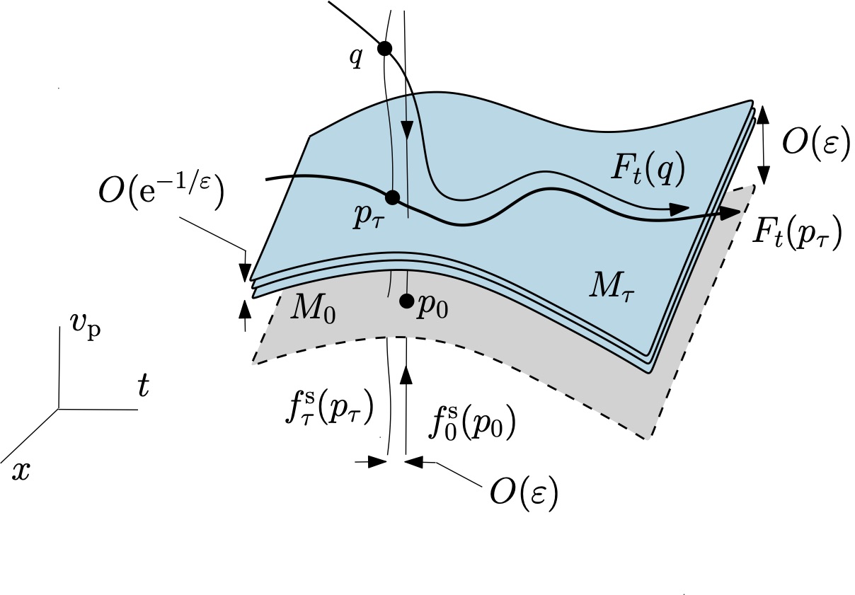
Figure 2: Geometry of the Maxey–Riley equation (7). In the $\tau=0$ limit the equation has a globally attracting, normally hyperbolic invariant manifold, $M_{0}$, filled with equilibria. For $\tau=O(\varepsilon)$ as $\varepsilon\to 0$, there exists a unique up to an error of $O(\smash{\mathrm{e}^{-1/\varepsilon}})$, locally invariant, globally attracting manifold $M_{\tau}$, which lies at an $O(\varepsilon)$ distance to $M_{0}$ and is diffeomorphic to it. Restricted to $M_{\tau}$, the Maxey–Riley equation slowly varies while controlling the motion off $M_{\tau}$ as follows. When $\tau=0$, each point off $M_{0}$ belongs to the stable manifold of $M_{0}$, which is foliated by its distinct stable fibers or stable manifolds of points $p_{0}$ on $M_{0}$, $f_{0}^{s}(p_{0})$, satisfying $(x,t)=\operatorname{const}$. The stable manifold of $M_{0}$ and its stable fibers perturb along with $M_{0}$. Consequently, for $\tau=O(\varepsilon)$ each point $q$ off the slow manifold $M_{\tau}$ is connected to a point $p_{\tau}$ on $M_{\tau}$ by a fiber $f_{\tau}^{s}(p_{\tau})$ in the sense that it follows a trajectory $F_{t}(q)$ that converges to its partner $F_{t}(p_{\tau})$ on $M_{\tau}$ exponentially fast in time.

Remark 6

The slow manifold is not unique. There typically is a family of slow manifolds with members lying at an $\smash{O(\mathrm{e}^{-1/\varepsilon})}$ distance from one another Fenichel (1979). On the other hand, rapid changes in the carrying fluid velocity $v_{\mathrm{f}}$ will lead to rapid changes in $M_{\tau}$, thereby restricting its ability to absorb solutions over finite time. In other words, the convergence to $M_{\tau}$ may not be monotone Haller and Sapsis (2008).

Remark 7

As a 2-dimensional system, the reduced Maxey–Riley equation (23) is numerically less expensive to solve than the full Maxey–Riley equation (7), which is 4-dimensional. As such, it requires specification of initial positions only, rather than initial positions and velocities, which are generally not available. Also, unlike the full equation, the reduced equation is not subjected to numerical instability in backward time integration Haller and Sapsis (2008), which is useful in source inversion. Furthermore, as we will see, it provides insight that is difficult to be attained using the full Maxey–Riley equation.

Remark 8

The slow manifold $M_{\tau}$ (20) and the restriction of the Maxey–Riley equation to $M_{\tau}$ (23) formally satisfy the definition of inertial manifold and inertial equation, respectively, developed for the study of attractors in infinite-dimensional dynamical systems Temam (1990). In such systems, actual attractors are hard to compute and are generally not even manifolds. The inertial manifold is easier to compute, smooth, and contains the attractor. It is unclear to the author why the term “inertial” is used to denote such manifolds. Here “inertia” refers to resistance of an object to a change in its velocity.

2.4 Neutrally buoyant particles

The neutrally buoyant case $\delta=1$ or, equivalently, $R=\smash{\frac{2}{3}}$ deserves a separate discussion. The results above imply that neutrally buoyant particle motion synchronizes exponentially fast with Lagrangian particle motion when particles are sufficiently small, i.e., $\tau=O(\varepsilon)$. Indeed, on the slow manifold $\dot{x}=v_{\mathrm{p}}=v_{\mathrm{f}}$ with an $O(\varepsilon^{2})$ error. However, Babiano et al. (2000) noted that, in the case with no lift force, the manifold

$$N:=\big{\{}(x,v_{\mathrm{p}},t):v_{\mathrm{p}}=v_{\mathrm{f}}(x,t)\big{\}},$$ (24)

while invariant for any $\tau$, may become unstable for $\tau$ large. The neutral manifold $N$ coincides with the critical manifold $M_{0}$ in (18). But this is not true in the ocean adaption(s) of the Maxey–Riley equation discussed below, so is appropriate to use different labels for these two manifolds.

The invariance of $N$ holds even with lift term present (Beron-Vera et al., 2019, App. B), as one finds by writing the Maxey–Riley equation (7) with $R=\smash{\frac{2}{3}}$ following Babiano et al. (2000) as

$$\dot{y}=Ay,\quad y:=v_{\mathrm{p}}-v_{\mathrm{f}}\quad A:=-\big{(}\nabla v_{\mathrm{f}}+\tfrac{1}{3}\omega_{\mathrm{f}}J+\tau^{-1}\operatorname{Id}\big{)}.$$ (25)

Here $\dot{v}_{\mathrm{f}}=\partial_{t}v_{\mathrm{f}}+(\nabla v_{\mathrm{f}})v_{\mathrm{p}}$ is the total derivative of $v$ taken along an inertial particle trajectory, satisfying $\dot{x}=v_{\mathrm{p}}$. Clearly $y=0$ trivially solves $\dot{y}=Ay$. From this it follows that $N$ is invariant for any $\tau$.

The possibility of growing perturbations off $N$ follows from inspecting the sign of the instantaneous stability indicator, discussed by Sapsis and Haller (2008),

$$\Lambda(x_{0},t_{0}):=\lim_{t\to t_{0}}\frac{2}{t-t_{0}}\log||P_{t_{0}}^{t}||_{2},$$ (26)

where $P_{t_{0}}^{t}$ is the fundamental matrix solution of (25). Taylor expanding $P_{t_{0}}^{t}$,

$$(||P_{t_{0}}^{t}||_{2})^{2}=1-2\min\operatorname{spec}(S(x_{0},t_{0})+\tau^{-1}\operatorname{Id})\cdot(t-t_{0})+O((t-t_{0})^{2}),$$ (27)

where $S:=\smash{\frac{\nabla v+(\nabla v)^{\top}}{2}}$ is the strain-rate tensor, and $\log\left(1+\smash{\sum_{1}^{\infty}}c_{n}\varepsilon^{n}\right)=c_{1}\varepsilon+O(\varepsilon^{2})$, it follows that

$$\Lambda(x_{0},t_{0})=-2\min\operatorname{spec}(S(x_{0},t_{0})+\tau^{-1}\operatorname{Id})$$ (28)

(cf. App. B of Ref. Beron-Vera et al., 2019, for deatils). Replacing $(x_{0},t_{0})$ with $(x(t),t)$ one concludes that instantaneous divergence away from $N$ will necessarily take place where

$$\tau>\frac{2}{\sqrt{S_{\mathrm{n}}^{2}+S_{\mathrm{s}}^{2}}-\nabla\cdot v}.$$ (29)

Here $S_{\mathrm{n}}:=\partial_{1}v_{\mathrm{f}}^{1}-\partial_{2}v_{\mathrm{f}}^{2}$ and $S_{\mathrm{s}}:=\partial_{2}v_{\mathrm{f}}^{1}+\partial_{1}v_{\mathrm{f}}^{2}$ are normal and shear strain components, respectively. Condition (29) reduces to $\tau>1/\sqrt{|\det S|}$ in the (geophysically relevant) incompressible case $\nabla\cdot v=0$. This coincides with that one obtained in Sapsis and Haller (2008) ignoring the lift force, which is seen to play no role in setting the local instability of $N$.

A sufficient condition for global attractivity on $N$ is provided by the violation of (29) everywhere as it follows by noting that

$$|y(t)|\leq|y(t_{0})|\mathrm{e}^{-\textstyle{\int_{t_{0}}^{t}}\min\operatorname{spec}(S(x(s),s)+\tau^{-1}\operatorname{Id})\operatorname{d}\!{s}},$$ (30)

where $y^{\top}Ay\leq\smash{\frac{1}{2}}\max\operatorname{spec}(A+A^{\top})\cdot|y|^{2}=-\min\operatorname{spec}\big{(}S+\tau^{-1}\operatorname{Id}\big{)}\cdot|y|^{2}$ was taken into account (Beron-Vera et al., 2019, App. B).

Remark 9

It is important to realize that for $(y_{0},x_{0})$ given, convergence on $N$ does not imply convergence on a fluid trajectory starting on $x_{0}$. Consider $v_{\mathrm{f}}=V=\operatorname{const}$. This implies that $\omega=0$. It readily follows that $y=y_{0}\smash{\mathrm{e}^{-t/\tau}}$ and $x=x_{0}+Vt+\tau y_{0}(1-\smash{\mathrm{e}^{-t/\tau}})$. Note that while $y\to 0$ as $t\to\infty$, $x\to x_{0}+Vt+\tau y_{0}$, when the fluid trajectory starting from $x_{0}$ is $x_{0}+Vt$. Clearly, coincidence is expected only when the neutrally buoyant particle is sufficiently small, i.e., $\tau=O(\varepsilon)$, consistent with $N$ lying at $O(\varepsilon^{2})$ distance to $M_{\tau}$, which attracts all solutions in that limit.

Remark 10

It turns out that (29) is also a necessary condition for the instability of perturbations off the slow manifold $M_{\tau}$ given in (20), i.e., without the neutrally buoyant particle constraint. This follows from the local instability analysis of an arbitrary invariant manifold developed by Haller and Sapsis (2010). The main result of that work is the derivation of a local stability indicator, called normal infinitesimal Lyapunov exponent or NILE, which is related to the instantaneous stability indicator (26). For a system of the form

$$\dot{x}=f(x,y,t),\quad\dot{y}=g(x,y,t),$$ (31)

the NILE for a perturbation off a general invariant manifold of graph form,

$$M=\{(x,y,t):y=h(x,t)\},$$ (32)

is given by

$$\sigma(x,t)=\tfrac{1}{2}\max\operatorname{spec}\big{(}\Gamma(x,t)+\Gamma(x,t)^{\top}\big{)}$$ (33)

where

$$\Gamma(x,t):=(\partial_{y}g-\partial_{x}h\partial_{y}f)|_{y=h(x,t)}.$$ (34)

In other words, the manifold $M$ becomes locally repelling in $(x,t)$ regions where the NILE is positive. For a perturbation off slow manifold $M_{\tau}$ of the Maxey–Riley equation (7), $\sigma(x,t)=-\min\operatorname{spec}\smash{\big{(}S(x,t)+\tau^{-1}\operatorname{Id}\big{)}}+O(\varepsilon)$, whose lowest-order contribution is positive for $(x,t)$ where (29) holds. It should be realized that this result does not contradict the nonautonomous GSPT result on the global attractivity of $M_{\tau}$, which is an asymptotic result. It is consistent with Remark 6 on the possible nonmonotonic convergence to $M_{\tau}$ Haller and Sapsis (2008).

3 Geophysical extension of the original Maxey–Riley equation

As a first step toward preparing for oceanographic applications of the Maxey–Riley equation, we need to move away from the laboratory frame, taking into account the effects of the rotation of the Earth and its curvature. The adaption that follows actually applies more widely to geophysical flows, such as Earth atmospheric flows and possibly also planetary atmospheric flows. Indeed, this adaptation has been suitable to provide insight into aspects of inertial motion in the ocean Beron-Vera et al. (2015); Haller et al. (2016) and also in the stratosphere Provenzale (1999).

3.1 The Coriolis force

Let $a_{\odot}$ be the Earth’s radius, and consider the rescaled longitude ($\lambda$) and latitude ($\vartheta$) coordinates:

$$x^{1}=(\lambda-\lambda_{0})\cdot a_{\odot}\cos\vartheta_{0},\quad x^{2}=(\vartheta-\vartheta_{0})\cdot a_{\odot},$$ (35)

where $(\lambda_{0},\vartheta_{0})$ is a reference location on the planet’s surface. Consider the following geometric coefficients Ripa (1997a):

$$\gamma_{\odot}:=\sec\vartheta_{\odot}\cos\vartheta,\quad\tau_{\odot}:=a^{-1}_{\odot}\tan\vartheta.$$ (36)

The (horizontal) velocity of a fluid particle and its acceleration as measured by a terrestrial observer are Ripa (1997a); Beron-Vera (2003)

$$v_{\mathrm{f}}=m_{\odot}\dot{x},\quad m_{\odot}:=\begin{pmatrix}\gamma_{\odot}&0\\ 0&1\end{pmatrix},\quad a_{\mathrm{f}}=\dot{v}_{\mathrm{f}}+(f+\tau_{\odot}v_{\mathrm{f}}^{1})Jv_{\mathrm{f}},$$ (37)

respectively, where $f:=2\Omega\sin\vartheta$ is the Coriolis “parameter.”

A very enlightening way to derive the formula for the acceleration is from Hamilton’s principle, where the Lagrangian is written by an observer standing on a fixed frame but with the coordinates related to those rotating with the planet. This way the only force acting on the particle (in the absence of any other forces) is the gravitational one. This is in essence what Pierre Simon de Laplace (1749–1827) did to derive his theory of tides and at the same time discover the Coriolis force over a quarter of a century before Gaspard Gustave de Coriolis (1792–1843) was born Ripa (1995, 1997b, 1997a).

Remark 11

Indeed, for an observer standing on a fixed frame, the only force acting on a free particle on the assumed smooth, frictionless surface, $S$, of the Earth is the gravitational force. Thus, on $S$, we must have $V+V_{\mathrm{C}}=0$ (without loss of generality) where $V$ and $V_{\mathrm{C}}$ are gravitational and centrifugal potentials, respectively Ripa (1997a); Beron-Vera (2003). The centrifugal potential is easy to express: $V_{\mathrm{C}}=\smash{\tfrac{1}{2}a_{\odot}^{2}\Omega^{2}\cos^{2}\vartheta}$. In turn, the kinetic energy of the particle as measured by the fixed observer, $T:=\smash{\tfrac{1}{2}a_{\odot}^{2}}(\cos^{2}\vartheta(\dot{\vartheta}+\Omega)^{2}+\dot{\vartheta}^{2})$. Using Pedro Ripa’s convenient trick Ripa (1997a) to augment the number of generalized coordinates from $(x^{1},y^{1})$ to $(x^{1},x^{2},v^{1}=\gamma_{\odot}\dot{x}^{1},v^{2}=\dot{x}^{2})$, the Lagrangian, $L:=T-V\equiv\gamma_{\odot}\dot{x}^{1}\smash{\big{(}v^{1}+\tfrac{1}{2}\tau_{\odot}^{-1}f\big{)}}+\dot{x}^{2}v^{2}-\smash{\tfrac{1}{2}\big{(}(v^{1})^{2}+(v^{2})^{2}\big{)}}$, which leads (directly) to a motion equation equation in system form, viz., $\dot{x}=m_{\odot}^{-1}v$ and $\dot{v}+(f+\tau_{\odot}v^{1})Jv=0$; cf. (37).

By a similar token, the fluid’s Eulerian acceleration takes the form

$$\frac{\operatorname{D}\!{v_{\mathrm{f}}}}{\operatorname{D}\!{t}}+(f+\tau_{\odot}v_{\mathrm{f}}^{1})Jv_{\mathrm{f}},$$ (38)

where

$$\frac{\operatorname{D}\!{v_{\mathrm{f}}}}{\operatorname{D}\!{t}}=\partial_{t}v_{\mathrm{f}}+(\nabla v_{\mathrm{f}})\dot{x}=\partial_{t}v_{\mathrm{f}}+(\gamma_{\odot}^{-1}\partial_{1}v_{\mathrm{f}})v_{\mathrm{f}}^{1}+(\partial_{2}v_{\mathrm{f}})v_{\mathrm{f}}^{2}.$$ (39)

The vorticity,

$$\omega_{\mathrm{f}}=\gamma_{\odot}^{-1}\partial_{1}v_{\mathrm{f}}^{2}-\gamma_{\odot}^{-1}\partial_{2}(\gamma_{\odot}v_{\mathrm{f}}^{1})=\gamma_{\odot}^{-1}\partial_{1}v_{\mathrm{f}}^{2}-\partial_{2}v_{\mathrm{f}}^{1}+\tau_{\odot}v_{\mathrm{f}}^{1}$$ (40)

as it follows from its definition, $\omega:=\smash{\lim_{\Delta x^{1}\Delta x^{2}\to 0}}\smash{\frac{1}{\gamma_{\odot}\Delta x^{1}\Delta x^{2}}}\smash{\oint}(\gamma_{\odot}v_{\mathrm{f}}^{1}\operatorname{d}\!{x^{1}}+v_{\mathrm{f}}^{2}\operatorname{d}\!{x^{2}})$, and noting that $\gamma_{\odot}^{\prime}(x^{2})/\gamma_{\odot}(x^{2})=-\tau_{\odot}(x^{2})$.

A version of the Maxey–Riley equation that is suitable for geophysical applications follows by replacing $\dot{v}_{\mathrm{p}}$ in the original equation (7) by (37) with $v_{\mathrm{f}}=v_{\mathrm{p}}$ and $\smash{\frac{\operatorname{D}\!{}}{\operatorname{D}\!{t}}}v_{\mathrm{f}}$ by (38), viz.,

$$\dot{v}_{\mathrm{p}}+\left(\left(f_{\mathrm{p}}\!+\!\tfrac{1}{2}R\omega_{\mathrm{f}}\right)J\!+\!\frac{\operatorname{Id}}{\tau}\right)v_{\mathrm{p}}=\tfrac{3}{2}R\frac{\operatorname{D}\!{v_{\mathrm{f}}}}{\operatorname{D}\!{t}}+\left(\tfrac{3}{2}R\left(f_{\mathrm{f}}\!+\!\tfrac{1}{3}\omega_{\mathrm{f}}\right)J\!+\!\frac{\operatorname{Id}}{\tau}\right)v_{\mathrm{f}},$$ (41)

where $f_{\boldsymbol{\cdot}}:=f+\tau_{\odot}v^{1}_{\boldsymbol{\cdot}}$. A convenient simplification which treats $(x^{1},x^{2})$ as if it were Cartesian position as in our original setting is defined by $\gamma_{\odot}=1$, $\tau_{\odot}=0$, and $f_{\boldsymbol{\cdot}}=f=f_{0}+\beta x^{2}$. This is called a $\beta$-plane approximation, valid for $|x^{2}|\ll a_{\odot}$, with caveats Ripa (1997a).

Remark 12

We will herein make use of the $\beta$-plane approximation for simplicity of exposition, with $x^{1}$ (resp., $x^{2}$) Cartesian and pointing eastward (resp., northward). Results due to Coriolis effects do not change when working on full spherical geometry.

Remark 13

A version of the Maxey–Riley equation with Coriolis force appears in Provenzale (1999). That version, however, as also includes the centrifugal force, which is exactly balanced by the gravitational force on a plane tangent to the Earth’s surface.

Application of nonautonomous GSPT analysis when $\tau=O(\varepsilon)$ as $\varepsilon\to 0$ leads to the following reduced equation on the slow manifold:

$$\dot{x}=v_{\mathrm{p}}=v_{\mathrm{f}}+\tau\big{(}\tfrac{3}{2}R-1\big{)}\left(\frac{\operatorname{D}\!{v_{\mathrm{f}}}}{\operatorname{D}\!{t}}+fJv_{\mathrm{f}}\right)$$ (42)

$+\,O(\varepsilon^{2})$. Note the presence of the Coriolis term in (42), while the lift term makes an $O(\varepsilon^{2})$ contribution to the slow manifold, as already noted above. The Coriolis term determines the behavior near geophysical vortices, as we review next. However, neither the lift term nor the Coriolis force contribute to set the convergence to, or divergence away from, the neutral manifold (24) as all the results stated in Sec. 2.4 remain valid despite $A=-\smash{\big{(}}\nabla v_{\mathrm{f}}+(f+\smash{\tfrac{1}{3}}\omega_{\mathrm{f}})J+\tau^{-1}\operatorname{Id}\smash{\big{)}}$ in (25) (Beron-Vera et al., 2019, App. B). Remark 9, which is expected to hold with the inclusion of the Coriolis force, can be consequential for the interpretation of the trajectories of (quasi) isopycnic and deep isobaric floats in the ocean, which remain at the depths of prescribed density and pressure surfaces, respectively. The result on the local instability of the slow manifold stated in Remark 6 also holds with Coriolis force as $\Gamma=-\smash{\big{(}}\nabla v_{\mathrm{f}}+(f+\smash{\tfrac{1}{2}}R\omega_{\mathrm{f}})J+\tau^{-1}\operatorname{Id}\smash{\big{)}}+O(\varepsilon)$, which leads to $\Gamma+\Gamma^{\top}=-2(S+\tau^{-1}\operatorname{Id})+O(\varepsilon)$. This shows that the local instability of the slow manifold, not determined by the lift force, is not influenced by the Coriolis force either.

3.2 Inertial particle motion near geophysical vortices

Motivated by astrophysical applications Tanga et al. (1996), Provenzale Provenzale (1999) present results from numerical simulations at low Rossby number (the relative-to-Coriolis characteristic acceleration ratio Pedlosky (1987)) suggesting that the overall effect of the Coriolis force is to push heavy particles toward the center of anticyclonic vortices (i.e., which rotate against the local planet’s spin sense).

Beron-Vera et al. Beron-Vera et al. (2015) provided theoretical support, in addition to numerical evidence, to a more general result about behavior of inertial particles near quasigeostrophic (i.e., low-Rossby-number) eddies: anticyclonic/cyclonic eddies attract (resp., repel) heavy/light (resp., light/heavy) particles. This result followed by first noting that a reduced Maxey–Riley equation (23) consistent with quasigeostrophic flow, namely, $\partial_{t}=O(\varepsilon)$, $v_{\mathrm{f}}=J\nabla\psi+O(\varepsilon^{2})$ and $f=f_{0}+O(\varepsilon)$ (as $\varepsilon\to 0$, parameter that we are using to measure smallness throughout) takes the form:

$$\dot{x}=v_{\mathrm{p}}=J\nabla\psi+\tau\big{(}1-\tfrac{3}{2}R\big{)}f_{0}\nabla\psi$$ (43)

$+\,O(\varepsilon^{2})$. Quick inspection of (43) reveals that inertial effects should promote divergence away from, or convergence into, Lagrangian eddies whereas fluid particles circulate around them without bypassing their boundaries. By “Lagrangian eddy” we mean a vortex with a material boundary, i.e., composed of the same fluid particles, which is detected using an objective (observer-independent) method Haller and Beron-Vera (2013, 2014); Haller et al. (2016, 2018). For a deeper insight, let $U(t)\in D$ be a fluid region which is classified as Lagrangian eddy at time $t$; let $\partial U(t)$ be its boundary. The flux across $\partial U(t)$ Beron-Vera et al. (2015)

$$\mathcal{F}=\oint_{\partial U(t)}(\nabla\psi-Jv_{\mathrm{p}})\cdot\operatorname{d}\!{x}=\tau\big{(}1-\tfrac{3}{2}R\big{)}f_{0}\int_{U(t)}\nabla^{2}\psi\,\mathrm{d}^{2}x$$ (44)

$+\,O(\varepsilon^{2})$. Noting that $\nabla^{2}\psi$ is (the lowest-order contribution in $\varepsilon$ to the) carrying flow vorticity, one concludes that cyclonic ($f_{0}\nabla^{2}\psi>0$) Lagrangian eddies attract ($\mathcal{F}<0$) light ($R>\smash{\frac{2}{3}}$) particles and repel ($\mathcal{F}>0$) heavy ($R<\smash{\frac{2}{3}}$) particles, and vice versa for anticyclonic ($f_{0}\nabla^{2}\psi<0$) eddies. This result confirms that for heavy particles obtained by Provenzale Provenzale (1999) based on numerical experimentation and extends it for light particles. For neutrally buoyant ($R=\smash{\frac{2}{3}}$) particles $\mathcal{F}=0$, just as if these were fluid particles.

Remark 14

The above result is quite different than the nonrotating result, in which case $\mathcal{F}=\tau(1-\smash{\frac{3}{2}}R)Q$ where $Q:=-\smash{\frac{\operatorname{D}\!{}}{\operatorname{D}\!{t}}}\nabla\cdot v_{\mathrm{f}}=\smash{\frac{1}{2}}\smash{(\omega_{\mathrm{f}}^{2}-S_{\mathrm{s}}^{2}-S_{\mathrm{n}}^{2})}$. Near the core of a Lagrangian vortex one necessarily has $Q>0$, which is the Okubo–Weiss criterion Provenzale (1999) (the condition $Q>0$, however, does not in general guarantee the presence of a vortex due to the observer-dependence of this diagnostic Haller (2005); Beron-Vera et al. (2013)). The flux criterion states that vortices attract light while repell heavy particles, irrespective of their polarity.

A more rigorous statement of Beron-Vera et al.’s Beron-Vera et al. (2015) result can be made if the reference Lagrangian eddy is coherent in the rotational sense of Haller et al. (2016). To see how, let’s recall that a rotationally coherent eddy (RCE) is a region $U(t)$, $t\in[t_{0},t_{0}+T]$, enclosed by the outermost, sufficiently convex isoline of the Lagrangian averaged vorticity deviation (LAVD) enclosing a nondegenerate maximum. For QG flow, this objective quantity is given by

$$\mathrm{LAVD}_{t_{0}}^{t}(x_{0}):=\int_{t_{0}}^{t}\big{|}\nabla^{2}\psi(F_{t_{0}}^{s}(x_{0}),s)-\overline{\nabla^{2}\psi}(s)\big{|}\operatorname{d}\!{s}.$$ (45)

Here $F_{t_{0}}^{t}(x_{0})$ is a trajectory of $J\nabla\psi$ starting from $x_{0}$ at time $t_{0}$, and the overbar indicates average over the fluid domain. Elements of $\partial U(t)$ complete the same total material rotation relative to the mean material rotation of the whole mass of fluid that contains it. This property is observed Haller et al. (2016) to restrict the filamentation of $\partial U(t)$ to be mainly tangential. Let $\mathbf{F}_{t_{0}}^{t}(x_{0})$ be the trajectory produced by an arbitrary velocity field. By Liouville’s theorem Arnold (1989), if

$$\det\operatorname{D}\!{\mathbf{F}_{t_{0}}^{t}(x_{0})}<1$$ (46)

over $[t_{0},t_{0}+T]$, then $\mathbf{F}_{t_{0}}^{t}(x_{0})$ will be observably attracting over $[t_{0},t_{0}+T]$. Let $C(t_{0})$ be the region filled with closed isolines of $\mathrm{LAVD}_{t_{0}}^{t_{0}+T}(x_{0})$ around

$$x_{0}^{*}=\operatorname*{arg\,max}_{x_{0}\in C(t_{0})}\mathrm{LAVD}_{t_{0}}^{t_{0}+T}(x_{0}).$$ (47)

Consider an inertial particle to be $\varepsilon$-close to $x_{0}^{*}$ at time $t_{0}$, i.e., $x(t_{0})=x_{0}^{*}+\varepsilon$. By the smooth dependence of the solution of (43) on parameters, it follows that

$$x(t;x(t_{0}),t_{0})=x(t;x_{0}^{*},t_{0})+O(\varepsilon)=F_{t_{0}}^{t}(x_{0}^{*})+O(\varepsilon).$$ (48)

Now, take $\mathbf{F}_{t_{0}}^{t}(x_{0})=x(t;x(t_{0}),t_{0})$ and assume that $D$ is sufficiently large for $\overline{\nabla^{2}\psi}(t)\approx 0$. Using (48) one finally obtains Haller et al. (2016)

$$\det\operatorname{D}\!{\mathbf{F}_{t_{0}}^{t_{0}+T}(x_{0}^{*})}=\exp\tau\big{(}1-\tfrac{3}{2}R\big{)}f_{0}\,\mathrm{sLAVD}_{t_{0}}^{t_{0}+T}(x_{0}^{*})$$ (49)

$+\,O(\varepsilon^{2})$ where

$$\mathrm{sLAVD}_{t_{0}}^{t_{0}+T}(x_{0}^{*}):=\!\!\!\operatorname*{sign}_{t\in[t_{0},t_{0}+T]}\!\!\!\nabla^{2}\psi(F_{t_{0}}^{t}(x_{0}^{*}),t),t)\,\mathrm{LAVD}_{t_{0}}^{t_{0}+T}(x_{0}^{*}),$$ (50)

from which one can state the following:

Theorem 3.1 (Haller et al. Haller et al. (2016))

The trajectory of the center of a cyclonic ($f_{0}\,\mathrm{sLAVD}>0$) RCE is a finite-time attractor for light ($R>2/3$) particles, while is a finite-time repellor for heavy ($R<2/3$) particles, and vice versa for the trajectory of the center of an anticyclonic ($f_{0}\,\mathrm{sLAVD}<0$) RCE.

3.3 Observational support of the theory

Beron-Vera et al. Beron-Vera et al. (2015) present observational evidence in support of the behavior predicted by Thm. 3.1. Particularly revealing is the behavior described by two RAFOS floats Wooding et al. (2015) in the southeastern North Pacific. RAFOS floats are acoustically tracked buoys that are designed to drift below the ocean surface along a preset nearly isobaric (depth) level.

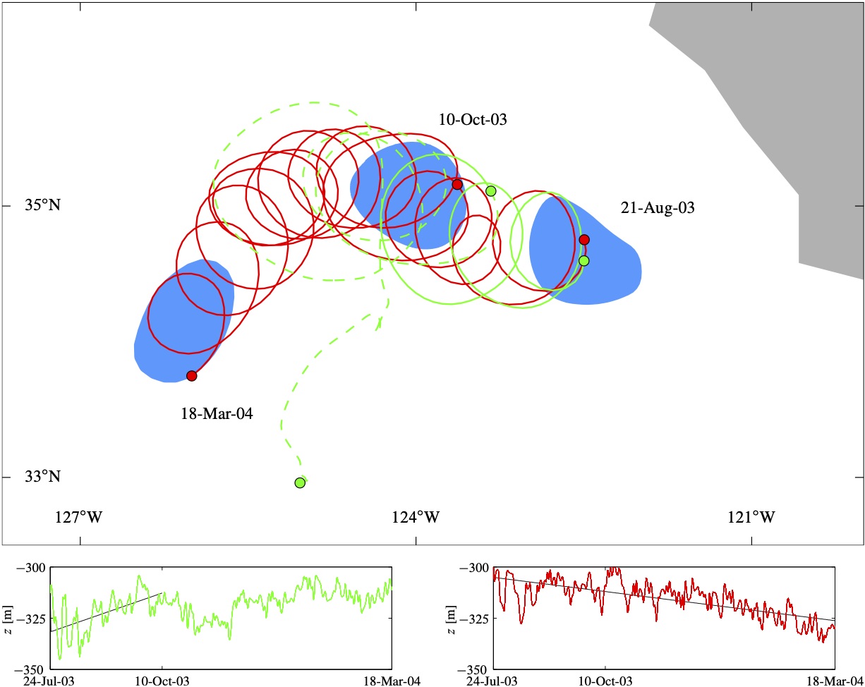
Figure 3: (top panel) Trajectories of two (acoustically tracked, submerged, quasi-isobaric) RAFOS floats (green and red) and snapshots of a California Undercurrent eddy or “cuddy,” detected from altimetry and classified as an RCE (light blue). The dots indicate the positions of the floats on the dates that this anticyclonic mesoscale eddy is shown. (bottom-left panel) As a function of time, depth of the green float and that of an equivalent light particle under the action of gravity, buoyancy, and Stokes drag over the period in which the float remains inside the eddy (black). (bottom-right panel) As in the right panel, but for the red float and a heavy particle. Adapted from Beron-Vera et al. (2015).

Initially close together, the two floats (indicated in red and green in the top panel of Fig. 3) were seen to take significantly divergent trajectories on roughly the same depth level (320 m). This behavior at first glance might be attributed to sensitive dependence of trajectories on initial positions in a turbulent ocean. But analysis of satellite altimetry measurements of sea-surface height Le Traon et al. (1998) reveals that the floats on the date of closest proximity fall within a California Undercurrent eddy or “cuddy” Garfield et al. (1999) which is furthermore classified as a coherent Lagrangian eddy Beron-Vera et al. (2015). (Sea-surface height, $\eta$, represents a flow streamfunction ($\psi$) under the assumption of a quasigeostrophic balance between the Coriolis force and the pressure gradient force, with the latter resulting exclusively from differences in $\eta$ (e.g., Beron-Vera et al., 2008).) However, while one float is seen to loop anticyclonically accompanying this mesoscale eddy very closely, the other float anticyclonically spirals away from the eddy rather quickly (the portion of the trajectory when the float is outside of the eddy is indicated in dashed).

The above seeming contradiction is resolved by noting that the green float experiences a net ascending motion from 24 July 2003, the beginning of the record, through about 10 October 2003, roughly when the float escapes the coherent Lagrangian eddy, detected from altimetry on 21 August 2003 (Fig. 3, bottom-left panel). By contrast, the red float indicated oscillates about a constant depth over this period, but experiences a net descending motion from 10 October 2003 until the end of the observational record, 18 March 2004 (Fig. 3, bottom-right panel). Positive overall buoyancy can thus be inferred for the green float from the beginning of the observational record until about 10 October 2003. By contrast, negative overall buoyancy, preceded by a short period of neutral overall buoyancy, can be inferred for the red float over the entire observational record.

The sign of the overall buoyancy of each float can be used to describe its behavior qualitatively using Thm. 3.1. The green float remains within the anticyclonic coherent Lagrangian eddy from 21 August to around 10 October 2003, nearly when it leaves the eddy and does not come back during the total observational record (about 6 months). This is qualitatively consistent with the behavior of a light particle. Beyond 10 October 2003, the buoyancy sign for this float is not relevant, given that it is already outside the eddy. In contrast, the red float remains inside the Lagrangian eddy over the whole observational record. This is qualitatively consistent with the behavior of a heavy particle.

The quantitative analysis in App. D of Beron-Vera et al. (2015) shows that $\delta-1\approx 0.5$ and $-0.1\times 10^{-10}$ for the green (light) and red (heavy) floats, respectively, both characterized by an inertial response time $\tau\approx 0.1$ d. Taking $V=0.1$ ms^-1 and $L=50$ km as upper bounds on the tangential speed and radius of cuddies (Steinberg et al., 2019), respectively, one gets $\smash{\frac{\tau}{L/V}}\approx 0.01$, which justifies modeling the floats as inertial particles.

Remark 15

Comparisons of theoretical predictions with additional observations are presented in Beron-Vera et al. (2015). These turned out to be relatively less successful than the comparison just described. The main reason is the inability of the geophysically adapted Maxey–Riley set to fully describe inertial ocean dynamics in the presence of windage, which is the subject hereafter.

4 Maxey–Riley equation for surface ocean inertial dynamics

The original Maxey–Riley equation and the geophysical adaptation discussed above assume that the particles are immersed in the fluid. This constrains the transferability of the latter to ocean as it cannot fully describe the motion of floating matter such as marine debris of varied kinds Trinanes et al. (2016); Miron et al. (2019). This is mainly due to its inability to simulate the effects of the combined action of ocean currents and wind drag. These effects were accounted for in a recent further adaptation of the Maxey–Riley equation to oceanography by Beron-Vera, Olascoaga and Miron Beron-Vera et al. (2019). The resulting equation, referred to as the BOM equation, was tested quite positively in the field Olascoaga et al. (2020); Miron et al. (2020b) as well as in the laboratory Miron et al. (2020a).

4.1 The BOM equation

Consider a stack of two homogeneous fluid layers separated by an interface fixed at $z=0$ ($z$ is the vertical coordinate), which rotates with angular speed $\frac{1}{2}f$, where $f(=f_{0}+\beta x^{2}$) is the Coriolis parameter (Fig. 4). The fluid in the bottom layer represents the seawater and has density $\rho$. The top-layer fluid is much lighter, representing the air; its density is $\rho_{\mathrm{a}}\ll\rho$. Let $\mu$ and $\mu_{\mathrm{a}}$ stand for dynamic viscosities of seawater and air, respectively. The seawater and air velocities vary in horizontal position and time, and are denoted $v(x,t)$ and $v_{\mathrm{a}}(x,t)$, respectively. Consider finally a solid spherical particle (of small radius $a$ and density $\rho_{\mathrm{p}}$) floating at the air–sea interface.

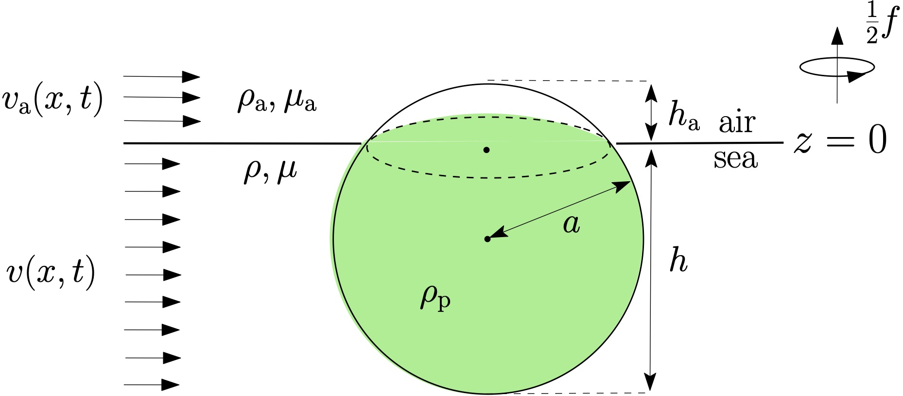
Figure 4: Solid spherical particle that floats at an assumed flat interface between homogeneous seawater and air, and is subjected to flow, added mass, and drag forces resulting from the action of unsteady, horizontally sheared ocean currents and winds. The various variables and parameters are defined in the text. Adapted from Beron-Vera et al. (2019).

The exact fraction of submerged particle volume Beron-Vera et al. (2019); Olascoaga et al. (2020)

$$\sigma=\frac{1-\delta_{\mathrm{a}}}{\delta-\delta_{\mathrm{a}}},$$ (51)

where

$$1\leq\delta\leq\frac{\rho}{\rho_{\mathrm{a}}}\gg 1,\quad\frac{\rho_{\mathrm{a}}}{\rho}\leq\delta_{\mathrm{a}}:=\frac{\rho_{\mathrm{a}}}{\rho_{\mathrm{p}}}\leq 1,$$ (52)

as static stability (Archimedes’ principle) demands, so $0\leq\sigma\leq 1$. The quantity $1-\sigma$ is sometimes referred to as reserved volume. Note that $\rho\gg\rho_{\mathrm{a}}$ implies $\delta\gg\delta_{\mathrm{a}}$ and as a result $\sigma\approx(1-\delta_{\mathrm{a}})/\delta$, which may be further approximated by $\delta^{-1}$ if $\delta_{\mathrm{a}}\ll 1$, which we will assume herein.

Remark 16

It is important to realize that $\sigma\approx\delta^{-1}$ does not follow from $\rho\ll\rho_{\mathrm{a}}$ as incorrectly stated in Beron-Vera et al. (2019). It is an assumption which holds provided that $\delta$ is not too large. This follows from noting that $\delta_{\mathrm{a}}\equiv(\rho_{\mathrm{a}}/\rho)\delta$. Thus inferences made in Beron-Vera et al. (2019) on behavior of the BOM equation, presented below, as $\delta\to\infty$ are not formally correct and should be ignored or interpreted with the these comments in mind Olascoaga et al. (2020).

Remark 17

The configuration in Fig. 4 is susceptible to (Kelvin–Helmholtz) instability Le Blond and Mysak (1978), which is ignored assuming that the air–sea interface remains horizontal at all times. In other words, any wave-induced Stokes drift Phillips (1997) is accounted for implicitly, and admittedly only partially, by absorbing its effects in the water velocity $v$ (e.g., as it would be directly measured or produced by some coupled ocean–wave–atmosphere model).

The emerged (resp., submerged) particle piece’s height $h_{\mathrm{a}}$ (resp., $h=2a-h_{\mathrm{a}}$) can be expressed in terms of $\delta$ noting that

$$h_{\mathrm{a}}/a=\Phi:=\smash{\frac{\mathrm{i}\sqrt{3}}{2}}(\varphi^{-1}-\varphi)-\frac{1}{2}(\varphi^{-1}+\varphi)+1$$ (53)

$\in[0,2)$ , where

$$\varphi^{3}:=\mathrm{i}\sqrt{1-(2\delta^{-1}-1)^{2}}+2\delta^{-1}-1.$$ (54)

The emerged (resp., submerged) particle’s projected (in the flow direction) area $A_{\mathrm{a}}$ (resp., $A=\pi a^{2}-A_{\mathrm{a}}$) is also a function of $\delta$ since

$$A_{\mathrm{a}}/\pi a^{2}=\Psi:=\pi^{-1}\cos^{-1}(1-\Phi)-\pi^{-1}(1-\Phi)\sqrt{1-(1-\Phi)^{2}}$$ (55)

$\in[0,1)$.

Noting that fluid variables and parameters take different values when pertaining to seawater or air, e.g.,

$$v_{\mathrm{f}}(x,z,t)=\begin{cases}v_{\mathrm{a}}(x,t)&\text{if }z\in(0,h_{\mathrm{a}}],\\ v(x,t)&\text{if }z\in[-h,0),\end{cases}$$ (56)

the BOM equation follows by vertically averaging each term of the original Maxey–Riley equation, adapted to account for Earth’s rotation effects, over the vertical extent $z\in[-h,h_{\mathrm{a}}]$ of the particle. The result is Beron-Vera et al. (2019)

$$\dot{v}_{\mathrm{p}}+\Big{(}\left(f+\tfrac{1}{3}R\omega\right)J+\frac{\operatorname{Id}}{\tau}\Big{)}v_{\mathrm{p}}=R\frac{\operatorname{D}\!{v}}{\operatorname{D}\!{t}}+R\left(f+\tfrac{1}{3}\omega\right)Jv+\frac{u}{\tau},$$ (57)

where

$$u:=(1-\alpha)v+\alpha v_{\mathrm{a}}$$ (58)

and $\smash{\frac{\operatorname{D}\!{}}{\operatorname{D}\!{t}}}v=\partial_{t}v+(\nabla v)v$ (for a full spherical version of (57), cf. App. A of Ref. Beron-Vera et al., 2019).

Primary BOM equation parameters $a$ and $\delta$ determine secondary parameters $\alpha$, $R$, and $\tau$ as follows:

$$\alpha:=\frac{\gamma\Psi}{1+(\gamma-1)\Psi}$$ (59)

$\in[0,1)$, which makes the convex combination (58) a weighted average of water and air velocities ($\gamma\approx 0.0167$ is the air-to-water viscosity ratio);

$$R:=\frac{1-\frac{1}{2}\Phi}{1-\frac{1}{6}\Phi}$$ (60)

$\in[0,1)$ and

$$\tau:=\frac{1-\frac{1}{6}\Phi}{\big{(}1+(\gamma-1)\Psi\big{)}\delta^{4}}\cdot\frac{a^{2}\rho}{3\mu}$$ (61)

$>0$, which measures the inertial response time of the medium to a particle floating at the air–sea interface.

Remark 18

Note that parameters $R$ and $\tau$ of the BOM equations are different than those involved in the original (and geophysically adapted) Maxey–Riley equation(s). The same symbols are used with no fear of confusion so the structure of the BOM equation resembles as closely as possible that of the original Maxey–Riley equation.

Remark 19

In writing (59) and (61) we followed the closure proposal made by Olascoaga et al. (2020) to fully determine parameters $R$ and $\tau$ in terms of the carrying fluid system properties and inertial particle characteristics. The original formulation Beron-Vera et al. (2019) of these parameters involved projected length factors, $k$ and $k_{\mathrm{a}}$. These should depend on how much the sphere is exposed to the air or immersed in the water to account for the effect of the air–sea interface (boundary) on the determination of the drag. The closure proposal in Olascoaga et al. (2020), $k=k_{\mathrm{a}}=\delta^{-3}$, assures the air component of the carrying flow field to dominate over the water component as the particle gets exposed to the air while reducing differences with observations. A stronger foundation for this closure should be sought, possibly resorting on direct numerical simulations of low-Reynolds-number flow around an spherical cap of different heights. To the best of our knowledge, a drag coefficient formula for this specific setup is lacking. An important aspect that these simulations should account for is the effect of the boundary on which the spherical cap rests on. Recent efforts in this direction are reported in (Zeugin et al., 2020).

Remark 20

The BOM equation was obtained assuming $\sigma\approx\delta^{-1}$. A more correct way to formulate the BOM equation so it is valid for all possible $\delta$ values is by using the exact form of $\sigma$, as given in (51). This way the $\sigma\to 0$ (equivalently, $\delta\to\infty$) limit is symmetric with respect to the $\sigma\to 1$ (equivalently, $\delta\to 1$) limit, as it can be expected. Also, additional terms, involving air quantities should be included, both in the full BOM equation and its reduced, slow-manifold approximation, presented below, if $\delta$ is allowed to take values in its full nominal range. However, since $\delta<10$ or so, typically, these additional terms can be safely neglected.

Remark 21

The weighted average of water and air velocities $u$ in (58) plays a very important role in short-term evolution (Olascoaga et al., 2020; Miron et al., 2020b), as we will review below. The velocity $u$ is of the type commonly discussed in the search-and-rescue literature and referred to as “leeway” velocity Breivik et al. (2013). An important difference between (58) and the leeway modeling approach is that (58) follows from vertically averaging the drag force rather as an ad-hoc proposition that involves an educated guess of leeway parameter $\alpha$ (e.g., Trinanes et al., 2016; Allshouse et al., 2017)) or informed by neglecting inertial effects and assuming an exact cancellation of water and air (quadratic) drags Röhrs et al. (2012); Nesterov (2018), which is at odds with the Maxey–Riley framework.

Remark 22

In deriving the BOM equation (57) it is assumed that the particle Reynolds number $\operatorname{Re_{p}}$ (10) is small both above and below the air–sea interface, which might thought difficult to be satisfied given the difference in water and air speeds. However, results from field (Olascoaga et al., 2020; Miron et al., 2020b) and laboratory (Miron et al., 2020a) experiments, reviewed below, justify the assumption of a Stokes regime in the water and the air. This provides support to the earlier suggestion (Beron-Vera et al., 2019) that an appropriate way to define $\operatorname{Re_{p}}$ is using $V_{\mathrm{slip}}=|v_{\mathrm{p}}-u|$, which is $O(\varepsilon)$ for sufficiently small particles, fulfilling the small $\operatorname{Re_{p}}$ requirement.

4.2 Slow-manifold approximation

Assume that both $v(x,t)$ and $v_{\mathrm{a}}(x,t)$ are smooth in each of their arguments. In the limit when $\tau=O(\varepsilon)$ as $\varepsilon\to 0$, the BOM equation (57) involves both slow ($x$) and fast ($v_{\mathrm{p}}$) variables, which makes it a singular perturbation problem, just as the Maxey–Riley equation (7) and its geophysical adaptation (41) under a similar assumption. In these circumstances one can apply nonautonomous GSPT to obtain the following reduced equation Beron-Vera et al. (2019):

$$\dot{x}=v_{\mathrm{p}}=u+u_{\tau}$$ (62)

$+\,O(\varepsilon^{2})$, where

$$u_{\tau}:=\tau\left(R\frac{\operatorname{D}\!{v}}{\operatorname{D}\!{t}}+R\Big{(}f+\frac{1}{3}\omega\Big{)}Jv-\frac{\operatorname{D}\!{u}}{\operatorname{D}\!{t}}-\Big{(}f+\frac{1}{3}R\omega\Big{)}Ju\right)$$ (63)

with $\smash{\frac{\operatorname{D}\!{}}{\operatorname{D}\!{t}}}u=\partial_{t}u+(\nabla u)u$, i.e., the total derivative of $u$ along a trajectory of $u$.

The reduced equation (62) controls the evolution of the full equation (57) on the slow manifold, defined by

$$M_{\tau}:=\big{\{}(x,v_{\mathrm{p}},t):v_{\mathrm{p}}=u(x,t)+u_{\tau}(x,t)\big{\}}.$$ (64)

Being $C^{r}O(\varepsilon)$-close to the critical manifold, given by

$$M_{0}:=\big{\{}(x,v_{\mathrm{p}},t):v_{\mathrm{p}}=u(x,t)\big{\}},$$ (65)

for any $r<\infty$, and unique up to an error much smaller than $O(\varepsilon)$, $M_{\tau}$ is a locally invariant, normally hyperbolic manifold that attracts all solutions of (57) exponentially fast. The only caveat Haller and Sapsis (2008) is that rapid changes in the carrying flow velocity, represented by $u$, can turn the exponentially dominated convergence of solutions on $M_{\tau}$ not necessarily monotonic over finite time.

Remark 23

The carrying flow ($u$) that defines the critical manifold $M_{0}$ depends on the buoyancy of the particle and thus has inertial effects built in. Inertial effects are felt by the particle even during the initial stages of the evolution, which are controlled by $\dot{x}=u$ provided that $v_{p}$ initially at $t=t_{0}$ is $O(\varepsilon)$-close to $u$, as it follows from the smooth dependence of the solutions of (57) on parameters. This is important in comparisons with field and laboratory observations, which we discuss below after illustrating long-time asymptotic aspects of the BOM equation.

Remark 24

For neutrally buoyant particles ($\delta=1$) the BOM equation reduces exactly to (25) except that $A=-\smash{\big{(}}\nabla v+(f+\smash{\tfrac{1}{3}}\omega)J+\tau^{-1}\operatorname{Id}\smash{\big{)}}$. However, all the results stated in Sec. 2.4 relating to the stability of the neutral manifold $N$ (24) hold Beron-Vera et al. (2019). An important observation is that, unlike in the original Maxey–Riley equation (7) and its geophysical adaptation (41), $N$ does not coincide with the critical manifold $M_{0}$ (65).

4.3 Local instability of the slow manifold

Applying the local instability analysis of Haller and Sapsis (2010), discussed in Remark 34, on the slow manifold of the BOM equation (64), one finds that perturbations off it will grow where

$$\tau>\frac{2}{\sqrt{(\partial_{1}u^{1}-\partial_{2}u^{2})^{2}+(\partial_{2}u^{1}+\partial_{1}u^{2})^{2}}-\nabla\cdot u}.$$ (66)

This new result follows upon noting that $\Gamma=-\smash{\big{(}}\nabla u+(f+\smash{\tfrac{1}{3}}R\omega)J+\tau^{-1}\operatorname{Id}\smash{\big{)}}+O(\varepsilon)$, which leads to $\Gamma+\Gamma^{\top}=-\nabla u-(\nabla u)^{\top}-2\tau^{-1}\operatorname{Id}+O(\varepsilon)$. Note that neither the lift term nor the Coriolis force contribute to set the instability of the slow manifold, a property of the Maxey–Riley equation (7) and its geophysical adaptation (41). The practical consequence of the result just presented awaits to be investigated.

4.4 Behavior near quasigeostrophic eddies

Theorem 3.1, though successful in describing the behavior of submerged floats, falls short at explaining an observed Brach et al. (2018) tendency of floating plastic debris to collect inside anticyclonic mesoscale eddies while avoiding cyclonic ones. The BOM equation turns out to be capable of describing this observation, as articulated next.

Oceanic mesoscale eddies (with diameters ranging from 50 to 250 km) are characterized by a low Rossby number Pedlosky (1987), so it is reasonable to explore the local stability of floating inertial particles near the center of quasigeostrophic RCE as done to arrive at Thm. 3.1. The starting point is the reduced BOM equation (62), approximated by

$$\dot{x}=v_{\mathrm{p}}=gf_{0}^{-1}J\nabla\eta+\tau g(1-\alpha-R)\nabla\eta$$ (67)

$+\,O(\varepsilon^{2})$. This approximations holds under the following assumptions. First, $v=gf_{0}^{-1}J\nabla\eta+O(\varepsilon^{2})$, where $\eta(x,t)$ is sea surface height and $g$ stands for gravity, $\partial_{t}=O(\varepsilon)$, and $f=f_{0}+O(\varepsilon)$. Second $\alpha=O(\varepsilon)$, at least, consistent with it being very small (a few percent) over a large range of buoyancy ($\delta$) values. Third, $v_{\mathrm{a}}=O(\varepsilon^{2})$, at least, i.e., the wind field over the period of interest is sufficiently weak (calm).

Applying on (67) the same local stability analysis that led to Thm. 3.1, one finds Beron-Vera et al. (2019)

$$\det\operatorname{D}\!{\mathbf{F}_{t_{0}}^{t_{0}+T}(x_{0}^{*})}=\exp\tau\big{(}1-R-\alpha\big{)}f_{0}\,\mathrm{sLAVD}_{t_{0}}^{t_{0}+T}(x_{0}^{*})$$ (68)

$+\,O(\varepsilon^{2})$ where

$$\mathrm{sLAVD}_{t_{0}}^{t_{0}+T}(x_{0}^{*}):=\!\!\!\operatorname*{sign}_{t\in[t_{0},t_{0}+T]}\!\!\!gf_{0}^{-1}\nabla^{2}\psi(F_{t_{0}}^{t}(x_{0}^{*}),t),t)\,\mathrm{LAVD}_{t_{0}}^{t_{0}+T}(x_{0}^{*}).$$ (69)

Since $1-R\geq\alpha\geq 0$, on can state the following:

Theorem 4.1 (Beron-Vera, Miron and Olascoaga Beron-Vera et al. (2019))

The trajectory of the center of an anticyclonic ($f_{0}\,\mathrm{sLAVD}<0$) RCE is a finite-time attractor for floating inertial particles, while that of a cyclonic ($f_{0}\,\mathrm{sLAVD}>0$) RCE is a finite-time repellor for floating inertial particles.

4.5 Great garbage patches

The ocean’s subtropical gyres are well-documented Cozar et al. (2014); Lebreton et al. (2018) to show a tendency to accumulate plastic debris forming large patches, particularly that of the North Pacific, known as the “Great Pacific Garbage Patch.” This tendency of floating matter to concentrate in the subtropical gyres has been noted Beron-Vera et al. (2016) in the distribution of undrogued surface drifting buoys from the NOAA Global Drifter Program Lumpkin and Pazos (2007). A standard drifter from this program, which collects data since 1979, follows the Surface Velocity Program or SVP Niiler et al. (1987) design with a 15-m-long holey-sock drogue attached to it to minimize wind slippage and wave-induced drift, thereby maximizing its water tracking characteristics. However, the drogue is often lost after some time from deployment Lumpkin et al. (2012) while the satellite tracker included in the spherical float keeps transmitting positions.

The left panel of Fig. 5 shows positions at deployment time (light blue) and positions after a period of at least 1 yr (blue) of all SVP drifters that remained drogued over the entire period. The right panel shows positions where the drifters have lost their drogues (light blue) and positions taken by these drifters after at least 1 yr from those instances (blue). The initial positions are similarly homogeneously distributed. But there is a marked difference in the final positions: while the drogued drifters take a more homogeneous distribution, the undrogued drifters reveal a tendency to accumulate in the subtropical gyres.

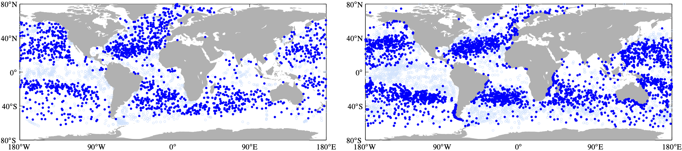
Figure 5: Initial (light blue) and final (blue) positions of drogued (left) and undrogued (right) SVP drifters from the NOAA Global Drifter Program over 1979–present. “Final position” refers to the last recorded position after at least 1 yr past the time at the “initial position,” which is the deployment position for drogued drifters or the location where a drifter loses the drogue.

The BOM equation is able to predict great garbage patches in the long run consistent with observed behavior, thereby allowing to interpret this behavior as produced by inertial effects. To see this one can consider Stommel’s Stommel (1948) conceptual model of wind-driven circulation as in Beron-Vera et al. (2019). The steady flow in such a barotropic (constant density) model is quasigeostrophic, i.e., $v=J\nabla\psi+O(\varepsilon^{2})$, and has an anticyclonic basin-wide gyre in the northern hemisphere, so $\omega=\nabla^{2}\psi\leq 0$, driven by steady westerlies and trade winds, $v_{\mathrm{a}}=W(x^{2})e_{1}$ with $W^{\prime}(x^{2})\geq 0$. The inertial particle velocity on the slow manifold (62) takes the form

$$v_{\mathrm{p}}=(1-\alpha)J\nabla\psi+\alpha We_{1}+\tau f_{0}\big{(}(1-R-\alpha)\nabla\psi-\alpha We_{2}\big{)}$$ (70)

with an $O(\varepsilon^{2})$ error. The divergence of this velocity is given by

$$\nabla\cdot v_{\mathrm{p}}=\tau f_{0}\big{(}(1-R-\alpha)\nabla^{2}\psi-\alpha W^{\prime}(x^{2})\big{)}.$$ (71)

Recalling that $1-R-\alpha\geq 0$, it follows that $\nabla\cdot v_{\mathrm{p}}\leq 0$, which promotes clustering of inertial particles in the interior of the gyre in a manner akin to undrogued drifters and plastic debris. Moreover, in Beron-Vera et al. (2019) it is shown that $\dot{x}=v_{\mathrm{p}}$, with $v_{\mathrm{p}}$ as in (70) with $\psi$ as given in Haidvogel and Bryan (1992) and $W$ deduced from the wind stress using a bulk formula, has a stable spiral equilibrium at $(x^{1},x^{2})=(\smash{\frac{r}{\beta}}\log\smash{\frac{\beta L}{r}},\smash{\frac{1}{2}}L)$ where $L$ is the side of an assumed square midlatitude domain and $r$ is the bottom friction coefficient. The right panel of Fig. 6 shows streamlines of $v_{\mathrm{p}}$ assuming $a=17.5$ cm and $\delta=2$ (which give $\alpha\approx 0.01$, $R\approx 0.6$, and $\tau\approx 0.01$ d, roughly characterizing undrogued drifters). Additional parameter choices, $H=200$ m (thermocline depth), $L=10$ Mm, $r=10^{-5}$ s^-1, $F=2\times 10^{-3}$ m²s^-2 (wind stress amplitude per unit density), and $C_{\mathrm{D}}=1.2\times 10^{-3}$ (drag coefficient). Note that a “leeway” model, i.e., one of the form $\dot{x}=u$, produces closed streamlines (Fig. 6, middle panel) just as the Stommel model streamlines (Fig. 6, left panel).

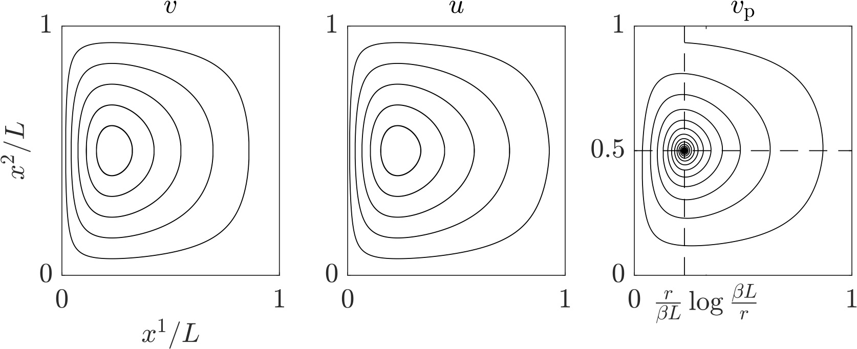
Figure 6: Streamlines of the Stommel wind-driven circulation model velocity (left), the $\delta$-weighted-average of this velocity and the wind field that drives the Stommel gyre (middle), and the inertial particle velocity on the slow manifold of the BOM equation resulting from using these water and air velocities (right). Adapted from Beron-Vera et al. (2019).

Earlier studies have argued that the formation of great garbage patches in the subtropical gyres is due to wind-induced downwelling in such regions. This is not represented in Stommel’s model for being a higher order (in the Rossby number) effect. Beron-Vera, Olascoaga and Lumpkin Beron-Vera et al. (2016) showed that clustering of undrogued drifters in the subtropical gyres (Fig. 7), which is visible already after about 1.5 yr, is too fast to be explained by wind-induced downwelling. This was done by comparing the long-term evolution of trajectories of $\dot{x}=v$, with $v$ produced by a general ocean circulation model, with that of floating inertial particles evolving under an earlier form of the BOM equation. Such an earlier form the BOM equation was obtained by modeling the submerged (resp., emerged) particle portion as a sphere of the fractional volume that is submerged (resp., emerged) while it evolves under the geophysically adapted Maxey–Riley equation. Despite this earlier form of the BOM equation was successful in explaining great garbage patch formation, it could not explain the observed tendency of anticyclonic eddies to trap plastic debris, which motivated the derivation of its successor.

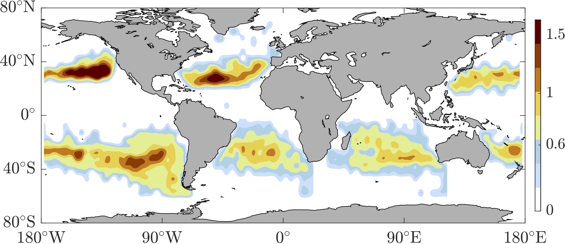
Figure 7: Expressed as number per degree squared, density of inertial particles after 1.5 yr normalized by density in the initially uniform distribution of particles over the global surface ocean. The water velocity is given by surface ocean velocity output from the Hybrid-Coordinate Ocean Model. The air velocity corresponds to the wind velocity from the reanalysis used to construct the wind stress that forces the model. Adapted from Beron-Vera et al. (2016).

4.6 Field experiments verification

Olascoaga et al. Olascoaga et al. (2020) present results from a field experiment that provides support to the BOM equation. The field experiment consisted in deploying simultaneously specially designed drifters of varied sizes, buoyancies, and shapes off the southeastern Florida Peninsula in the Florida Current, and subsequently tracking them via satellite. Four types of special drifters were involved in the experiment, mimicking debris found in the ocean. The main bodies of these special drifters represented a sphere of radius 12 cm, approximately, a cube of about 25 cm side, and a cuboid of approximate dimensions 30 cm $\times$ 30 cm $\times$ 10 cm. These special drifters were submerged below the sea level by roughly 10, 6.5, and 5 cm, respectively. The fourth special drifter consisted in an artificial boxwood hedge of about 250 cm $\times$ 50 cm and thickness of nearly 2 cm. It floated on the surface with the majority of its body slightly above the surface.

To account for the effects produced by the lack of sphericity of the special drifters, a simple heuristic fix, expected to be valid for sufficiently small objects, was used consisting in multiplying $\tau$ in (61) by $K$, a shape factor satisfying Ganser (1993)

$$K=\frac{3a_{\mathrm{v}}}{a_{\mathrm{n}}+2a_{\mathrm{s}}}.$$ (72)

Here $a_{\mathrm{n}}$, $a_{\mathrm{s}}$, and $a_{\mathrm{v}}$ are the radii of the sphere with equivalent projected area, surface area, and equivalent volume, respectively, whose average provide an appropriate choice for $a$.

		Parameter
		Primary				Secondary
Drifter type		$a$ [cm]	$K$	$\delta$		$\alpha$	$R$	$\tau$ [d]
Sphere		12	1.00	2.7		0.027	0.51	0.002
Cube		16	0.96	4.0		0.042	0.42	0.001
Cuboid		13	0.95	2.5		0.024	0.53	0.003
Hedge		26	0.53	1.3		0.005	0.79	0.031

Table 1: Parameters that characterize the special drifters as inertial particles.

The various parameters that characterize the special drifters as inertial “particles” are shown in Table 1. An a-priori dimensional analysis justifies treating them as such and thus using the BOM equation to investigate their motion. Let $V$ and $L$ be typical carrying fluid system velocity and length scales, respectively. Taking $V=1$ m s^-1, typical at the axis of the Florida Current, and $L=50$ km, a rough measure of the width of the current, one obtains that $\smash{\frac{\tau}{L/V}}\ll 1$ for the special drifters as required since $L/V$ is of the order of 1 d and $\tau$ is much shorter than that for the drifters.

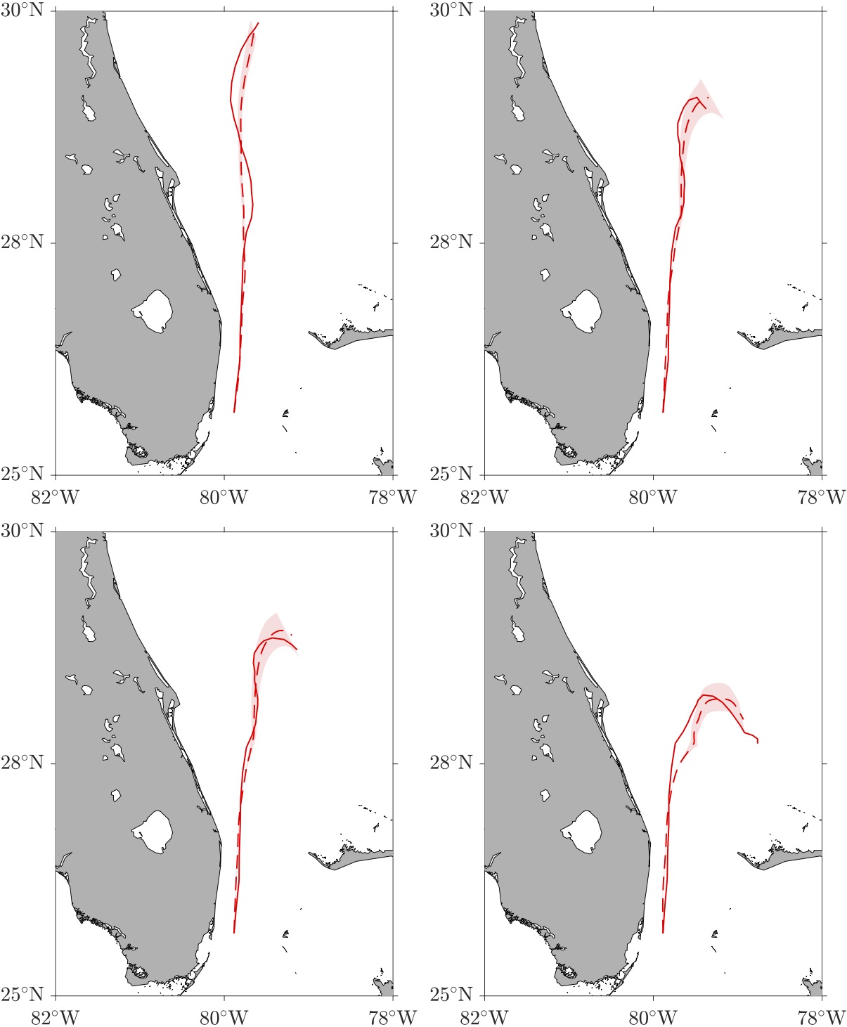
Figure 8: One-week-long trajectories of specially designed undrogued drifters with buoyancy increasing rightward (solid) along with trajectories produced by BOM equation (dashed; shades reflect uncertainty around drifter buoyancy determination). Adapted from Olascoaga et al. (2020).

Figure 8 shows week-long trajectories taken by the special drifters (solid curves) along with trajectories produced by the BOM equation (dashed curves with shades of red around reflecting an assumed 10%  uncertainty in the determination of the buoyancy of the drifters). The driving ocean currents are provided by an altimetry/wind/drifter data synthesis Olascoaga et al. (2020) and the winds are from reanalysis Dee et al. (2011). The special drifter trajectories were subjected to a strong wind event 2 to 3 days after deployment, which affected them differently mainly according to their buoyancy as described by the BOM equation. We note that $\tau$ turned out to be sufficiently small for the trajectories of the BOM equation (57), initialized from the special drifter deployment locations and velocities estimated by differentiating the special drifter trajectories, to be well approximated by those of $\dot{x}=u$ over the initial stages of the evolution.

Remark 25

Indeed, let $x(t;x_{0},t_{0})$ denote the trajectory of a particle starting from $x_{0}$ at time $t_{0}$. By smooth dependence of the solutions of the BOM equation (57) on parameters, if the particle is initialized with velocity $u(x_{0},t_{0})$, then $v_{\mathrm{p}}$ will remain $O(\varepsilon)$-close to $u(x(t;x_{0},t_{0}),t)$ over $[t_{0},t]$ finite. In other words, over finite $[t_{0},t]$ the trajectory of the particle will be mainly controlled by the integrated effect of the ocean current and wind drag, explaining why BOM equation trajectories in Fig. 8 were well approximated by those of $\dot{x}=u$.

Remark 26

Further support for the validity of the BOM equation is provided by Miron et al. Miron et al. (2020b), who considered a much larger set of longer special drifter trajectories, starting from several locations in the tropical North Atlantic. Since various special drifters of the same type were included in each deployment, a cluster analysis was possible to be carried out showing grouping of trajectories depending on drifter design. This added further support to the importance of inertial effects on floating matter drift. Special drifter trajectories and BOM equation trajectories in many cases showed very good agreement. As in Olascoaga et al. (2020) the latter were seen to be well approximated by those of $\dot{x}=u$ despite their longer extent (one month or longer vs. one week). Disagreements were mainly attributed to limitations of the carrying flow system representation as assessed by the low skill of the ocean current representation in describing the motion of drogued drifters, also included in the experiments.

4.7 Laboratory verification

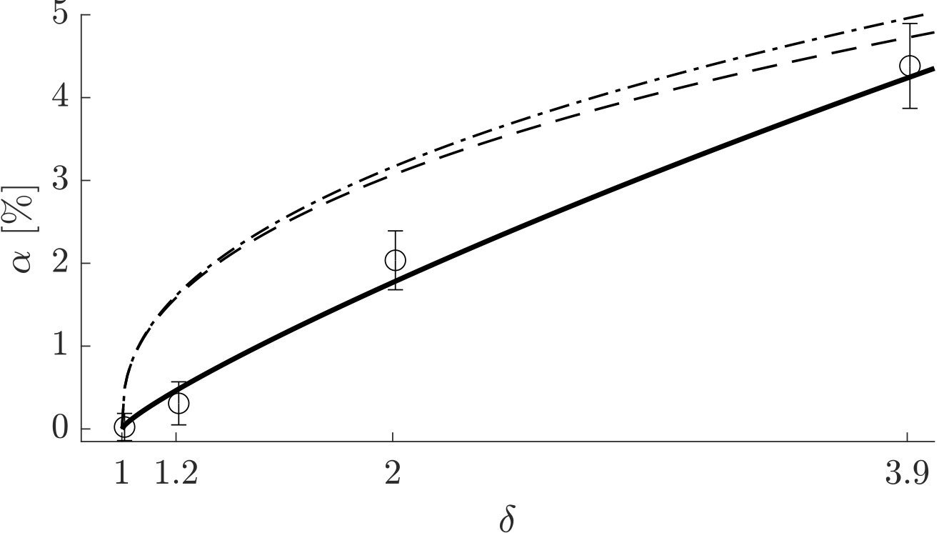
Figure 9: As a function of buoyancy, estimated (circles) and theoretical (solid curve) “leeway” factor. The accompanying error bar represent one standard deviation uncertainties. The dashed and dot-dashed curves are buoyancy-dependent “leeway” models derived in (Nesterov, 2018) and (Röhrs et al., 2012), respectively. Adapted from Miron et al. (2020a).

Miron et al. Miron et al. (2020a) report results from a series of experiments in an air–water stream flume facility that provide controlled observational support for the buoyancy dependence of the BOM equation’s carrying flow velocity. This was found to play a very important role in the field experiments just described, despite the rough estimates of the buoyancy of the drifters in the tropical North Atlantic experiments and the admittedly poor representations of the carrying ocean currents and winds were available, both in the Florida Current and tropical North Atlantic experiments.

The laboratory experiments were designed to specifically validate the dependence of the “leeway” factor $\alpha$ on $\delta$ in (59). This was done by noting that when $v$ and $v_{\mathrm{a}}$ are constant, and hence $u$ as well, in the nonrotating case,

$$v_{\mathrm{p}}(t)=v_{\mathrm{p}}(0)\mathrm{e}^{-t/\tau}+(1-\alpha)v+\alpha v_{\mathrm{a}}$$ (73)

exactly solves the BOM equation (57), which allows us to estimate $\alpha$ as a function of $\delta$ given $v$ and $v_{\mathrm{a}}$ and measurements of $v_{\mathrm{p}}$ in the along-flume direction.

The laboratory experiments were carried out Medina (2020) in the Air-Sea Interaction Salt-water Tank (ASIST) of the Alfred G. Glassell, Jr. SUrge STructure Atmosphere INteraction (SUSTAIN) facility of the University of Miami’s Rosenstiel School of Marine & Atmospheric Science (https://sustain.rsmas.miami.edu/). ASIST offers the possibility to control the water stream with a pump and the air stream using a fan.

Four thick rubber, deformation resistant balloons of equal radius $a=0.11$ m were employed in the experiments. These were filled with different water levels so that $\delta\approx$ 3.9, 2, 1.2, and 1, which represent a fairly range of $\delta$ values given that the corresponding submerged-depth-to-diameter ratios are $h/2a\approx 0.33$, 0.5, 0.75, and 1.

The circles in Fig. 9 are mean (over several experiment realizations) $\alpha$ values estimated from (73) taking $v$ as the vertical average of the water stream profile (estimated using particle image velocimetry Novelli et al. (2017)) over a balloon diameter (the balloon velocities were estimated from video tracking). Error bars represent one standard deviation uncertainties. Note the very good agreement with the theoretical $\alpha(\delta)$ curve (59), shown as solid curve. Indeed, the agreement between measurements and the BOM equation prediction is much better than that between measurements and two buoyancy-dependent “leeway” parameter models discussed in the search-and-rescue literature Röhrs et al. (2012); Nesterov (2018), included for reference as dashed and dot-dashed curves, respectively.

Remark 27

The laboratory experiment results suggest that neglecting the Basset–Boussinesq history or memory term is indeed well justified despite being of the same order as the drag term. How this result is altered by flow unsteadiness is not known and should be investigated.

5 Maxey–Riley equation for elastically coupled floating particles

One additional extension of the Maxey–Riley equation is presented by Beron-Vera and Miron Beron-Vera and Miron (2020). This is motivated by an interest to understand the mechanism that leads Sargassum (a type of large brown seaweed) to inundate coastal waters and land on beaches, particularly those of the Caribbean Sea. This phenomenon has been on the rise since 2011 Wang et al. (2019); Johns et al. (2020) and is challenging scientists, coastal resource managers, and administrators at local and regional levels Langin (2018).

5.1 The Sargassum drift model

A raft of pelagic Sargassum is composed of flexible stems which are kept afloat by means of bladders filled with gas while it drifts under the action of ocean currents and winds. Beron-Vera and Miron Beron-Vera and Miron (2020) proposed a mathematical model for this physical depiction of a drifting Sargassum raft as an elastic network of buoyant, finite-size particles that evolve according to the BOM equation.

To construct the mathematical model, Beron-Vera and Miron Beron-Vera and Miron (2020) consider a network of $N>1$ spherical particles (beads) connected by (massless, nonbendable) springs. The (small) particles are assumed to have $\delta\geq 1$ finite. The elastic force (per unit mass) exerted on particle $i$, with two-dimensional Cartesian position $x_{i}=(x^{1}_{i},x^{2}_{i})$, by neighboring particles at positions $\{x_{j}:j\in\operatorname{neighbor}(i)\}$, is assumed to obey Hooke’s law (e.g., Goldstein (1981)):

$$F_{i}=-\sum_{j\in\operatorname{neighbor}(i)}k_{ij}\big{(}|x_{ij}|-\ell_{ij}\big{)}\frac{x_{ij}}{|x_{ij}|},$$ (74)

$i=1,\dotsc,N$, where

$$x_{ij}:=x_{i}-x_{j};$$ (75)

$k_{ij}\geq 0$ is the stiffness (per unit mass) of the spring connecting particle $i$ with neighboring particle $j$; and $\ell_{ij}\geq 0$ is the length of the latter at rest.

The Sargassum drift model is obtained by adding the elastic force (74) to the right-hand-side of the BOM equation. The result is a set of $N$ 2nd-order ordinary differential equations, coupled by the elastic term, viz.,

$$\dot{v}_{i}+\left(\left.f\right|_{i}+\tfrac{1}{3}R\left.\omega\right|_{i}\right)v_{i}^{\perp}+\frac{v_{i}}{\tau}=R\frac{\operatorname{D}\!{\left.v\right|_{i}}}{\operatorname{D}\!{t}}+R\left(\left.f\right|_{i}+\tfrac{1}{3}\left.\omega\right|_{i}\right)\left.v\right|_{i}^{\perp}+\frac{\left.u\right|_{i}}{\tau}+F_{i},$$ (76)

$i=1,\dotsc,N$, where $v_{i}$ is the velocity of particle $i$ and $\left.\right|_{i}$ means pertaining to particle $i$.

Because the elastic force (74) does not depend on velocity, the nonautonomous GSPT analysis of the BOM equation with $\tau=O(\varepsilon)$ as $\varepsilon\to 0$ Beron-Vera et al. (2019) applies to (76) with the only difference that the equations on the slow manifold are coupled by the elastic force (74), namely,

$$\dot{x}_{i}=v_{i}=\left.u\right|_{i}+\left.u_{\tau}\right|_{i}+\tau F_{i}+O(\tau^{2}),$$ (77)

$i=1,\dotsc,N$. The slow manifold of (76) is the $(2N+1)$-dimensional subset $\{(x_{i},v_{i},t):v_{i}=u(x_{i},t)+u_{\tau}(x_{i},t)+\tau F_{i}(x_{i};x_{j}:j\in\operatorname{neighbor}(i))+O(\tau^{2}),\,i=1,\dotsc,N\}$ of the $(4N+1)$-dimensional phase space $(x_{i},v_{i},t)$, $i=1,\dotsc,N$.

5.2 Behavior near quasigesotrophic eddies

Equation (77), which attracts all solutions of (76), can be approximated by

$$\dot{x}_{i}=v_{i}=gf_{0}^{-1}\nabla^{\perp}\left.\eta\right|_{i}+\tau\big{(}g(1-\alpha-R)\nabla\left.\eta\right|_{i}+F_{i}\big{)}$$ (78)

$+\,O(\varepsilon^{2})$, $i=1,\dotsc,N$, under the following assumptions. First, the near surface ocean flow is in quasigeostrophic balance, i.e., $v=gf_{0}^{-1}\nabla^{\perp}\eta+O(\varepsilon^{2})$, $\partial_{t}=O(\varepsilon)$, and $f=f_{0}+O(\varepsilon)$. Second, the elastic interaction does not alter the nature of the critical and slow manifolds, which is guaranteed by making $F_{i}=O(\varepsilon)$. Third, $\alpha=O(\varepsilon)$, at least, consistent with it being very small (a few percent) over a large range of buoyancy ($\delta$) values. Fourth, $v_{\mathrm{a}}=O(\varepsilon^{2})$, at least, i.e., the wind field over the period of interest is sufficiently weak (calm).

Applying a local stability analysis similar to the one applied on (43) and (67), one obtains the following:

Theorem 5.1 (Beron-Vera and Miron Beron-Vera and Miron (2020))

The trajectory of the center of an RCE, $F_{t_{0}}^{t}(x_{0}^{*})$, is locally forward attracting overall over $t\in[t_{0},t_{0}+T]$:

1. for all $k_{ij}$ when $\operatorname*{sign}_{t\in[t_{0},t_{0}+T]}\nabla^{2}\eta(F_{t_{0}}^{t}(x_{0}^{*}),t)<0$; and

2. provided that

   $$|T|\sum_{i=1}^{N}\sum_{j\in\operatorname{neighbor}(i)}k_{ij}>gN(1-\alpha-R)\left|\int_{t_{0}}^{t_{0}+T}|\nabla^{2}\eta(F_{t_{0}}^{t}(x_{0}^{*}),t)|\operatorname{d}\!{t}\right|$$ (79)

   when $\operatorname*{sign}_{t\in[t_{0},t_{0}+T]}\nabla^{2}\eta(F_{t_{0}}^{t}(x_{0}^{*}),t)>0$.

Since $\omega=gf_{0}^{-1}\nabla^{2}\eta+O(\varepsilon^{2})$, the above result says that the center of a cyclonic rotationally coherent quasigeostrophic eddy represents a finite-time attractor for elastic networks of inertial particles in the presence of calm winds if they are sufficiently stiff, while that of an anticyclonic eddy irrespective of how stiff.

Table

Type of inertial particle(s)	Cyclonic vortices	Anticyclonic vortices	Thm.
Submerged, light	Attract	Repel	1
Submerged, heavy	Repel	Attract	1
Floating, free	Repel	Attract	2
Floating, elastic network, weakly stiff	Repel	Attract	3
Floating, elastic network, strongly stiff	Attract	Attract	3

Table 2: Summary of the results from Thms. 3.1–5.1.

5.3 Reality check

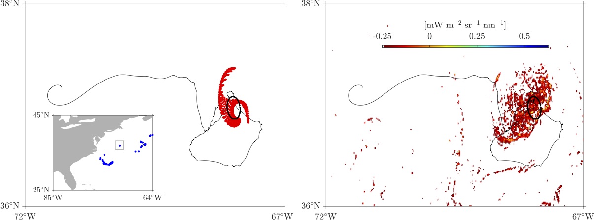
Figure 10: (left panel) Elastically interacting inertial particles (red) concentrating inside a cold-core (i.e., cyclonic) Gulf Stream ring (with boundary depicted in thick black and trajectory indicated by the thin black curve) compared to noninteracting particles that are repelled away from the ring (blue). The ring was inferred from altimetry and classified as an RCE. The particles, whose positions are shown on 7 October 2006, were initiated 6 months earlier from exactly the same locations near the boundary of the ring. (right panel) The boundary of the ring on the left with observed Sargassum concentrating within (Sargassum corresponds to Maximum Chlorophyll Index (MCI) values exceeding $-0.25$ mW m^-2sr^-1nm^-1).

The predictions of Thm. 5.1 are consistent with observations, as is exemplified in Fig. 10. Blue dots in the left panel are noninteracting inertial particles, while red dots are inertial particles connected elastically. The particles, whose positions are shown on 7 October 2006, were initiated 6 months earlier from exactly the same locations near the boundary of a cold-core (i.e., cyclonic) Gulf Stream ring. Detected from altimetry and classified as an RCE, the boundary of the ring is depicted in thick black. Its trajectory (since 10 April 2006) is indicated by the thin black curve. In the simulation, the network’s springs are taken of equal length at rest, $\ell_{ij}=0.5$ m. The beads, totalling $n=625$, have a common radius $a=0.1$ m. The buoyancies of the beads are all taken the same and equal to $\delta=1.25$, following Olascoaga et al. Olascoaga et al. (2020). The resulting inertial parameters $\alpha=5.9\times 10^{-3}$, $R=0.6$, and $\tau=4.1\times 1^{-2}$.

Note the effect of the ring on the elastically interacting particles. This is in stark contrast with that on the noninteracting inertial particles, which are repelled way away from the ring. Indeed, on 7 October 2006 the noninteracting particles lie more than 1000 km away from the ring. The concentration of the elastically interacting particles inside the cyclonic RCE, predicted by Thm. 5.1.2, is consistent with the observation, shown in the right panel of Fig. 10, of Sargassum as inferred from MODIS (Moderate Resolution Imaging Spectroradiometer) satellite imagery. Note that the concentration of Sargassum is high in the Gulf Stream ring in question.

Remark 28

An important observation is that the elastically interacting particles have been evolved under the full system (76) rather than (78), which approximates the reduced system (77) assuming quasigeostrophic ocean currents and calm wind conditions. While the ocean currents were inferred from altimetry, which is consistent with the quasigeostrophic assumption, the wind was provided by reanalysis data with no restriction of any kind on its intensity. This suggests that Thm. 5.1 is valid on a wider range of conditions than formally required.

Remark 29

The oceanographic relevance of the results above is that eddies, observed to propagate westward Morrow et al. (2004) consistent with theoretical expectation Cushman-Roisin et al. (1990), can provide an effective mechanism for the connectivity of Sargassum between the Intra-Americas Sea and remote regions in the tropical/equatorial Atlantic.

6 Concluding remarks

Despite the significant progress already made in recent years to port the Maxey–Riley framework to oceanography, a number of aspects still need to be accounted for to expand its applicability. For instance, at present wave-induced drift effects are represented implicitly in the BOM equation, at the carrying flow system level. Explicit representation of these effects, whose importance awaits to be carefully assessed, should account for the tendency of waves to push objects downward when they are close to the air–sea interface, which might be parametrized by making the object’s buoyancy a function of the angle of wave attack. This would require controlled experimentation in a wind-wave tank facility. Shape effects are at the moment represented heuristically. Direct computational fluid dynamics experimentation would be needed to derive appropriate formulas for the drag depending on the object’s shape. Sinking and rising of plastic debris as well as Sargassum rafts are reported. This would require one to include a buoyancy force. Clearly, in this case a reliable representation of three-dimensional ocean currents would be critical. Physiological changes of Sargassum are necessary to be accounted to enable a more accurate description of the evolution of rafts. This should minimally control the growth and decay of size of the elastic networks as they drift across regions of the ocean with varying thermal and geochemical conditions. The practical utility of the BOM equation is not restricted to marine debris and Sargassum raft motion prediction. Among the many additional problems that the BOM equation should be useful for are search-and-rescue operations at sea and the drift of sea-ice in a warming climate. In every case the nonlinear dynamics techniques and results overviewed here once appropriately adapted are expected to facilitate the understanding of observed behavior as well as predicting behavior yet to be observed.

Conflict of interest

The author declares that he has no conflict of interest.

References

- Aksamit et al. (2020) Aksamit N, Sapsis T, Haller G (2020) Machine-learning mesoscale and submesoscale surface dynamics from Lagrangian ocean drifter trajectories. J Phys Oceanogr 50:1179–1196
- Allshouse et al. (2017) Allshouse MR, Ivey GN, Lowe RJ, Jones NL, Beegle-krause C, Xu J, Peacock T (2017) Impact of windage on ocean surface lagrangian coherent structures. Environmental Fluid Mechanics 17:473–483
- Arnold (1989) Arnold VI (1989) Mathematical Methods of Classical Mechanics, 2nd edn. Springer
- Auton (1987) Auton TR (1987) The lift force on a spherical body in a rotational flow. Journal of Fluid Mechanics 183:199–218
- Auton et al. (1988) Auton TR, Hunt FCR, Prud’homme M (1988) The force exerted on a body in inviscid unsteady non-uniform rotational flow. J Fluid Mech 197:241–257
- Babiano et al. (2000) Babiano A, Cartwright JH, Piro O, Provenzale A (2000) Dynamics of a small neutrally buoyant sphere in a fluid and targeting in Hamiltonian systems. Phys Rev Lett 84:5,764–5,767
- Basset (1888) Basset AB (1888) Treatise on hydrodynamics. vol 2, Deighton Bell, London, chap 22, pp 285–297
- Beron-Vera (2003) Beron-Vera FJ (2003) Constrained-Hamiltonian shallow-water dynamics on the sphere. In: Velasco-Fuentes OU, Sheinbuam J, Ochoa J (eds) Nonlinear Processes in Geophysical Fluid Dynamics: A Tribute to the Scientific Work of Pedro Ripa, Kluwer, pp 29–51
- Beron-Vera and Miron (2020) Beron-Vera FJ, Miron P (2020) A minimal Maxey–Riley model for the drift of Sargassum rafts. J Fluid Mech 98:A8, arXiv:2003.03339
- Beron-Vera et al. (2008) Beron-Vera FJ, Olascoaga MJ, Goni GJ (2008) Oceanic mesoscale vortices as revealed by Lagrangian coherent structures. Geophys Res Lett 35:L12603
- Beron-Vera et al. (2013) Beron-Vera FJ, Wang Y, Olascoaga MJ, Goni GJ, Haller G (2013) Objective detection of oceanic eddies and the Agulhas leakage. J Phys Oceanogr 43:1426–1438
- Beron-Vera et al. (2015) Beron-Vera FJ, Olascoaga MJ, Haller G, Farazmand M, Triñanes J, Wang Y (2015) Dissipative inertial transport patterns near coherent Lagrangian eddies in the ocean. Chaos 25:087412
- Beron-Vera et al. (2016) Beron-Vera FJ, Olascoaga MJ, Lumpkin R (2016) Inertia-induced accumulation of flotsam in the subtropical gyres. Geophys Res Lett 43:12228–12233
- Beron-Vera et al. (2019) Beron-Vera FJ, Olascoaga MJ, Miron P (2019) Building a Maxey–Riley framework for surface ocean inertial particle dynamics. Phys Fluids 31:096602
- Boussinesq (1885) Boussinesq JV (1885) Sur la résistance quóppose un fluide indéfini au repos, sans pesanteur, au mouvement varié dúne sphére solide qu’il mouille sur toute sa surface, quand les vitesses restent bien continues et assez faibles pour que leurs carrés et produits soient négligeables. Comptes Rendu de l’Academie des Sciences 100:935–937
- Brach et al. (2018) Brach L, Deixonne P, Bernard MF, Durand E, Desjean MC, Perez E, van Sebille E, ter Halle A (2018) Anticyclonic eddies increase accumulation of microplastic in the north atlantic subtropical gyre. Marine Pollution Bulletin 126:191–196
- Breivik et al. (2013) Breivik O, Allen AA, Maisondieu C, Olagnon M (2013) Advances in search and rescue at sea. Ocean Dynamics 63:83–88
- Cartwright et al. (2010) Cartwright JHE, Feudel U, Károlyi G, de Moura A, Piro O, Tél T (2010) Dynamics of finite-size particles in chaotic fluid flows. In: M Thiel et al (ed) Nonlinear Dynamics and Chaos: Advances and Perspectives, Springer-Verlag Berlin Heidelberg, pp 51–87
- Corrsin and Lumely (1956) Corrsin S, Lumely J (1956) Appl Sci Res A 6:114
- Cozar et al. (2014) Cozar A, Echevarria F, Gonzalez-Gordillo JI, Irigoien X, Ubeda B, Hernandez-Leon S, Palma AT, Navarro S, Garcia-de Lomas J, andrea R, Fernandez-de Puelles ML, Duarte CM (2014) Plastic debris in the open ocean. Proc Nat Acad Sci USA 111:10239–10244
- Cushman-Roisin et al. (1990) Cushman-Roisin B, Chassignet EP, Tang B (1990) Westward motion of mesoscale eddies. J Phys Oceanogr 20:758–768
- Daitche and Tél (2011) Daitche A, Tél T (2011) Memory effects are relevant for chaotic advection of inertial particles. Phys Rev Lett 107:244501
- Daitche and Tél (2014) Daitche A, Tél T (2014) Memory effects in chaotic advection of inertial particles. New Journal of Physics 16:073008
- Dee et al. (2011) Dee DP, Uppala SM, Simmons AJ, Berrisford P, Poli P, Kobayashi S, Andrae U, Balmaseda MA, Balsamo G, Bauer P, Bechtold P, Beljaars ACM, van de Berg L, Bidlot J, Bormann N, Delsol C, Dragani R, Fuentes M, Geer AJ, Haimberger L, Healy SB, Hersbach H, Holm EV, Isaksen L, Kallberg P, Kohler M, Matricardi M, McNally AP, Monge-Sanz BM, Morcrette JJ, Park BK, Peubey C, de Rosnay P, Tavolato C, Thepaut JN, Vitart F (2011) The ERA-Interim reanalysis: configuration and performance of the data assimilation system. Quart J Roy Met Soc 137:553–597
- Dvorkin et al. (2001) Dvorkin Y, Paldor N, Basdevant C (2001) Reconstructing balloon trajectories in the tropical stratosphere with a hybrid model using analysed fields. Q J R Meteorol Soc 127:975–988
- Fenichel (1972) Fenichel N (1972) Persistence and smoothness of invariant manifolds for flows. Indiana Univ Math J 21:193–226
- Fenichel (1979) Fenichel N (1979) Geometric singular perturbation theory for ordinary differential equations. J Differential Equations 31:51–98
- Ganser (1993) Ganser GH (1993) A rational approach to drag prediction of spherical and nonspherical particles. Powder Tecnology 77:143–152
- Garfield et al. (1999) Garfield N, Collins CA, Paquette RG, Carter E (1999) Lagrangian exploration of the California Undercurrent, 1992–95. J Phys Oceanogr 29:560–583
- Gatignol (1983) Gatignol R (1983) The faxen formulae for a rigid particle in an unsteady non-uniform stokes flow. J Mec Theor Appl 1:143–160
- Goldstein (1981) Goldstein H (1981) Classical Mechanics. Addison-Wesley, 672
- Haidvogel and Bryan (1992) Haidvogel DB, Bryan F (1992) Climate System Modeling, Oxford Press, chap Ocean general circulation modeling, pp 371–412
- Haller (2005) Haller G (2005) An objective definition of a vortex. J Fluid Mech 525:1–26, DOI 10.1017/S0022112004002526
- Haller (2014) Haller G (2014) Solving the inertial particle equation with memory. J Fluid Mech 874:1–4
- Haller and Beron-Vera (2013) Haller G, Beron-Vera FJ (2013) Coherent Lagrangian vortices: The black holes of turbulence. J Fluid Mech 731:R4
- Haller and Beron-Vera (2014) Haller G, Beron-Vera FJ (2014) Addendum to ‘Coherent Lagrangian vortices: The black holes of turbulence’. J Fluid Mech 755:R3
- Haller and Sapsis (2008) Haller G, Sapsis T (2008) Where do inertial particles go in fluid flows? Physica D 237:573–583
- Haller and Sapsis (2010) Haller G, Sapsis T (2010) Localized instability and attraction along invariant manifolds. Siam J Applied Dynamical Systems 9:611–633
- Haller et al. (2016) Haller G, Hadjighasem A, Farazmand M, Huhn F (2016) Defining coherent vortices objectively from the vorticity. J Fluid Mech 795:136–173
- Haller et al. (2018) Haller G, Karrasch D, Kogelbauer F (2018) Material barriers to diffusive and stochastic transport. Proceedings of the National Academy of Sciences 115:9074–9079
- Haszpra and Tél (2011) Haszpra T, Tél T (2011) Volcanic ash in the free atmosphere: A dynamical systems approach. J Phys Conf Ser 333:012008
- Henderson et al. (2007) Henderson KL, Gwynllyw DR, Barenghi CF (2007) Particle tracking in Taylor–Couette flow. European Journal of Mechanics - B/Fluids 26:738 – 748
- Johns et al. (2020) Johns EM, Lumpkin R, Putman NF, Smith RH, Muller-Karger FE, Rueda-Roa DT, Hu C, Wang M, Brooks MT, Gramer LJ, Werner FE (2020) The establishment of a pelagic sargassum population in the tropical atlantic: Biological consequences of a basin-scale long distance dispersal event. Progress in Oceanography 182:102269
- Jones (1995) Jones CKRT (1995) Dynamical Systems, Lecture Notes in Mathematics, vol 1609, Springer-Verlag, Berlin, chap Geometric Singular Perturbation Theory, pp 44–118
- Kundu et al. (2012) Kundu PK, Cohen IM, Dowling DR (2012) Fluid Mechanics, 5th edn. Academic Press
- Langin (2018) Langin K (2018) Mysterious masses of seaweed assault Caribbean islands. Sience Magazine, doi:10.1126/science.360.6394.1157
- Langlois et al. (2015) Langlois GP, Farazmand M, Haller G (2015) Asymptotic dynamics of inertial particles with memory. Journal of Nonlinear Science 25:1225–1255
- Le Blond and Mysak (1978) Le Blond PH, Mysak LA (1978) Waves in the Ocean, Elsevier Oceanography Series., vol 20. Elsevier Science
- Le Traon et al. (1998) Le Traon PY, Nadal F, Ducet N (1998) An improved mapping method of multisatellite altimeter data. J Atmos Oceanic Technol 15:522–534
- Lebreton et al. (2018) Lebreton L, Slat B, Ferrari F, Sainte-Rose B, Aitken J, Marthouse R, Hajbane S, Cunsolo S, Schwarz A, Levivier A, Noble K, Debeljak P, Maral H, Schoeneich-Argent R, Brambini R, Reisser J (2018) Evidence that the great pacific garbage patch is rapidly accumulating plastic. Scientific Reports 8:4666
- Lumpkin and Pazos (2007) Lumpkin R, Pazos M (2007) Measuring surface currents with Surface Velocity Program drifters: the instrument, its data and some recent results. In: Griffa A, Kirwan AD, Mariano A, Özgökmen T, Rossby T (eds) Lagrangian Analysis and Prediction of Coastal and Ocean Dynamics, Cambridge University Press, chap 2, pp 39–67
- Lumpkin et al. (2012) Lumpkin R, Grodsky SA, Centurioni L, Rio MH, Carton JA, Lee D (2012) Removing spurious low-frequency variability in drifter velocities. J Atm Oce Tech 30:353–360
- Maxey and Riley (1983) Maxey MR, Riley JJ (1983) Equation of motion for a small rigid sphere in a nonuniform flow. Phys Fluids 26:883
- Medina (2020) Medina S (2020) The quantification of inertial effects on floating objects in a laboratory setting. Undergraduate Thesis, University of Miami
- Michaelides (1997) Michaelides EE (1997) Review—The transient equation of motion for particles, bubbles and droplets. ASME J Fluids Eng 119:233–247
- Miron et al. (2019) Miron P, Beron-Vera FJ, Olascoaga MJ, Koltai P (2019) Markov-chain-inspired search for MH370. Chaos: An Interdisciplinary Journal of Nonlinear Science 29:041105
- Miron et al. (2020a) Miron P, Medina S, Olascaoaga MJ, Beron-Vera FJ (2020a) Laboratory verification of a Maxey–Riley theory for inertial ocean dynamics. Phys Fluids 32:071703
- Miron et al. (2020b) Miron P, Olascoaga MJ, Beron-Vera FJ, Triñanes J, Putman NF, Lumpkin R, Goni GJ (2020b) Clustering of marine-debris-and Sargassum-like drifters explained by inertial particle dynamics. Geophys Res Lett 47:e2020GL089874
- Montabone (2002) Montabone L (2002) Vortex dynamics and particle transport in barotropic turbulence. PhD thesis, University of Genoa, Italy
- Morrow et al. (2004) Morrow R, Birol F, Griffin D (2004) Divergent pathways of cyclonic and anti-cyclonic ocean eddies. Geophys Res Lett 31:L24311, DOI 10.1029/2004GL020974
- Nesterov (2018) Nesterov O (2018) Consideration of various aspects in a drift study of MH370 debris. Ocean Sci 14:387–402
- Niiler et al. (1987) Niiler PP, Davis RE, White HJ (1987) Water-following characteristics of a mixed layer drifter. Deep-Sea Res 34:1867–1881
- Nof (2016) Nof D (2016) Modeling the drift of objects floating in the sea. Abstract [PO43D-07] presented at Ocean Sciences Meeting 216, New Orleans, LA, 21–26 Feb
- Novelli et al. (2017) Novelli G, Guigand C, Cousin C, Ryan EH, Laxague NJ, Dai H, Haus BK, Özgökmen, Tamay M (2017) A biodegradable surface drifter for ocean sampling on a massive scale. Journal of Atmospheric and Oceanic Technology 34(11):2509–2532
- Olascoaga et al. (2020) Olascoaga MJ, Beron-Vera FJ, Miron P, Triñanes J, Putman NF, Lumpkin R, Goni GJ (2020) Observation and quantification of inertial effects on the drift of floating objects at the ocean surface. Phys Fluids 32:026601
- Olivieri et al. (2014) Olivieri S, Picano F, Sardina G, Iudicone D, Brandt L (2014) The effect of the Basset history force on particle clustering in homogeneous and isotropic turbulence. Physics of Fluids 26:041704
- Oseen (1927) Oseen CW (1927) Hydrodynamik. Akademische Verlagsgesellschaft, Leipzig
- Pedlosky (1987) Pedlosky J (1987) Geophysical Fluid Dynamics, 2nd edn. Springer
- Phillips (1997) Phillips OM (1997) Dynamics of the Upper Ocean. Cambridge University Press
- Prasath et al. (2019) Prasath SG, Vasa N, Govindarajan R (2019) Accurate solution method for the Maxey–Riley equation, and the effects of Basset history. J Fluid Mech 868:428–460
- Provenzale (1999) Provenzale A (1999) Transport by coherent barotropic vortices. Annu Rev Fluid Mech 31:55–93
- Provenzale et al. (1998) Provenzale A, Babiano A, Zanella A (1998) Dynamics of Lagrangian tracers in barotropic turbulence. In H. Chaté, E. Villermaux and J. M. Chomaz (eds.) Mixing and dispersion in geophysical contexts. NATO ASI Series (Series B: Physics), vol 373. Springer, Boston, MA
- Riley (1971) Riley JJ (1971) PhD thesis, The John Hopkins University, Baltimore, Maryland
- Ripa (1995) Ripa P (1995) Caída libre y la figura de la Tierra. Rev Mex Fís 41:106–127
- Ripa (1997a) Ripa P (1997a) “Inertial” oscillations and the -plane approximation(s). J Phys Oceanogr 27:633–647
- Ripa (1997b) Ripa P (1997b) La increíble historia de la malentendida fuerza de Coriolis (The Incredible Story of the Misunderstood Coriolis Force). Fondo de Cultura Económica
- Röhrs et al. (2012) Röhrs J, Christensen KH, Hole LR, Broström G, Drivdal M, Sundby S (2012) Observation-based evaluation of surface wave effects on currents and trajectory forecasts. Ocean Dyn 62:1519–1533
- Rubin et al. (1995) Rubin J, Jones CKRT, Maxey M (1995) Settling and asymptotic motion of aerosol particles in a cellular flow field. J Nonlin Sci 5:337–358
- Sapsis and Haller (2008) Sapsis T, Haller G (2008) Instabilities in the dynamics of neutrally buoyant particles. Physics of Fluids 20(1):017102
- Sapsis and Haller (2009) Sapsis T, Haller G (2009) Inertial particle dynamics in a hurricane. J Atmos Sci 66:2481–2492
- Sapsis et al. (2011) Sapsis TP, Ouellette NT, Gollub JP, Haller G (2011) Neutrally buoyant particle dynamics in fluid flows: Comparison of experiments with lagrangian stochastic models. Physics of Fluids 23:093304
- van Sebille et al. (2018) van Sebille E, Griffies SM, Abernathey R, Adams TP, Berloff P, Biastoch A, Blanke B, Chassignet EP, Cheng Y, Cotter CJ, Deleersnijder E, Döös K, Drake HF, Drijfhout S, Gary SF, Heemink AW, Kjellsson J, Koszalka IM, Lange M, Lique C, MacGilchrist GA, Marsh R, Adame CGM, McAdam R, Nencioli F, Paris CB, Piggott MD, Polton JA, Rühs S, Shah SH, Thomas MD, Wang J, Wolfram PJ, Zanna L, Zika JD (2018) Lagrangian ocean analysis: Fundamentals and practices. Ocean Modelling 121:49 – 75, DOI https://doi.org/10.1016/j.ocemod.2017.11.008, URL http://www.sciencedirect.com/science/article/pii/S1463500317301853
- Squires and Yamazaki (1995) Squires KD, Yamazaki H (1995) Preferential concentration of marine particles in isotropic turbulence. Deep-Sea Res I 42:1989–2004
- Steinberg et al. (2019) Steinberg JM, Pelland NA, Eriksen CC (2019) Observed Evolution of a California Undercurrent Eddy. Journal of Physical Oceanography 49:649–674
- Stokes (1851) Stokes GG (1851) On the Effect of the Internal Friction of Fluids on the Motion of Pendulums. Transactions of the Cambridge Philosophical Society 9:8
- Stommel (1948) Stommel H (1948) The westward intensification of wind-driven ocean currents. Trans AGU 29:202–206
- Sudharsan et al. (2016) Sudharsan M, Brunton SL, Riley JJ (2016) Lagrangian coherent structures and inertial particle dynamics. Phys Rev E 93:033108
- Tanga and Provenzale (1994) Tanga P, Provenzale A (1994) Dynamics of advected tracers with varying buoyancy. Physica D 76:202–215
- Tanga et al. (1996) Tanga P, Babiano A, Dubrulle B, Provenzale A (1996) Forming planetesimals in vortices. ICARUS 121:158–170
- Tchen (1947) Tchen CM (1947) PhD thesis, Delft, Martinus Nijhoff, The Hage
- Temam (1990) Temam R (1990) Inertial manifolds. The Mathematical Intelligencer 12:68–74
- Trinanes et al. (2016) Trinanes JA, Olascoaga MJ, Goni GJ, Maximenko NA, Griffin DA, Hafner J (2016) Analysis of flight MH370 potential debris trajectories using ocean observations and numerical model results. Journal of Operational Oceanography 9:126–138
- Wang et al. (2019) Wang M, Hu C, Barnes B, Mitchum G, Lapointe B, Montoya JP (2019) The Great Atlantic Sargassum Belt. Science 365:83–87
- Wooding et al. (2015) Wooding CM, Furey HH, Pacheco MA (2015) RAFOS float processing at the Woods Hole Oceanographic Institution. Tech. rep., Woods Hole Oceanographic Institution, DOI 10.1575/1912/55, URL https://hdl.handle.net/1912/55
- Woodward et al. (2019) Woodward JR, Pitchford JW, Bees MA (2019) Physical flow effects can dictate plankton population dynamics. Journal of The Royal Society Interface 16:20190247, https://royalsocietypublishing.org/doi/pdf/10.1098/rsif.2019.0247
- Zeugin et al. (2020) Zeugin T, Krol Q, Fouxon I, Holzner M (2020) Sedimentation of snow particles in still air in Stokes regime. Geophysical Research Letters 47:e2020GL087832