Direction-sweep Markov chains

Abstract

We discuss a non-reversible, lifted Markov-chain Monte Carlo (MCMC) algorithm for particle systems in which the direction of proposed displacements is changed deterministically. This algorithm sweeps through directions analogously to the popular MCMC sweep methods for particle or spin indices. Direction-sweep MCMC can be applied to a wide range of original reversible or non-reversible Markov chains, such as the Metropolis algorithm or the event-chain Monte Carlo algorithm. For a single two-dimensional dipole, we consider direction-sweep MCMC in the limit where restricted equilibrium is reached among the accessible configurations before changing the direction. We show rigorously that direction-sweep MCMC leaves the stationary probability distribution unchanged, and that it profoundly modifies the Markov-chain trajectory. Long excursions, with persistent rotation in one direction, alternate with long sequences of rapid zigzags resulting in persistent rotation in the opposite direction in the limit of small direction increments. The mapping to a Langevin equation then yields the exact scaling of excursions while the zigzags are described through a non-linear differential equation that is solved exactly. We show that the direction-sweep algorithm can have shorter mixing times than the algorithms with random updates of directions. We point out possible applications of direction-sweep MCMC in polymer physics and in molecular simulation.

Keywords: Stochastic processes, non-reversible Markov chains, Langevin equation, Monte Carlo methods, dipole model

This is the version of the article before peer review or editing, as submitted by an author to IOP Publishing Ltd is not responsible for any errors or omissions in this version of the manuscript or any version derived from it. The Version of Record is available online at https://doi.org/10.1088/1751-8121/ac508a.

1 Introduction

Since its introduction in $1953$, the Markov-chain Monte Carlo (MCMC) method [1] has developed into an essential tool in science and engineering, and into a prominent mathematical research discipline [2]. MCMC is concerned with the sampling of a probability distribution $\pi$, for example a Boltzmann distribution in equilibrium statistical physics. MCMC’s trademark properties are randomness and absence of memory: Samples $j$ at Monte-Carlo time step $t+1$ are produced from samples $i$ at time step $t$ with independent probabilities contained in a transition matrix $P=(P_{ij})$. The stationary distribution $\pi$ is reached in the limit $t\to\infty$. It satisfies the global-balance condition $\sum_{i}\pi_{i}P_{ij}=\pi_{j}$. Most MCMC algorithms are reversible. They satisfy the detailed-balance condition $\pi_{i}P_{ij}=\pi_{j}P_{ji}$ that implies the less restrictive global balance by summing over $i$. In physical terms, a reversible Markov chain implements equilibrium dynamics that approaches the Boltzmann distribution, with the detailed-balance condition expressing the vanishing of all flows. In contrast, a non-reversible Markov chain implements out-of-equilibrium dynamics with a steady state (imposed by the global-balance condition) that again coincides with the Boltzmann distribution $\pi$.

Under the necessary conditions of irreducibility and aperiodicity [2], MCMC algorithms often allow for sequential variants that seemingly introduce memory effects to the move (the move at time $t+1$ may depend on the move at time $t$). For systems of $N$ particles, one such variant was pioneered in the original 1953 reference: Instead of attempting at time $t$ a move of a randomly chosen particle “…we move each of the particles in succession …” [1, p.22], that is, attempt a move of particle $i+1$ (modulo $N$) at time $t+1$ after an attempt of $i$ at time $t$. In particle systems with central potentials, this particle-sweep Monte Carlo algorithm is somewhat faster (apparently by a constant factor) than the random-choice variant [3, 4, 5, 6]. In the Ising model and related systems, sequential updates of spin $i+1$ after spin $i$, etc., (“spin sweeps”) also break detailed balance yet satisfy global balance. Spin-sweep algorithms are again faster, by a constant factor, than the detailed-balance MCMC that flip spins in random order [7].

Lifting [8] allows one to formulate such a partly deterministic algorithm as a Markov chain with a time-independent transition matrix, and to expose its close connection with the “collapsed” Markov chain in which moves are proposed randomly. The lifted transition matrix acts on lifted (extended) samples. In the above example, particle-lifted samples comprise the active-particle index in addition to all the particle coordinates. The particle- and spin-sweep algorithms are precursors of non-reversible Markov chains that have been much studied in the recent past [9, 10, 11, 12, 13]. One powerful non-reversible MCMC method is the event-chain Monte Carlo (ECMC) algorithm [14, 15, 16].

In more than one dimension, naturally, particles must move into different spatial directions. Rather than to sample the direction of the proposed move at time $t$ randomly, one may define it as a lifting variable, and modify it deterministically without influencing the stationary distribution. In the family of ECMC algorithms, direction lifting can be applied to straight ECMC that uses the same direction for every move in an event chain (in contrast to, e.g., Newtonian [17] and Forward ECMC [18] that modify the direction in each event). Very slow changes of the direction after each event chain were studied for straight ECMC simulations of hard-sphere systems, where they were not found to improve the convergence properties [19].

In the present paper, we discuss direction-sweep MCMC for a simplified two-dimensional model of an extended flexible dipole consisting of two atoms, that resembles a flexible water molecule in the context of molecular simulation (see [20, 21]). The variable dipole length allows the entire dipole to rotate through local MCMC moves of both atoms along slowly changing directions. We obtain exact results for direction sweeps in the limit where a given direction remains fixed until restricted equilibrium is reached among the accessible configurations by the application of any local MCMC algorithm (whose moves can be constructed with finite acceptance probability from a sequence of infinitesimal moves). We show analytically that slow direction sweeps (small direction-angle increments) yield long-lived rotations of the dipole by a cumulative (“rolled-out”) mean rotation angle that diverges as the inverse angle increment in the limit of infinitely slow sweeps. This motion is interrupted by a counter-rotation that proceeds in a fast sequence of steps. Both motions exactly balance, and the expectation of the net rotation vanishes identically. Numerically, we show that direction sweeps can lower mixing times compared to MCMC with random choice of the direction. We find that only picking directions among the $x$- and $y$-axes is by far the most unfavorable case, although it was previously used in applications of straight ECMC to dipolar systems [20, 21]. Our results, for dipoles, differ from those for hard-sphere systems and probably, more generally, from those for simple liquids [19].

Our simple dipole model serves as an analytically tractable test bed for molecules such as the simple-point-charge-with-flexible-water (SPC/Fw) water model [22]. The model is also very closely related to the flexible polymer models that are being intensely studied using ECMC [23, 24]. Direction lifting is insensitive to the dipole’s structure and interactions. It remains valid for $N$-particle systems.

The paper is organized as follows: Section 2 introduces the dipole model. In section 3, we introduce direction-sweep MCMC that reaches restricted equilibrium in a single step, and prove that it converges towards the stationary distribution $\pi$. Section 4 studies the trajectory of the dipole orientation. Mixing times are determined and compared in section 5. Section 6 provides a summary of our main results.

2 Dipole Model

We study a two-dimensional flexible dipole consisting of two atoms $1$ and $2$ with an interaction that only enforces a minimum length $r$ and a maximum length $R$. Specifically, the two atoms are at positions $\mathbf{x}_{1}$ and $\mathbf{x}_{2}$ in a two-dimensional homogeneous domain. The flat interaction

$$U(\rho)=\cases{0&if $\rho\in[r,R]$,\\ \infty&otherwise,}$$ (1)

only depends on the dipole length $\rho=|\mathbf{x}_{2}-\mathbf{x}_{1}|$. The model can be generalized to three spatial dimensions, and also made more realistic, for example through the SPC/Fw water model [22]. The single dipole of (1) is to be envisaged as part of a more complex many-dipole system with hard-sphere atomic pair interactions, that we will however not study in the present paper (see figure 1a).

• 

Figure 1: Two-dimensional dipole of length $\rho\in[r,R]$. (a): MCMC move of a dipole atom along the line $\mathbf{l}$. (b): The same move in the ring representation $\mathbf{x}_{2}-\mathbf{x}_{1}=(\rho,\theta)\in\Omega$. The line $\mathbf{l}$ has angle $\phi$ with the $x$-axis and distance $\lambda r$ to the origin. For $|\lambda|<1$, it forms two segments $\mathcal{S}^{-},\mathcal{S}^{+}\subset\mathbf{l}\cap\Omega$.

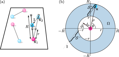
Any local MCMC move proposes a displacement of $\mathbf{x}_{1}$ or $\mathbf{x}_{2}$ from its present position along a line $\mathbf{l}$ of angle $\phi$ with the $x$-axis. If the final configuration has a dipole length with infinite $U$, the move is rejected. Such single-atom moves induce translations and rotations of the entire dipole. We need not consider explicit global MCMC translations or global rotations which, in the application to ECMC that we have in mind, are difficult to implement. Because of homogeneity, uniform translations of the dipole decouple from its rotations. We may thus set $\mathbf{x}_{1}=(0,0)$ and consider the relative position in polar coordinates: $\mathbf{x}=\mathbf{x}_{2}-\mathbf{x}_{1}=(\rho,\theta)$, with the dipole angle $\theta$. In equilibrium, $\mathbf{x}$ is uniformly distributed on the sample space $\Omega$, the two-dimensional ring of inner radius $r$ and outer radius $R$ centered at $(0,0)$ (see figure 1b). The uniform Euclidean distribution on $\Omega$ translates into a dipole-length distribution $\pi(\rho)=2\rho/\left[r^{2}\left(\eta^{2}-1\right)\right]$ for $\rho\in[r,R]$ with $\eta=R/r$, and a dipole-angle distribution for $\theta$ that is uniform in $(-\pi,\pi]$.

The sampling of the dipole $(\mathbf{x}_{1},\mathbf{x}_{2})$ may be tracked in the ring representation for $\mathbf{x}\in\Omega$, because any move of $\mathbf{x}_{2}$ corresponds to the identical move for $\mathbf{x}$, and any move of $\mathbf{x}_{1}$ yields an inverse move for $\mathbf{x}$. In both cases, the move is on a line $\mathbf{l}\ni\mathbf{x}$ of angle $\phi$ with the $x$-axis. We thus parameterize a direction of a local MCMC move by $\phi$. The trajectory of the dipole angle under slow direction sweeps is closely connected to the trajectory of the impact parameter

$$\lambda=\frac{\sin(\theta-\phi)\rho}{r},$$ (2)

which denotes the signed distance (in units of $r$) of $\mathbf{l}$ to the origin in a local MCMC move. In the reference frame where $\phi=0$, i.e., where $\mathbf{l}$ runs parallel to the $x$-axis, $\lambda$ is positive for $\mathbf{x}$ in the upper half plane and negative in the lower half plane. If $|\lambda|>1$, $\mathbf{l}\cap\Omega$ forms a single segment $\mathcal{S}$ that contains all accessible configurations. If $|\lambda|<1$, $\mathbf{l}\cap\Omega$ forms two such segments, namely $\mathcal{S}^{-}$ (to the left for $\phi=0$) and $\mathcal{S}^{+}$ (to the right) (see figure 1b). In realistic applications like, e.g., dense dipole systems, accepted local MCMC moves with $|\lambda|<1$ that jump from $\mathcal{S}^{-}$ to $\mathcal{S}^{+}$ are highly unlikely. We thus only consider local MCMC moves that remain within their respective segment ($\mathcal{S}$, $\mathcal{S}^{-}$ or $\mathcal{S}^{+}$) or, in other words, local MCMC moves that can be constructed from infinitesimal legal moves.

3 Direction-sweep MCMC

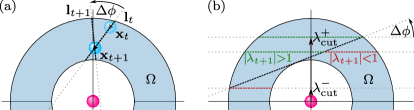
Local MCMC moves along one direction $\phi$ tend towards a restricted equilibrium among the accessible configurations in $\mathcal{S}$, $\mathcal{S}^{-}$ or $\mathcal{S}^{+}$. For the single two-dimensional dipole, the restricted-equilibrium limit can be reached in a single step by sampling the final position of the dipole in the segment that contains the starting position $\mathbf{x}$. This allows us to focus on the effects introduced by the choice of directions. In the following, one unit of MCMC time corresponds to one fixed direction. We therefore obtain the next position $\mathbf{x}_{t+1}$ as a direct uniform sample [25] in $\mathcal{S}$ for $|\lambda_{t}|>1$, and in $\mathcal{S}^{-}$ or in $\mathcal{S}^{+}$ (depending on the starting position $\mathbf{x}_{t}$) for $|\lambda_{t}|<1$. The direction is incremented by a constant value after each time step, that is, the line $\mathbf{l}_{t+1}$ goes through $\mathbf{x}_{t+1}$ with the new angle $\phi_{t+1}=\phi_{t}+\Delta\phi$ (for concreteness, we suppose $\Delta\phi>0$) (see figure 2a). The original (“collapsed”) reversible version of direction-sweep MCMC randomly samples the new angle from $\phi_{t+1}=\phi_{t}\pm\Delta\phi$ instead. In this case, detailed balance follows from the fact that both the choice of $\mathbf{x}_{t+1}$ from $\mathbf{x}_{t}$, and of $\phi_{t+1}$ from $\phi_{t}$ are reversible.

• 

Figure 2: Direction-sweep MCMC with directions $\phi_{t+1}-\phi_{t}=\Delta\phi$. (a): Lines $\mathbf{l}_{t}\ni\mathbf{x}_{t}$ and $\mathbf{l}_{t+1}$ intersect at $\mathbf{x}_{t+1}$. (b): A large impact parameter ($|\lambda_{t}|>\lambda^{+}_{\text{cut}}$) leads to $|\lambda_{t+1}|>1\quad\forall\mathbf{x}_{t+1}\in\mathbf{l}_{t}$. Likewise, a small impact parameter ($|\lambda_{t}|<\lambda^{-}_{\text{cut}}$) leads to $|\lambda_{t+1}|<1\quad\forall\mathbf{x}_{t+1}\in\mathbf{l}_{t}$. Otherwise, if $\lambda^{-}_{\text{cut}}<|\lambda_{t}|<\lambda^{+}_{\text{cut}}$, the value of $\mathbf{x}_{t+1}$ determines whether $|\lambda_{t+1}|>1$ or $|\lambda_{t+1}|<1$.

Because of the $\pi$-periodicity of the directions, a given value of $\Delta\phi$ and the starting direction $\phi_{0}$ imply a set of directions $\mathcal{D}=\{\phi_{t}\}$ that contains all possible directions of a simulation. We only consider finite direction sets $\mathcal{D}$ for simplicity. Direction-sweep MCMC is a non-reversible lifting of reversible local MCMC with an augmented (lifted) sample space $\Omega\times\mathcal{D}$. The lifted stationary distribution depends on $\phi$: $\pi(\mathbf{x})\mapsto\pi(\mathbf{x},\phi)$, with $\sum_{\phi}\pi(\mathbf{x},\phi)=\pi(\mathbf{x})$ (see [26, 16] for definitions). We will show below that $\pi(\mathbf{x},\phi)$ is proportional to $\pi(\mathbf{x})$ for the sequential direction sweep. In order to converge towards the stationary distribution $\pi$, the direction-sweep MCMC algorithm must satisfy the global-balance condition:

$$\pi(\mathbf{x}_{t+1},\phi_{t+1})=\sum_{\mathbf{x}_{t},\phi_{t}}\pi(\mathbf{x}_{t},\phi_{t})\,p[(\mathbf{x}_{t},\phi_{t})\rightarrow(\mathbf{x}_{t+1},\phi_{t+1})],$$ (3)

where $p(a\rightarrow b)$ denotes the transition probability between the (lifted) configurations $a$ and $b$.

As explained, any move from $t$ to $t+1$ is composed of two parts. In the first part, the lifting variable is fixed ($\phi_{t+1}=\phi_{t}=\phi$) while a new position $\mathbf{x}_{t+1}$ is directly sampled among the accessible configurations given $\mathbf{x}_{t}$ and $\phi_{t}$. This restricted MCMC algorithm satisfies global balance for the given direction $\phi$ by construction, that is, $\pi(\mathbf{x}_{t+1},\phi)=\sum_{\mathbf{x}_{t}}\pi(\mathbf{x}_{t},\phi)\,p[(\mathbf{x}_{t},\phi)\rightarrow(\mathbf{x}_{t+1},\phi)]$. This yields specifically $\pi(\mathbf{x}_{t+1},\phi)=\pi(\mathbf{x}_{t},\phi)$ for the simple dipole model with its uniform $\pi$. In the second part of the move, the position $\mathbf{x}$ remains fixed and only the direction is incremented by $\Delta\phi$:

$$\pi(\mathbf{x},\phi_{t+1})=\sum_{\phi_{t}}\pi(\mathbf{x},\phi_{t})\,p[\phi_{t}\to\phi_{t+1}]=\pi(\mathbf{x},\phi_{t+1}-\Delta\phi).$$ (4)

For a finite direction set, and taking into account the periodicity of directions, this establishes that the lifted stationary distribution $\pi(\mathbf{x},\phi)$ is independent of $\phi$. The first and second parts together establish the validity of the global-balance condition in (3). For the two-dimensional dipole model, direction-sweep MCMC is aperiodic and irreducible for any choice of two or more directions. The independence of the stationary distribution $\pi(\mathbf{x},\phi)$ with respect to the lifting variable is a general property of lifted MCMC [16].

For small $\Delta\phi$, direction-sweep MCMC features two cutoff impact parameters $\lambda^{+}_{\text{cut}}$ and $\lambda^{-}_{\text{cut}}$:

$$\lambda^{\pm}_{\text{cut}}=\cos(\Delta\phi)\pm\sqrt{(\eta^{2}-1)\sin^{2}(\Delta\phi)}.$$ (5)

Here, $\lambda^{+}_{\text{cut}}$ exists for $\cos(\Delta\phi)>1/\eta$, and $\lambda^{-}_{\text{cut}}$ for $\cos(\Delta\phi)>(\eta^{2}-2)/\eta^{2}$. For a fixed value of $\eta$, $\lambda^{\pm}_{\text{cut}}$ both exist in the limit $\Delta\phi\to 1$ and approach $1$ as $\lambda^{\pm}_{\text{cut}}\to 1^{\pm}$. The interval $[\lambda^{-}_{\text{cut}},\lambda^{+}_{\text{cut}}]$ is a separation layer for the impact parameter $\lambda$ because $|\lambda_{t}|>\lambda^{+}_{\text{cut}}$ implies $|\lambda_{t+1}|>1$, whereas $|\lambda_{t}|<\lambda^{-}_{\text{cut}}$ implies $|\lambda_{t+1}|<1$ (see figure 2b).

4 Equilibrium Properties

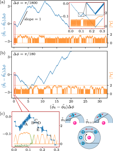
For small $\Delta\phi>0$, direction-sweep MCMC simulations of the single two-dimensional dipole yield trajectories of $\tilde{\theta}_{t}$, the rolled-out dipole angle (not wrapped back into a $2\pi$ interval), with alternating positive and negative rotations. The positive rotations fluctuate around their average of $\Delta\phi$ per time step, so that the trajectory of $(\tilde{\theta}_{t}-\tilde{\theta}_{0})\Delta\phi$ vs $(\tilde{\phi}_{t}-\tilde{\phi}_{0})\Delta\phi$ has an average unit slope ($\tilde{\phi}_{t}$ is the rolled-out direction: $\tilde{\phi}_{t}-\tilde{\phi}_{0}=t\Delta\phi$). The negative rotations exhibit, in contrast, intermittent sharp decreasing steps and constant plateaus (see figure 3).

• 

Figure 3: Trajectories of $(\tilde{\theta}_{t}-\tilde{\theta}_{0})\Delta\phi$ (blue, upper) and of $|\lambda_{t}|$ (yellow, lower) vs. $(\tilde{\phi}_{t}-\tilde{\phi}_{0})\Delta\phi$ for $\eta=2$. (a): $\Delta\phi=\pi/1800$. The inset shows the initial trajectories. (b): $\Delta\phi=\pi/180$. (c): Initial trajectories for $\Delta\phi=\pi/180$, with “excursions” (upper right) and “zigzags” (lower right).

We will show that the trajectory of $\tilde{\theta}_{t}$ depends on that of the impact parameter $\lambda_{t}$ (see sections 4.1 and 4.2). Therefore, we first treat the trajectory of $\lambda_{t}$ that may be described through drift and diffusion terms. The current value of the impact parameter $\lambda_{t}$ is a function of the position $\mathbf{x}_{t}$ and direction $\phi_{t}$ (for fixed system parameters). Direction-sweep MCMC algorithm then uniformly samples $\mathbf{x}_{t+1}$ on the segment that also contains $\mathbf{x}_{t}$. The subsequent increment of the direction by $\Delta\phi$ linearly maps $\mathbf{x}_{t+1}$ onto the impact parameter $\lambda_{t+1}$. The position $\mathbf{x}_{t+1}$, given $\mathbf{x}_{t}$, is a random variable, and so is $\lambda_{t+1}$. Its conditional expectation is

$$\mathbb{E}\,(\lambda_{t+1}|\lambda_{t})=\cases{\lambda_{t}\cos\!\,\Delta\phi\mp A_{t}\sin\!\,\Delta\phi&if $|\lambda_{t}|<1$; $\mathbf{x}_{t}\in\mathcal{S}^{\pm}$,\\ \lambda_{t}\cos\!\,\Delta\phi\hphantom{\mp A_{t}\sin\!\,\Delta\phi s}&if $|\lambda_{t}|>1$,}$$ (6)

where $A_{t}=(B_{t}+C_{t})/2$ with $B_{t}=\sqrt{\eta^{2}-\lambda_{t}^{2}}$ and $C_{t}=\sqrt{1-\lambda_{t}^{2}}$. The variance of $\lambda_{t+1}$ is

$$\sigma^{2}(\lambda_{t+1}|\lambda_{t})=\cases{\frac{1}{12}\sin^{2}\left(\Delta\phi\right)\left(B_{t}-C_{t}\right)^{2}&if $|\lambda_{t}|<1$,\\ \frac{1}{3}\sin^{2}\left(\Delta\phi\right)B_{t}^{2}&if $|\lambda_{t}|>1$.}$$ (7)

Equations (6) and (7) are the expectation and variance of a uniform distribution of $\lambda_{t+1}$.

For small $\Delta\phi>0$, the trajectories of direction-sweep MCMC are exactly equivalent to those of a Gaussian process:

$$\lambda_{t+1}=\lambda_{t}+[\mathbb{E}\,(\lambda_{t+1}|\lambda_{t})-\lambda_{t}]+\sqrt{\sigma^{2}(\lambda_{t+1}|\lambda_{t})}\,w_{t},$$ (8)

where $w_{t}$ samples a standard normal distribution. For small $\Delta\phi$, the fluctuation term $\sqrt{\sigma^{2}(\lambda_{t+1}|\lambda_{t})}$ is proportional to $\Delta\phi$. The drift $\mathbb{E}\,(\lambda_{t+1}|\lambda_{t})-\lambda_{t}$ is proportional to $(\Delta\phi)^{2}$ for $|\lambda|>1$ and proportional to $\Delta\phi$ for $|\lambda|<1$. This leads to distinctive dynamics for $|\lambda|>1$ and for $|\lambda|<1$,

4.1 Excursions ($|\lambda|>1$)

For $|\lambda_{t}|>1$, (8) becomes

$$\lambda_{t+1}=\lambda_{t}-\frac{\lambda_{t}}{2}(\Delta\phi)^{2}+\sqrt{\frac{1}{3}B_{t}^{2}(\Delta\phi)^{2}}\,w_{t}$$ (9)

in the limit of small $\Delta\phi$. This equation agrees with the discrete-time Langevin equation

$$\lambda_{t+1}=\lambda_{t}+D^{(1)}(\lambda_{t},t_{t})\tau+\sqrt{2D^{(2)}(\lambda_{t},t_{t})\tau}\,w_{t},$$ (10)

where the discrete times $t_{t}$ are separated by the time step $\tau$, and $D^{(1)}$ and $D^{(2)}$ are the Kramers–Moyal expansion coefficients of the time-dependent probability distribution of $\lambda$ that correspond to drift and diffusion, respectively (see [27, eq. (3.138)]). For $|\lambda|>1$, the impact parameter thus performs an “excursion”, a random walk in the quantity $\tau=(\Delta\phi)^{2}$. Such an excursion corresponds to a total number of time steps that scales as $\sim\text{const}/(\Delta\phi)^{2}$. As each time step increases the direction by $\Delta\phi$, this increases the rolled-out direction by an amount that diverges as $\sim\text{const}/\Delta\phi$. The excursions with $|\lambda|>1$ for different $\Delta\phi$ therefore become similar if the trajectory of the impact parameter is recorded as a function of $(\tilde{\phi}_{t}-\tilde{\phi}_{0})\Delta\phi$ (see figure 3a and b).

During the excursion, $\mathbf{x}_{t}$ follows the rotation of the direction in steps of $\Delta\phi$ (see figure 3c). Thus, the difference in the rolled-out dipole angle during an excursion diverges as $\sim\text{const}/\Delta\phi$. For $\Delta\phi>0$, this is evidenced by the unit slope of the increasing parts of the trajectories of $(\tilde{\theta}_{t}-\tilde{\theta}_{0})\Delta\phi$ as a function of $(\tilde{\phi}_{t}-\tilde{\phi}_{0})\Delta\phi$ (see figure 3a and b, again).

4.2 Zigzags ($|\lambda|<1$)

For $|\lambda_{t}|<1$, the fluctuations in (7) are negligible for small $\Delta\phi$ and the Gaussian process of (8) approaches its deterministic limit:

$$\Delta\lambda=\lambda_{t+1}-\lambda_{t}=\mp\frac{\sqrt{\eta^{2}-\lambda_{t}^{2}}+\sqrt{1-\lambda_{t}^{2}}}{2}\,\Delta\phi,$$ (11)

where the negative sign on the right-hand side is for $\mathbf{x}_{t}\in\mathcal{S}^{+}$, and the positive sign for $\mathbf{x}_{t}\in\mathcal{S}^{-}$. For small $\Delta\phi$, this becomes a non-linear differential equation whose solution (up to an integration constant) is

$$\phi(\lambda)=\pm\frac{\arcsin(\lambda)-\eta^{2}\arcsin(\lambda/\eta)+\lambda[C(\lambda)-B(\lambda)]}{\eta^{2}-1},$$ (12)

where $B(\lambda)=\sqrt{\eta^{2}-\lambda^{2}}$ and $C(\lambda)=\sqrt{1-\lambda^{2}}$. The numerical trajectories (for $|\lambda|<1$) reproduce the exact solution of (12) (see figure 3c).

For small $\Delta\phi>0$, if $\mathbf{x}$ enters the segment $\mathcal{S}^{+}$ with unit impact parameter $\lambda=1$, $\lambda$ will decrease at every step until $\lambda=-1$. In $\mathcal{S}^{-}$, the impact parameter likewise increases from $\lambda=-1$ to $\lambda=1$. This trapped deterministic motion creates one “zigzag” in the trajectory of $|\lambda|$. The total change of the rolled-out direction $\Delta\tilde{\phi}_{\text{ZZ}}$ during such a zigzag is given by

$$\Delta\tilde{\phi}_{\text{ZZ}}=\frac{2\eta^{2}\mathrm{arccsc}(\eta)+2\sqrt{\eta^{2}-1}-\pi}{\eta^{2}-1},$$ (13)

and is always smaller than $\pi$. In a reference frame with $\phi_{t}=0$, (which is rotated by $-\Delta\phi$ at every time step), $\mathbf{x}$ performs a negative rotation (see the trajectory from $B$ to $D$ in figure 3c), and thus follows the rotation of the system. Therefore, the rolled-out dipole angle $\tilde{\theta}_{t}$ remains roughly constant, leading to a plateau in the non-rotating reference frame. For $\lambda_{t}=0$, the dipole angle $\tilde{\theta}_{t}$ is independent of the precise position $\mathbf{x}_{t}$ on its segment. At the center of each plateau, the fluctuations of $\tilde{\theta}_{t}$ thus vanish even at finite $\Delta\phi$ (see point $C$ in figure 3c).

Since the total change of the rolled-out direction $\Delta\tilde{\phi}_{\text{ZZ}}$ in (13) is independent of $\Delta\phi$, the zigzags in the trajectories of $|\lambda_{t}|$ for different (small) values of $\Delta\phi$ are similar if plotted as a function of $\tilde{\phi}_{t}-\tilde{\phi}_{0}$, but ever steeper as a function of $(\tilde{\phi}_{t}-\tilde{\phi}_{0})\Delta\phi$ (see figure 3a and b).

4.3 Interplay of excursions and zigzags

• 

Figure 4: Distributions $\pi(\tilde{\theta}_{t+N_{t}}-\tilde{\theta}_{t})$ for $\eta=1.1$ and $\Delta\phi=\pi/180$. (a): $N_{t}=1$. (b): Distributions for moderate $N_{t}$. (c): Rescaled large-$N_{t}$ distributions compared to a Gaussian distribution.

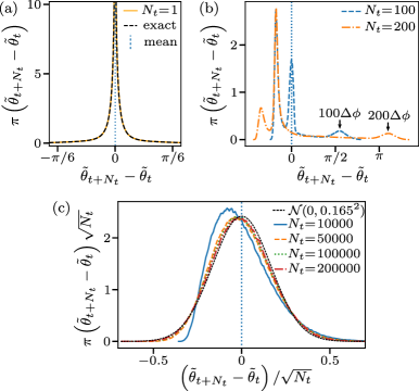
After one rapid motion from $\lambda=1$ to $\lambda=-1$ or vice versa, the trajectory may switch segments to continue at $|\lambda|<1$, adding one more leg to the negative-rotation zigzag of $\lambda_{t}$ (or two legs to the zigzag of $|\lambda_{t}|$ in figure 3c). The trajectory may also switch to an excursion with $|\lambda|>1$, that is, to a positive rotation of the rolled-out dipole angle $\tilde{\theta}$. The time (number of steps) of an excursion scales as $\sim\text{const}/(\Delta\phi)^{2}$ whereas the time of one zigzag is shorter by factor of $\Delta\phi$ as it scales as $\sim\text{const}/\Delta\phi$. Nevertheless, positive and negative rotations balance, and the expectations $\mathbb{E}\,(\tilde{\theta}_{t+N_{t}}-\tilde{\theta}_{t})$ are zero for all values of $N_{t}$. This holds for a single move ($N_{t}=1$) because $\pi(\tilde{\theta}_{t+1}-\tilde{\theta}_{t})$ is symmetric in consequence of the detailed balance of the move from $t$ to $t+1$ (see figure 4a). For $N_{t}>1$, $\tilde{\theta}_{t+N_{t}}-\tilde{\theta}_{t}=\tilde{\theta}_{t+N_{t}}-\tilde{\theta}_{t+N_{t}-1}+\dots+\tilde{\theta}_{t+1}-\tilde{\theta}_{t}$ yields

$$\mathbb{E}\left(\tilde{\theta}_{t+N_{t}}-\tilde{\theta}_{t}\right)=\mathbb{E}\left(\tilde{\theta}_{t+N_{t}}-\tilde{\theta}_{t+N_{t}-1}\right)+\dots$$

$$+\mathbb{E}\left(\tilde{\theta}_{t+2}-\tilde{\theta}_{t+1}\right)+\mathbb{E}\left(\tilde{\theta}_{t+1}-\tilde{\theta}_{t}\right)=0,$$ (14)

because the expectation of a sum of (possibly dependent) random variables equals the sum of expectations. The distribution $\pi(\tilde{\theta}_{t+N_{t}}-\tilde{\theta}_{t})$, although it is of zero expectation, can be highly asymmetric (see figure 4b). For $N_{t}\lesssim\text{const}/(\Delta\phi)^{2}$, the distribution peaks for large $\tilde{\theta}$ that corresponds to trajectories that remain on long excursions. For $N_{t}\gg\text{const}/(\Delta\phi)^{2}$, the distribution approaches a Gaussian and becomes again symmetric because the large number of steps allows excursions and zigzags to compensate in a single trajectory (see figure 4c). The vanishing of $\mathbb{E}\,(\tilde{\theta}_{t+N_{t}}-\tilde{\theta}_{t})$ implies that there are $\mathcal{O}(1/\Delta\phi)$ zigzags for each excursion. Microscopically, this can be understood through the existence of the cutoff value $\lambda^{+}_{\text{cut}}$ (see (5) and figure 2b). If $|\lambda_{t}|>\lambda^{+}_{\text{cut}}$, the next value of the impact parameter $|\lambda_{t+1}|>1$; in contrast, a current value of the impact parameter $1<|\lambda_{t}|<\lambda^{+}_{\text{cut}}$ may either produce $|\lambda_{t+1}|>1$ or $|\lambda_{t+1}|<1$. In the latter case, $\mathbf{x}$ gets trapped in its corresponding segment.

5 Approach to equilibrium

The trajectory of the dipole in its sample space $\Omega=\{(\rho,\theta)\}$ is characterized by persistent negative and positive rotations. In order to quantify the approach to equilibrium of direction-sweep MCMC, we consider mixing times [2, 28]

$$t_{\text{mix}}(\varepsilon)=\min\{t:d(t)\leq\varepsilon\},$$ (15)

where $d(t)$ is the total variation distance (TVD) between the stationary distribution $\pi$ and the probability distribution $P^{t}(\overline{\mathbf{x}}_{0},\cdot)$ at time $t$ obtained by starting from the most unfavorable lifted initial configuration $\overline{\mathbf{x}}_{0}$:

$$d(t) =\max_{\overline{\mathbf{x}}_{0}}\,||P^{t}(\overline{\mathbf{x}}_{0},\cdot)-\pi||_{\text{TVD}}$$ (16)

$$=\max_{\overline{\mathbf{x}}_{0}}\,\frac{1}{2}\int\mathrm{d}\overline{\mathbf{x}}\,|P^{t}(\overline{\mathbf{x}}_{0},\overline{\mathbf{x}})-\pi(\overline{\mathbf{x}})|.$$ (17)

The time $t_{\text{mix}}=t_{\text{mix}}(1/4)$ is defined as the mixing time. For $\varepsilon<1/4$, $t_{\text{mix}}(\varepsilon)$ is bounded through $t_{\text{mix}}$,

$$t_{\text{mix}}(\varepsilon)\leq\lceil\log_{2}\varepsilon^{-1}\rceil\,t_{\text{mix}},$$ (18)

showing that the mixing process is exponential [2].

We checked numerically for the dipole that the same $\overline{\mathbf{x}}_{0}$ maximizes the TVD for $\varepsilon$ in the neighborhood of $1/4$ and determine $t_{\text{mix}}$ via the time $t_{\text{mix}}(\overline{\mathbf{x}}_{0})$:

$$t_{\text{mix}}(\overline{\mathbf{x}}_{0})=\min\{t:||P^{t}_{\theta}(\overline{\mathbf{x}}_{0},\cdot)-\pi_{\theta}||_{\text{TVD}}\leq 1/4\}.$$ (19)

The maximum of $t_{\text{mix}}(\overline{\mathbf{x}}_{0})$ over the initial configurations $\overline{\mathbf{x}}_{0}$ then yields $t_{\text{mix}}$ (by doing so, we effectively interchanged the $\min$ in (15) with the $\max$ in (17)). Due to the rotational invariance of the ring system, $t_{\text{mix}}(\overline{\mathbf{x}}_{0})$ only depends on the angle difference $\theta_{0}-\phi_{0}$. We thus set $\phi_{0}=0$ and consider $t_{\text{mix}}(\rho_{0},\theta_{0})$, which we determine numerically by running $100000$ simulations that all start from $\overline{\mathbf{x}}_{0}=(\rho_{0},\theta_{0})$. At each time step $t$, we use these simulations to determine $P^{t}_{\theta}(\overline{\mathbf{x}}_{0},\cdot)$ and its TVD with $\pi$. The evaluation of the TVD requires in our case the evaluation of a two-dimensional integral over $\Omega$. However, since $\rho$ relaxes very fast, we approximate it by the one-dimensional integral over $\theta$.

5.1 Identifying unfavorable initial configurations

For small $\Delta\phi>0$, two unfavorable initial configurations stand out. First, trajectories with $\lambda_{0}=1$ and $\overline{\mathbf{x}}_{0}\in\mathcal{S}^{+}$ (or $\lambda_{0}=-1$ and $\overline{\mathbf{x}}_{0}\in\mathcal{S}^{-}$) always start with a deterministic zigzag until $\lambda_{t}=-1$ (or $\lambda_{t}=1$). At the time $t$ after this first zigzag, the probability distribution $P^{t}_{\theta}(\overline{\mathbf{x}}_{0},\cdot)$ is therefore strongly peaked and produces a large TVD in (17). Thereafter, different trajectories either continue with more zigzags or else with an excursion, which then flattens $P^{t}_{\theta}(\overline{\mathbf{x}}_{0},\cdot)$. Second, a trajectory from $|\lambda_{0}|=\eta$ starts with an excursion and $P^{t}_{\theta}(\overline{\mathbf{x}}_{0},\cdot)$ thus peaks at $\theta_{t}=t\Delta\phi$. Once the random walk in $|\lambda_{t}|$ reaches $\lambda^{+}_{\text{cut}}$, the distribution $P^{t}_{\theta}(\overline{\mathbf{x}}_{0},\cdot)$ starts to flatten. The most unfavorable initial configuration among these two depends on $\eta$. For $\eta\rightarrow 1$, we find that starting the trajectory with a zigzag is the most unfavorable initial state, whereas starting the trajectory with an excursion is most unfavorable for larger $\eta$ (see figure 5a and b). This can be understood by the fact that the number of time steps in a zigzag increases as $\eta\to 1$ (see (13)), whereas the difference $\eta-\lambda^{+}_{\text{cut}}$ that the impact parameter has to overcome in the initial excursion decreases (see (5)).

• 

Figure 5: Mixing times $t_{\text{mix}}(\overline{\mathbf{x}}_{0}=(\rho_{0},\theta_{0}))$ for different values of $\eta$ and $\Delta\phi$.

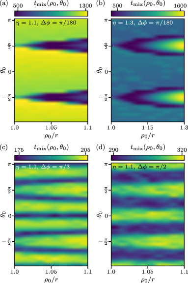
For large $\Delta\phi$, the random walk of $\lambda_{t}$ is no longer described in terms of excursions and zigzags, and the initial configuration does not strongly influence $t_{\text{mix}}(\overline{\mathbf{x}}_{0})$, except for values of $\Delta\phi$ that correspond to small direction sets $\mathcal{D}$. Then $t_{\text{mix}}(\rho_{0},\theta_{0})$ is roughly periodic in $\theta_{0}$ (see figure 5c and d). For $\Delta\phi=\pi/2$, this may be due to the fact that with $\theta_{0}\in\{-\pi/2,0,\pi/2,\pi\}$ one of the two alternating directions hardly modifies $\theta_{t}$ during the initial part of the trajectory.

5.2 Mixing Time

We now systematically study $t_{\text{mix}}$ for direction-sweep MCMC as a function of the direction set $\mathcal{D}$. We compare it with the reversible version that samples $\phi_{t+1}$ randomly from $\mathcal{D}$ (random discrete MCMC), and also with reversible MCMC with continuous directions $\Delta\phi=\mathrm{ran}(0,\pi)$ (random continuous MCMC). Both versions satisfy detailed balance.

Several properties stand out (see figure 6a). First, the mixing time is very sensitive to the size of $\mathcal{D}$ regardless of whether its elements are accessed sequentially or randomly. For a thin ring ($\eta\to 1$), the mixing time $t_{\text{mix}}$ shows characteristic peaks for small direction sets $\mathcal{D}$. The height of these peaks (for not too large set sizes $|\mathcal{D}|$) is proportional to $1/|\mathcal{D}|$. This yields a particularly large mixing time for $\Delta\phi=\pi/2$ where $|\mathcal{D}|=2$.

• 

Figure 6: Mixing times $t_{\text{mix}}$ of direction-sweep MCMC for different $\Delta\phi$. (a): $t_{\text{mix}}$ at $\eta=1.005$ compared to mixing times of random discrete and continuous MCMC. (b): Optimal speedup with respect to $\Delta\phi=\pi/2$ and to random continuous MCMC. (c): $t_{\text{mix}}$ of direction-sweep MCMC compared to that of random continuous MCMC for $\eta\gtrsim 1$. The line labeling is the same as in (a).

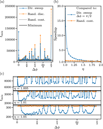
Second, we find that sweeping through the elements of $\mathcal{D}$ is generically better than randomly sampling the direction from $\mathcal{D}$, except for $\Delta\phi\to 0$ where the sweeps are too slow and the mixing time diverges. For small $|\mathcal{D}|$, this benefit of direction-sweep MCMC is easily understood by the non-vanishing probability of repeated (redundant) moves in the same direction that only appear in random discrete MCMC.

For all considered values of $\eta$, we find that direction-sweep MCMC with appropriate $\Delta\phi$ is faster than random continuous MCMC and, in particular, as direction-sweep MCMC with $\Delta\phi=\pi/2$ (see figure 6b). The speedup compared to the choice $\Delta\phi=\pi/2$ is large, and it appears to diverge as $\eta\to 1$. This may render the non-reversible scheme especially promising for dipolar particles in ECMC where up to now $\Delta\phi=\pi/2$ was always chosen. We confirm that the smallest mixing time in direction-sweep MCMC is indeed reached for small $\Delta\phi$, that is, for the peculiar trajectories discussed in section 4. This, in our model, can of course only be observed for $\eta\to 1$ because the speedup for small $\Delta\phi$ is cut off by the divergence of $t_{\text{mix}}$ for $\Delta\phi\to 0$.

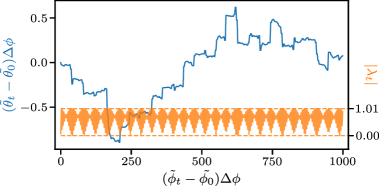
Finally, we find that direction-sweep MCMC is usually faster than the random continuous MCMC even for large values of $\Delta\phi$, except when $|\mathcal{D}|$ is very small (see figure 6c, large angles $\Delta\phi$ give small direction sets only if $\Delta\phi/(2\pi)$ is a simple fraction). The trajectories remain very regular for generic $\Delta\phi$. They feature intriguing patterns for the impact parameter $\lambda_{t}$ and the rolled-out dipole angle $\tilde{\theta}_{t}$, that require further study (see figure 7).

• 

Figure 7: Trajectories of $(\tilde{\theta}_{t}-\tilde{\theta}_{0})\Delta\phi$ (blue, upper) and of $|\lambda_{t}|$ (yellow, lower) vs. $(\tilde{\phi}_{t}-\tilde{\phi}_{0})\Delta\phi$ for $\eta=1.01$ and $\Delta\phi=85\,\pi/180$.

6 Conclusion

We have discussed a non-reversible MCMC algorithm for particle systems that sweeps through the direction of motion, rather than to sample directions randomly. For a single two-dimensional dipole, we proved in a local-equilibrium limit that direction-sweep MCMC induces persistent dipole rotations with a total rolled-out angle that diverges as the direction sweep becomes slower. Persistent rotation takes place in both senses, and the two exactly compensate to zero net rotation.

Direction-lifted MCMC (of which direction-sweep MCMC is a special case) remains valid for general $N$-body problems. It preserves the independence of the lifted stationary distribution from the lifting variable [16] even if the thermalization condition at fixed lifting variable is dropped. Real-world direction-lifted MCMC may go to much smaller values of $\Delta\phi$ than the single dipole, simply because mixing times will be much larger in applications. It will thus be fascinating to understand the usefulness of direction lifting for applications such as polymer physics, and also in systems of long-range interacting extended molecules at the core of the JeLLyFysh project [21]. More generally, our model illustrates that non-reversibility profoundly changes the basic properties of local MCMC algorithms, in the same way as out-of-equilibrium statistical physics is fundamentally different from its equilibrium counterpart.

References

- [1] Metropolis N, Rosenbluth A W, Rosenbluth M N, Teller A H and Teller E 1953 J. Chem. Phys. 21 1087–1092
- [2] Levin D A, Peres Y and Wilmer E L 2008 Markov Chains and Mixing Times (American Mathematical Society)
- [3] O’Keeffe C J and Orkoulas G 2009 J. Chem. Phys. 130 134109
- [4] Kapfer S C and Krauth W 2017 Phys. Rev. Lett. 119(24) 240603
- [5] Lei Z and Krauth W 2018 EPL 124 20003
- [6] Ren R, O’Keeffe C J and Orkoulas G 2007 Mol. Phys. 105 231–238
- [7] Berg B A 2004 Markov Chain Monte Carlo simulations and their statistical analysis: with web-based Fortran code (World Scientific) ISBN 9789812389350
- [8] Diaconis P, Holmes S and Neal R M 2000 Ann. Appl. Probab. 10 726–752
- [9] Suwa H and Todo S 2010 Phys. Rev. Lett. 105(12) 120603
- [10] Turitsyn K S, Chertkov M and Vucelja M 2011 Physica D 240 410 – 414 ISSN 0167-2789
- [11] Fernandes H C and Weigel M 2011 Comput. Phys. Commun. 182 1856–1859 ISSN 0010-4655
- [12] Bierkens J, Bouchard-Côté A, Doucet A, Duncan A B, Fearnhead P, Lienart T, Roberts G and Vollmer S J 2018 Stat. Probab. Lett. 136 148–154
- [13] Bierkens J and Roberts G 2017 Ann. Appl. Probab. 27 846–882
- [14] Bernard E P, Krauth W and Wilson D B 2009 Phys. Rev. E 80(5) 056704
- [15] Michel M, Kapfer S C and Krauth W 2014 J. Chem. Phys. 140 054116
- [16] Krauth W 2021 Frontiers in Physics 9 229
- [17] Klement M and Engel M 2019 J. Chem. Phys. 150 174108
- [18] Michel M, Durmus A and Sénécal S 2020 J. Comput. Graph. Stat. 29 689–702
- [19] Weigel R F B Equilibration of Orientational Order in Hard Disks via Arcuate Event-Chain Monte Carlo Master thesis, Friedrich-Alexander-Universität Erlangen-Nürnberg, 2018 URL https://theorie1.physik.uni-erlangen.de/research/theses/2018-ma-roweigel.html
- [20] Faulkner M F, Qin L, Maggs A C and Krauth W 2018 J. Chem. Phys. 149 064113
- [21] Höllmer P, Qin L, Faulkner M F, Maggs A C and Krauth W 2020 Comput. Phys. Commun. 253 107168
- [22] Wu Y, Tepper H L and Voth G A 2006 J. Chem. Phys. 124 024503
- [23] Müller D, Kampmann T A and Kierfeld J 2020 Scientific Reports 10
- [24] Kampmann T A, Müller D, Weise L P, Vorsmann C F and Kierfeld J 2021 Frontiers in Physics 9 635886
- [25] Krauth W 2006 Statistical Mechanics: Algorithms and Computations (Oxford University Press)
- [26] Chen F, Lovász L and Pak I 1999 Proceedings of the 17th Annual ACM Symposium on Theory of Computing 275
- [27] Risken H 1989 The Fokker-Planck Equation (Springer Berlin Heidelberg)
- [28] Diaconis P 2011 J. Stat. Phys. 144 445 ISSN 1572-9613