Electron-magnon spin conversion and magnonic spin pumping in antiferromagnet/heavy metal heterostructure

Abstract

We study the exchange between electron and magnon spins at the interface of an antiferromagnet and a heavy metal at finite temperatures. The underlying physical mechanism is based on spin torque associated with the creation/annihilation of thermal magnons with right-hand and left-hand polarization. The creation/annihilation process depends strongly on the relative orientation between the polarization of the electron and the magnon spins. For a sufficiently strong spin transfer torque (STT), the conversion process becomes nonlinear, generating a nonzero net spin pumping current in the AFM that can detected in the neighboring metal layer. Applying an external magnetic field renders possible the manipulation of the STT driving thermal spin pumping. Our theoretical results are experimentally feasible and are of a direct relevance to antiferromagnet-based spintronic devices.

I Introduction

Electronic and magnonic spin currents are central to spintronics Žutić et al. (2004); Chumak et al. (2015); Wolf et al. (2001); Ohno (2010); Sinova et al. (2015); Heinrich et al. (2011). Electronic spin current is generated for instance due to the spin Hall effect (SHE) in a non-magnetic metal layerHirsch (1999); Valenzuela and Tinkham (2006); Sinova et al. (2015); Kato et al. (2004), or through the oscillation of magnetization in a ferromagnetic layer (spin pumping) Tserkovnyak et al. (2005); Saitoh et al. (2006); Sandweg et al. (2011); Ando et al. (2011). The magnonic spin current, meaning a flux of non-equilibrium magnons results from an applied temperature gradient, microwave field, or due to electronic spin-transfer torque Chumak et al. (2015); Uchida et al. (2010); Chumak et al. (2012); Kajiwara et al. (2010); Wang et al. (2017); Chotorlishvili et al. (2019); Wang et al. (2012). Spin currents in antiferromagnets (AFMs) are also highly interesting for AFM spintronics Jungwirth et al. (2016); Gomonay and Loktev (2014); Baltz et al. (2018); Gomonay et al. (2018); Jungfleisch et al. (2018). Several spin transport phenomena, including SHE, spin Seebeck effect, N${\rm\acute{e}}$el spin-orbit torque were reported and their potential for applications were discussed in AFMs Jungwirth et al. (2016); Gomonay and Loktev (2014); Baltz et al. (2018); Gomonay et al. (2018); Jungfleisch et al. (2018); Park et al. (2011); Rezende et al. (2016a, b); Wadley et al. (2016); Wu et al. (2016); Chen et al. (2018). Of a particular interest is the behavior of a magnonic spin current flowing from a ferromagnet (FM) across an insulating AMF layer Wang et al. (2014); Rezende et al. (2016b); Lin et al. (2016); Moriyama et al. (2015); Li et al. (2020); Vaidya et al. (2020); Lebrun et al. (2018); Dabrowski et al. (2020), which offers a way for integration of magnonic spintronic and AFM devices, and allowing to act on the AFM by exciting the FM layer Rezende et al. (2016b).

The present work proves that, due to finite temperature magnonic excitations in AFM, the electronic spin-current in heavy metal (HM) can traverse through the insulating AFM layer. In our model, not FM, but the AFM layer plays the role of the spin-current tunnel junction. We sandwich the AFM layer between two HM layers, meaning we consider HM / insulating AFM / HM heterostructure. At finite temperatures, the electronic spin current creates (annihilates) thermal magnons with spin polarization opposite (parallel) to the polarization of the electron spin. Thus, spins of the electrons from the HM layer are efficiently converted to AFM magnons. The induced magnon spins are further delivered to the second HM layer, and eventually are converted back to the electron spin current via the spin pumping effect. The effectiveness of the spin transport via magnons depends on the electronic spin current and on the external magnetic field.

The paper is organized as follows: In section II we specify the model, in section III we analyze the polarization of magnons and derive the magnon eigenmodes, in section IV we explore the effect of STT. The thermal and spin pumping effects we discuss in section V. In sections VI and VII we discuss the effect of external magnetic fields and conclude with section VIII.

II Theoretical model

The structure considered in this study is shown in Fig. 1(a). The AFM layer is sandwiched between two HMs. A charge current with density $J_{\rm Pt}$ passes through one metal and induces a transversal spin current due to the spin Hall effect. The electronic spin current is converted into a magnonic spin current at the AFM/HM interface via the SHE-based spin-transfer torque (STT) Chen et al. (2018); Cheng et al. (2016). The magnonic spin current is detected in the second metal via the spin pumping effect Johansen and Brataas (2017); Li et al. (2020); Vaidya et al. (2020); Chotorlishvili et al. (2015).

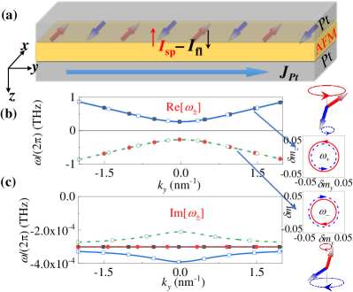
Figure 1: (a) Schematics of the studied heterostructure. The insulating antiferromagnet is sandwiched between two HMs (here, Pt). An charge current with density $J_{\rm{\rm Pt}}$ flows in one of the metal layer. The pure electron spin current generated through the spin Hall effect is denoted by its spin polarization direction $\mbox{\boldmath$\mathrm{\mu}$}_{\rm s}^{N}=-\mbox{\boldmath$\mathrm{z}$}\times\mbox{\boldmath$\mathrm{j}$}_{\rm{\rm Pt}}$. (b) Dispersion relations (i.e. real parts) and (c) imaginary parts of eigenfrequencies $\omega_{\rm+}$ (squares) and $\omega_{\rm-}$ (circles), with ($c_{\rm J}=0.0001$ THz, open dots) and without STT ($c_{\rm J}=0$, solid dots). Bottom right panel shows the magnon precession trajectories in the $y$-$z$ plane for $k_{\rm y}=0$. Magnons are excited by a microwave field $\mbox{\boldmath$\mathrm{\omega}$}_{\rm H}=(0,h_{\rm y},h_{\rm z})e^{(ik_{\rm y}y-i\omega t)}$ with $h_{\rm y}=3\times 10^{-4}$ THz, $h_{\rm z}=3\times 10^{-4}i$ THz, and $\omega={\rm Re}[\omega_{\rm\pm}]$. Red and blue arrows represent the sublattice magnetizations $\mbox{\boldmath$\mathrm{m}$}_{\rm 1}$ and $\mbox{\boldmath$\mathrm{m}$}_{\rm 2}$, respectively.

To describe the magnetization dynamics in the AFM, we introduce the average magnetization vector $\mbox{\boldmath$\mathrm{m}$}=(\mbox{\boldmath$\mathrm{m}$}_{\rm 1}+\mbox{\boldmath$\mathrm{m}$}_{\rm 2})/2$ and the N${\rm\acute{e}}$el vector $\mbox{\boldmath$\mathrm{n}$}=(\mbox{\boldmath$\mathrm{m}$}_{\rm 1}-\mbox{\boldmath$\mathrm{m}$}_{\rm 2})/2$. Here, $\mbox{\boldmath$\mathrm{m}$}_{\rm 1}$ and $\mbox{\boldmath$\mathrm{m}$}_{\rm 2}$ represent sublattice magnetizations of the AFM under the constraints $|\mbox{\boldmath$\mathrm{m}$}|^{2}+|\mbox{\boldmath$\mathrm{n}$}|^{2}=1$ and $\mbox{\boldmath$\mathrm{m}$}\cdot\mbox{\boldmath$\mathrm{n}$}=0$. The dynamics of $\mathrm{m}$ and $\mathrm{n}$ are governed by the stochastic Landau-Lifshitz-Gilbert (LLG) equations with STTs Johansen and Brataas (2017)

$$\partial_{\rm t}\mbox{\boldmath$\mathrm{m}$} =\frac{1}{2}(\mbox{\boldmath$\mathrm{\omega}$}_{\rm m}\times\mbox{\boldmath$\mathrm{m}$}+\mbox{\boldmath$\mathrm{\omega}$}_{\rm n}\times\mbox{\boldmath$\mathrm{n}$})+\mbox{\boldmath$\mathrm{\tau}$}_{\rm m}^{T}+\mbox{\boldmath$\mathrm{\tau}$}_{\rm m}^{{\rm GD}}+\mbox{\boldmath$\mathrm{\tau}$}_{\rm m}^{{\rm STT}},$$ (1)

$$\partial_{\rm t}\mbox{\boldmath$\mathrm{n}$} =\frac{1}{2}(\mbox{\boldmath$\mathrm{\omega}$}_{\rm m}\times\mbox{\boldmath$\mathrm{n}$}+\mbox{\boldmath$\mathrm{\omega}$}_{\rm n}\times\mbox{\boldmath$\mathrm{m}$})+\mbox{\boldmath$\mathrm{\tau}$}_{\rm n}^{T}+\mbox{\boldmath$\mathrm{\tau}$}_{\rm n}^{{\rm GD}}+\mbox{\boldmath$\mathrm{\tau}$}_{\rm n}^{{\rm STT}}.$$

The frequencies $\mbox{\boldmath$\mathrm{\omega}$}_{\rm m}$ and $\mbox{\boldmath$\mathrm{\omega}$}_{\rm n}$ represent the effective fields and are defined through $\mbox{\boldmath$\mathrm{\omega}$}_{\rm m}=-\frac{\gamma}{M_{\rm s}}\frac{\delta E_{\rm{\rm AFM}}}{\delta\mbox{\boldmath$\mathrm{m}$}}$ and the $\mbox{\boldmath$\mathrm{\omega}$}_{\rm n}=-\frac{\gamma}{M_{\rm s}}\frac{\delta E_{\rm{\rm AFM}}}{\delta\mbox{\boldmath$\mathrm{n}$}}$. The free energy density Johansen et al. (2018) $E_{\rm{\rm AFM}}$ has the form:

$$E_{\rm{\rm AFM}}= \frac{M_{\rm s}}{\gamma}\{\omega_{\rm E}(\mbox{\boldmath$\mathrm{m}$}^{2}-\mbox{\boldmath$\mathrm{n}$}^{2})-a^{2}\frac{\omega_{\rm E}}{4}[(\mbox{\boldmath$\mathrm{\nabla}$}\mbox{\boldmath$\mathrm{m}$})^{2}-(\mbox{\boldmath$\mathrm{\nabla}$}\mbox{\boldmath$\mathrm{n}$})^{2}]$$ (2)

$$-2\mbox{\boldmath$\mathrm{\omega}$}_{\rm H}\cdot\mbox{\boldmath$\mathrm{m}$}-\omega_{\rm A}(m_{\rm x}^{2}+n_{\rm x}^{2})\},$$

where $\omega_{\rm E}$ is the exchange frequency, $\omega_{\rm A}$ is the easy-axis (along x) anisotropy frequency, $\mbox{\boldmath$\mathrm{\omega}$}_{\rm H}$ is the frequency describing the external magnetic field, and $a$ is the length of the antiferromagnetic unit cell. In the stochastic LLG equations (1), the temperature is introduced by the thermal random magnetic field torque

$$\mbox{\boldmath$\mathrm{\tau}$}_{\rm m}^{T} =\mbox{\boldmath$\mathrm{h}$}_{\rm m}\times\mbox{\boldmath$\mathrm{m}$}+\mbox{\boldmath$\mathrm{h}$}_{\rm n}\times\mbox{\boldmath$\mathrm{n}$},$$ (3)

$$\mbox{\boldmath$\mathrm{\tau}$}_{\rm n}^{T} =\mbox{\boldmath$\mathrm{h}$}_{\rm m}\times\mbox{\boldmath$\mathrm{n}$}+\mbox{\boldmath$\mathrm{h}$}_{\rm n}\times\mbox{\boldmath$\mathrm{m}$}.$$

The Gilbert damping torques are given through

$$\mbox{\boldmath$\mathrm{\tau}$}_{\rm m}^{{\rm GD}} =\alpha(\mbox{\boldmath$\mathrm{m}$}\times\partial_{\rm t}\mbox{\boldmath$\mathrm{m}$}+\mbox{\boldmath$\mathrm{n}$}\times\partial_{\rm t}\mbox{\boldmath$\mathrm{n}$}),$$ (4)

$$\mbox{\boldmath$\mathrm{\tau}$}_{\rm n}^{{\rm GD}} =\alpha(\mbox{\boldmath$\mathrm{m}$}\times\partial_{\rm t}\mbox{\boldmath$\mathrm{n}$}+\mbox{\boldmath$\mathrm{n}$}\times\partial_{\rm t}\mbox{\boldmath$\mathrm{m}$}),$$

and the STTs read:

$$\mbox{\boldmath$\mathrm{\tau}$}_{\rm m}^{{\rm STT}} =c_{\rm J}(\mbox{\boldmath$\mathrm{m}$}\times\mbox{\boldmath$\mathrm{\mu}$}_{\rm s}^{N}\times\mbox{\boldmath$\mathrm{m}$}+\mbox{\boldmath$\mathrm{n}$}\times\mbox{\boldmath$\mathrm{\mu}$}_{\rm s}^{N}\times\mbox{\boldmath$\mathrm{n}$}),$$ (5)

$$\mbox{\boldmath$\mathrm{\tau}$}_{\rm n}^{{\rm STT}} =c_{\rm J}(\mbox{\boldmath$\mathrm{n}$}\times\mbox{\boldmath$\mathrm{\mu}$}_{\rm s}^{N}\times\mbox{\boldmath$\mathrm{m}$}+\mbox{\boldmath$\mathrm{m}$}\times\mbox{\boldmath$\mathrm{\mu}$}_{\rm s}^{N}\times\mbox{\boldmath$\mathrm{n}$}).$$

Here $\alpha$ is the Gilbert damping constant, the strength of STT is quantified through $c_{\rm J}=\frac{2\gamma\hbar\theta_{\rm{\rm SH}}\lambda G_{\rm r}\tanh(d_{\rm{\rm Pt}}/2\lambda)J_{\rm{\rm Pt}}}{e\mu_{\rm 0}d_{\rm{\rm AF}}M_{\rm s}[\sigma+2\lambda G_{\rm r}\coth(d_{\rm{\rm Pt}}/\lambda)]}$ Chen et al. (2013); Wang et al. (2018), thermal fields $\mbox{\boldmath$\mathrm{h}$}_{\rm m}$ and $\mbox{\boldmath$\mathrm{h}$}_{\rm n}$ satisfy the time correlation Xiao et al. (2010) $\langle h_{\rm m,p}(\mbox{\boldmath$\mathrm{r}$},t)h_{\rm m,q}(\mbox{\boldmath$\mathrm{r}$}^{\prime},t^{\prime})\rangle=\langle h_{\rm n,p}(\mbox{\boldmath$\mathrm{r}$},t)h_{\rm n,q}(\mbox{\boldmath$\mathrm{r}$}^{\prime},t^{\prime})\rangle=\delta_{\rm pq}\delta(t-t^{\prime})\delta(\mbox{\boldmath$\mathrm{r}$}-\mbox{\boldmath$\mathrm{r}$}^{\prime})\frac{\alpha\gamma k_{\rm B}T}{\mu_{\rm 0}M_{\rm s}V}$. $\mbox{\boldmath$\mathrm{\mu}$}_{\rm s}^{N}=(1,0,0)$ represents the electron spin polarization, $J_{\rm{\rm Pt}}$ is the electric current density, $\theta_{\rm{\rm SH}}$ is the spin Hall angle, $\sigma$ is the electric conductivity, $\lambda$ is the spin diffusion length, $G_{\rm r}$ is the spin mixing interface conductance per unit area, $d_{\rm{\rm Pt}}$ and $d_{\rm{\rm AF}}$ are the thicknesses of Pt and AFM, $k_{\rm B}$ is the Boltzmann constant, $T$ is the temperature, $V$ is the volume of AFM, $\gamma$ is the gyromagnetic ratio, $M_{\rm s}$ is the saturation magnetization of sublattice, and $p,q=x,y,z$.

III Magnon polarization

To construct an analytic model for describing the propagation of magnons in the AFM we consider slight derivations from the stable state ($\mbox{\boldmath$\mathrm{m}$}_{\rm 0}=(0,0,0)$ and $\mbox{\boldmath$\mathrm{n}$}_{\rm 0}=(1,0,0)$), $\mbox{\boldmath$\mathrm{m}$}=\mbox{\boldmath$\mathrm{m}$}_{\rm 0}+(0,\delta m_{\rm y},\delta m_{\rm z})$, and $\mbox{\boldmath$\mathrm{n}$}=\mbox{\boldmath$\mathrm{n}$}_{\rm 0}+(0,\delta n_{\rm y},\delta n_{\rm z})$. The eigen solutions of the linearized equation (1) have the form: $\delta m_{\rm p}=X_{\rm p}e^{i(k_{\rm y}y-\omega t)}$ and $\delta n_{\rm p}=Y_{\rm p}e^{i(k_{\rm y}y-\omega t)}$, where $p=y,z$. We insert $\mathrm{m}$ and $\mathrm{n}$ into equation (1) and obtain the equation $i\partial_{\rm t}\mbox{\boldmath$\mathrm{\psi}$}=\hat{H}\mbox{\boldmath$\mathrm{\psi}$}$ for the vector $\mbox{\boldmath$\mathrm{\psi}$}=(X_{\rm y},X_{\rm z},Y_{\rm y},Y_{\rm z})$. With the definitions of the frequencies $\omega_{\rm k}=2\omega_{\rm E}+\omega_{\rm A}-\frac{a^{2}\omega_{\rm E}k_{\rm y}^{2}}{4}$ and $\omega_{\rm ak}=\omega_{\rm A}+\frac{a^{2}\omega_{\rm E}k_{\rm y}^{2}}{4}$, the Hamiltonian $\hat{H}$ (without external excitation) reads

$$\hat{H}=\left(\begin{matrix}-i\alpha\omega_{\rm k}&i\alpha c_{\rm J}&-ic_{\rm J}&-i\omega_{\rm ak}\\ -i\alpha c_{\rm J}&-i\alpha\omega_{\rm k}&i\omega_{\rm ak}&-ic_{\rm J}\\ -ic_{\rm J}&-i\omega_{\rm k}&-i\alpha\omega_{\rm ak}&i\alpha c_{\rm J}\\ i\omega_{\rm k}&-ic_{\rm J}&-i\alpha c_{\rm J}&-i\alpha\omega_{\rm ak}\end{matrix}\right).$$ (6)

From this Hamiltonian two eigen frequencies $\omega_{\rm\pm}$ follows

$$\omega_{\rm\pm}= \pm\sqrt{(\omega_{\rm ak}-ic_{\rm J})(\omega_{\rm k}-ic_{\rm J})-\alpha^{2}\left(\omega_{\rm E}-\frac{a^{2}\omega_{\rm E}k_{\rm y}^{2}}{4}\right)^{2}}$$ (7)

$$-\alpha c_{\rm J}-i\alpha(\omega_{\rm ak}+\omega_{\rm k})/2.$$

The spin-wave modes $\omega_{\rm\pm}$ correspond to the opposite circular polarizations. Without STT ($c_{\rm J}=0$), the two magnon modes are degenerate, and the magnon dispersion relations ${\rm Re}[\omega_{\rm\pm}]=\pm\sqrt{\omega_{\rm ak}\omega_{\rm k}-\alpha^{2}(\omega_{\rm E}-\frac{a^{2}\omega_{\rm E}k_{\rm y}^{2}}{4})^{2}}$ of the two modes are symmetric with respect to $\omega=0$. Using ${\rm MnF}_{\rm 2}$ as a material with the parameters $\omega_{\rm E}=9.3\times 10^{12}{\rm s}^{-1}$, $\omega_{\rm A}=1.5\times 10^{11}{\rm s}^{-1}$, $M_{\rm s}=48000$ A/m, $\alpha=0.0002$, and $a=4.1{\rm\AA}$, we calculated numerically the degenerate modes $\omega_{\rm\pm}$ for $c_{\rm J}=0$. The results are shown in Fig. 1(b-c).

To explore the polarization of the two magnon modes, we apply the microwave filed $\mbox{\boldmath$\mathrm{\omega}$}_{\rm H}=(0,h_{\rm y},h_{\rm z})e^{(ik_{\rm y}y-i\omega t)}$. The excited magnon amplitudes are extracted analytically from the linearized equation (1) as

$$X_{\rm y} =\frac{(h_{\rm y}+ih_{\rm z})(-ic_{\rm J}-\omega_{\rm ak}+i\alpha\omega)}{l^{\omega}_{\rm+}}-\frac{(h_{\rm y}-ih_{\rm z})(-ic_{\rm J}+\omega_{\rm ak}-i\alpha\omega)}{l^{\omega}_{\rm-}},$$ (8)

$$X_{\rm z} =\frac{(-ih_{\rm y}+h_{\rm z})(-ic_{\rm J}-\omega_{\rm ak}+i\alpha\omega)}{l^{\omega}_{\rm+}}-\frac{(ih_{\rm y}+h_{\rm z})(-ic_{\rm J}+\omega_{\rm ak}-i\alpha\omega)}{l^{\omega}_{\rm-}},$$

$$Y_{\rm y} =\frac{(h_{\rm y}+ih_{\rm z})\omega}{l^{\omega}_{\rm+}}-\frac{(h_{\rm y}-ih_{\rm z})\omega}{l^{\omega}_{\rm-}},$$

$$Y_{\rm z} =\frac{(-ih_{\rm y}+h_{\rm z})\omega}{l^{\omega}_{\rm+}}-\frac{(ih_{\rm y}+h_{\rm z})\omega}{l^{\omega}_{\rm-}},$$

with $l^{\omega}_{\rm\pm}:=2\omega^{2}+2[-c_{\rm J}\pm i(\omega_{\rm ak}-i\alpha\omega)][-c_{\rm J}\pm i(\omega_{\rm k}-i\alpha\omega)]$. Excited by the microwave field, the local magnetization precesses around the equilibrium state. The precessions of the two sublattices are demonstrated in the bottom right panel in Fig. 1 for the case $k_{\rm y}=0$. The magnons of the two modes $\omega_{\rm\pm}$ have opposite chirality. For the mode $\omega_{\rm+}$, the magnons of both $\mbox{\boldmath$\mathrm{m}$}_{\rm 1}$ and $\mbox{\boldmath$\mathrm{m}$}_{\rm 2}$ sublattices, precess around $+\textbf{x}$ direction counterclockwise, meaning that the right-hand polarized magnon (identified with $\mbox{\boldmath$\mathrm{m}$}_{\rm 1}$) is coupled to left-hand magnon (identified with $\mbox{\boldmath$\mathrm{m}$}_{\rm 2}$), and the amplitude of magnons for $\mbox{\boldmath$\mathrm{m}$}_{\rm 1}$ is larger. For the $\omega_{\rm-}$ mode, the circular polarizations of both magnons are reversed (clockwise precession around $+x$), and the amplitude of the right-hand magnons for $\mbox{\boldmath$\mathrm{m}$}_{\rm 2}$ is larger.

IV Effect of STT

The influence of the SHE-induced STT on the eigenfrequencies $\omega_{\rm\pm}$ is shown in Figs. 1(b-c). The changes due to STT in the real parts of $\omega_{\rm\pm}$ are negligible. STT with $c_{\rm J}>0$ (i.e. electron polarization points along the $+x$ direction), increases ${\rm Im}[\omega_{\rm+}]$, meaning that the attenuation of this mode is enhanced. On the other hand ${\rm Im}[\omega_{\rm-}]$ decreases, and the attenuation is weakened. The change in ${\rm Im}[\omega]$ depends linearly on $c_{\rm J}$ (Fig. 2(a)), and ${\rm Im}[\omega_{\rm+}]$ (${\rm Im}[\omega_{\rm-}]$), is decreased (increased) by reversing the STT ($c_{\rm J}<0$).

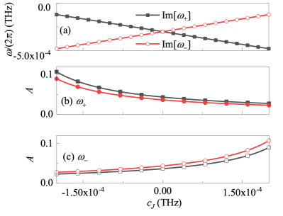
Figure 2: (a) $c_{\rm J}$ dependence of the imaginary parts of eigen frequencies $\omega_{\rm\pm}$ at $k_{\rm y}=0$. (b-c) Excited by $\mbox{\boldmath$\mathrm{\omega}$}_{\rm H}=(0,h_{\rm y},h_{\rm z})e^{(ik_{\rm y}y-i\omega t)}$ with $h_{\rm y}=3\times 10^{-4}$ THz, $h_{\rm z}=3i\times 10^{-4}$ THz and $k_{\rm y}=0$, $c_{\rm J}$ dependence of excited oscillation amplitude for (b) $\omega={\rm Re}[\omega_{\rm+}]$ and (c) $\omega={\rm Re}[\omega_{\rm-}]$. Solid squares and open circles are respectively the amplitudes of the sublattice magnetization $\mbox{\boldmath$\mathrm{m}$}_{\rm 1}$ and $\mbox{\boldmath$\mathrm{m}$}_{\rm 2}$.

The STT also affects the magnon excitation efficiency. Using polarized microwave field $\mbox{\boldmath$\mathrm{\omega}$}_{\rm H}=(0,h_{\rm y},h_{\rm z})e^{(ik_{\rm y}y-i\omega t)}$ ($h_{\rm y}=3\times 10^{-4}$ THz, $h_{\rm z}=3i\times 10^{-4}$ THz, $k_{\rm y}=0$, and $\omega={\rm Re}[\omega_{\rm\pm}]$) and Eq. (8), we calculate amplitudes of the excited magnetization oscillations, see Fig. 2. Apparently the positive (negative) $c_{\rm J}$ decreases (increases) the efficiency of exciting magnons of $\omega_{\rm+}$ mode. The effect is reversed for $\omega_{\rm-}$ mode. In view of the changes in the imaginary parts of eigenfrequencies (Fig. 2(a)), we conclude that the effectiveness of exciting magnon increases if the imaginary parts of $\omega_{\rm\pm}$ is decreased, i.e., the effective magnon damping $\alpha_{\rm{\rm eff}}$ is lowered.

Enhancement and annihilation of magnons due to the STT are asymmetric and nonlinear, and the increase of the magnon amplitude is much stronger. This finding is in line with the STT induced magnon enhancement/annihilation in FM, where the enhancement (annihilation) occurs when electron polarization is opposite (parallel) to the magnon polarization and decreases (increases) the magnon effective damping Wang et al. (2017, 2018).

V Thermal effect and spin pumping

From the Eq. (1) we infer that the thermal magnons are excited by the thermal random fields $\mbox{\boldmath$\mathrm{h}$}_{\rm m}$ and $\mbox{\boldmath$\mathrm{h}$}_{\rm n}$. By solving the dynamic equations, we obtain the dynamic magnetic susceptibility matrix $\hat{\chi}(\omega)$ , and $l_{\rm p}(\omega)=\sum_{\rm q}\chi_{\rm pq}h_{\rm q}(\omega)$ with $l_{\rm 1}=m_{\rm y}$, $l_{\rm 2}=m_{\rm z}$, $l_{\rm 3}=n_{\rm y}$, $l_{\rm 4}=n_{\rm z}$, $h_{\rm 1}=h_{\rm m,y}$, $h_{\rm 2}=h_{\rm m,z}$, $h_{\rm 3}=h_{\rm n,y}$ and $h_{\rm 4}=h_{\rm n,z}$):

$$\hat{\chi}=\left(\begin{matrix}\frac{c_{\rm-}}{l_{\rm+}}-\frac{c_{\rm+}}{l_{\rm-}}&\frac{ic_{\rm-}}{l_{\rm+}}+\frac{ic_{\rm+}}{l_{\rm-}}&\frac{\omega}{l_{\rm+}}-\frac{\omega}{l_{\rm-}}&\frac{i\omega}{l_{\rm+}}+\frac{i\omega}{l_{\rm-}}\\ -\frac{ic_{\rm-}}{l_{\rm+}}-\frac{ic_{\rm+}}{l_{\rm-}}&\frac{c_{\rm-}}{l_{\rm+}}-\frac{c_{\rm+}}{l_{\rm-}}&-\frac{i\omega}{l_{\rm+}}-\frac{i\omega}{l_{\rm-}}&\frac{\omega}{l_{\rm+}}-\frac{\omega}{l_{\rm-}}\\ \frac{\omega}{l_{\rm+}}-\frac{\omega}{l_{\rm-}}&\frac{i\omega}{l_{\rm+}}+\frac{i\omega}{l_{\rm-}}&\frac{d_{\rm-}}{l_{\rm+}}-\frac{d_{\rm+}}{l_{\rm-}}&\frac{id_{\rm-}}{l_{\rm+}}+\frac{id_{\rm+}}{l_{\rm-}}\\ -\frac{i\omega}{l_{\rm+}}-\frac{i\omega}{l_{\rm-}}&\frac{\omega}{l_{\rm+}}-\frac{\omega}{l_{\rm-}}&-\frac{id_{\rm-}}{l_{\rm+}}-\frac{id_{\rm+}}{l_{\rm-}}&\frac{d_{\rm-}}{l_{\rm+}}-\frac{d_{\rm+}}{l_{\rm-}}\end{matrix}\right),$$ (9)

where $c_{\rm\pm}:=-ic_{\rm J}\pm(\omega_{\rm ak}-i\alpha\omega)$, and $d_{\rm\pm}:=-ic_{\rm J}\pm(\omega_{\rm k}-i\alpha\omega)$.

By virtue of spin pumping, the magnetization dynamics in the AFM can pump into the neighboring metal layer the spin currentJohansen and Brataas (2017)

$$\mbox{\boldmath$\mathrm{I}$}_{\rm{\rm sp}}=\frac{\hbar g_{\rm r}}{2\pi}(\mbox{\boldmath$\mathrm{m}$}\times\partial_{\rm t}\mbox{\boldmath$\mathrm{m}$}+\mbox{\boldmath$\mathrm{n}$}\times\partial_{\rm t}\mbox{\boldmath$\mathrm{n}$}).$$ (10)

Here, $g_{\rm r}=G_{\rm r}h/e^{2}$ is the rescaled interface mixing conductance. In contrast to spin pumping current, the fluctuation spin current $\mbox{\boldmath$\mathrm{I}$}_{\rm{\rm fl}}=-\frac{2M_{\rm s}}{\gamma}(\mbox{\boldmath$\mathrm{m}$}\times\mbox{\boldmath$\mathrm{h}$}^{\prime}_{\rm m}+\mbox{\boldmath$\mathrm{n}$}\times\mbox{\boldmath$\mathrm{h}$}^{\prime}_{\rm n})$ flows back to the AFM Xiao et al. (2010). $\mbox{\boldmath$\mathrm{h}$}^{\prime}_{\rm m}$ and $\mbox{\boldmath$\mathrm{h}$}^{\prime}_{\rm n}$ satisfy the time correlation $\langle h^{\prime}_{\rm m,p}(\mbox{\boldmath$\mathrm{r}$},t)h^{\prime}_{\rm m,q}(\mbox{\boldmath$\mathrm{r}$}^{\prime},t^{\prime})\rangle=\langle h^{\prime}_{\rm n,p}(\mbox{\boldmath$\mathrm{r}$},t)h^{\prime}_{\rm n,q}(\mbox{\boldmath$\mathrm{r}$}^{\prime},t^{\prime})\rangle=\delta_{\rm pq}\delta(t-t^{\prime})\delta(\mbox{\boldmath$\mathrm{r}$}-\mbox{\boldmath$\mathrm{r}$}^{\prime})\frac{\alpha^{\prime}\gamma k_{\rm B}T}{\mu_{\rm 0}M_{\rm s}V}$, and $\alpha^{\prime}=\gamma\hbar g_{\rm r}/(4\pi M_{\rm s}V)$. The net spin current injected into the neighboring metal is $\mbox{\boldmath$\mathrm{I}$}_{\rm s}=\mbox{\boldmath$\mathrm{I}$}_{\rm{\rm sp}}+\mbox{\boldmath$\mathrm{I}$}_{\rm{\rm fl}}$ . Then, with the magnon dynamics described by Eq. (9), the time derivative of the correlation function for $\mbox{\boldmath$\mathrm{I}$}_{\rm{\rm sp}}$ within the macrospin model ($k_{\rm y}=0$) is

$$\langle\dot{l}_{\rm p}l_{\rm q}\rangle=\sigma^{2}_{\rm T}\int i\omega\sum_{\rm n}\chi_{\rm pn}(\omega)\chi_{\rm qn}(-\omega)\frac{d\omega}{2\pi}.$$ (11)

$p,q,n=1,2,3,4$. Using the contour integration method, we derive the finite $x$ component of the spin current $I_{\rm{\rm sp,x}}$ as

$$\langle I_{\rm{\rm sp,}x}\rangle=\frac{\hbar g_{\rm r}\sigma^{2}_{\rm T}c_{\rm J}(\omega_{\rm ak}+\omega_{\rm k})}{2\pi(c_{\rm J}^{2}-\alpha^{2}\omega_{\rm ak}\omega_{\rm k})}.$$ (12)

The two other components of the spin current vanish $\langle I_{\rm sp,y}\rangle=\langle I_{\rm sp,z}\rangle=0$. The above equation indicates that the spin pumping current’s polarization is parallel to the electron polarization and the equilibrium N${\rm\acute{e}}$el order vector. Without STT, two degenerate magnon modes are equally excited by thermal fluctuation, and the pumping current $\langle I_{\rm sp,x}\rangle=0$. Below the critical value $c_{\rm J}<\alpha\sqrt{\omega_{\rm A}\omega_{\rm k}}$ (above which the STT changes the stable state), positive $c_{\rm J}$ creates the negative $\langle I_{\rm sp,x}\rangle$. The reason is that positive $c_{\rm J}$ enhances the $\omega_{\rm-}$ mode polarized towards $-x$ (generating negative pumping current) but weakens the $\omega_{\rm+}$ mode polarized towards $+x$ (generating positive pumping current). The sign of $\langle I_{\rm{\rm sp,}x}\rangle$ changes with reversing the direction of the electric current (the sign of $c_{\rm J}$). The change of the magnon density induced by STT is nonlinear (see Fig. 2), and therefore the amplitude of $\langle I_{\rm sp,x}\rangle$ also changes nonlinearly with $c_{\rm J}$. The fluctuating spin current vanishes $\mbox{\boldmath$\mathrm{I}$}_{\rm{\rm fl}}=0$. Thus, the net current is equal to the spin pumping current $\langle I_{\rm s,x}\rangle=\langle I_{\rm sp,x}\rangle$. Numerical results calculated from Eq. (12) are shown in Fig. 3(a) and support the analytical findings.

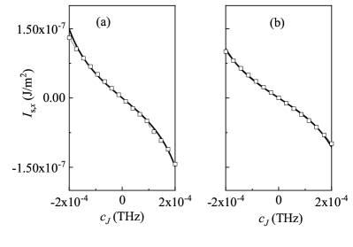
Figure 3: $c_{\rm J}$ dependence of net current $\langle I_{\rm s,x}\rangle$ at $T=30$ K for (a) macrospin and (b) 1D models. Analytical (solid lines) and numerically simulated (open dots) results are shown.

We extended the results obtained for the single macrospin model to the spatially inhomogeneous dynamical modes (i.e., excited finite wavevector $\mathrm{k}$), and obtain the time derivative of the correlation function $\mbox{\boldmath$\mathrm{I}$}_{\rm{\rm sp}}$

$$\langle\dot{l}_{\rm p}l_{\rm q}\rangle=\sigma^{2}_{\rm T}S_{\rm\zeta}\int\frac{d^{\zeta}\mbox{\boldmath$\mathrm{k}$}}{(2\pi)^{\zeta}}\int i\omega\sum_{\rm n}\chi_{\rm pn}(\omega,\mbox{\boldmath$\mathrm{k}$})\chi_{\rm qn}(-\omega,-\mbox{\boldmath$\mathrm{k}$})\frac{d\omega}{2\pi}.$$ (13)

Here, $\zeta=1$ is for the one-dimensional (1D) model ($\mbox{\boldmath$\mathrm{k}$}=k_{\rm y}\mbox{\boldmath$\mathrm{e}$}_{\rm y}$ and $S_{\rm 1}$ is the sample length along $y$). For the two-dimensional (2D) model $\zeta=2$, ($\mbox{\boldmath$\mathrm{k}$}=k_{\rm x}\mbox{\boldmath$\mathrm{e}$}_{\rm x}+k_{\rm y}\mbox{\boldmath$\mathrm{e}$}_{\rm y}$ and $S_{\rm 2}=S_{\rm xy}$ is the area of the sample plane).

Due to the limited size of discrete unit cell, the value of magnon wavevector can not be too large. We integrate Eq. (13) in the finite range of $-k_{\rm c}<k_{\rm x,y}<k_{\rm c}$ with $k_{\rm c}=\pi/l_{\rm y}$, where $l_{\rm y}$ is the unit cell size. For a 1D model, we infer

$$\langle I_{\rm{\rm sp,}x}\rangle=\hbar g_{\rm r}\sigma_{\rm T}^{2}l_{\rm y}c_{\rm J}(\omega_{\rm A}+\omega_{\rm E})\times$$ (14)

$$\frac{(\omega_{\rm j+}{\rm atan}(\frac{\alpha ak_{\rm c}\sqrt{\omega_{\rm E}}}{2\omega_{\rm j-}})-\omega_{\rm j-}{\rm atan}(\frac{\alpha ak_{\rm c}\sqrt{\omega_{\rm E}}}{2\omega_{\rm j+}})))}{2\pi^{2}\omega_{\rm j+}\omega_{\rm j-}\sqrt{\alpha^{2}(\omega_{\rm A}+\omega_{\rm E})^{2}-c_{\rm J}^{2}}},$$

with

$$\omega_{\rm j\pm}=\sqrt{\alpha(\pm\sqrt{\alpha^{2}(\omega_{\rm A}+\omega_{\rm E})^{2}-c_{\rm J}^{2}}-\alpha\omega_{\rm E})}.$$ (15)

If STT is applied $c_{\rm J}\neq 0$, the variation of $\langle I_{\rm{\rm sp,}x}\rangle$ for 1D model is similar to that for macrospin, including the aspects of sign and nonlinearity, as confirmed by numerical calculations in Fig. 3(b).

To quantify the effectiveness of the above conversion process, we compare the difference between the injected electronic spin current and output magnonic pumping current. Here, via $J_{\rm s}^{x}=-\frac{2c_{\rm J}}{\mu_{\rm 0}d_{\rm AF}M_{\rm s}}$, the $x$ component of electronic spin current density $J_{\rm s}^{x}$ is directly determined from the amplitude $c_{\rm J}$ of STT Chen et al. (2013). With the above parameters, we find $J_{\rm s}^{x}=-5.5\times 10^{-7}$ J/m² under $c_{\rm J}=2\times 10^{-4}$ THz; and in this case around 27 % electronic spin current is converted into the magnonic pumping current in Fig. 3.

To support the analytical results, we numerically solved for the LLG Eqs. (1). In the numerical simulation the spin pumping current’s value is determined from the expression Eq. (10). Under the same parameters adopted above, we compare the simulation results with the analytical calculations in Fig. 3, confirming the value of the analytical expressions. In addition, we consider the case with the electron spin polarization $\mbox{\boldmath$\mathrm{\mu}$}_{\rm s}^{N}=(0,1,0)$ being perpendicular to the equilibrium N${\rm\acute{e}}$el order vector $\mbox{\boldmath$\mathrm{n}$}_{\rm 0}$. Our calculations show that the STT does not affect the magnons in the AFM in this case, and therefore $\langle I_{\rm{\rm sp,}x}\rangle=0$. This conclusion is confirmed also by the numerical simulation.

VI Applying magnetic field along x

An applied magnetic field impacts the magnon polarization and leads to the nontrivial phenomena of electron-magnon spin conversion in the AFM /heavy heterostructure. Here, we mainly consider the case with the external magnetic field $\omega_{\rm Hx}$ applied along the easy-axis (x axis), for $\omega_{\rm Hx}<\sqrt{2\omega_{\rm E}\omega_{\rm A}}=1.7$ THz. In this range, the linear antiparallel structure ($\mbox{\boldmath$\mathrm{m}$}_{\rm 0}=(0,0,0)$ and $\mbox{\boldmath$\mathrm{n}$}_{\rm 0}=(1,0,0)$) is stable. In the same manner we obtain the eigenfrequencies $\omega_{\rm\pm}$:

$$\omega_{\rm\pm} =\pm\sqrt{F_{\rm\pm}}+\omega_{\rm ch}-\frac{i\alpha}{2}\omega_{\rm ck}^{+},$$ (16)

where

$$F_{\rm\pm}= \frac{1}{2\omega_{\rm ch}}(-4c_{\rm J}^{2}\omega_{\rm Hx}+\alpha^{3}c_{\rm J}[4\omega_{\rm Hx}^{2}+(\omega_{\rm ck}^{-})^{2}]$$ (17)

$$+\alpha^{2}\omega_{\rm Hx}[8c_{\rm J}^{2}-4\omega^{2}-(\omega_{\rm ck}^{-})^{2}]+4\omega_{\rm Hx}\omega_{\rm k}\omega_{\rm A}$$

$$-4ic_{\rm j}\omega_{\rm ch}\omega_{\rm ck}^{+}+4\alpha[c_{\rm J}^{3}-i\omega_{\rm Hx}\omega_{\rm ch}\omega_{\rm ck}^{+}$$

$$-c_{\rm J}(2\omega_{\rm Hx}^{2}+\omega_{\rm k}\omega_{\rm ak})]),$$

where $\omega_{\rm ch}=\omega_{\rm Hx}-\alpha c_{\rm J}$, and $\omega_{\rm ck}^{\pm}=\omega_{\rm k}\pm\omega_{\rm ak}$. For the parameters considered above, we calculate the magnon dispersion relations (Fig. 4(a-b)). The real parts of both modes $\omega_{\rm+}$ and $\omega_{\rm-}$ are shifted upward and the values of the corresponding imaginary parts are changed, steering the separation between ${\rm Im}[\omega_{\rm\pm}]$. These changes increase linearly with $\omega_{\rm Hx}$, as demonstrated in Fig. 4(c-d). STT affects mainly the imaginary parts, and ${\rm Im}[\omega_{\rm+}]$ (${\rm Im}[\omega_{\rm-}]$) is increased (decreased) by a positive $c_{\rm J}$ (cf. the calculated results in Fig. 4).

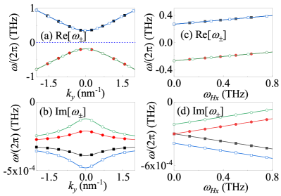
Figure 4: (a) Dispersion relations (i.e. real parts) and (b) imaginary parts of eigenfrequencies of $\omega_{\rm+}$ (squares) and $\omega_{\rm-}$ (circles) when $\omega_{\rm Hx}=0.1$ THz and $c_{\rm J}=0$ (solid dots) and $c_{\rm J}=0.0001$ THz (open dots). (c) Real and (d) imaginary parts of eigenfrequencies $\omega_{\rm\pm}$ as functions of $\omega_{\rm Hx}$ under $c_{\rm J}=0$ (solid dots) and $c_{\rm J}=0.0001$ THz (open dots).

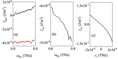
Figure 5: For a 1D model at the temperature $T=30$ K, (a) spin pumping spin current $\langle I_{\rm sp,x}\rangle$ (black squares for $c_{\rm J}=0$, red circles for $c_{\rm J}=1\times 10^{-4}$ THz) and (b) net spin current $\langle I_{\rm s,x}\rangle$ (when $c_{\rm J}=1\times 10^{-4}$ THz) as functions of magnetic field $\omega_{\rm Hx}$. (c) At $\omega_{\rm Hx}=0.7$ THz, $c_{\rm J}$ dependence of net current $\langle I_{\rm s,x}\rangle$.

The magnetic field induces a separation between the two degenerate modes $\omega_{\rm\pm}$, and at a finite temperature leads to a nonzero pumping current $I_{\rm sp,x}$ along the external magnetic field. The fluctuation spin current $\langle I_{\rm fl,x}\rangle$ is opposite to the pumping current $\langle I_{\rm sp,x}\rangle$, and the net current $\mbox{\boldmath$\mathrm{I}$}_{\rm s}$ is 0 if STT is not applied ($c_{\rm J}=0$). STT can further enhance one of two thermal magnon modes and weaken the other one, generating a nonzero $\mbox{\boldmath$\mathrm{I}$}_{\rm s}$, see Fig. 5(b). Surprisingly, the negative current $\langle I_{\rm s,x}\rangle$ induced by the positive $c_{\rm J}$ also increases with $\omega_{\rm Hx}$. When calculating the dependence of the net current $\langle I_{\rm s,x}\rangle$ on the $c_{\rm J}$ at finite $\omega_{\rm Hx}=0.7$ THz, we find that the positive $\omega_{\rm Hx}$ enhances the negative $\langle I_{\rm s,x}\rangle$, while it weakens the positive $\langle I_{\rm s,x}\rangle$, as compared to the case $\omega_{\rm Hx}=0$ (Fig. 3(b)). This effect leads to an asymmetric spin pumping in AFM induced by STT, and acts in favor of converting the electronic current into a magnonic spin current and vice versa.

VII External magnetic field along y

Under the influence of a strong magnetic field $\omega_{\rm Hx}$ applied along the x axis or $\omega_{\rm Hy}$ applied along y axis, the linear antiparallel orientation of AFM magnetization loses its stability and a spin-flop transition occurs. In this case, a nonzero net magnetization builds up along the magnetic field and increases with the amplitude of the magnetic field. The equilibrium N${\rm\acute{e}}$el order vector is perpendicular to the magnetic field. To explore the influences of the spin-flop on the net magnetization, we mainly study the case when $\omega_{\rm Hy}$ is applied along the y axis.

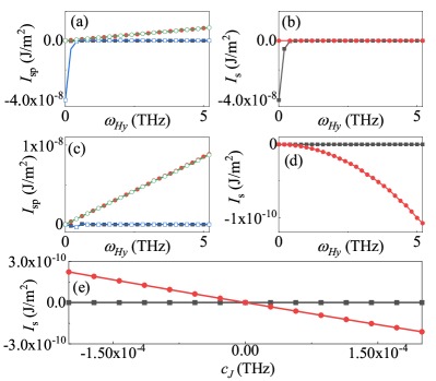
Figure 6: For 1D model at $T=30$ K, the $x$ component $\langle I_{\rm sp,x}\rangle$ (squares line) and the $y$ component $\langle I_{\rm sp,y}\rangle$ (circles line) of the spin pumping currents are shown as functions of the magnetic field $\omega_{\rm Hy}$, under $c_{\rm J}=0$ (solid dots) or $c_{\rm J}=1\times 10^{-4}$ THz (open dots) with (a) $\mbox{\boldmath$\mathrm{\mu}$}_{\rm s}^{N}=\mbox{\boldmath$\mathrm{x}$}$ and (c) $\mbox{\boldmath$\mathrm{\mu}$}_{\rm s}^{N}=\mbox{\boldmath$\mathrm{y}$}$. With $c_{\rm J}=1\times 10^{-4}$ THz and (b) $\mbox{\boldmath$\mathrm{\mu}$}_{\rm s}^{N}=\mbox{\boldmath$\mathrm{x}$}$ and (d) $\mbox{\boldmath$\mathrm{\mu}$}_{\rm s}^{N}=\mbox{\boldmath$\mathrm{y}$}$, the net spin currents $\langle I_{\rm s,x}\rangle$ (squares line) and $\langle I_{\rm s,y}\rangle$ (circles line) as functions of the magnetic field $\omega_{\rm Hy}$. (e) When $\omega_{\rm Hy}=5.2$ THz, $c_{\rm J}$ dependence of the net spin currents $\langle I_{\rm s,x}\rangle$ (squares line) and $\langle I_{\rm s,y}\rangle$ (circles line).

Applying positive $\omega_{\rm Hy}$ generates a net magnetization $\mbox{\boldmath$\mathrm{m}$}_{\rm 0}=(0,m_{\rm 0,y},0)$ with $m_{\rm 0,y}>0$. The thermal fluctuation of this net magnetization exerts a positive pumping current $\langle I_{\rm sp,y}\rangle$ along $y$, as shown by Fig. 6. This behavior is similar to the features of a thermal pumping current in FM Xiao et al. (2010). Along $x$ axis, the dynamics of opposite sublattice magnetizations are symmetric, and the pumping current in this case is zero $\langle I_{\rm sp,x}\rangle=0$ . Applying STT with $\mbox{\boldmath$\mathrm{\mu}$}_{\rm s}^{N}=(1,0,0)$ only affects $\langle I_{\rm sp,x}\rangle$, and a positive $c_{\rm J}$ drives a negative $\langle I_{\rm sp,x}\rangle$ and hence a negative net current $\langle I_{\rm s,x}\rangle$ (see Fig. 6(a-b)). This effect is similar to the effect described above (Fig. 3). However, the increase in $\omega_{\rm Hy}$ strongly weakens this effect, and $\langle I_{\rm sp,x}\rangle$ and $\langle I_{\rm s,x}\rangle$ approaches 0 for larger $\omega_{\rm Hy}$. To understand this phenomenon, we also analyze the change in ${\rm Im}[\omega_{\rm\pm}]$ induced by STT. However, this effect is negligible for lager $\omega_{\rm Hy}$ (not shown).

Applying STT with polarization $\mbox{\boldmath$\mathrm{\mu}$}_{\rm s}^{N}=(0,1,0)$ impacts the dynamics of the net magnetization along y. It enhances/weakens the thermal fluctuation of the net magnetization and hence $\langle I_{\rm sp,y}\rangle$. As demonstrated in Fig. 6(c-d), the positive $c_{\rm J}$ decreases the $\langle I_{\rm sp,y}\rangle$, generating a negative $\langle I_{\rm s,y}\rangle$. The induced $\langle I_{\rm s,y}\rangle$ increases with the net magnetization $m_{\rm 0,y}$ and thus magnetic field $\omega_{\rm Hy}$.

After reversing the sign of $c_{\rm J}$, the current $\langle I_{\rm s,y}\rangle$ becomes positive (Fig. 6(e)). With further increasing of the amplitude of $c_{\rm J}$ (not shown), we observe a nonlinear variation in $\langle I_{\rm s,y}\rangle$, where the negative $\langle I_{\rm s,y}\rangle$ can be larger than the positive $\langle I_{\rm s,y}\rangle$ under the same $|c_{\rm J}|$. This nonlinear and asymmetric variation in the net magnetization fluctuation resembles the effect in FM Wang et al. (2017). Noteworthy, as compared with the case in absence of the magnetic field and $\mbox{\boldmath$\mathrm{\mu}$}_{\rm s}^{N}\parallel\mbox{\boldmath$\mathrm{n}$}_{\rm 0}$, the current $\langle I_{\rm s,y}\rangle$ is much smaller (cf. Fig. 3), even when the magnetic field is sufficiently strong ($\omega_{\rm Hy}=5.2$ THz). Based on this observation we conclude, that when a finite net magnetization builds up along the external magnetic field, the induced spin pumping current is smaller than in the case of N${\rm\acute{e}}$el order vector.

VIII Conclusion

We studied the electron-magnon spin conversion process in a HM/AFM/HM heterostructure. A charge current in the metallic layer drives a spin dynamics in the AFM via spin transfer torques (STT) effects. Two degenerate AFM magnon modes with opposite polarization are involved. Depending on the electron polarization, STT enhances one of two modes and suppresses the other. At finite temperatures, the creation/annihilation of the two magnon modes in AFM by the STT leads to a net spin pumping current. This current increases nonlinearly with the electric current density in the HM layer. An external magnetic field can control the conversion process, which is shown to be quite efficient and potentially useful for designing antiferromagnetic-based spintronic devices.

IX ACKNOWLEDGMENT

This work was supported by the National Natural Science Foundation of China (No. 11674400, 11374373, 11704415), DFG through SFB 762 and SFB TRR227, and the Natural Science Foundation of Hunan Province of China (No. 2018JJ3629 and 2020JJ4104).

References

- Žutić et al. (2004) I. Žutić, J. Fabian, and S. Das Sarma, Rev. Mod. Phys. 76, 323 (2004).
- Chumak et al. (2015) A. V. Chumak, V. I. Vasyuchka, A. A. Serga, and B. Hillebrands, Nat. Phys. 11, 453 (2015).
- Wolf et al. (2001) S. A. Wolf, D. D. Awschalom, R. A. Buhrman, J. M. Daughton, S. von Molnár, M. L. Roukes, A. Y. Chtchelkanova, and D. M. Treger, Science 294, 1488 (2001).
- Ohno (2010) H. Ohno, Nat. Mater. 9, 952 (2010).
- Sinova et al. (2015) J. Sinova, S. O. Valenzuela, J. Wunderlich, C. H. Back, and T. Jungwirth, Rev. Mod. Phys. 87, 1213 (2015).
- Heinrich et al. (2011) B. Heinrich, C. Burrowes, E. Montoya, B. Kardasz, E. Girt, Y.-Y. Song, Y. Sun, and M. Wu, Phys. Rev. Lett. 107, 066604 (2011).
- Hirsch (1999) J. E. Hirsch, Phys. Rev. Lett. 83, 1834 (1999).
- Valenzuela and Tinkham (2006) S. O. Valenzuela and M. Tinkham, Nature 442, 176 (2006).
- Kato et al. (2004) Y. K. Kato, R. C. Myers, A. C. Gossard, and D. D. Awschalom, Science 306, 1910 (2004).
- Tserkovnyak et al. (2005) Y. Tserkovnyak, A. Brataas, G. E. W. Bauer, and B. I. Halperin, Rev. Mod. Phys. 77, 1375 (2005).
- Saitoh et al. (2006) E. Saitoh, M. Ueda, H. Miyajima, and G. Tatara, Appl. Phys. Lett. 88, 182509 (2006).
- Sandweg et al. (2011) C. W. Sandweg, Y. Kajiwara, A. V. Chumak, A. A. Serga, V. I. Vasyuchka, M. B. Jungfleisch, E. Saitoh, and B. Hillebrands, Phys. Rev. Lett. 106, 216601 (2011).
- Ando et al. (2011) K. Ando, S. Takahashi, J. Ieda, Y. Kajiwara, H. Nakayama, T. Yoshino, K. Harii, Y. Fujikawa, M. Matsuo, S. Maekawa, and E. Saitoh, J. Appl. Phys. 109, 103913 (2011).
- Uchida et al. (2010) K. Uchida, J. Xiao, H. Adachi, J. Ohe, S. Takahashi, J. Ieda, T. Ota, Y. Kajiwara, H. Umezawa, H. Kawai, G. E. W. Bauer, S. Maekawa, and E. Saitoh, Nat. Mater. 9, 894 (2010).
- Chumak et al. (2012) A. V. Chumak, A. A. Serga, M. B. Jungfleisch, R. Neb, D. A. Bozhko, V. S. Tiberkevich, and B. Hillebrands, Appl. Phys. Lett. 100, 082405 (2012).
- Kajiwara et al. (2010) Y. Kajiwara, K. Harii, S. Takahashi, J. Ohe, K. Uchida, M. Mizuguchi, H. Umezawa, H. Kawai, K. Ando, K. Takanashi, S. Maekawa, and E. Saitoh, Nature 464, 262 (2010).
- Wang et al. (2017) X.-g. Wang, Z.-x. Li, Z.-w. Zhou, Y.-z. Nie, Q.-l. Xia, Z.-m. Zeng, L. Chotorlishvili, J. Berakdar, and G.-h. Guo, Phys. Rev. B 95, 020414 (2017).
- Chotorlishvili et al. (2019) L. Chotorlishvili, Z. Toklikishvili, X.-G. Wang, V. K. Dugaev, J. Barnaś, and J. Berakdar, Phys. Rev. B 99, 024410 (2019).
- Wang et al. (2012) X.-g. Wang, G.-h. Guo, Y.-z. Nie, G.-f. Zhang, and Z.-x. Li, Phys. Rev. B 86, 054445 (2012).
- Jungwirth et al. (2016) T. Jungwirth, X. Marti, P. Wadley, and J. Wunderlich, Nat. Nanotechnol. 11, 231 (2016).
- Gomonay and Loktev (2014) E. V. Gomonay and V. M. Loktev, Low Temp. Phys. 40, 17 (2014).
- Baltz et al. (2018) V. Baltz, A. Manchon, M. Tsoi, T. Moriyama, T. Ono, and Y. Tserkovnyak, Rev. Mod. Phys. 90, 015005 (2018).
- Gomonay et al. (2018) O. Gomonay, V. Baltz, A. Brataas, and Y. Tserkovnyak, Nat. Phys. 14, 213 (2018).
- Jungfleisch et al. (2018) M. B. Jungfleisch, W. Zhang, and A. Hoffmann, Phys. Lett. A 382, 865 (2018).
- Park et al. (2011) B. G. Park, J. Wunderlich, X. Martí, V. Holý, Y. Kurosaki, M. Yamada, H. Yamamoto, A. Nishide, J. Hayakawa, H. Takahashi, A. B. Shick, and T. Jungwirth, Nature Materials 10, 347 (2011).
- Rezende et al. (2016a) S. M. Rezende, R. L. Rodríguez-Suárez, and A. Azevedo, Phys. Rev. B 93, 014425 (2016a).
- Rezende et al. (2016b) S. M. Rezende, R. L. Rodríguez-Suárez, and A. Azevedo, Phys. Rev. B 93, 054412 (2016b).
- Wadley et al. (2016) P. Wadley, B. Howells, J. Železný, C. Andrews, V. Hills, R. P. Campion, V. Novák, K. Olejník, F. Maccherozzi, S. S. Dhesi, S. Y. Martin, T. Wagner, J. Wunderlich, F. Freimuth, Y. Mokrousov, J. Kuneš, J. S. Chauhan, M. J. Grzybowski, A. W. Rushforth, K. W. Edmonds, B. L. Gallagher, and T. Jungwirth, Science 351, 587 (2016).
- Wu et al. (2016) S. M. Wu, W. Zhang, A. KC, P. Borisov, J. E. Pearson, J. S. Jiang, D. Lederman, A. Hoffmann, and A. Bhattacharya, Phys. Rev. Lett. 116, 097204 (2016).
- Chen et al. (2018) X. Z. Chen, R. Zarzuela, J. Zhang, C. Song, X. F. Zhou, G. Y. Shi, F. Li, H. A. Zhou, W. J. Jiang, F. Pan, and Y. Tserkovnyak, Phys. Rev. Lett. 120, 207204 (2018).
- Wang et al. (2014) H. Wang, C. Du, P. C. Hammel, and F. Yang, Phys. Rev. Lett. 113, 097202 (2014).
- Lin et al. (2016) W. Lin, K. Chen, S. Zhang, and C. L. Chien, Phys. Rev. Lett. 116, 186601 (2016).
- Moriyama et al. (2015) T. Moriyama, S. Takei, M. Nagata, Y. Yoshimura, N. Matsuzaki, T. Terashima, Y. Tserkovnyak, and T. Ono, Appl. Phys. Lett. 106, 162406 (2015).
- Li et al. (2020) J. Li, C. B. Wilson, R. Cheng, M. Lohmann, M. Kavand, W. Yuan, M. Aldosary, N. Agladze, P. Wei, M. S. Sherwin, and J. Shi, Nature 578, 70 (2020).
- Vaidya et al. (2020) P. Vaidya, S. A. Morley, J. van Tol, Y. Liu, R. Cheng, A. Brataas, D. Lederman, and E. del Barco, Science 368, 160 (2020).
- Lebrun et al. (2018) R. Lebrun, A. Ross, S. A. Bender, A. Qaiumzadeh, L. Baldrati, J. Cramer, A. Brataas, R. A. Duine, and M. Kläui, Nature 561, 222 (2018).
- Dabrowski et al. (2020) M. Dabrowski, T. Nakano, D. M. Burn, A. Frisk, D. G. Newman, C. Klewe, Q. Li, M. Yang, P. Shafer, E. Arenholz, T. Hesjedal, G. van der Laan, Z. Q. Qiu, and R. J. Hicken, Phys. Rev. Lett. 124, 217201 (2020).
- Cheng et al. (2016) R. Cheng, D. Xiao, and A. Brataas, Phys. Rev. Lett. 116, 207603 (2016).
- Johansen and Brataas (2017) O. Johansen and A. Brataas, Phys. Rev. B 95, 220408 (2017).
- Chotorlishvili et al. (2015) L. Chotorlishvili, S. Etesami, J. Berakdar, R. Khomeriki, and J. Ren, Physical Review B 92, 134424 (2015).
- Johansen et al. (2018) O. Johansen, H. Skarsvåg, and A. Brataas, Phys. Rev. B 97, 054423 (2018).
- Chen et al. (2013) Y.-T. Chen, S. Takahashi, H. Nakayama, M. Althammer, S. T. B. Goennenwein, E. Saitoh, and G. E. W. Bauer, Phys. Rev. B 87, 144411 (2013).
- Wang et al. (2018) X.-g. Wang, Z.-w. Zhou, Y.-z. Nie, Q.-l. Xia, and G.-h. Guo, Phys. Rev. B 97, 094401 (2018).
- Xiao et al. (2010) J. Xiao, G. E. W. Bauer, K.-c. Uchida, E. Saitoh, and S. Maekawa, Phys. Rev. B 81, 214418 (2010).