Abstract
“Wisdom of crowds” refers to the phenomenon that the average opinion of a group of
individuals on a given question can be very close to the true answer.
It requires a large group diversity of opinions, but the collective error, the difference between the average opinion and the true value, has to be small.
We consider a stochastic opinion dynamics where individuals can change their opinion based on the opinions of others (social influence ), but to some degree also stick to their initial opinion (individual conviction ).
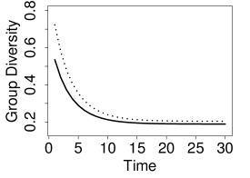
We then derive analytic expressions for the dynamics of the collective error and the group diversity.
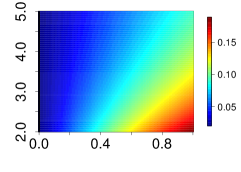
We analyze their long-term behavior to determine the impact of the two parameters and the initial opinion distribution on the wisdom of crowds.
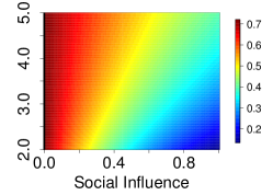
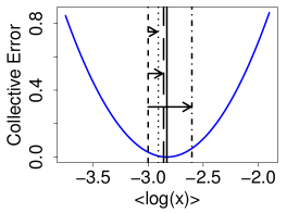
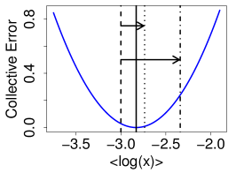
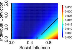
This allows us to quantify the ambiguous role of social influence: only if the initial collective error is large, it helps to improve the wisdom of crowds, but in most cases it deteriorates the outcome.
In these cases, individual conviction still improves the wisdom of crowds because it mitigates the impact of social influence.
[5]
Keywords: opinion dynamics, opinion distribution, collective effects, group decisions
[6]
 (b)
(b)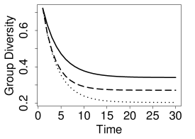
 (b)
(b)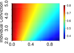
 (b)
(b)
 (c)
(c)