A least-squares Galerkin gradient recovery method for fully nonlinear elliptic equations

Abstract.

We propose a least squares Galerkin based gradient recovery to approximate Dirichlet problems for strong solutions of linear elliptic problems in nondivergence form and corresponding a priori and a posteriori error bounds. This approach is used to tackle fully nonlinear elliptic problems, e.g., Monge–Ampère, Hamilton–Jacobi–Bellman, using the smooth (vanilla) and the semismooth Newton linearization. We discuss numerical results, including adaptive methods based on the a posteriori error indicators.

1. Introduction

Let $\varOmega$ denote a bounded convex domain in $\mathbb{R}^{d}$, $d\in\mathbb{N}$ (typically $d=2,3$). Consider the Dirichlet problem of finding a function $u:\varOmega\to\mathbb{R}$ such that

(1) $$\mathcal{{F}}[x,u,\nabla{u},\operatorname{D}\!^{2}u]=0\text{ and }\left.u\right|_{\partial{\varOmega}}=r.$$

Here, $\nabla{u},\operatorname{D}\!^{2}u$ denote the gradient and the Hessian of $u$ and $\mathcal{{F}}:\varOmega\times\mathbb{R}\times\mathbb{R}^{d}\times\mathbb{R}^{d\times d}\to\mathbb{R}$ is assumed to be elliptic and Newton differentiable which is defined by Definition 3.1.

While viscosity solutions are possible, in a natural way, for this type of equations, we here focus on smoother solutions. Namely, we look at the numerical approximations of $u$ in $\operatorname{H}^{2}(\varOmega)$ satisfying (1), termed strong solution. We follow a series of papers on the matter (Smears and Süli, 2016; Feng and Jensen, 2017; Gallistl and Süli, 2019), but with a focus on the different and somewhat more flexible numerical methodology of least squares gradient recovery Galerkin finite element method to discretize the linear equations in nondivergence form that ensue from linearizing (1) using semismooth Newton method. We only state the results here, respectively referring for the details of §2 and §3 to Lakkis and Mousavi (2019) and Lakkis and Mousavi (2020). We look at some numerical examples, outlining an adaptive algorithm based on a posteriori error estimates for the linear elliptic equations in nondivergence form with Cordes coefficients.

2. A least-squares Galerkin approach to gradient recovery for linear equations in nondivergence form

We outline the proposed numerical method of the strong solution of the linear second order equation in nondivergence form; the details, including the proofs of all stated results can be found in Lakkis and Mousavi (2019). To prevent difficulties arising from numerically working in $\operatorname{H}^{2}(\varOmega)$ space, we consider an equivalent problem with solution in a $\operatorname{H}^{1}$-regularity space. For this we minimize a cost (least-squares) functional associated to the main problem. We prove that the equivalent problem is well posed using a coercivity argument, deducing thus the same result for the discrete counterpart. By setting Galerkin finite element spaces within $\operatorname{H}^{1}(\varOmega)$, we provide a priori and a posteriori error bounds.

Dropping the index $\alpha$ from the $\mathcal{{L}}^{\alpha}$ in (LABEL:eq:def:general-nonlinear-HJB-operator), we consider the following linear second order elliptic equations in nondivergence form of finding $u\in\operatorname{H}^{2}(\varOmega)$ such that

(2) $$\mathcal{{L}}u:=\boldsymbol{{A}}:\operatorname{D}\!^{2}u+\boldsymbol{b}{}^{\intercal}\nabla u-cu=f\text{ and }\left.u\right|_{\partial\varOmega}=0$$

where the coefficients $\boldsymbol{{A}}\in\operatorname{L}_{\infty}(\varOmega;\operatorname{Sym}{(\mathbb{R}^{d})})$, with $\operatorname{Sym}(X)=:\text{{symmetric\leavevmode\nobreak\ operators on} X}$, is uniformly elliptic, $\boldsymbol{b}\in\operatorname{L}_{\infty}(\varOmega;\mathbb{R}^{d})$ and $c\in\operatorname{L}_{\infty}(\varOmega)$, $c\geqslant 0$ satisfy exactly one of the following two Cordes conditions for some $\varepsilon\in\left(0,1\right)$

(3) $$\boldsymbol{b}\neq\boldsymbol{0}\text{ or }c\neq 0\>\Rightarrow\>\dfrac{\left|\boldsymbol{{A}}\right|^{2}+\nicefrac{{\left|\boldsymbol{b}\right|^{2}}}{{2\lambda}}+(\nicefrac{{c}}{{\lambda}})^{2}}{(\operatorname{tra}\boldsymbol{{A}}+\nicefrac{{c}}{{\lambda}})^{2}}\leqslant\dfrac{1}{d+\varepsilon}\text{${\ }\operatorname{a.e.}$in }\varOmega\text{ for some }\lambda>0,,$$

(4) $$\boldsymbol{b}\equiv\boldsymbol{0}\text{ and }c\equiv 0\>\Rightarrow\>\dfrac{\left|\boldsymbol{{A}}\right|^{2}}{(\operatorname{tra}\boldsymbol{{A}})^{2}}\leqslant\dfrac{1}{d-1+\varepsilon}\text{${\ }\operatorname{a.e.}$in }\varOmega,$$

where $\left|\boldsymbol{{X}}\right|=\big{(}\operatorname{tra}\boldsymbol{{X}}{}^{\intercal}\boldsymbol{{X}}\big{)}^{\nicefrac{{1}}{{2}}}$. The right-hand side $f$ is a generic element of $\operatorname{L}_{2}(\varOmega)$. We consider the right-hand side $r$ in (1) to be $0$ for simplicity (although the developments can be extended to $\left.r\right|_{\partial{\varOmega}}$ being the trace of a function $r\in\operatorname{H}^{2}(\varOmega)$.

Problem (2) is well posed under these assumptions as shown by Smears and Süli (2014). In numerical approximating solutions, dealing with more regular than $\operatorname{H}^{1}(\varOmega)$ spaces leads to complicated computations. To avoid this difficulty, we intend to consider an alternative equivalent problem with $\operatorname{H}^{1}(\varOmega)$ solution.

We denote the outer normal to $\varOmega$ at $\boldsymbol{x}\in\partial\varOmega$ by $\boldsymbol{n}_{\varOmega}(\boldsymbol{x})$, which we assume defined for $\mathcal{{S}}$-almost every $\boldsymbol{x}\in\partial\varOmega$ ($\mathcal{{S}}$ being the $(d-1)$-dimensional “surface” measure) and recall the tangential trace of $\boldsymbol{\psi}\in\operatorname{H}^{1}(\varOmega;\mathbb{R}^{d})$ is expressed (or defined) by

(5) $$\left({\boldsymbol{I}-\boldsymbol{n}_{\varOmega}\boldsymbol{n}_{\varOmega}{}^{\intercal}}\right)\left.\boldsymbol{\psi}\right|_{\partial{\varOmega}}.$$

Define the following function spaces

(6) $$\mathscr{{W}}:=\left\{\boldsymbol{\psi}\in\operatorname{H}^{1}(\varOmega;\mathbb{R}^{d}):\left({\boldsymbol{I}-\boldsymbol{n}_{\varOmega}\boldsymbol{n}_{\varOmega}{}^{\intercal}}\right)\left.\boldsymbol{\psi}\right|_{\partial\varOmega}=0\right\},$$

(7) $$\mathscr{{Y}}:=\operatorname{H}^{1}(\varOmega)\times\operatorname{H}^{1}\left({\varOmega;\mathbb{R}^{d}}\right)$$

(8) $$\mathscr{{V}}:=\operatorname{H}^{1}_{0}(\varOmega)\times\mathscr{{W}}\subseteq\mathscr{{Y}},$$

endowed with the $\operatorname{H}^{1}$-norm for $\mathscr{{W}}$ and the following norm for $\mathscr{{Y}}$ and $\mathscr{{V}}$,

(9) $$\left\|{(\varphi,\boldsymbol{\psi})}\right\|_{\mathscr{{Y}}}^{2}:=\left\|{\varphi}\right\|_{\operatorname{H}^{1}(\varOmega)}^{2}+\left\|{\boldsymbol{\psi}}\right\|_{\operatorname{H}^{1}(\varOmega)}^{2}\text{ for each }(\varphi,\boldsymbol{\psi})\in\mathscr{{Y}}\supseteq\mathscr{{V}}.$$

We denote by $\left\langle{\varphi,\psi}\right\rangle$ the $\operatorname{L}_{2}(D;V)$ inner product with respect to the Lebesgue or surface measure on $D$. For a fixed $\theta\in\left[0,1\right]$ we introduce the linear operator $\mathcal{{M}}_{\theta}:\mathscr{{Y}}\to\operatorname{L}_{2}(\varOmega)$

(10) $$\begin{gathered}(\varphi,\boldsymbol{\psi})\mapsto\boldsymbol{{A}}:\operatorname{D}\!\boldsymbol{\psi}+\boldsymbol{b}{}^{\intercal}(\theta\boldsymbol{\psi}+(1-\theta)\nabla\varphi)-c\varphi=:\mathcal{{M}}_{\theta}(\varphi,\boldsymbol{\psi}).\end{gathered}$$

The parameter $\theta$ is at the user’s disposal, but the most useful values are $0$, $\nicefrac{{1}}{{2}}$ and $1$. We introduce the following quadratic functional of $(\varphi,\boldsymbol{\psi})\in\mathscr{{V}}$

(11) $$\begin{gathered}E_{\theta}(\varphi,\boldsymbol{\psi}):=\left\|{\nabla\varphi-\boldsymbol{\psi}}\right\|_{\operatorname{L}_{2}(\varOmega)}^{2}+\left\|{\nabla\!\times\!\boldsymbol{\psi}}\right\|_{\operatorname{L}_{2}(\varOmega)}^{2}+\left\|{\mathcal{{M}}_{\theta}(\varphi,\boldsymbol{\psi})-f}\right\|_{\operatorname{L}_{2}(\varOmega)}^{2}\end{gathered}$$

where $\nabla\!\times\!\boldsymbol{\psi}$ denotes curl (rotation) of $\boldsymbol{\psi}$, and then consider the convex minimization problem of finding

(12) $$(u,\boldsymbol{g})=\underset{\begin{subarray}{c}\left({\varphi,\boldsymbol{\psi}}\right)\in\mathscr{{V}}\end{subarray}}{\operatorname{argmin}}E_{\theta}(\varphi,\boldsymbol{\psi}).$$

2.1. Remark (Equivalent problems)

The problem of finding strong solution to (2) and convex minimization problem (12) are equivalent and in (12), $\boldsymbol{g}=\nabla u$ holds. Thus, in the rest of the paper, $\boldsymbol{g}$ is equal to $\nabla u$.

The Euler–Lagrange equation of the minimization problem (12) consists in finding ${(u,\boldsymbol{g})\in\mathscr{{V}}}$ such that

(13) $$\left\langle{\nabla u-\boldsymbol{g},\nabla\varphi-\boldsymbol{\psi}}\right\rangle+\left\langle{\nabla\!\times\!\boldsymbol{g},\nabla\!\times\!\boldsymbol{\psi}}\right\rangle+\left\langle{\mathcal{{M}}_{\theta}(u,\boldsymbol{g}),\mathcal{{M}}_{\theta}(\varphi,\boldsymbol{\psi})}\right\rangle\\ =\left\langle{f,\mathcal{{M}}_{\theta}(\varphi,\boldsymbol{\psi})}\right\rangle\leavevmode\nobreak\ \text{ for each }(\varphi,\boldsymbol{\psi})\in\mathscr{{V}}.$$

We introduce the symmetric bilinear form ${a_{\theta}:\mathscr{{Y}}^{2}\to\mathbb{R}}$ via

(14) $$a_{\theta}(\varphi,\boldsymbol{\psi};\varphi^{\prime},\boldsymbol{\psi}^{\prime}):=\left\langle{\nabla\varphi-\boldsymbol{\psi},\nabla\varphi^{\prime}-\boldsymbol{\psi}^{\prime}}\right\rangle+\left\langle{\nabla\!\times\!\boldsymbol{\psi},\nabla\!\times\!\boldsymbol{\psi}^{\prime}}\right\rangle+\left\langle{\mathcal{{M}}_{\theta}(\varphi,\boldsymbol{\psi}),\mathcal{{M}}_{\theta}(\varphi^{\prime},\boldsymbol{\psi}^{\prime})}\right\rangle.$$

2.2. Theorem (Coercivity and continuity)

Let $\varOmega$ be a bounded convex open subset of $\mathbb{R}^{d}$ and the uniformly bounded coefficients $\boldsymbol{{A}},\boldsymbol{b},c$ satisfy either (3) with $\lambda>0$ or (4) with $\boldsymbol{b}\equiv\boldsymbol{0}$ and $c\equiv 0$. Then $a_{\theta}$ on $\mathscr{{V}}$ is coercive and continuous, there exist $C_{\textup{\ref{ineq:coercivity}{{}}}},C_{\textup{\ref{ineq:continuity}{{}}}}>0$ such that

(15) $$a_{\theta}\left({\varphi,\boldsymbol{\psi}\,;\,\varphi,\boldsymbol{\psi}}\right)\geqslant C_{\textup{\ref{ineq:coercivity}{{}}}}\left\|{(\varphi,\boldsymbol{\psi})}\right\|_{\mathscr{{Y}}}^{2}\text{ for each }(\varphi,\boldsymbol{\psi})\in\mathscr{{V}},$$

(16) $$\begin{aligned} a_{\theta}\left({\varphi,\boldsymbol{\psi}\,;\,\varphi^{\prime},\boldsymbol{\psi}^{\prime}}\right)\leqslant C_{\textup{\ref{ineq:continuity}{{}}}}\left\|{(\varphi,\boldsymbol{\psi})}\right\|_{\mathscr{{Y}}}\left\|{(\varphi^{\prime},\boldsymbol{\psi}^{\prime})}\right\|_{\mathscr{{Y}}}\text{ for each }(\varphi,\boldsymbol{\psi}),(\varphi^{\prime},\boldsymbol{\psi}^{\prime})\in\mathscr{{V}}.\end{aligned}$$

Theorem 2.2 ensures the well-posedness of the problem (13) trough the Lax-Milgram setting.

2.3. Definition of A least squares finite element method

Let $\mathfrak{T}$ be a collection of conforming shape-regular triangulations on $\varOmega$ which also known as meshes. If the domain, $\varOmega$, is a polyhedral then it coincides with the interior area of the mesh. Otherwise, if the domain includes curved boundary, the coincidence is lost. Hence this leads to have simplices with curved sides and isoparametric elements. For each element $K\in\mathcal{T}\in\mathfrak{T}$, denote $h_{K}:=\operatorname{diam}{K}$, and $h:=h_{\mathcal{T}}:=\max_{{K}\in\mathcal{T}}h_{K}$. Now, consider the following Galerkin finite element spaces

(17) $$\mathbb{U}{}:=\mathbb{P}^{k}\left({\mathcal{T}}\right)\cap\operatorname{H}^{1}_{0}(\varOmega),\quad\mathbb{G}{}:=\mathbb{P}^{k}(\mathcal{T};\mathbb{R}^{d})\cap\mathscr{{W}}\subseteq\operatorname{H}^{1}(\varOmega;\mathbb{R}^{d}).$$

Corresponding to these spaces, the discrete problem corresponding to (13) turns to finding $(\mathsf{u}_{\mathbb{U}{}},\boldsymbol{\mathsf{g}}{{}_{\mathbb{G}{}}})\in\mathbb{U}{}\times\mathbb{G}{}$ such that

(18) $$a_{\theta}(\mathsf{u}_{\mathbb{U}{}},\boldsymbol{\mathsf{g}}{{}_{\mathbb{G}{}}};\varphi,\boldsymbol{\psi})=\left\langle{f,\mathcal{{M}}_{\theta}(\varphi,\boldsymbol{\psi})}\right\rangle\text{ for each }(\varphi,\boldsymbol{\psi})\in\mathbb{U}{}\times\mathbb{G}{}.$$

The coercivity is inherited to subspaces, therefore the solution of discrete problem (18) is also well-posed. The discrete problem (18) leads to an approximate solution satisfying the following error estimate theorems.

2.4. Remark (implementing the boundary conditions)

Since imposing zero-tangential trace condition to the finite element spaces is not trivial. In the implementation we used in §4 we replace in (18) the space $\mathbb{G}{}:=\mathbb{P}^{k}\left({\mathcal{T};\mathbb{R}^{d}}\right)\cap\mathscr{{W}}\subseteq\operatorname{H}^{1}(\varOmega;\mathbb{R}^{d})$ with the larger space $\tilde{\mathbb{G}{}}:=\mathbb{P}^{k}\left({\mathcal{T};\mathbb{R}^{d}}\right)\cap\operatorname{H}^{1}(\varOmega;\mathbb{R}^{d})$.

2.5. Theorem (a priori error estimate)

Let $\mathcal{T}\in\mathfrak{T}$ be a mesh on the polyhedral domain $\varOmega\subseteq\mathbb{R}^{d}$. Moreover assume that the strong solution $u$ of (2) satisfies $u\in\operatorname{H}^{\beta+2}(\varOmega)$, for some real $\beta>0$. Let $(\mathsf{u}_{\mathbb{U}{}},\boldsymbol{\mathsf{g}}{{}_{\mathbb{G}{}}})\in\mathbb{U}{}\times\mathbb{G}{}$ be the finite element solution of (18) on the mesh $\mathcal{T}$. Then for some $C_{\textup{\ref{eqn:convergence-rate}{{}}}}>0$, independent of $u$ and $h$ we have

(19) $$\left\|{(u,\nabla u)-(\mathsf{u}_{\mathbb{U}{}},\boldsymbol{\mathsf{g}}{{}_{\mathbb{G}{}}})}\right\|_{\mathscr{{Y}}}\leqslant C_{\textup{\ref{eqn:convergence-rate}{{}}}}h^{\min{\left\{{k,\beta}\right\}}}\left\|{u}\right\|_{\operatorname{H}^{k+2}(\varOmega)}.$$

2.6. Remark (curved domain)

In the case that $\varOmega$ has a curved boundary we use isoparametric finite element. A piecewise smooth domain guarantees an optimal rate error bound using isoparametric finite element similarly to Theorem 2.5 (Ciarlet, 2002).

2.7. Theorem (error-residual a posteriori estimates)

Let $(\mathsf{u}_{\mathbb{U}{}},\boldsymbol{\mathsf{g}}{{}_{\mathbb{G}{}}})$ is the unique solution of the discrete problem (18).

1. The following a posteriori residual upper bound holds

   $$\left\|{(u,\nabla u)-(\mathsf{u}_{\mathbb{U}{}},\boldsymbol{\mathsf{g}}{{}_{\mathbb{G}{}}})}\right\|_{\mathscr{{Y}}}^{2}\leqslant C_{\textup{\ref{ineq:coercivity}{{}}}}^{-1}$$

   $$\qquad\left({\left\|{\nabla\mathsf{u}_{\mathbb{U}{}}-\boldsymbol{\mathsf{g}}{{}_{\mathbb{G}{}}}}\right\|_{\operatorname{L}_{2}(\varOmega)}^{2}+\left\|{\nabla\!\times\!\boldsymbol{\mathsf{g}}{{}_{\mathbb{G}{}}}}\right\|_{\operatorname{L}_{2}(\varOmega)}^{2}+\left\|{\mathcal{{M}}_{\theta}(\mathsf{u}_{\mathbb{U}{}},\boldsymbol{\mathsf{g}}{{}_{\mathbb{G}{}}})-f}\right\|_{\operatorname{L}_{2}(\varOmega)}^{2}}\right).$$

2. For any open subdomain $\omega\subseteq\Omega$ we have

   (20) $$\left\|{\nabla{\mathsf{u}_{\mathbb{U}{}}}-\boldsymbol{\mathsf{g}}{{}_{\mathbb{G}{}}}}\right\|_{\operatorname{L}_{2}(\omega)}^{2}+\left\|{\nabla\!\times\!\boldsymbol{\mathsf{g}}{{}_{\mathbb{G}{}}}}\right\|_{\operatorname{L}_{2}(\omega)}^{2}+\left\|{\mathcal{{M}}_{\theta}({\mathsf{u}_{\mathbb{U}{}}},{\boldsymbol{\mathsf{g}}{{}_{\mathbb{G}{}}}})-f}\right\|_{\operatorname{L}_{2}(\omega)}^{2}\\ \leqslant C_{\textup{\ref{ineq:continuity}{{,$\omega$}}}}\left({\left\|{u-\mathsf{u}_{\mathbb{U}{}}}\right\|_{\operatorname{H}^{1}{(\omega)}}^{2}+\left\|{\nabla u-\boldsymbol{\mathsf{g}}{{}_{\mathbb{G}{}}}}\right\|_{\operatorname{H}^{1}{(\omega)}}^{2}}\right),$$

   where $C_{\textup{\ref{ineq:continuity}{{,$\omega$}}}}$ is the continuity constant of $a_{\theta}$ restricted to $\omega\subseteq\Omega$.

3. Linearization of fully nonlinear problems

In this section, we present the Newton differentiability concept to operators, which can even include non-smooth operators. This concept is useful to extend the standard Newton linearization to the problems with non-smooth operator. We state the convergence analysis of a linearization method which is based on this concept. We then discuss linearization of two specific fully nonlinear PDEs, namely Monge–Ampère and Hamilton–Jacobi–Bellman equations that lead to a sequence of linear equations in nondivergence form.

3.1. Definition of Newton differentiable operator, Ito and Kunisch (2008)

Let $\mathscr{{X}}$ and $\mathscr{{Z}}$ be Banach spaces and let $\mathcal{U}$ be a non-empty open subset of $\mathscr{{X}}$. An operator $\mathcal{{F}}:\mathcal{U}\subset\mathscr{{X}}\to\mathscr{{Z}}$ is called Newton differentiable at $x\in\mathcal{U}$ if there exists a set-valued map with non-empty images $\operatorname{\mathfrak{D}}\mathcal{{F}}:\mathcal{U}\rightrightarrows\operatorname{Lin}\left({{\mathscr{{X}}}\to{\mathscr{{Z}}}}\right)$ (where the double arrow signifies values in the power set of the right-hand side) such that

(21) $$\lim_{\left\|{e}\right\|_{\mathscr{{X}}}\rightarrow 0}\dfrac{1}{\left\|{e}\right\|_{\mathscr{{X}}}}\sup_{\mathcal{{D}}\in\operatorname{\mathfrak{D}}\mathcal{{F}}[x]}\left\|{\mathcal{{F}}[x+e]-\mathcal{{F}}[x]-\mathcal{{D}}e}\right\|_{\mathscr{{Z}}}=0\text{ for each }x\in\mathcal{U}.$$

The nonlinear operator $\mathcal{{F}}$ is called Newton differentiable on $\mathcal{U}$ with Newton derivative $\operatorname{\mathfrak{D}}\mathcal{{F}}$ if $\mathcal{{F}}$ is Newton differentiable at $x$, for every $x\in\mathcal{U}$.

The set-valued map $\operatorname{\mathfrak{D}}\mathcal{{F}}[x]$ is single-valued at $x$ if and only if $\mathcal{{F}}$ is Fréchet differentiable and $\operatorname{\mathfrak{D}}\mathcal{{F}}[x]={\left\{{\operatorname{D}\!\mathcal{{F}}[x]}\right\}}$.

3.2. Theorem (Superlinear convergence)

Suppose that a nonlinear operator $\mathcal{{F}}$ is Newton differentiable in an open neighborhood $\mathcal{U}$ of $x^{\ast}$, solution of $\mathcal{{F}}[x]=0$. If for any $x\in U$, the all $D\in\operatorname{\mathfrak{D}}\mathcal{{F}}[x]$ are non-singular and $\left\|{D^{-1}}\right\|$ are bounded, then the Newton iteration

(22) $$x_{n+1}=x_{n}-D^{-1}_{n}\mathcal{{F}}[x_{n}],\quad D_{n}\in\operatorname{\mathfrak{D}}\mathcal{{F}}[x_{n}]$$

converges superlinearly to $x^{\ast}$ provided that $x_{0}$ is sufficiently close to $x^{\ast}$.

3.3. Definition of The Monge–Ampère equation

Let $\varOmega\subseteq\mathbb{R}^{2}$ be a bounded convex domain. Consider the Monge–Ampère (MA) equation with Dirichlet boundary condition

(23) $$\det\operatorname{D}\!^{2}u=f\text{ in }\varOmega,\left.u\right|_{\partial\varOmega}=0\text{ and }u\text{ is strictly convex in }\varOmega,$$

where $f\in\operatorname{L}_{2}(\varOmega)$, $f>0$ . Let $\mathscr{{K}}:=\left\{v\in\operatorname{H}^{2}(\varOmega)\cap\operatorname{H}^{1}_{0}(\varOmega):\;v\text{ is strictly convex}\right\}$ and define the operators $\operatorname{\mathscr{M}}:\mathscr{{K}}\to\operatorname{L}_{2}(\varOmega)$ by

(24) $$\operatorname{\mathscr{M}}[v]:=\det\operatorname{D}\!^{2}v-f$$

and $\operatorname{\mathfrak{D}}\operatorname{\mathscr{M}}:\mathscr{{K}}\to\operatorname{Lin}\left({{\operatorname{H}^{2}(\varOmega)\cap\operatorname{H}^{1}_{0}(\varOmega)}\to{\operatorname{L}_{2}(\varOmega)}}\right)$ by

(25) $$\operatorname{\mathfrak{D}}\operatorname{\mathscr{M}}[v]:=\operatorname{Cof}\operatorname{D}\!^{2}v:\operatorname{D}\!^{2}.$$

3.4. Theorem (superlinear convergence of iterative method to MA equation)

The operator $\operatorname{\mathscr{M}}$ is Fréchet differentiable and thus Newton differentiable. Moreover, if the initial guess $u_{0}\in\mathscr{{K}}$ is close to the exact solution $u\in\operatorname{H}^{2}(\varOmega)\cap\operatorname{H}^{1}_{0}(\varOmega)$ of (23), then the recursive problem

(26) $$\operatorname{Cof}\operatorname{D}\!^{2}u_{n}:\operatorname{D}\!^{2}u_{n+1}=f-\det\operatorname{D}\!^{2}u_{n}+\operatorname{Cof}\operatorname{D}\!^{2}u_{n}:\operatorname{D}\!^{2}u_{n}\leavevmode\nobreak\ \text{ in }\varOmega,\text{ and }\left.u_{n+1}\right|_{\partial\varOmega}=0$$

converges with superlinear rate to $u$.

3.5. Definition of Hamilton–Jacobi–Bellman equation

Let $\varOmega$ be a bounded convex domain in $\mathbb{R}^{d}$, $d\in\mathbb{N}$ (typically $d=2,3$). Consider the Hamilton–Jacobi–Bellman (HJB) equation with Dirichlet boundary condition

(27) $$\sup_{\alpha\in\mathcal{A}}\left(\boldsymbol{{A}}^{\alpha}:\operatorname{D}\!^{2}u+\boldsymbol{b}^{\alpha}{}^{\intercal}\nabla u-c^{\alpha}u-f^{\alpha}\right)=0\leavevmode\nobreak\ \text{ in }\varOmega\text{ and }\left.u\right|_{\partial\varOmega}=0$$

where $\mathcal{A}$ is a compact metric space, $\boldsymbol{{A}}\in\operatorname{L}_{\infty}(\varOmega;\operatorname{C}^{0}(\mathcal{A};\operatorname{Sym}{(\mathbb{R}^{d})}))$, $\boldsymbol{b}\in\operatorname{L}_{\infty}(\varOmega;\operatorname{C}^{0}(\mathcal{A};\mathbb{R}^{d}))$, $c\in\operatorname{L}_{\infty}(\varOmega;\operatorname{C}^{0}(\mathcal{A}))$ and $f\in\operatorname{L}_{2}(\varOmega;\operatorname{C}^{0}(\mathcal{A}))$. We suppose $\boldsymbol{{A}}^{\alpha}(\boldsymbol{x})$ is uniformly elliptic in both $\boldsymbol{x}$ and $\alpha$ and together with $\boldsymbol{b}^{\alpha},c^{\alpha}$ meets, for some $\epsilon\in\left(0,1\right)$ the Cordes condition (3), or (4) if $\boldsymbol{b}^{\alpha}\equiv\boldsymbol{0}$, $c^{\alpha}\equiv 0$, independent of $\alpha\in\mathcal{A}$. For each $\alpha\in\mathcal{A}$, define the linear operator

(28) $$\mathcal{{L}}^{\alpha}v:=\boldsymbol{{A}}^{\alpha}:\operatorname{D}\!^{2}v+\boldsymbol{b}^{\alpha}{}^{\intercal}\nabla v-c^{\alpha}v,$$

the following set of $\mathcal{A}$-index-valued maps:

(29) $$\mathcal{Q}:=\left\{q:\varOmega\rightarrow{\mathcal{A}}\left|\leavevmode\nobreak\ q\text{ is measurable}\right\}\right.,$$

and the set-valued map $\mathcal{N}$, for $v\in\operatorname{H}^{2}(\varOmega)\cap\operatorname{H}^{1}_{0}(\varOmega)$, such that

(30) $$\mathcal{N}[v]:=\left\{q\in\mathcal{Q}:\;q(\boldsymbol{x})\in\operatorname{Argmax}_{\alpha\in\mathcal{A}}\left({\left[{\mathcal{{L}}^{\alpha}v-f^{\alpha}}\right]\boldsymbol{x}}\right)\text{ for }{}\text{almost all }\boldsymbol{x}\text{ in }\varOmega\right\}.$$

Now, we define the HJB operator by

(31) $$\operatorname{\mathscr{B}}[v]:=\sup_{q\in\mathcal{Q}}\mathcal{{L}}^{q}v-f^{q},$$

and the set-valued map ${\operatorname{\mathfrak{D}}\operatorname{\mathscr{B}}:\operatorname{H}^{2}(\varOmega)\cap\operatorname{H}^{1}_{0}(\varOmega)\rightrightarrows\operatorname{Lin}\left({{\operatorname{H}^{2}(\varOmega)\cap\operatorname{H}^{1}_{0}(\varOmega)}\to{\operatorname{L}_{2}(\varOmega)}}\right)}$ by

(32) $$\operatorname{\mathfrak{D}}\operatorname{\mathscr{B}}[v]:=\left\{\mathcal{{L}}^{q}:=(\boldsymbol{{A}}^{q}:\operatorname{D}\!^{2}+\boldsymbol{b}^{q}{}^{\intercal}\nabla-c^{q})\left|\leavevmode\nobreak\ q\in\mathcal{N}[v]\right\}\right..$$

3.6. Theorem (superlinear convergence of iterative method to HJB equation)

The operator $\operatorname{\mathscr{B}}$ is Newton differentiable with Newton derivative $\operatorname{\mathfrak{D}}\operatorname{\mathscr{B}}$. Moreover, if the initial guess $u_{0}$ is close to the exact solution $u\in\operatorname{H}^{2}(\varOmega)\cap\operatorname{H}^{1}_{0}(\varOmega)$ of (27), the recursive problem

(33) $$\mathcal{{L}}^{q_{n}}u_{n+1}=f^{q_{n}}\text{ in }\varOmega,\text{ and }\left.u_{n+1}\right|_{\partial\varOmega}=0$$

where $q_{n}\in\mathcal{N}[u_{n}]$, converges with superlinear rate to $u$.

To follow (26) and (33), we need to approximate a linear problem in nondivergence form in each iteration, which we apply the method discussed in § 2. The convergence of the iterative methods (26) and (33) implies that the finite element approximation $(\mathsf{u}_{\mathbb{U}{}},\boldsymbol{\mathsf{g}}{{}_{\mathbb{G}{}}})\in\mathbb{U}{}\times\mathbb{G}{}$ achieved via the recursive problems also satisfies the error bound of Theorem 2.5 and 2.7.

3.7. Remark

The a posteriori residual bound of Theorem 2.7 can be used as an explicit error indicator to determine a locally refined mesh in the adaptive scheme.

4. Numerical experiments

We discuss two numerical tests one for each of Monge–Ampère via Newton and Hamilton–Jacobi–Bellman problems that demonstrate the robustness of our method to the fully nonlinear problems. For both test problems, the domain, $\varOmega$, is taken to be the unit disk in $\mathbb{R}^{2}$ with center at the origin. The criterion to stop the iteration is either $\left\|{(\mathsf{u}_{n+1},\boldsymbol{\mathsf{g}}{}_{n+1})-(\mathsf{u}_{n},\boldsymbol{\mathsf{g}}{}_{n})}\right\|_{\mathscr{{Y}}}<10^{-8}$ or maximum $8$ iterations. In implementation, we take the parameter $\theta$ of (18) equal to $0.5$. Both implementations were done by using FEniCS package.

In the first test problem, the known solution is considered smooth and we see that the numerical results which obtained on the uniform mesh confirm the convergence analysis of Theorem 2.5. In the second test problem, we choose the known solution near singular and test the performance of the adaptive scheme as mentioned in Remark 3.7. Through comparing the convergence rate by the adaptive with uniform refinement, we observe the efficiency of the adaptive scheme.

4.1. Problem (Monge–Ampère test)

Consider problem (23) and choose $f$ corresponding to the exact solution

(34) $$u(\boldsymbol{x})=-\sqrt{R^{2}-x_{1}^{2}-x_{2}^{2}}+\sqrt{R^{2}-1},\text{ for a fixed }R>1.$$

As suggested by Lakkis and Pryer (2013) the first iterate $\mathsf{u}_{0}$ is the discretization of $u_{0}$ satisfying

(35) $$\Delta u_{0}=2\sqrt{f}\leavevmode\nobreak\ \text{ in }\varOmega,\text{ and }\left.u_{0}\right|_{\partial\varOmega}=0$$

and then we track the recursive problem (26). We show various error norms of linear ($\mathbb{P}^{1}$) and quadratic ($\mathbb{P}^{2}$) finite element approximation for two values $R$ in Figures 1 and 2.

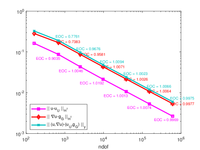
(a) $\mathbb{P}^{1}$ elements

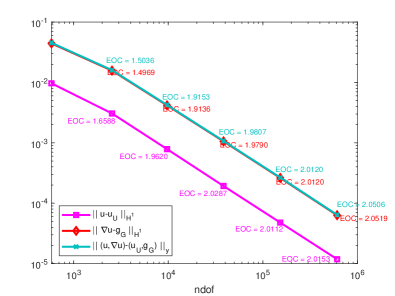
(b) $\mathbb{P}^{2}$ elements

Figure 1. Experimental order of convergence (EOC) for the Monge–Ampère test problem with $R=\sqrt{2}$.

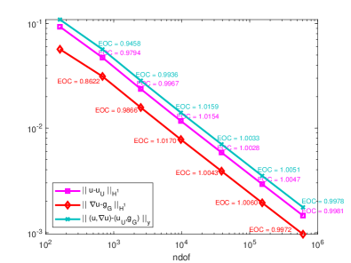
(a) $\mathbb{P}^{1}$ elements

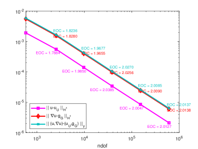
(b) $\mathbb{P}^{2}$ elements

Figure 2. Experimental order of convergence (EOC) for the Monge–Ampère test problem with $R=2$.

4.2. Problem (Hamilton–Jacobi–Bellman test)

Consider problem (27) and let $\mathcal{A}=[0,2\pi]$,

(36) $$\boldsymbol{{A}}^{\alpha}(\boldsymbol{x})=\begin{bmatrix}\cos(\alpha)&\sin(\alpha)\\ -\sin(\alpha)&\cos(\alpha)\end{bmatrix}\begin{bmatrix}1+(x_{1}^{2}+x_{2}^{2})&0.005\\ 0.005&1.01-(x_{1}^{2}+x_{2}^{2})\end{bmatrix}\begin{bmatrix}\cos(\alpha)&-\sin(\alpha)\\ \sin(\alpha)&\cos(\alpha)\end{bmatrix},$$

(37) $$\boldsymbol{b}^{\alpha}=0,\quad c^{\alpha}=2-0.5(\cos(2\alpha)+\sin(2\alpha)),\quad f^{\alpha}=\mathcal{{L}}^{\alpha}u-(1-\cos(2\alpha-\pi(x_{1}+x_{2}))),$$

with the exact solution

(38) $$u(\boldsymbol{x}):=\begin{cases}r(\boldsymbol{x})^{5/3}(1-r(\boldsymbol{x}))^{5/2}\sin(\varphi(\boldsymbol{x}))^{5/2}&\text{ if }0<r(\boldsymbol{x})\leqslant 1\text{ and },0<\varphi(\boldsymbol{x})<3\pi/2,\\ 0&\text{ otherwise, }\end{cases}$$

$(r(\boldsymbol{x}),\varphi(\boldsymbol{x}))$ are polar coordinates centered in the origin. One can check that the near degenerate diffusion $\boldsymbol{{A}}^{\alpha}$ together with $\boldsymbol{b}^{\alpha}$ and $c^{\alpha}$ satisfy the Cordes condition (3) with $\lambda=1$ and $\varepsilon=0.0032$. Note that $u\in\operatorname{H}^{s}$ for any $s<8/3$. As $u\in\operatorname{H}^{2}(\varOmega)$, we do not expect the advantage of the adaptive scheme over than the uniform refinement for $\operatorname{H}^{1}(\varOmega)$-norm of the error of $\mathsf{u}_{\mathbb{U}{}}$; it is shown in Figure 3b. But since $\nabla u$ does not have such smoothness, we observe the superiority of the adaptive scheme for $\operatorname{H}^{1}(\varOmega)$-norm of the error of $\boldsymbol{\mathsf{g}}{{}_{\mathbb{G}{}}}$ (and $\mathscr{{Y}}$-norm of the error of $(\mathsf{u}_{\mathbb{U}{}},\boldsymbol{\mathsf{g}}{{}_{\mathbb{G}{}}})$) in Figure 3c (and 3d).

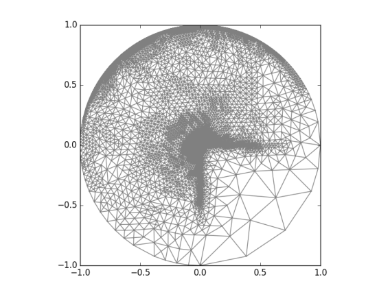
(a) Last mesh generated by the adaptive algorithm.

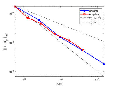
(b) Error $\left\|{u-\mathsf{u}_{\mathbb{U}{}}}\right\|_{\operatorname{H}^{1}(\varOmega)}$ convergence of uniform and adaptive methods.

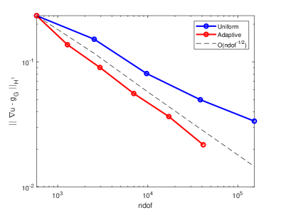
(c)

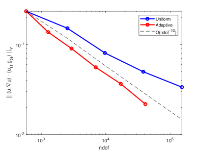
(d)

Figure 3. Mesh in 3a and 3b–3d show the convergence rate in both the uniform and adaptive refinement for the HJB test problem §4.2 with $\mathbb{P}^{2}$ elements. While the adaptive scheme does not yield any noticeable gain for the function value approximation ($\left\|{u-\mathsf{u}_{\mathbb{U}{}}}\right\|_{\operatorname{H}^{1}(\varOmega)}$), it does so in the reconstructed gradient ($\left\|{\nabla u-\boldsymbol{\mathsf{g}}{{}_{\mathbb{G}{}}}}\right\|_{\mathscr{{Y}}}$).

References

• Ciarlet [2002] Philippe G. Ciarlet. Finite Element Method for Elliptic Problems. Society for Industrial and Applied Mathematics, Philadelphia, PA, USA, 2002. ISBN 0898715148.
• Feng and Jensen [2017] Xiaobing Feng and Max Jensen. Convergent semi-Lagrangian methods for the Monge-Ampère equation on unstructured grids. SIAM Journal on Numerical Analysis, 55(2):691–712, 2017. ISSN 0036-1429. doi: 10.1137/16M1061709. URL https://epubs.siam.org/doi/10.1137/16M1061709.
• Gallistl and Süli [2019] Dietmar Gallistl and Endre Süli. Mixed Finite Element Approximation of the Hamilton–Jacobi–Bellman Equation with Cordes Coefficients. SIAM Journal on Numerical Analysis, 57(2):592–614, 01 2019. ISSN 0036-1429. doi: 10.1137/18M1192299. URL https://epubs.siam.org/doi/abs/10.1137/18M1192299.
• Ito and Kunisch [2008] Kazufumi Ito and Karl Kunisch. Lagrange multiplier approach to variational problems and applications. SIAM, Philadelphia, 2008. ISBN 978-0-89871-649-8. URL http://www.worldcat.org/oclc/884103565. OCLC: 884103565.
• Lakkis and Mousavi [2019] Omar Lakkis and Amireh Mousavi. A least-squares Galerkin approach to gradient and Hessian recovery for nondivergence-form elliptic equations. online preprint (under peer-review) 1909.00491, arXiv, 09 2019. URL https://arxiv.org/abs/1909.00491v1.
• Lakkis and Mousavi [2020] Omar Lakkis and Amireh Mousavi. A least-squares galerkin approach to gradient recovery for Hamilton-Jacobi-Bellman equations with cordes coefficients. in preparation, 2020.
• Lakkis and Pryer [2013] Omar Lakkis and Tristan Pryer. A finite element method for nonlinear elliptic problems. SIAM Journal on Scientific Computing, 35(4):A2025–A2045, 2013. doi: 10.1137/120887655. URL http://arxiv.org/abs/1103.2970.
• Smears and Süli [2014] Iain Smears and Endre Süli. Discontinuous Galerkin finite element approximation of Hamilton-Jacobi-Bellman equations with Cordes coefficients. SIAM J. Numer. Anal., 52(2):993–1016, 2014. ISSN 0036-1429. doi: 10.1137/130909536. URL https://epubs.siam.org/doi/10.1137/130909536.
• Smears and Süli [2016] Iain Smears and Endre Süli. Discontinuous Galerkin finite element methods for time-dependent Hamilton–Jacobi–Bellman equations with Cordes coefficients. Numerische Mathematik, 133(1):141–176, May 2016. ISSN 0029-599X, 0945-3245. doi: 10.1007/s00211-015-0741-6. URL http://arxiv.org/abs/1406.4839. arXiv: 1406.4839.