Efficient Fully Distribution-Free
Center-Outward Rank Tests
for Multiple-Output Regression
and MANOVA

Abstract

Extending rank-based inference to a multivariate setting such as multiple-output regression or MANOVA with unspecified $d$-dimensional error density has remained an open problem for more than half a century. None of the many solutions proposed so far is enjoying the combination of distribution-freeness and efficiency that makes rank-based inference a successful tool in the univariate setting. A concept of center-outward multivariate ranks and signs based on measure transportation ideas has been introduced recently. Center-outward ranks and signs are not only distribution-free but achieve in dimension $d>1$ the (essential) maximal ancillarity property of traditional univariate ranks. In the present case, we show that fully distribution-free testing procedures based on center-outward ranks can achieve parametric efficiency. We establish the Hájek representation and asymptotic normality results required in the construction of such tests in multiple-output regression and MANOVA models. Simulations and an empirical study demonstrate the excellent performance of the proposed procedures.

Keywords: Distribution-free tests; Multivariate ranks; Multivariate signs; Hájek representation.

1 Introduction

Linear models—regression (single- and multiple-output), Analysis of Variance (ANOVA and MANOVA)—are probably the most popular and most useful of all statistical models; they are found in the table of contents of all statistical textbooks and statistical softwares, and are part of daily statistical practice in all domains of application. The pseudo-Gaussian approach—Gaussian quasi maximum likelihood estimation and pseudo-Gaussian $F$ tests—is largely dominant in that context, on the ground that pseudo-Gaussian methods remain asymptotically valid under a broad class of non-Gaussian densities satisfying mild moment conditions. One should beware of excessive confidence in such asymptotics, though.

1.1 Pseudo-Gaussian tests

Let us concentrate on hypothesis testing. The problem with pseudo-Gaussian tests under unspecified noise density is twofold:

1. although pseudo-Gaussian tests are asymptotically valid under a broad range of non-Gaussian densities, that asymptotic validity is far from uniform: actually, in a semiparametric model with parameter $\theta$ where the underlying noise has unspecified density $f$ in some broad class $\cal F$ of densities, a sequence $\varphi^{(n)}$ of tests of the null hypothesis $\theta=\theta_{0}$ has asymptotic level $\alpha$ iff $\lim_{n\to\infty}\sup_{f\in{\cal F}}{\rm E}_{\theta_{0},f}[\varphi^{(n)}]\leq\alpha$, whereas pseudo-Gaussian tests $\varphi^{(n)}_{\cal G}$ only satisfy the pointwise condition $\lim_{n\to\infty}{\rm E}_{\theta_{0},f}[\varphi^{(n)}_{\cal G}]\leq\alpha$ for all $f\in{\cal F}$;

2. still for fixed $n$, the performance of pseudo-Gaussian tests may rapidly deteriorate away from the Gaussian.

Appendix A.1 illustrates these pitfalls in the case of Hotelling’s bivariate two-sample test.

1.2 Rank-based tests

A natural way to restore uniform asymptotics, thereby solving the validity problem in (a) consists in resorting to distribution-free tests, and this is how rank tests enter the picture. Rank-based testing methods have been quite successful in testing problems for single-ouput regression and linear models such as ANOVA (see the classical monographs by Hájek and Šidák, (1967), Randles and Wolfe, (1979) or Puri and Sen, (1985)) and univariate linear time series (Hallin et al., (1985), Koul and Saleh, (1993), Hallin and Puri, (1994)). Being distribution-free, rank tests remain valid over the full class of absolutely continuous distributions. In linear models (this includes testing for single-output regression slopes, testing for treatment effects in analysis of variance, testing against location shifts in two-sample problems) and ARMA time series, they do reach parametric or semiparametric efficiency bounds at given reference densities, thus reconciling the conflicting objectives of robustness and efficiency. The celebrated Chernoff-Savage result (Chernoff and Savage, (1958) and, for time-series, Hallin, (1994)) moreover indicates that, far from losing power with respect to their pseudo-Gaussian counterparts, rank tests strictly dominate them under any non-Gaussian density $f$, making the latter non-admissible.

Extending these attractive features to a multivariate (multiple-output) context, of course, is highly desirable and the problem of defining multivariate concepts of ranks has been a long-standing open problem, for which many solutions have been proposed in the literature. Puri and Sen, (1971) for a variety of problems in multivariate analysis (including multiple-output regression and MANOVA) and Hallin et al., (1989) for VARMA time series models construct tests based on it componentwise ranks which, however, fail to be distribution-free. Building upon an ingenious multivariate extension of the L₁ definition of quantiles, Oja, (1999, 2010) defines the so-called spatial ranks; the resulting tests are neither distribution-free nor efficient. Tests based on the ranks of various concepts of statistical depth also have been proposed (Liu, (1992), Liu and Singh, (1993), Zuo and He, (2006)). While distribution-free, these ranks are failing to exploit any directional information, and hence typically do not allow for any type of asymptotic efficiency. As for the tests based on the Mahalanobis ranks and signs proposed by Hallin and Paindaveine, 2002a , Hallin and Paindaveine, 2002b , Hallin and Paindaveine, (2004, 2005), they do achieve, within the class of linear models and linear time series with elliptical densities, parametric or semiparametric efficiency at correctly specified elliptical reference densities; their distribution-freeness, hence their validity, unfortunately, is limited to the class of elliptical distributions.

Inspired by measure transportation ideas, a new concept of ranks and signs for multivariate observations has been introduced recently under the name of Monge-Kantorovich ranks and signs in Chernozhukov et al., (2017), under the name of center-outward ranks and signs in Hallin, (2017) and Hallin et al., 2021a , along with the related population concepts of center-outward distribution and quantile functions. Unlike earlier concepts, these ranks and signs extend to dimension $d>1$ the essential maximal ancillarity property (see Section 2.4 and Appendices D1 and D.2 of Hallin et al., 2021a ) of univariate ranks; the corresponding empirical center-outward distribution functions, moreover, satisfy a Glivenko-Cantelli result.

Center-outward ranks and signs have been successfully applied (Boeckel et al., (2018), Deb and Sen, (2019), Ghosal and Sen, (2019), Shi et al., 2021a , Shi et al., 2021b , Shi et al., 2021c ) in the construction of distribution-free tests of independence between random vectors and multivariate goodness-of-fit; applications to the study of tail behavior and extremes can be found in De Valk and Segers, (2018); Beirlant et al., (2020) are using the related center-outward empirical quantiles in the analysis of multivariate risk; Hallin et al., 2021b , Hallin et al., 2020b are proposing center-outward tests and R-estimators for VAR and VARMA time series models with unspecified innovation densities. We refer to Hallin, (2022) for a review. The present paper goes one step further in the direction of a toolkit of distribution-free tests for multiple-output multivariate analysis by deriving a Hájek-type asymptotic representation result for linear center-outward rank statistics. Asymptotic normality follows as a corollary, from which center-outward rank tests are constructed for multiple-output regression models (including, as special cases, MANOVA and two-sample location models). Those tests are fully distribution-free, hence valid, over the entire family of absolutely continuous distributions; for adequate choice of the scores, parametric efficiency is attained at chosen densities. Since this paper was written (Hallin et al., 2020a, ), some further results (among them, partial Chernoff-Savage and Hodges-Lehmann properties) on the particular case of the two-sample location problem have been obtained by Deb et al., (2021); see Hallin and Mordant, (2021) for some numerical comparisons with the tests presented here.

1.3 A motivating example

The importance of center-outward rank tests in daily statistical practice is illustrated with the following real-life motivating example. The Wisconsin Diagnostic Breast Cancer data (WDBC; dataset available at Machine Learning Repository Dua and Graff, (2017)), first analyzed in Street et al., (1993) in a classification context, contains records on $n=569$ patients from two groups—benign or malignant tumor diagnosis. For each patient, several features were recorded from the digitized image of a fine needle aspirate of the breast mass, resulting in $d=30$ variables, labeled V1–V30. The two groups of patients are well separated: the two-sample Hotelling test in dimension $d=~{}\!30$ very significantly rejects the null hypothesis of equal locations (the R program delivers a $p$-value 0.000, meaning that the actual $p$-value is less than $10^{-22}$!).So does the Wilcoxon center-outward rank test.

In real life, however, diagnoses requiring 30 clinical measurements are highly impractical and costly. Reducing that number from 30 to 3 or 4 without losing diagnostic efficiency is an important issue. Unfortunately, when restricted to subsets of three or four variables, the Hotelling test typically is inconclusive. Consider, for instance, the subset consisting of V12 (mean of fractal dimension), V14 (standard error of texture), V21 (standard error of symmetry), and V22 (standard error of fractal dimension). Figure 1 shows bivariate scatterplots and histograms for these four variables, revealing skewness in all univariate marginals and deviations from elliptical symmetry in bivariate marginals.

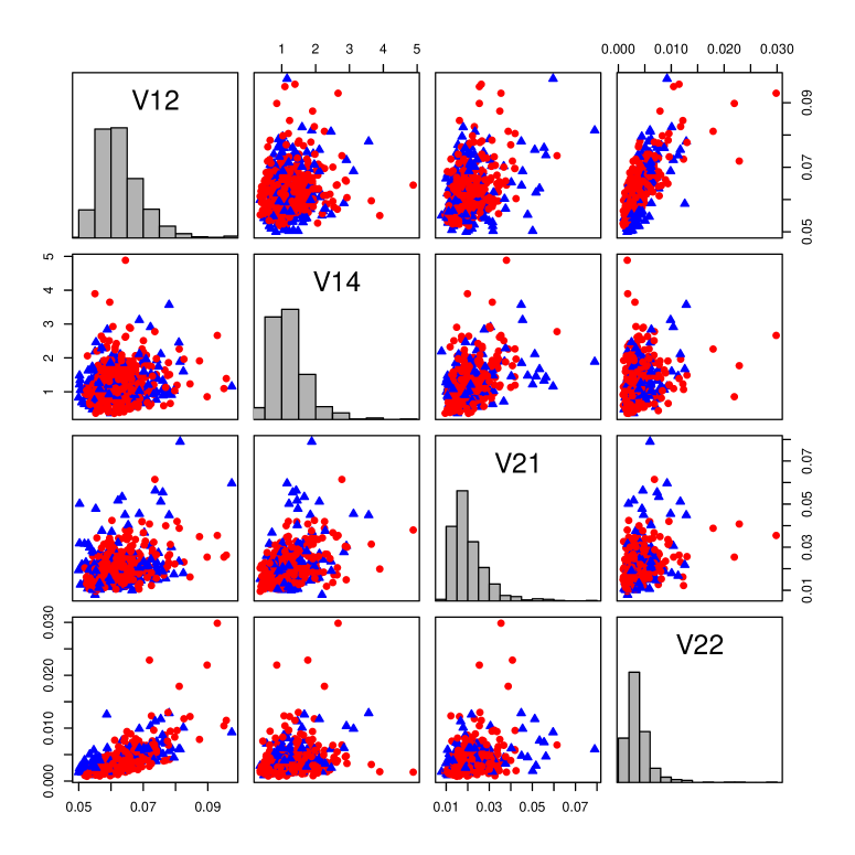
Figure 1: Wisconsin Diagnostic Breast Cancer (WDBC) data: bivariate scatterplots and univariate histograms for mean fractal dimension (V12), standard error of texture (V14), standard error of symmetry (V21), and standard error of fractal dimension (V22) in 212 malignant patients (triangles) and 357 benign patients (circles).

The Hotelling and Wilcoxon center-outward rank tests (see Section 5.3.1 for a precise description) have been performed for the corresponding four-dimensional dataset and all its three-dimensional marginals; $p$-values are shown in Table 1. With $p$-value 0.0090, the Wilcoxon test in dimension 4 is significant at 5% and 1% levels, while Hotelling (with $p$-value 0.0595) is not. Turning to dimension 3, Wilcoxon is always significant at 5% level (at 1% level in all cases but one), while Hotelling never rejects on 1%. The most spectacular case is that of the subset $\{V12,V14,V21\}$ where Wilcoxon and Hotelling yield $p$-values 0.0327 and 0.9899, respectively.

Variables	(12,14,21, 22)	(12,14,21)	(12,14,22)	(12,21,22)	(14,21,22)
Hotelling	0.0595	0.9899	0.0299	0.0346	0.2136
c-o Wilcoxon	0.0090	0.0327	0.0007	0.0000	0.0018

Table 1: Wisconsin Diagnostic Breast Cancer (WDBC) data: $p$-values of the two-sample location Hotelling and center-outward Wilcoxon rank tests for the 4-dimensional marginal WDBC data corresponding to the set of variables $\{$V12,V14,VV21,V22$\}$ and its 3-dimensional subsets.

Such discrepancies most likely originate in the skewness, non-ellipticity and/or the heavy tails of the observations; their impact in terms of diagnostic power may have crucial consequences.

1.4 Outline of the paper

The paper is organized as follows. Section 2 briefly describes the main tools to be used: center-outward distribution and quantile functions (Section 2.1) and their empirical counterparts, the center-outward ranks and signs (Section 2.2). The main properties of these concepts are summarized in Section 2.3 (Proposition 2.1); their invariance/equivariance properties are established in Proposition 2.2. Section 3 is entirely devoted to the key theoretical results of this paper, which extend and generalize the classical approach by Hájek and Šidák (1967): a Hájek-type asymptotic representation for multivariate center-outward linear rank statistics and the resulting asymptotic normality result. Section 4.1 describes the multiple-output regression model to be considered throughout, which contains, as particular cases, the two-sample location and MANOVA models, of obvious practical importance. Local asymptotic normality is established in Section 4.2 for this model under general error densities (Proposition 4.1) and, for the purpose of future comparisons, for the particular case of elliptical distributions (Proposition 4.2). The center-outward rank tests we are proposing are described in Section 5.2, along with (Corollary 5.2) their local asymptotic optimality properties. Due to their importance in applications, the particular cases of the hypotheses of equal locations in the two-sample problem and no treatment effect in MANOVA are considered in Section 5.3. Sections 6.1 and 6.2 propose some simple choices of score functions, extending the classical median-test-score (based on center-outward signs only), Wilcoxon, and van der Waerden (normal-score) tests. Section 6.3 discusses affine invariance issues. Section 7 is devoted to a Monte Carlo exploration, in dimension $d=2$, of the finite-sample performance of our rank tests which appear to outperform their competitors in non-elliptical situations while performing equally well under ellipticity. Section 7.3 presents an archaeological MANOVA application in dimension $d=4$; while traditional MANOVA methods cannot reject the hypothesis of no treatment effect, our fully distribution-free center-outward rank-based test rejects it quite significantly, which might lead to revising some of the conclusions (Phelps et al., , 2016) on Middle-East economic exchanges between Egypt and Syro-Palestine in the Byzantine-Islamic transition period. All proofs are concentrated in an online appendix where we also provide simulations in dimension $d=6$.

2 Center-outward ranks and signs in $\mathbb{R}^{d}$

2.1 Center-outward distribution functions

Throughout, denote by $\mathbf{Z}^{(n)}$ a triangular array $(\mathbf{Z}_{1}^{(n)},\dots,\mathbf{Z}_{n}^{(n)})$, $n\in\mathbb{N}$ of i.i.d. $d$-dimensional random vectors with distribution $\mathrm{P}$ in the family ${\mathcal{P}}_{d}$ of absolutely continuous distributions on $\mathbbm{R}^{d}$. The notation $\overline{\text{spt}}({\rm P})$ is used for the support of ${\rm P}$, ${\text{spt}}({\rm P})$ for its interior. The open (resp. closed) unit ball and the unit hypersphere in ${\mathbb{R}}^{d}$ are denoted by ${\mathbb{S}_{d}}$ (resp. $\overline{{\mathbb{S}}}_{d}$) and ${\mathcal{S}_{d-1}}$, respectively; ${\rm U}_{d}$ stands for the spherical uniform distribution over ${\mathbb{S}_{d}}$, $\mu_{d}$ for the Lebesgue measure over $\mathbb{R}^{d}$; ${\bf I}_{d}$ is the $d\times d$ unit matrix, ${\bf 1}_{A}$ the indicator of the Borel set $A$.

The definition of the center-outward distribution function of $\rm P$ is particularly simple for ${\rm P}$ in the so-called class ${\cal P}^{+}_{d}$ of distributions with nonvanishing densities—namely, the class of all distributions with density $f:={\rm dP}/{\rm d}\mu_{d}$ such that, for all $D\in\mathbb{R}^{+}$, there exist constants $\lambda^{-}_{D;\mathrm{P}}$ and $\lambda^{+}_{D;\mathrm{P}}$ satisfying $0<\lambda^{-}_{D;\mathrm{P}}\leq f({\bf z})\leq\lambda^{+}_{D;\mathrm{P}}<\infty$ for all $\bf z$ with $\|{\bf z}\|\leq D$ (so that spt$({\rm P})=\mathbb{R}^{d}$ and $\rm P$-a.s. is equivalent to $\mu_{d}$-a.e.). The main result in McCann, (1995) then implies the existence of an a.e. unique convex lower semi-continuous function $\varphi:~{}\!\mathbb{R}^{d}\to~{}\!\mathbb{R}$ with gradient $\nabla\varphi$ such that $\nabla\varphi\#{\rm P}={\rm U}_{d}$—we borrow from measure transportation the convenient notation $T\#\mathrm{P}$ ($T\!:\mathbb{R}^{d}\to~{}\!\mathbb{R}^{d}$ pushes $\mathrm{P}$ forward to $T\#\mathrm{P}$) for the distribution under ${\bf Z}\sim\mathrm{P}$ of $T({\bf Z})$. Call ${\bf F}_{\scriptscriptstyle\pm}:=\nabla\varphi$ the center-outward distribution function of $\rm P$. It follows from Figalli, (2018) that ${\bf F}_{\scriptscriptstyle\pm}$ defines a homeomorphism between the punctured unit ball ${\mathbb{S}}_{d}\!\setminus\!\{{\bf 0}\}$ and its image $\mathbb{R}^{d}\!\setminus\!{\bf F}_{\scriptscriptstyle\pm}^{-1}({\bf 0})$: call ${\bf Q}_{\scriptscriptstyle\pm}:{\bf u}\mapsto{\bf Q}_{\scriptscriptstyle\pm}({\bf u}):={\bf F}_{\scriptscriptstyle\pm}^{-1}({\bf u})$, ${\bf u}\neq{\bf 0}$ the center-outward quantile function. Figalli, (2018) also shows that, defining ${\bf Q}_{\scriptscriptstyle\pm}({\bf 0}):={\bf F}_{\scriptscriptstyle\pm}^{-1}({\bf 0})$ yields a convex and compact subset with Lebesgue measure zero in $\mathbb{R}^{d}$, the center-outward median set of $\rm P$.

All the intuition and all the properties of center-outward distribution and quantile functions hold for ${\rm P}\in{\cal P}^{+}_{d}$; this special case is the one considered in Hallin, (2017). A more general case is addressed in del Barrio et al., (2020) and Hallin et al., 2021a where we refer to for details, but requires more technical definitions, which we are skipping here. Note, however, that while some statements below only hold under ${\rm P}\in{\cal P}_{d}^{+}$, many others (including validity), due to distribution-freeness, can be made under the very general condition ${\rm P}\in{\cal P}_{d}$.

2.2 Center-outward ranks and signs

Except for a few particular cases such as spherical distributions, the above definitions are not meant for an analytical derivation of ${\bf F}_{{\scriptscriptstyle\pm}}$ and ${\bf Q}_{{\scriptscriptstyle\pm}}$ which typically involves Monge-Ampère equations; in particular, no closed forms of ${\bf F}_{{\scriptscriptstyle\pm}}$ and ${\bf Q}_{{\scriptscriptstyle\pm}}$ are known for non-spherical elliptical distributions. Estimation is possible, though, via their empirical counterparts ${\bf F}_{\scriptscriptstyle\pm}^{(n)}$ and ${\bf Q}_{\scriptscriptstyle\pm}^{(n)}$, based on center-outward ranks and signs, which we now describe.

Associated with the $n$-tuple $\mathbf{Z}_{1}^{(n)},\dots,\mathbf{Z}_{n}^{(n)}$, the empirical center-outward distribution function ${\bf F}_{\scriptscriptstyle\pm}^{(n)}$ is mapping $\mathbf{Z}_{1}^{(n)},\dots,\mathbf{Z}_{n}^{(n)}$ to a “regular” grid $\mathfrak{G}_{n}$ of the unit ball ${\mathbb{S}}_{d}$. That grid $\mathfrak{G}_{n}$ is obtained as follows:

1. first factorize $n$ into $n=n_{R}n_{S}+n_{0}$, with $0\leq n_{0}<\min(n_{R},n_{S})$;

2. next consider a “regular array” $\mathfrak{S}_{n_{S}}:=\{{\bf s}^{n_{S}}_{1},\ldots,{\bf s}^{n_{S}}_{n_{S}}\}$ of $n_{S}$ points on the sphere ${\cal S}_{d-1}$ (see the comment below);

3. finally, the grid consists in the collection $\mathfrak{G}_{n}$ of the $n_{R}n_{S}$ points $\mathfrak{g}$ of the form

   $$\big{(}r/\big{(}n_{R}+1\big{)}\big{)}{\bf s}^{n_{S}}_{s},\quad r=1,\ldots,n_{R},\ \ s=1,\ldots,n_{S},\vspace{-1mm}$$

   along with ($n_{0}$ copies of) the origin in case $n_{0}\neq 0$: a total number $n-(n_{0}-1)$ or $n$ of distinct points, thus, according as $n_{0}>0$ or $n_{0}=0$.

By “regular” we mean “as uniform as possible”, in the sense, for example, of the low-discrepancy sequences of the type considered in numerical integration and Monte-Carlo methods (see, e.g., Niederreiter, (1992), Judd, (1998), or Santner et al., (2003)). The only mathematical requirement needed for Proposition 2.1 below is the weak convergence, as $n\to\infty$, of the uniform discrete distribution over $\mathfrak{S}_{n}$ to the uniform distribution over ${\mathbb{S}}_{d}$; all sequences $\mathfrak{S}_{n}$ satisfying that requirement yield the same asymptotic results. A uniform i.i.d. sample of points over ${\mathbb{S}}_{d}$, for example, satisfies the requirement but fails to produce mutually independent ranks and signs; moreover, one easily can construct arrays that are “more regular” than an i.i.d. one. For instance, one could see that $n_{S}$ or $n_{S}-1$ of the points ${\bf s}^{n_{S}}_{s}$ in $\mathfrak{S}_{n}$ are such that $-\,{\bf s}^{n_{S}}_{s}$ also belongs to $\mathfrak{S}_{n_{S}}$, so that $\|\sum_{s=1}^{n_{S}}{\bf s}^{n_{S}}_{s}\|$ is 0 or 1 according as $n_{S}$ is even or odd. One also could consider factorizations of theform $n=n_{R}n_{S}+n_{0}$ with $n_{S}$ even and $0\leq n_{0}<\min(2n_{R},n_{S})$, then require $\mathfrak{S}_{n}$ to be symmetric with respect to the origin, automatically yielding $\sum_{s=1}^{n_{S}}{\bf s}^{n_{S}}_{s}={\bf 0}$.

The empirical counterpart ${\bf F}_{\scriptscriptstyle\pm}^{(n)}$ of ${\bf F}_{\scriptscriptstyle\pm}$ is defined as the (bijective, once the origin is given multiplicity $n_{0}$) mapping from $\mathbf{Z}_{1}^{(n)},\dots,\mathbf{Z}_{n}^{(n)}$ to the grid $\mathfrak{G}_{n}$ that minimizes the sum of squared Euclidean distances $\sum_{i=1}^{n}\big{\|}{\bf F}_{\scriptscriptstyle\pm}^{(n)}(\mathbf{Z}_{i}^{(n)})-\mathbf{Z}_{i}^{(n)}\big{\|}^{2}$. That mapping is unique with probability one; in practice, it is obtained via a simple optimal assignment (pairing) algorithm (a linear program; see Section 4 of Hallin, (2017) for details).

Call center-outward rank of $\mathbf{Z}_{i}^{(n)}$ the integer (in $\{1,\ldots,n_{R}\}$ or $\{0,\ldots,n_{R}\}$ according as $n_{0}=0$ or not) $R^{(n)}_{i;{{{\scriptscriptstyle\pm}}s}}:=(n_{R}+1)\big{\|}{\bf F}_{\scriptscriptstyle\pm}^{(n)}(\mathbf{Z}_{i}^{(n)})\big{\|}$ and center-outward sign of $\mathbf{Z}_{i}^{(n)}$ the unit vector ${\bf S}^{(n)}_{i;{{\scriptscriptstyle\pm}}}:={\bf F}_{\scriptscriptstyle\pm}^{(n)}(\mathbf{Z}_{i}^{(n)})/\big{\|}{\bf F}_{\scriptscriptstyle\pm}^{(n)}(\mathbf{Z}_{i}^{(n)})\big{\|}$ for ${\bf F}_{\scriptscriptstyle\pm}^{(n)}(\mathbf{Z}_{i}^{(n)})\neq{\bf 0}$; for ${\bf F}_{\scriptscriptstyle\pm}^{(n)}(\mathbf{Z}_{i}^{(n)})={\bf 0}$, put ${\bf S}^{(n)}_{i;{{{\scriptscriptstyle\pm}}s}}={\bf 0}$.

Some desirable finite-sample properties, such as strict independence between the ranks and the signs, only hold for $n_{0}=0$ or 1, due to the fact that the mapping from the sample to the grid is no longer injective for $n_{0}\geq 2$. This, which has no asymptotic consequences (since the number $n_{0}$ of tied values involved is $o(n)$ as $n\to\infty$), is easily taken care of by the following tie-breaking device:

1. randomly select $n_{0}$ directions ${\bf s}^{0}_{1},\ldots,{\bf s}^{0}_{n_{0}}$ in $\mathfrak{S}_{n_{S}}$, then

2. replace the $n_{0}$ copies of the origin with the new gridpoints $\frac{1}{2(n_{R}+1)}{\bf s}^{0}_{1},\ldots,\frac{1}{2(n_{R}+1)}{\bf s}^{0}_{n_{0}}$.

The resulting grid (for simplicity, the same notation ${\mathfrak{G}}_{n}$ is used) no longer has multiple points, and the optimal pairing between the sample and the grid is bijective; the $n_{0}$ smallest ranks, however, take the non-integer value $1/2$. Again, this tie-breaking device has no influence on asymptotic results.

2.3 Main properties

This section summarizes the main properties of the concepts defined in Sections 2.1 and 2.2; further properties and a proof for Proposition 2.1 can be found in Hallin et al., 2021a .

Proposition 2.1.

Let ${\bf F}_{{\scriptscriptstyle\pm}}$ denote the center-outward distribution function of ${\rm P}\in{\cal P}_{d}$. Then,

1. ${\bf F}_{{\scriptscriptstyle\pm}}$ is a probability integral transformation of $\mathbb{R}^{d}$: namely, ${\bf Z}\sim{\rm P}$ iff ${\bf F}_{{\scriptscriptstyle\pm}}({\bf Z})\sim{\rm U}_{d}$; by construction, $\|{\bf F}_{{\scriptscriptstyle\pm}}({\bf Z})\|$ is uniform over the interval $[0,1]$, ${\bf F}_{{\scriptscriptstyle\pm}}({\bf Z})/\|{\bf F}_{{\scriptscriptstyle\pm}}({\bf Z})\|$ uniform over the sphere ${\cal S}_{d-1}$, and they are mutually independent.

Let ${\bf Z}^{(n)}_{i},\ldots,{\bf Z}^{(n)}_{i}$ be i.i.d. with distribution ${\rm P}\in{\mathcal{P}}_{d}$ and center-outward distribution function ${\bf F}_{{\scriptscriptstyle\pm}}$. Then,

1. $\big{(}{\bf F}^{(n)}_{{\scriptscriptstyle\pm}}({\bf Z}^{(n)}_{1}),\ldots,{\bf F}^{(n)}_{{\scriptscriptstyle\pm}}({\bf Z}^{(n)}_{n})\big{)}$ is uniformly distributed over the $n!/n_{0}!$ permutations with repetitions of the gridpoints in $\mathfrak{G}_{n}$ with the origin counted as $n_{0}$ indistinguishable points (resp. the $n!$ permutations of $\mathfrak{G}_{n}$ if either $n_{0}\leq 1$ or the tie-breaking device described in Section 2.2 is adopted);

2. if either $n_{0}=0$ or the tie-breaking device described in Section 2.2 is adopted, the $n$-tuple of center-outward ranks $\big{(}R^{(n)}_{1;{\scriptscriptstyle\pm}},\ldots,R^{(n)}_{n;{\scriptscriptstyle\pm}}\big{)}$ and the $n$-tuple of center-outward signs $\big{(}{\bf S}^{(n)}_{1;{\scriptscriptstyle\pm}},\ldots,{\bf S}^{(n)}_{n;{\scriptscriptstyle\pm}}\big{)}$ are mutually independent;

3. if either $n_{0}\leq 1$ or the tie-breaking device described in Section 2.2 is adopted, the $n$-tuple $\big{(}{\bf F}^{(n)}_{{\scriptscriptstyle\pm}}({\bf Z}^{(n)}_{1}),\ldots,{\bf F}^{(n)}_{{\scriptscriptstyle\pm}}({\bf Z}^{(n)}_{n})\big{)}$ is essentially maximal ancillary.

Assuming, moreover, that ${\rm P}\in{\mathcal{P}}_{d}^{+}$,

1. (Glivenko-Cantelli) $\displaystyle{\max_{1\leq i\leq n}}\Big{\|}{\bf F}^{(n)}_{{\scriptscriptstyle\pm}}({\bf Z}^{(n)}_{i})-{\bf F}_{{\scriptscriptstyle\pm}}({\bf Z}^{(n)}_{i})\Big{\|}\rightarrow 0$ a.s. as $n\to\infty$.

Center-outward distribution functions, ranks, and signs also inherit, from the invariance features of Euclidean distances, elementary but quite remarkable invariance and equivariance properties under orthogonal transformations. Denote by ${\bf F}^{{\bf Z}}_{{\scriptscriptstyle\pm}}$ the center-outward distribution function of $\bf Z$ and by ${\bf F}^{{\bf Z};(n)}_{{\scriptscriptstyle\pm}}$ the empirical distribution function of a sample ${\bf Z}_{1},\ldots,{\bf Z}_{n}$ associated with a grid $\mathfrak{G}_{n}$.

Proposition 2.2.

Let $\boldsymbol{\mu}\in\mathbb{R}^{d}$ and denote by ${\bf O}$ a $d\times d$ orthogonal matrix. Then,

1. ${\bf F}^{\boldsymbol{\mu}+{\bf O}{\bf Z}}_{{\scriptscriptstyle\pm}}(\boldsymbol{\mu}+{\bf O}{\bf z})={\bf O}{\bf F}^{\bf Z}_{{\scriptscriptstyle\pm}}({\bf z})$, ${\bf z}\in\mathbb{R}^{d}$;

2. denoting by ${\bf F}^{\boldsymbol{\mu}+{\bf O}{\bf Z};(n)}_{{\scriptscriptstyle\pm}}$the empirical distribution function of the sample $\boldsymbol{\mu}+{\bf O}{\bf Z}_{1},\ldots,\boldsymbol{\mu}+~{}\!{\bf O}{\bf Z}_{n}$ associated with the grid ${\bf O}\mathfrak{G}_{n}$ (hence, by ${\bf F}^{{\bf Z};(n)}_{{\scriptscriptstyle\pm}}$ the empirical distribution function of the sample ${\bf Z}_{1},\ldots,{\bf Z}_{n}$ associated with the grid $\mathfrak{G}_{n}$),

$${\bf F}^{\boldsymbol{\mu}+{\bf O}{\bf Z};(n)}_{{\scriptscriptstyle\pm}}(\boldsymbol{\mu}+{\bf O}{\bf Z}_{i})={\bf O}{\bf F}^{{\bf Z};(n)}_{{\scriptscriptstyle\pm}}({\bf Z}_{i}),\quad i=1,\ldots,n;$$ (2.1)

1. the center-outward ranks $R^{(n)}_{i;{{\scriptscriptstyle\pm}}}$ and the cosines ${\bf S}_{i;{{\scriptscriptstyle\pm}}}^{(n)\prime}{\bf S}_{j;{{\scriptscriptstyle\pm}}}^{(n)}$ computed from the sample ${\bf Z}_{1},\ldots,{\bf Z}_{n}$ and the grid $\mathfrak{G}_{n}$ are the same as those computed from the sample $\boldsymbol{\mu}+{\bf O}{\bf Z}_{1},\ldots,\boldsymbol{\mu}+{\bf O}{\bf Z}_{n}$ and the grid ${\bf O}\mathfrak{G}_{n}$.

See Appendix A.2 for the proof.

These orthogonal equivariance and invariance properties, however, do not extend to non-orthogonal affine transformations.

3 Hájek representation and asymptotic normality

As in Hájek and Šidák (1967), the rank-based statistics to be used in this context are quadratic forms in vectors of linear rank statistics—involving center-outward ranks and signs instead of ordinary ranks, though. Fundamental in Hájek’s approach is an asymptotic representation result establishing the asymptotic equivalence between linear rank statistics and sums of independent variables. We start with a center-outward version of that result; asymptotic normality follows as a corollary.

3.1 Linear center-outward rank statistics

Linear rank statistics in this context depend on a score function ${\bf J}:{\mathbb{S}_{d}}\to\mathbbm{R}^{d}$ and are indexed by triangular arrays $\{c^{(n)}_{1},\ldots,c^{(n)}_{n}\}$ of real numbers (regression constants). On those score functions and regression constants we are making the following assumptions.

Assumption 3.1.

1. ${\bf J}:{\mathbb{S}_{d}}\to\mathbbm{R}^{d}$ is continuous over ${\mathbb{S}_{d}}$;

2. for any sequence ${\mathfrak{s}}^{(n)}=\{{\bf s}^{(n)}_{1},\ldots,{\bf s}^{(n)}_{n}\}$ of $n$-tuples in ${\mathbb{S}_{d}}$ such that the uniform discrete distribution over ${\mathfrak{s}}^{(n)}$ converges weakly to ${\rm U}_{d}$ as $n\to~{}\!\infty$,

   $$\lim_{n\to\infty}n^{-1}\text{\rm tr}\sum_{r=1}^{n}{\bf J}({\bf s}^{(n)}_{r}){\bf J}^{\prime}({\bf s}^{(n)}_{r})=\text{\rm tr}\int_{\mathbb{S}_{d}}{\bf J}({\bf u}){\bf J}^{\prime}({\bf u})\,{\mathrm{d}}{\rm U}_{d}$$ (3.2)

   where $\int_{\mathbb{S}_{d}}{\bf J}({\bf u}){\bf J}^{\prime}({\bf u})\,{\mathrm{d}}{\rm U}_{d}<\infty$ has full rank.

As we shall see, a special role is played, in relation with spherical distributions, by score functions of the form

$${\mathbf{J}}({\bf u}):=J(\|{\bf u}\|)\frac{{\bf u}}{\|{\bf u}\|}{\bf 1}_{[\|{\bf u}\|\neq 0]}\qquad{\bf u}\in\mathbb{S}_{d}$$ (3.3)

for some function $J:[0,1)\to\mathbbm{R}$. Assumption 3.1 then holds if (i) $J$ is continuous and (ii)

$$0<{\lim_{n\to\infty}n^{-1}\sum_{r=1}^{n}J^{2}\big{(}r/(n+1)\big{)}=\int_{0}^{1}J^{2}(u)\,{\mathrm{d}}u<\infty}$$ (3.4)

(a sufficient condition for (3.4) is the traditional assumption that $J$ has bounded variation, i.e., is the difference of two nondecreasing functions). Both (3.2) and (3.4) extend the conditions on univariate scores in Section V.1.6 of Hájek and Šidák, (1967).

As for the regression constants, we assume that the classical Noether conditions hold.

Assumption 3.2.

The $c^{(n)}_{i}$’s are not all equal (for given $n$) and satisfy

$$\sum_{i=1}^{n}(c^{(n)}_{i}-\bar{c}^{(n)})^{2}/{\max\limits_{1\leq i\leq n}(c^{(n)}_{i}-\bar{c}^{(n)})^{2}}\longrightarrow\infty\quad\text{ as }n\to\infty\vspace{-2mm}$$ (3.5)

where ${\bar{c}^{(n)}:=n^{-1}\sum_{i=1}^{n}c^{(n)}_{i}}$.

Associated with the score functions ${\bf J}$, consider the $d$-dimensional statistics

$$\stackunder[1pt]{\mathbf{T}}{\scriptscriptstyle\thicksim}^{(n)}_{a} ={\Big{(}{\sum_{i=1}^{n}(c_{i}^{(n)}-\bar{c}^{(n)})^{2}}\Big{)}^{-1/2}}\sum_{i=1}^{n}(c_{i}^{(n)}-\bar{c}^{(n)}){\mathbf{J}}(\mathbf{F}_{{\scriptscriptstyle\pm}}^{(n)}(\mathbf{Z}_{i}^{(n)})),$$ (3.6)

$$\stackunder[1pt]{\mathbf{T}}{\scriptscriptstyle\thicksim}^{(n)}_{e} :={\Big{(}{\sum_{i=1}^{n}(c_{i}^{(n)}-\bar{c}^{(n)})^{2}}\Big{)}^{-1/2}}\sum_{i=1}^{n}(c_{i}^{(n)}-\bar{c}^{(n)})\mathrm{E}\left[{\mathbf{J}}({\bf F}_{\scriptscriptstyle\pm}(\mathbf{Z}_{i}^{(n)}))\bigg{|}\mathbf{F}_{{\scriptscriptstyle\pm}}^{(n)}(\mathbf{Z}_{i}^{(n)})\right],$$

and

$${\mathbf{T}}^{(n)} :={\Big{(}{\sum_{i=1}^{n}(c_{i}^{(n)}-\bar{c}^{(n)})^{2}}\Big{)}^{-1/2}}\sum_{i=1}^{n}(c_{i}^{(n)}-\bar{c}^{(n)}){\mathbf{J}}({\bf F}_{\scriptscriptstyle\pm}(\mathbf{Z}_{i}^{(n)})).$$

Adopting Hájek’s terminology, call $\stackunder[1pt]{\mathbf{T}}{\scriptscriptstyle\thicksim}^{(n)}_{a}$ an approximate-score linear rank statistic and $\stackunder[1pt]{\mathbf{T}}{\scriptscriptstyle\thicksim}^{(n)}_{e}$ an exact-score linear rank statistic. As we shall see, both $\stackunder[1pt]{\mathbf{T}}{\scriptscriptstyle\thicksim}^{(n)}_{a}$ and $\stackunder[1pt]{\mathbf{T}}{\scriptscriptstyle\thicksim}^{(n)}_{e}$ admit the same asymptotic representation ${\mathbf{T}}^{(n)}\!$, hence are asymptotically equivalent. For score functions of the form (3.3), we have

$$\stackunder[1pt]{\mathbf{T}}{\scriptscriptstyle\thicksim}^{(n)}_{a}={\Big{(}{\sum_{i=1}^{n}(c_{i}^{(n)}-\bar{c}^{(n)})^{2}}\Big{)}^{-1/2}}\sum_{i=1}^{n}(c_{i}^{(n)}-\bar{c}^{(n)})J\Big{(}\frac{R^{(n)}_{i;{{\scriptscriptstyle\pm}}}}{n_{R}+1}\Big{)}{\bf S}^{(n)}_{i;{{\scriptscriptstyle\pm}}},$$

$$\stackunder[1pt]{\mathbf{T}}{\scriptscriptstyle\thicksim}^{(n)}_{e}= {\Big{(}{\sum_{i=1}^{n}(c_{i}^{(n)}-\bar{c}^{(n)})^{2}}\Big{)}^{-1/2}}$$

$$\times\sum_{i=1}^{n}(c_{i}^{(n)}-\bar{c}^{(n)})\mathrm{E}\left[J\big{(}\big{\|}{\bf F}_{\scriptscriptstyle\pm}(\mathbf{Z}_{i}^{(n)})\big{\|}\big{)}\frac{{\bf F}_{\scriptscriptstyle\pm}(\mathbf{Z}_{i}^{(n)})}{\big{\|}{\bf F}_{\scriptscriptstyle\pm}(\mathbf{Z}_{i}^{(n)})\big{\|}}\bigg{|}\mathbf{F}_{{\scriptscriptstyle\pm}}^{(n)}(\mathbf{Z}_{i}^{(n)})\right],$$

and

$${\mathbf{T}}^{(n)}={\Big{(}{\sum_{i=1}^{n}(c_{i}^{(n)}-\bar{c}^{(n)})^{2}}\Big{)}^{-1/2}}\sum_{i=1}^{n}(c_{i}^{(n)}-\bar{c}^{(n)})J(\big{\|}{\bf F}_{\scriptscriptstyle\pm}(\mathbf{Z}_{i}^{(n)})\big{\|})\frac{{\bf F}_{\scriptscriptstyle\pm}(\mathbf{Z}_{i}^{(n)})}{\big{\|}{\bf F}_{\scriptscriptstyle\pm}(\mathbf{Z}_{i}^{(n)})\big{\|}}\ .$$

3.2 Asymptotic representation and asymptotic normality

The following proposition is a center-outward multivariate counterpart of the asymptotic results in Section V.1.6 of Hájek and Šidák, (1967). Throughout this section, we assume that ${\bf F}^{(n)}_{\scriptscriptstyle\pm}$ is computed from a triangular array $(\mathbf{Z}_{1}^{(n)},\dots,\mathbf{Z}_{n}^{(n)})$, $n\in\mathbb{N}$ of i.i.d. $d$-dimensional random vectors with distribution $\mathrm{P}\in{\mathcal{P}}_{d}^{+}$ and center-outward distribution function ${\bf F}_{\scriptscriptstyle\pm}$; the notation  $o_{\text{\rm q.m.}}(1)$ is used for a sequence of random vectors tending to zero in quadratic mean (hence also in probability).

Proposition 3.1 (Hájek representation).

Let Assumptions 3.1 and 3.2 hold and ${\bf Z}^{(n)}_{1},\ldots,{\bf Z}^{(n)}_{n}$ be i.i.d. with distribution ${\rm P}\in{\cal P}^{+}_{d}$. Then,

$${\it(i)}\ \stackunder[1pt]{\mathbf{T}}{\scriptscriptstyle\thicksim}^{(n)}_{a}-{\mathbf{T}}^{(n)}=o_{\text{\rm q.m.}}(1),\quad{\it(ii)}\ \stackunder[1pt]{\mathbf{T}}{\scriptscriptstyle\thicksim}^{(n)}_{e}-{\mathbf{T}}^{(n)}=o_{\text{\rm q.m.}}(1),\quad\text{and}\quad{\it(iii)}\ \stackunder[1pt]{\mathbf{T}}{\scriptscriptstyle\thicksim}^{(n)}_{a}-\stackunder[1pt]{\mathbf{T}}{\scriptscriptstyle\thicksim}^{(n)}_{e}=o_{\text{\rm q.m.}}(1)$$

as $n\to\infty$ in such a way that $n_{R}\to\infty$ and $n_{S}\to\infty$.

See Appendix A.3 for the proof.

The asymptotic normality of $\stackunder[1pt]{\mathbf{T}}{\scriptscriptstyle\thicksim}^{(n)}_{a}$ and $\stackunder[1pt]{\mathbf{T}}{\scriptscriptstyle\thicksim}^{(n)}_{e}$ then follows from Proposition 3.1 and the asymptotic normality of ${\mathbf{T}}^{(n)}$, along with the distribution-freeness of $\stackunder[1pt]{\mathbf{T}}{\scriptscriptstyle\thicksim}^{(n)}_{a}$ and $\stackunder[1pt]{\mathbf{T}}{\scriptscriptstyle\thicksim}^{(n)}_{e}$.

Proposition 3.2 (Asymptotic normality).

Let Assumptions 3.1 and 3.2 hold and ${\bf Z}^{(n)}_{1},\ldots,{\bf Z}^{(n)}_{n}$ be i.i.d. with distribution ${\rm P}\in{\cal P}_{d}$. Then, $\stackunder[1pt]{\mathbf{T}}{\scriptscriptstyle\thicksim}^{(n)}_{a}$, $\stackunder[1pt]{\mathbf{T}}{\scriptscriptstyle\thicksim}^{(n)}_{e}\vspace{1mm}$, and ${\mathbf{T}}^{(n)}$ are asymptotically normal as $n\to~{}\!\infty$ (in such a way that $n_{R}\to\infty$ and $n_{S}\to\infty$), with mean $\mathbf{0}$ and covariance $\int_{\mathbb{S}_{d}}{\bf J}({\bf u}){\bf J}^{\prime}({\bf u})\,{\mathrm{d}}{\rm U}_{d}$ reducing, for $\bf J$ of the form (3.3), to $d^{-1}\int_{0}^{1}J^{2}(u)\,\mathrm{d}u\,{\mathbf{I}}_{d}$.

See Appendix A.4 for the proof.

4 Multiple-output linear models

Based on the center-outward ranks and signs of Section 3, we now construct rank tests for the slopes of multiple-output linear models, extending to a multivariate setting the methods developed, e.g., in Puri and Sen, (1985) for the single-output case.

4.1 The model

Consider the multiple-output linear (or multiple-output regression) model under which an observed ${\mathbf{Y}}^{(n)}$ satisfies

$${\mathbf{Y}}^{(n)}={\mathbf{1}}_{n}{\boldsymbol{\beta}}_{0}^{\prime}+{\mathbf{C}}^{(n)}{\boldsymbol{\beta}}+{\boldsymbol{\varepsilon}}^{(n)},$$ (4.1)

where ${\mathbf{1}}_{n}:=(1,\ldots,1)^{\prime}$,

$${\mathbf{Y}}^{(n)}=\left(\begin{array}[]{cccc}Y^{(n)}_{11}&Y^{(n)}_{12}&\ldots&Y^{(n)}_{1d}\\ \vdots&\vdots&&\vdots\\ Y^{(n)}_{n1}&Y^{(n)}_{n2}&\ldots&Y^{(n)}_{nd}\end{array}\right)=\left(\begin{array}[]{c}{\mathbf{Y}}^{(n)\prime}_{1}\\ \vdots\\ {\mathbf{Y}}^{(n)\prime}_{n}\end{array}\right)$$

is an $n\times d$ matrix of $n$ observed $d$-dimensional outputs,

$${\mathbf{C}}^{(n)}=\left(\begin{array}[]{cccc}c^{(n)}_{11}&c^{(n)}_{12}&\ldots&c^{(n)}_{1m}\\ \vdots&\vdots&&\vdots\\ c^{(n)}_{n1}&c^{(n)}_{n2}&\ldots&c^{(n)}_{nm}\end{array}\right)=\left(\begin{array}[]{c}{\mathbf{c}}^{(n)\prime}_{1}\\ \vdots\\ {\mathbf{c}}^{(n)\prime}_{n}\end{array}\right)$$

an $n\times m$ matrix of (specified) deterministic covariates,

$$\boldsymbol{\beta}_{0}^{\prime}=(\beta_{01},\ldots,\beta_{0d})\quad\text{and}\quad{\boldsymbol{\beta}}=\left(\begin{array}[]{cccc}\beta_{11}&\beta_{12}&\ldots&\beta_{1d}\\ \vdots&\vdots&&\vdots\\ \beta_{m1}&\beta_{m2}&\ldots&\beta_{md}\end{array}\right)=\left(\begin{array}[]{c}{\boldsymbol{\beta}}^{\prime}_{1}\\ \vdots\\ {\boldsymbol{\beta}}^{\prime}_{m}\end{array}\right)$$

a $d$-dimensional intercept and an $m\times d$ matrix of regression coefficients, and

$${\boldsymbol{\varepsilon}}^{(n)}=\left(\begin{array}[]{cccc}\varepsilon^{(n)}_{11}&\varepsilon^{(n)}_{12}&\ldots&\varepsilon^{(n)}_{1d}\\ \vdots&\vdots&&\vdots\\ \varepsilon^{(n)}_{n1}&\varepsilon^{(n)}_{n2}&\ldots&\varepsilon^{(n)}_{nd}\end{array}\right)=\left(\begin{array}[]{c}{\boldsymbol{\varepsilon}}^{(n)\prime}_{1}\\ \vdots\\ {\boldsymbol{\varepsilon}}^{(n)\prime}_{n}\end{array}\right)$$

an $n\times d$ matrix of nonobserved i.i.d. $d$-dimensional errors ${\boldsymbol{\varepsilon}}^{(n)}_{i}$, $i=1,\ldots,n$ with density $f^{\boldsymbol{\varepsilon}}$. If $\boldsymbol{\beta}_{0}$ is to be identified, a location constraint has to be imposed on $f^{\boldsymbol{\varepsilon}}$. One could think of the classical constraint ${\rm E}{\boldsymbol{\varepsilon}}^{(n)}_{i}~{}\!=~{}\!{\bf 0}$ (requiring the existence of a finite mean): $\boldsymbol{\beta}_{0}+\boldsymbol{\beta}^{\prime}{\bf c}^{(n)}_{i}$ then is to be interpreted as the expected value of ${\bf Y}^{(n)}_{i}$ for covariate values ${\bf c}^{(n)}_{i}$. In the context of this paper, however, a more natural location constraint (which moreover does not require any integrability condition) is ${\bf F}^{{\boldsymbol{\varepsilon}}}_{{\scriptscriptstyle\pm}}({\bf 0})={\bf 0}$, where ${\bf F}^{{\boldsymbol{\varepsilon}}}_{{\scriptscriptstyle\pm}}$ stands for the center-outward distribution function of the ${\boldsymbol{\varepsilon}}^{(n)}_{i}$’s: $\bf 0$ and $\boldsymbol{\beta}_{0}+\boldsymbol{\beta}^{\prime}{\bf c}^{(n)}_{i}$ then are center-outward medians for $\boldsymbol{\varepsilon}$ and ${\bf Y}^{(n)}_{i}$, respectively.

In most applications, however, one is interested mainly in the impact of the input covariates ${\bf c}^{(n)}_{i}$ on the output ${\bf Y}^{(n)}_{i}$: the matrix $\boldsymbol{\beta}$ is the parameter of interest, and $\boldsymbol{\beta}_{0}$ is a nuisance. There is no need, then, for identifying $\boldsymbol{\beta}_{0}$ nor qualifying $\boldsymbol{\beta}_{0}+\boldsymbol{\beta}^{\prime}{\bf c}^{(n)}_{i}$ as a mean or a center-outward median for ${\bf Y}^{(n)}_{i}$: $\boldsymbol{\beta}$ is to be interpreted as a matrix of treatment effects governing the shift ${\boldsymbol{\delta}}^{\prime}{\boldsymbol{\beta}}$ in the distribution of the $d$-dimensional output produced by a variation ${\boldsymbol{\delta}}$ in the $m$-dimensional covariate. Center-outward ranks and signs being insensitive to shifts, there is even no need to specify, nor to estimate $\boldsymbol{\beta}_{0}$.

4.2 Local Asymptotic Normality (LAN)

The model (4.1) is easily seen to be locally asymptotically normal (LAN) under the following two classical assumptions.

Assumption 4.1.

The square root ${\bf z}\mapsto\left(f^{\boldsymbol{\varepsilon}}\right)^{1/2}({\bf z})$ of the error density is differentiable in quadratic mean, with quadratic mean gradient $\nabla\left(f^{\boldsymbol{\varepsilon}}\right)^{1/2}\!$. Letting ${\boldsymbol{\varphi}}_{f^{\boldsymbol{\varepsilon}}}\!:=-2\nabla\left(f^{\boldsymbol{\varepsilon}}\right)^{1/2}\!/\!\left(f^{\boldsymbol{\varepsilon}}\right)^{1/2}\!\!$, assume moreover that the information matrix ${\boldsymbol{\mathcal{I}}}_{f^{\boldsymbol{\varepsilon}}}\!:={\rm E}\left[{\boldsymbol{\varphi}}_{f^{\boldsymbol{\varepsilon}}}({\boldsymbol{\varepsilon}}){\boldsymbol{\varphi}}^{\prime}_{f^{\boldsymbol{\varepsilon}}}({\boldsymbol{\varepsilon}})\right]$ has full rank $d$.

On the regression constants ${\mathbf{C}}^{(n)}$, we borrow from Hallin and Paindaveine, (2005) the following assumptions; note that Part (iii) requires that each of the $m$ triangular arrays of constants $c^{(n)}_{ij}$, $i\in\mathbb{N}$, $j=1,\ldots,m$ satisfies Assumption 3.2.

Assumption 4.2.

Let $\bar{\bf c}^{(n)}\!:=n^{-1}\!\sum_{i=1}^{n}{\bf c}^{(n)}_{i}\!$, ${\bf V}_{\bf c}^{(n)}\!:=n^{-1}\sum_{i=1}^{n}\big{(}{\bf c}^{(n)}_{i}\!-\bar{\bf c}^{(n)}\big{)}\big{(}{\bf c}^{(n)}_{i}\!-\bar{\bf c}^{(n)}\big{)}^{\prime}$, and denote by ${\bf D}_{\bf c}^{(n)}$ the diagonal matrix with diagonal elements $\big{(}{\bf V}_{\bf c}^{(n)}\big{)}_{jj}$, $j=1,\ldots,m$:

1. $\big{(}{\bf V}_{\bf c}^{(n)}\big{)}_{jj}>0$ for $j=1,\ldots,m$;

2. defining ${\bf R}_{\bf c}^{(n)}:={\bf D}_{\bf c}^{(n)-1/2}{\bf V}_{\bf c}^{(n)}{\bf D}_{\bf c}^{(n)-1/2}$, the limit ${\bf R}_{\bf c}:=\lim_{n\to\infty}{\bf R}_{\bf c}^{(n)}$ exists, is positive definite, and factorizes into ${\bf R}_{\bf c}=\big{(}{\bf K}_{\bf c}{\bf K}_{\bf c}^{\prime}\big{)}^{-1}$ for some full-rank $m\times m$ matrix ${\bf K}_{\bf c}$;

3. letting $\bar{c}^{(n)}_{j}:=n^{-1}\sum_{i=1}^{n}c_{ij}^{(n)}$, the following Noether conditions hold:

   $$\lim_{n\to\infty}\sum_{i=1}^{n}\big{(}c^{(n)}_{ij}-\bar{c}^{(n)}_{j}\big{)}^{2}/\max_{1\leq i\leq n}\big{(}c^{(n)}_{ij}-\bar{c}^{(n)}_{j}\big{)}^{2}=\infty,\qquad\text{$j=1,\ldots,m$}.$$

Letting ${\bf Z}^{(n)}_{i}={\bf Z}^{(n)}_{i}({\boldsymbol{\beta}}):={\bf Y}^{(n)}_{i}\!\!-{\mathbf{1}}_{n}{\boldsymbol{\beta}}_{0}^{\prime}-{\boldsymbol{\beta}}^{\prime}{\bf c}^{(n)}_{i}$, the following result readily follows from, e.g., (Lehmann and Romano, , 2005, Theorem 12.2.3). In order to simplify the notation, we throughout adopt the same contiguity rates as in Hallin and Paindaveine, (2005). Namely, we consider local perturbations of the parameter $\boldsymbol{\beta}$ of the form ${\boldsymbol{\beta}}+{\boldsymbol{\nu}}(n){\boldsymbol{\tau}}$ where $\boldsymbol{\tau}$ is an $m\times d$ matrix and ${\boldsymbol{\nu}}(n):=n^{-1/2}{\bf K}^{(n)}_{\bf c}$, with ${\bf K}^{(n)}_{\bf c}:=\big{(}{\bf D}^{(n)}_{\bf c}\big{)}^{-1/2}{\bf K}_{\bf c}$. This, which incorporates the asymptotic behavior of the regression constants, is a notational convenience and has no impact on the form of locally asymptotically optimal test statistics.

Proposition 4.1.

Under Assumptions 4.1 and 4.2, the model (4.1) is LAN (with respect to ${\boldsymbol{\beta}}$), with central sequence $\boldsymbol{\Delta}^{(n)}_{{\boldsymbol{\beta}}_{0};{f}^{\boldsymbol{\varepsilon}}}({\boldsymbol{\beta}}):=n^{1/2}\text{\rm vec}{\boldsymbol{\Lambda}}^{(n)}_{{\boldsymbol{\beta}}_{0};{f}^{\boldsymbol{\varepsilon}}}$ where

$${\boldsymbol{\Lambda}}^{(n)}_{{\boldsymbol{\beta}}_{0};{f}^{\boldsymbol{\varepsilon}}}:=\frac{1}{n}\sum_{i=1}^{n}{\bf K}^{(n)\prime}_{\bf c}\big{(}{\bf c}^{(n)}_{i}-\bar{\bf c}^{(n)}\big{)}{\boldsymbol{\varphi}}_{f^{{\boldsymbol{\varepsilon}}}}^{\prime}({\bf Z}^{(n)}_{i})$$ (4.2)

and Fisher information ${\boldsymbol{\mathcal{I}}}_{f^{\boldsymbol{\varepsilon}}}\otimes{\bf I}_{m}$.

LAN for the same linear model (4.1) has been established (in the broader context of regression with VARMA errors in Hallin and Paindaveine, (2005)) under the assumption that the error density $f^{{\boldsymbol{\varepsilon}}}$ is centered elliptical (for simplicity, we henceforth are dropping the word “centered”), that is, has the form

$$f^{{\boldsymbol{\varepsilon}}}({\bf z})=\kappa^{-1}_{d,{\mathfrak{f}}}\big{(}\text{det}{\boldsymbol{\Sigma}}\big{)}^{-1/2}{\mathfrak{f}}\big{(}({\bf z}^{\prime}{\boldsymbol{\Sigma}}^{-1}{\bf z})^{1/2}\big{)}$$ (4.3)

with $\kappa_{d,{\mathfrak{f}}}:=\big{(}{2\pi^{d/2}}/{\Gamma(d/2)}\big{)}\int_{0}^{\infty}r^{d-1}{\mathfrak{f}}(r)\,{\mathrm{d}}r$ for some symmetric positive definite shape matrix $\boldsymbol{\Sigma}$ and some radial density $\mathfrak{f}$ (over $\mathbb{R}^{+}_{0}$) such that $\mathfrak{f}(z)>0$ Lebesgue-a.e. in $\mathbb{R}^{+}_{0}$ and $\int_{0}^{\infty}r^{d-1}{\mathfrak{f}}(r)\,{\mathrm{d}}r<~{}\!\infty$. When $\boldsymbol{\varepsilon}$ is elliptical with shape matrix $\boldsymbol{\Sigma}$ and radial density $\mathfrak{f}$, the modulus $\|\boldsymbol{\Sigma}^{-1/2}\boldsymbol{\varepsilon}\|$ has probability density ${\mathfrak{f}}^{\star}_{d}(r)=(\mu_{d-1;{\mathfrak{f}}})^{-1}r^{d-1}\mathfrak{f}(r)I[r>0]$, where $\mu_{d-1;{\mathfrak{f}}}\!:=\!\int_{0}^{\infty}r^{d-1}\mathfrak{f}(r){\rm d}\,r$, and distribution function $F^{\star}_{d;{\mathfrak{f}}}$.

Assumption 4.1 then is equivalent to the mean square differentiability, with quadratic mean derivative $\big{(}{\mathfrak{f}}^{1/2}\big{)}^{\prime}\!$, of $x\mapsto{\mathfrak{f}}^{1/2}(x)$, $x\in\mathbbm{R}_{0}^{+}$ (a scalar); letting $\varphi_{\mathfrak{f}}\!:=\!-2\big{(}{\mathfrak{f}}^{1/2}\big{)}^{\prime}\!/{\mathfrak{f}}^{1/2}\!$, we automatically get ${\cal I}_{d;{\mathfrak{f}}}:=\int_{0}^{1}\!\Big{(}\varphi_{\mathfrak{f}}\circ\big{(}F^{\star}_{d;{\mathfrak{f}}}\big{)}^{-1}\!(u)\Big{)}^{2}{\rm d}u<~{}\!\infty.$ Define the sphericized residuals

$${\bf Z}_{i}^{(n)\,\text{\rm ell}}\!\!:=\!\big{(}\widehat{\boldsymbol{\Sigma}}^{(n)}\big{)}^{-1/2}\big{(}{\bf Y}^{(n)}_{i}\!\!-{\boldsymbol{\beta}}_{0}-{\boldsymbol{\beta}}^{\prime}{\bf c}^{(n)}_{i}\big{)}=\big{(}\widehat{\boldsymbol{\Sigma}}^{(n)}\big{)}^{-1/2}\big{(}{\bf Z}^{(n)}_{i}\big{)},\ \ i=1,\ldots,n$$ (4.4)

where the matrix $\big{(}\widehat{\boldsymbol{\Sigma}}^{(n)}\big{)}^{1/2}$ is the symmetric root of a consistent estimator $\widehat{\boldsymbol{\Sigma}}^{(n)}$ of some multiple $a\,{\boldsymbol{\Sigma}}$ of ${\boldsymbol{\Sigma}}$ ($a>0$ an arbitrary constant) satisfying the following consistency assumption.

Assumption 4.3.

Under (4.1), $\widehat{\boldsymbol{\Sigma}}^{(n)}\!-a{\boldsymbol{\Sigma}}=O_{\rm P}(n^{-1/2})$ as $n\to\infty$, for some $a>0$; moreover, $\widehat{\boldsymbol{\Sigma}}^{(n)}$ is invariant under permutations and reflections (with respect to the origin) of the residuals ${\bf Z}^{(n)}_{i}=({\bf Y}^{(n)}_{i}\!-{\mathbf{1}}_{n}{\boldsymbol{\beta}}_{0}^{\prime}-{\boldsymbol{\beta}}^{\prime}{\bf c}^{(n)}_{i})$’s, and equivariant under their affine transformations.

A traditional choice which, however, rules out heavy-tailed radial densities with infinite second-order moments, is the empirical covariance of the ${\bf Z}^{(n)}_{i}$’s. An alternative, satisfying Assumption 4.3 without any moment assumptions, is Tyler’s estimator of scatter, see Theorems 4.1 and 4.2 in Tyler, (1987) for its strong consistency and asymptotic normality.

Under Assumption 4.3, which entails the affine invariance of ${\bf Z}_{i}^{(n)\,\text{\rm ell}}$, Proposition 4.1 takes the following form.

Proposition 4.2.

Under Assumptions 4.2 and 4.3, the model (4.1) with error density $f^{\boldsymbol{\varepsilon}}$ of the elliptical type (4.3) and quadratic mean differentiable ${\mathfrak{f}}^{1/2}$ is LAN (with respect to ${\boldsymbol{\beta}}$), with central sequence

$$\boldsymbol{\Delta}^{(n)\,\text{\rm ell}}_{{\widehat{\boldsymbol{\Sigma}}^{(n)}}\!,{\boldsymbol{\beta}}_{0};{\mathfrak{f}}}({\boldsymbol{\beta}}):=n^{1/2}\left(\big{(}{\widehat{\boldsymbol{\Sigma}}^{(n)}}\big{)}^{-1/2}\otimes{\bf I}_{m}\right)\text{\rm vec}{\boldsymbol{\Lambda}}^{(n)\,\text{\rm ell}}_{{\widehat{\boldsymbol{\Sigma}}^{(n)}}\!,{\boldsymbol{\beta}}_{0};{\mathfrak{f}}}({\boldsymbol{\beta}})=\boldsymbol{\Delta}^{(n)\,\text{\rm ell}}_{{{\boldsymbol{\Sigma}}},{\boldsymbol{\beta}}_{0};{\mathfrak{f}}}({\boldsymbol{\beta}})+o_{\rm P}(1)$$ (4.5)

where

$${\boldsymbol{\Lambda}}^{(n)\,\text{\rm ell}}_{{\widehat{\boldsymbol{\Sigma}}^{(n)}}\!,{\boldsymbol{\beta}}_{0};{\mathfrak{f}}}({\boldsymbol{\beta}}):=\frac{1}{n}\sum_{i=1}^{n}\varphi_{\mathfrak{f}}\big{(}\big{\|}{\bf Z}_{i}^{(n)\,\text{\rm ell}}\big{\|}\big{)}{\bf K}^{(n)\prime}_{\bf c}\big{(}{\bf c}^{(n)}_{i}-\bar{\bf c}^{(n)}\big{)}\left(\frac{{\bf Z}_{i}^{(n)\,\text{\rm ell}}}{\big{\|}{\bf Z}_{i}^{(n)\,\text{\rm ell}}\big{\|}}\right)^{\prime},$$ (4.6)

yielding a Fisher information matrix $\frac{1}{d}{\cal I}_{d;{\mathfrak{f}}}\,{\boldsymbol{\Sigma}}^{-1}\otimes{\bf I}_{m}$.

This LAN result, where the residuals are subjected to preliminary (empirical) sphericization via $\big{(}{\widehat{\boldsymbol{\Sigma}}^{(n)}}\big{)}^{-1/2}$, stresses the fact that elliptical families with given $\mathfrak{f}$ are parametrized spherical families (indexed by $\boldsymbol{\Sigma}$). Actually, since $\boldsymbol{\Delta}^{(n)\,\text{\rm ell}}_{{{\boldsymbol{\Sigma}}},{\boldsymbol{\beta}}_{0};{\mathfrak{f}}}({\boldsymbol{\beta}})=\left({\bf I}_{d}\otimes{{\boldsymbol{\Sigma}}}^{-1/2}\right)\boldsymbol{\Delta}^{(n)\,\text{\rm ell}}_{{{\bf I}_{d}},{\boldsymbol{\beta}}_{0};{\mathfrak{f}}}({\boldsymbol{\beta}}),$ the limiting Gaussian shift experiments associated with elliptical and spherical errors coincide (with the perturbation $\text{\rm vec}({\boldsymbol{\tau}})$ of $\text{\rm vec}({\boldsymbol{\beta}})$ in the elliptical case corresponding to a perturbation $\text{\rm vec}({\boldsymbol{\varsigma}})=\left({\bf I}_{d}\otimes{{\boldsymbol{\Sigma}}}^{-1/2}\right)\text{\rm vec}({\boldsymbol{\tau}})$ in the spherical case). That invariance under linear sphericization of local limiting Gaussian shifts, however, does not extend to the general case of Proposition 4.1.

5 Rank tests for multiple-output linear models

5.1 Elliptical (Mahalanobis) rank tests

Rank-based inference for elliptical multiple-output linear models was developed in Hallin and Paindaveine, (2005). The ranks and the signs there are the elliptical or Mahalanobis ranks and signs—namely, the ranks $R_{i}^{(n)\,\text{\rm{ell}}}$ of the moduli $\big{\|}{\bf Z}_{i}^{(n)\,\text{\rm{ell}}}\|$ and the signs (directions) ${\bf S}_{i}^{(n)\,\text{\rm{ell}}\!\!}:={\bf Z}_{i}^{(n)\,\text{\rm{ell}}}\!/\|{\bf Z}_{i}^{(n)\,\text{\rm{ell}}}\|$, both computed, in agreement with the above remark on the spherical nature of elliptical families, after the empirical sphericization (4.4).

Consider the null hypothesis $H^{(n)}_{0}({\boldsymbol{\beta}}^{0})$ under which ${\bf Y}^{(n)}$ satisfies (4.1) with ${\boldsymbol{\beta}}={\boldsymbol{\beta}}^{0}$, specified ${\boldsymbol{\beta}}_{0}$, elliptical $f^{{\boldsymbol{\varepsilon}}}$, and radial density ${\mathfrak{f}}$. Hallin and Paindaveine, (2005) define

$$\stackunder[1pt]{\boldsymbol{\Lambda}}{\scriptscriptstyle\thicksim}^{(n)\,\text{\rm{ell}}}_{J}:=n^{-1}\sum_{i=1}^{n}J\Big{(}\frac{R_{i}^{(n)\,\text{\rm{ell}}}}{n+1}\Big{)}\,{\bf S}_{i}^{(n)\,\text{\rm{ell}}}\big{(}{\bf c}^{(n)}_{i}-\bar{\bf c}^{(n)}\big{)}^{\prime}{\bf K}^{(n)}_{\bf c}$$

for a score function $J:[0,1)\to\mathbb{R}$ and show that the test of $H^{(n)}_{0}({\boldsymbol{\beta}}^{0})$ can be based on

$$\utilde{Q}^{(n)\,\text{\rm ell}}_{J}({\boldsymbol{\beta}}^{0})=\frac{n\,d}{\int_{0}^{1}J^{2}(u)du}\big{(}\text{vec}\utilde{{\boldsymbol{\Lambda}}}^{(n)\,\text{\rm ell}}_{J}\big{)}^{\prime}\big{(}\text{vec}\utilde{{\boldsymbol{\Lambda}}}^{(n)\,\text{\rm ell}}_{J}\big{)},$$

which is asymptotically chi-square with $md$ degrees of freedom under the null.

The validity of tests based on those elliptical ranks and signs, unfortunately, requires an elliptical $f^{{\boldsymbol{\varepsilon}}}$. A welcome relaxation of stricter Gaussianity assumptions, ellipticity remains an extremely strong symmetry requirement; it is made, essentially, for lack of anything better but is unlikely to hold in practice. If the assumption of ellipticity is to be waived, elliptical ranks and signs are losing their distribution-freeness for the benefit of the center-outward ranks and signs. And, since center-outward ranks and signs, in view of Proposition 2.2, are invariant under location shift, center-outward rank tests can address the (more realistic) unspecified intercept case without any additional estimation step.

5.2 Center-outward rank tests

Denote by ${\bf F}^{(n)}_{\scriptscriptstyle\pm}$ the empirical center-outward distribution associated with the observed $n$-tuple $({\bf Z}^{(n)}_{1},\ldots,{\bf Z}^{(n)}_{n})$ where ${\bf Z}^{(n)}_{i}$ now is defined as ${\bf Y}^{(n)}_{i}\!-{\boldsymbol{\beta}}^{\prime}{\bf c}^{(n)}_{i}$, by $R^{(n)}_{i;{{\scriptscriptstyle\pm}}}$ and ${\bf S}^{(n)}_{i;{{\scriptscriptstyle\pm}}}$, respectively, the corresponding center-outward ranks and signs. In line with the form of the central sequence (4.2), consider

$$\stackunder[1pt]{\boldsymbol{\Lambda}}{\scriptscriptstyle\thicksim}^{(n){\scriptscriptstyle\pm}}_{\mathbf{J}}:=n^{-1}\sum_{i=1}^{n}{\bf K}^{(n)\prime}_{\bf c}\big{(}{\bf c}^{(n)}_{i}-\bar{\bf c}^{(n)}\big{)}{\mathbf{J}}^{\prime}\Bigg{(}\frac{R^{(n)}_{i;{{\scriptscriptstyle\pm}}}}{n_{R}+1}\,{\bf S}_{i;{{\scriptscriptstyle\pm}}}^{(n)}\Bigg{)}.\vspace{-1mm}$$ (5.1)

It follows from the asymptotic representation result of Proposition 3.1 that, when the actual density is $f^{\boldsymbol{\varepsilon}}$, for the scores ${\bf J}={\boldsymbol{\varphi}}_{f^{{\boldsymbol{\varepsilon}}}}\circ{\bf F}_{\pm}^{-1}$, with ${\boldsymbol{\varphi}}_{f^{{\boldsymbol{\varepsilon}}}}$ defined in Assumption 4.1

$$\stackunder[1pt]{\boldsymbol{\Delta}}{\scriptscriptstyle\thicksim}^{(n)}_{{\boldsymbol{\beta}}_{0};{f}^{\boldsymbol{\varepsilon}}}({\boldsymbol{\beta}}):=n^{1/2}\text{\rm vec}\stackunder[1pt]{\boldsymbol{\Lambda}}{\scriptscriptstyle\thicksim}^{(n){\scriptscriptstyle\pm}}_{\bf J}=\boldsymbol{\Delta}^{(n)}_{{\boldsymbol{\beta}}_{0};{f}^{\boldsymbol{\varepsilon}}}({\boldsymbol{\beta}})+o_{\rm P}(1)\vspace{-1mm}$$ (5.2)

and $\stackunder[1pt]{\boldsymbol{\Delta}}{\scriptscriptstyle\thicksim}^{(n)}_{{\boldsymbol{\beta}}_{0};{f}^{\boldsymbol{\varepsilon}}}({\boldsymbol{\beta}})$ thus constitutes a version, based on the center-outward ranks and signs and hence distribution-free, of the central sequence $\boldsymbol{\Delta}^{(n)}_{{\boldsymbol{\beta}}_{0};{f}^{\boldsymbol{\varepsilon}}}({\boldsymbol{\beta}})$ in (4.2).

Recall that $H^{(n)}_{0}({\boldsymbol{\beta}}^{0})$ denotes the null hypothesis under which ${\boldsymbol{\beta}}={\boldsymbol{\beta}}^{0}$ while ${\boldsymbol{\beta}}_{0}$ and the distribution ${\rm P}\in{\cal P}_{d}$ of the $\boldsymbol{\varepsilon}$’s remains unspecified; denote by $H^{(n)}_{1}({\boldsymbol{\beta}}^{0},{\bf B},f)$ any local sequence of alternatives under which ${\boldsymbol{\beta}}={\boldsymbol{\beta}}^{0}+{\boldsymbol{\nu}}(n){\bf B}^{(n)}={\boldsymbol{\beta}}^{0}+n^{-1/2}{\bf K}_{\bf c}^{(n)}{\bf B}^{(n)}$ with $n^{-1/2}{\bf K}^{(n)}_{\bf c}\left({\bf B}^{(n)}-{\bf B}\right)=o(1)$ for some ${\bf B}\neq{\bf 0}$ (which entails contiguity) and the errors $\boldsymbol{\varepsilon}$ have density $f$. Also recall that a sequence of tests in a LAN experiment is called locally asymptotically maximin at asymptotic level $\alpha$ if its power function converges pointwise, as $n\to\infty$, to the power function of an $\alpha$-level maximin test in the corresponding limit Gaussian shift experiment: see, e.g., Section 11.9 in LeCam, (1986). The following asymptotic results then hold.

Proposition 5.1.

Let ${\bf Y}^{(n)}_{i}$ satisfy (4.1). Then, under Assumptions 3.1 and 4.2,

1. $n^{1/2}\text{\rm vec}\stackunder[1pt]{\boldsymbol{\Lambda}}{\scriptscriptstyle\thicksim}^{(n){\scriptscriptstyle\pm}}_{\bf J}$ is asymptotically normal, with mean $\bf 0$ under the null hypothesis  $H^{(n)}_{0}({\boldsymbol{\beta}}^{0})$, mean

   $${\boldsymbol{\mu}}_{f,{\bf B}}=\left(\int_{{\mathbb{S}}_{d}}{\bf J}({\bf u}){\boldsymbol{\varphi}}_{f}^{\prime}\left({\bf Q}_{\scriptscriptstyle\pm}(\bf{u})\right)\,{\rm d}{\rm U}_{d}({\bf u})\otimes{\bf I}_{m}\right)\text{\rm vec}\,{\bf B}$$ (5.3)

   under local alternatives of the form $H^{(n)}_{1}({\boldsymbol{\beta}}^{0},{\bf B},f)$, and covariance

   $${\boldsymbol{\mathcal{I}}}_{{\bf J}}\otimes{\bf I}_{m}:=\int_{{\mathbb{S}}_{d}}{\bf J}({\bf u}){\bf J}^{\prime}({\bf u})\,{\rm d}{\rm U}_{d}({\bf{u}})\otimes{\bf I}_{m}\vspace{-3mm}$$ (5.4)

   under both;

2. the test rejecting $H^{(n)}_{0}({\boldsymbol{\beta}}^{0})$ whenever the test statistic

   $$\stackunder[1pt]{{Q}}{\scriptscriptstyle\thicksim}^{(n){\scriptscriptstyle\pm}}_{\bf J}:=n\left(\text{\rm vec}\stackunder[1pt]{\boldsymbol{\Lambda}}{\scriptscriptstyle\thicksim}^{(n){\scriptscriptstyle\pm}}_{\bf J}\right)^{\prime}\left({\boldsymbol{\mathcal{I}}}^{-1}_{{\bf J}}\otimes{\bf I}_{m}\right)\left(\text{\rm vec}\stackunder[1pt]{\boldsymbol{\Lambda}}{\scriptscriptstyle\thicksim}^{(n){\scriptscriptstyle\pm}}_{\bf J}\right)$$ (5.5)

   exceeds the $(1-\alpha)$ quantile $\chi^{2}_{md;1-\alpha}$ of a chi-square distribution with $md$ degrees of freedom has asymptotic level $\alpha$ as $n\to\infty$; its asymptotic power against alternatives of the form $H^{(n)}_{1}({\boldsymbol{\beta}}^{0},{\bf B},f)$ is $1-F_{\chi^{2}_{md;q}}(\chi^{2}_{md;1-\alpha})$ where $F_{\chi^{2}_{md;q}}$ stands for the noncentral chi-square distribution function with $md$ degrees of freedom and noncentrality parameter

   $${q\!=\!\text{\rm vec}^{\prime}{\bf B}\left[\!\left(\int_{{\mathbb{S}}_{d}}\!\!{\boldsymbol{\varphi}}_{f}\!\left({\bf Q}_{\scriptscriptstyle\pm}(\bf{u})\right){\bf J}^{\prime}({\bf u})\,{\rm d}{\rm U}_{d}({\bf{u}})\right)\!{\boldsymbol{\mathcal{I}}}_{{\bf J}}^{-1}\!\left(\int_{{\mathbb{S}}_{d}}\!\!{\bf J}({\bf u}){\boldsymbol{\varphi}}_{f}^{\prime}\!\left({\bf Q}_{\scriptscriptstyle\pm}({\bf{u}})\right)\,{\rm d}{\rm U}_{d}({\bf{u}})\right)\!\otimes{\bf I}_{m}\!\right]\!\text{\rm vec\,}{\bf B};}$$

3. for ${\bf J}={\bf J}_{f^{\boldsymbol{\varepsilon}}}:={\boldsymbol{\varphi}}_{f^{{\boldsymbol{\varepsilon}}}}\circ{\bf F}_{{\boldsymbol{\varepsilon}}\pm}^{-1}$ where ${\bf F}_{{\boldsymbol{\varepsilon}}\pm}$ denotes the center-outward distribution function associated with $f^{\boldsymbol{\varepsilon}}$, the covariance (5.4) coincides with ${\boldsymbol{\mathcal{I}}}_{f^{\boldsymbol{\varepsilon}}}\otimes{\bf I}_{m}$ and the test based on $\stackunder[1pt]{{Q}}{\scriptscriptstyle\thicksim}^{(n){\scriptscriptstyle\pm}}_{{\bf J}_{f^{\boldsymbol{\varepsilon}}}}$ (as described in (ii)) is locally asymptotically maximin, at asymptotic level $\alpha$, for $H^{(n)}_{0}({\boldsymbol{\beta}}^{0})$ against $H^{(n)}_{1}({\boldsymbol{\beta}}^{0},{\bf B},f^{\boldsymbol{\varepsilon}})$ at asymptotic level $\alpha$.

Corollary 5.2.

1. In the particular case of a spherical score of the form (3.3), the test statistic $\stackunder[1pt]{{Q}}{\scriptscriptstyle\thicksim}^{(n){\scriptscriptstyle\pm}}_{\bf J}$ simplifies into

   $$\stackunder[1pt]{{Q}}{\scriptscriptstyle\thicksim}^{(n){\scriptscriptstyle\pm}}_{J}=\frac{nd}{\int_{0}^{1}J^{2}(u){\rm d}u}\text{\rm vec}^{\prime}\stackunder[1pt]{\boldsymbol{\Lambda}}{\scriptscriptstyle\thicksim}^{(n){\scriptscriptstyle\pm}}_{J}\text{\rm vec}\stackunder[1pt]{\boldsymbol{\Lambda}}{\scriptscriptstyle\thicksim}^{(n){\scriptscriptstyle\pm}}_{J}$$ (5.6)

   where $\stackunder[1pt]{\boldsymbol{\Lambda}}{\scriptscriptstyle\thicksim}^{(n){\scriptscriptstyle\pm}}_{J}:=n^{-1}\sum_{i=1}^{n}J\left(\frac{R^{(n)}_{i;\pm}}{n_{R}+1}\right){\bf K}_{\bf c}^{(n)\prime}\big{(}{\bf c}^{(n)}_{i}-\bar{\bf c}^{(n)}\big{)}{\bf S}_{i;{{\scriptscriptstyle\pm}}}^{(n)\prime}$ and $n^{1/2}\text{\rm vec}\stackunder[1pt]{\boldsymbol{\Lambda}}{\scriptscriptstyle\thicksim}^{(n){\scriptscriptstyle\pm}}_{J}$under $H^{(n)}_{0}({\boldsymbol{\beta}}^{0})$ is asymptotically normal with mean $\bf 0$ and variance $d^{-1}{\int_{0}^{1}J^{2}(u){\rm d}u}\,{\bf I}_{md}$.

2. The test statistic $\stackunder[1pt]{{Q}}{\scriptscriptstyle\thicksim}^{(n){\scriptscriptstyle\pm}}_{J_{\mathfrak{f}}}$ with spherical score $J_{\mathfrak{f}}:=\varphi_{\mathfrak{f}}\circ\big{(}F^{\star}_{d;{\mathfrak{f}}}\big{)}^{-1}$ yields locally asymptotically optimal tests under the spherical density with radial density $\mathfrak{f}$.

3. The test statistic $\stackunder[1pt]{{Q}}{\scriptscriptstyle\thicksim}^{(n){\scriptscriptstyle\pm}}_{J_{\mathfrak{f}}}$ is asymptotically equivalent, under the null $H^{(n)}_{0;\text{\,\rm ell}}({\boldsymbol{\beta}}^{0})$ obtained from $H^{(n)}_{0}({\boldsymbol{\beta}}^{0})$ by restricting to elliptical noise and any alternative $H^{(n)}_{1}({\boldsymbol{\beta}}^{0},{\bf B},f)$ where $f$ is elliptical, to the test statistic $\utilde{Q}^{(n)\,\text{\rm ell}}_{{J_{\mathfrak{f}}}}$ based on elliptical ranks and signs.

Formal ARE results straightforwardly follow as ratios of standardized shifts or noncentrality parameters; rather than overloading the paper with cumbersome formulas we omit explicit expressions. Chernoff-Savage inequalities similar to those obtained in the two-sample case by Deb et al., (2021) also follow for the tests based on normal or van der Waerden scores (see Section 6.1); in view of Corollary 5.2 (iii), these inequalities, which are limited to the family of elliptical densities, coincide with those in Hallin and Paindaveine, 2002b and Hallin and Paindaveine, (2005).

5.3 Two particular cases

In this section, we provide explicit forms of the test statistic for the two-sample and MANOVA problems. Because of their simplicity and practical value (see Section 6.1), we concentrate on the case (5.6) of spherical scores, from which the general case (5.5) is easily deduced—essentially, by substituting ${\bf J}\Big{(}\frac{R^{(n)}_{i;{{\scriptscriptstyle\pm}}}}{n_{R}+1}{{\bf S}^{(n)}_{i;{{\scriptscriptstyle\pm}}}}\Big{)}$ for $J\Big{(}\frac{R^{(n)}_{i;{{\scriptscriptstyle\pm}}}}{n_{R}+1}\Big{)}{{\bf S}^{(n)}_{i;{{\scriptscriptstyle\pm}}}}$.

5.3.1 Center-outward rank tests for two-sample location

An important particular case is the two-sample location model, where $n=n_{1}+n_{2}$ and (4.1) holds with covariates of the form ${\mathbf{C}}^{(n)}=({\bf 1}_{n_{1}}^{\prime},{\bf 0}_{n_{2}}^{\prime})^{\prime}$ (with ${\bf 1}_{n_{1}}$ an $n_{1}$-dimensional column vector of ones, ${\bf 0}_{n_{2}}$ an $n_{2}$-dimensional column vector of zeros); the parameter $\boldsymbol{\beta}=(\beta_{11},\dots,\beta_{1d})^{\prime}$ here is a $d$-dimensional row vector. The objective is to test the null hypothesis $H_{0}:\ \boldsymbol{\beta}=\mathbf{0}_{d}$ under which the distributions of ${\bf Y}^{(n)}_{1},\ldots,{\bf Y}^{(n)}_{n_{1}}$ and ${\bf Y}^{(n)}_{n_{1}+1},\ldots,{\bf Y}^{(n)}_{n}$ coincide. Elementary computation yields $\bar{c}^{(n)}=n_{1}/n,\ \ {V}_{\bf c}^{(n)}=n_{1}n_{2}/n^{2},\ \ \text{ and}~{}K_{\bf c}=1.$ If the regular grid $\mathfrak{G}_{n}$ is chosen such that $\|\sum_{s=1}^{n_{S}}{\bf s}^{n_{S}}_{s}\|={\bf 0}$ (which is always possible in view of Section 2.2), $\sum_{i=1}^{n}J\Big{(}\frac{R^{(n)}_{i;{{\scriptscriptstyle\pm}}}}{n_{R}+1}\Big{)}{\bf S}^{(n)}_{i;{{\scriptscriptstyle\pm}}}={\bf 0}$ and the test statistic (5.6) takes the simple form

$$\stackunder[1pt]{Q}{\scriptscriptstyle\thicksim}^{(n){\scriptscriptstyle\pm}}_{J}=\frac{nd}{n_{1}n_{2}\!\int_{0}^{1}\!J^{2}(u){\rm d}u}\left\|\sum_{i=1}^{n_{1}}J\Big{(}\frac{R^{(n)}_{i;{{\scriptscriptstyle\pm}}}}{n_{R}+1}\Big{)}{{\bf S}^{(n)}_{i;{{\scriptscriptstyle\pm}}}}\right\|^{2};$$ (5.7)

else, a centering term $\frac{n_{1}}{n}\sum_{i=1}^{n}J\Big{(}\frac{R^{(n)}_{i;{{\scriptscriptstyle\pm}}}}{n_{R}+1}\Big{)}{\bf S}^{(n)}_{i;{{\scriptscriptstyle\pm}}}$ is to be subtracted. Assumption 4.2 (iii) requires $\lim_{n\to\infty}n\,{\min\{n_{1},n_{2}\}}/{\max\{n_{1},n_{2}\}}=\infty,$ which holds whenever both $n_{1}$ and $n_{2}$ tend to infinity. Under this condition and Assumptions 3.1, with ${\rm P}\in{\cal P}_{d}$, $\stackunder[1pt]{Q}{\scriptscriptstyle\thicksim}^{(n){\scriptscriptstyle\pm}}_{J}$ is, under $H_{0}$, asymptotically $\chi^{2}$ with $d$ degrees of freedom and the null hypothesis can be rejected at asymptotic level $\alpha$ whenever $\stackunder[1pt]{Q}{\scriptscriptstyle\thicksim}^{(n){\scriptscriptstyle\pm}}_{J}$ exceeds the $(1-\alpha)$ quantile of a $\chi^{2}_{d}$ distribution.

Noncentrality parameters, in this special case, are particularly simple. Consider the sequence of alternatives under which the error density is $f$ and $\boldsymbol{\beta}_{n}=n^{-1/2}\mathbf{s}+o(n^{-1/2})$ with $\mathbf{s}\in\mathbb{R}^{d}$. Assume that $n_{1}/n\to p\in(0,1)$ as $n\to\infty$. The joint asymptotic normality of vec$\sum_{i=1}^{n_{1}}J\Big{(}\frac{R^{(n)}_{i;{{\scriptscriptstyle\pm}}}}{n_{R}+1}\Big{)}{{\bf S}^{(n)}_{i;{{\scriptscriptstyle\pm}}}}$ and the log-likelihood ratio follows from a routine application of the Wold-Cramér device; Le Cam’s third lemma then readily provides the asymptotic noncentrality parameter $q=\left(d/\int_{0}^{1}J^{2}(u)du\right)\|\boldsymbol{\mu}\|^{2}$ where, denoting by $\mathbf{Q}_{\pm}$ the center-outward quantile function of the error, $\boldsymbol{\mu}=\left(p(1-p)\right)^{1/2}\int_{\mathbb{S}_{d}}\mathbf{J}(\mathbf{u}){\boldsymbol{\varphi}}^{\prime}_{f}(\mathbf{Q}_{\pm}(\mathbf{u}))\,\mathrm{d}{\rm U}_{d}(\mathbf{u})\,\mathbf{s}.$

5.3.2 Center-outward rank tests for MANOVA

Another important special case of model (4.1) is the multivariate $K$-sample location or MANOVA model. The observation here decomposes into $K$ samples, with respective sizes $n_{1},\dots,n_{K}$ and $n=\sum_{k=1}^{K}n_{k}$. Precisely, ${\bf Y}^{(n)}=:\big{(}{\bf Y}^{(n;1)\top},\ldots,{\bf Y}^{(n;k)\top},\ldots,{\bf Y}^{(n;K)\top}\big{)}^{\top}$ with

$${\bf Y}^{(n;k)}=\left(\begin{array}[]{cccc}Y^{(n)}_{k;11}&Y^{(n)}_{k;12}&\ldots&Y^{(n)}_{k;1d}\\ \vdots&\vdots&&\vdots\\ Y^{(n)}_{k;n_{k}1}&Y^{(n)}_{k;n_{k}2}&\ldots&Y^{(n)}_{k;n_{k}d}\end{array}\right)$$

and (4.1) holds with the matrix of covariates

$${\mathbf{C}}^{(n)}=\begin{pmatrix}{\bf 1}_{n_{1}}&{\bf 0}_{n_{1}}&\dots&{\bf 0}_{n_{1}}\\ {\bf 0}_{n_{2}}&{\bf 1}_{n_{2}}&\dots&{\bf 0}_{n_{2}}\\ \vdots&\vdots&\cdots&\vdots\\ {\bf 0}_{n_{K}}&{\bf 0}_{n_{K}}&\dots&{\bf 0}_{n_{K}}\end{pmatrix}=\begin{pmatrix}\mathbf{d}^{(n)}_{11}&\mathbf{d}^{(n)}_{12}&\dots&\mathbf{d}^{(n)}_{1,K-1}\\ \mathbf{d}^{(n)}_{21}&\mathbf{d}^{(n)}_{22}&\dots&\mathbf{d}^{(n)}_{2,K-1}\\ \vdots&\vdots&\cdots&\vdots\\ \mathbf{d}^{(n)}_{K1}&\mathbf{d}^{(n)}_{K2}&\dots&\mathbf{d}^{(n)}_{K,K-1},\end{pmatrix}$$

where $\mathbf{d}^{(n)}_{ij}\!\!={\bf 1}_{n_{i}}I[i=j]$, $i=1,\dots,K$ and $j=1,\dots,{K\!-1}$. The null hypothesis is the hypothesis of no treatment effect $H_{0}:\ \boldsymbol{\beta}={\mathbf{0}}_{(K-1)\times d}$.

Letting ${\bf v}^{(n)}:=(n_{1}/n,\dots,n_{K-1}/n)^{\prime}$, the matrix ${\bf V_{c}}^{(n)}$ in Assumption 4.2 takes the form ${\bf V_{c}}^{(n)}=\mathrm{diag}\{{\bf v}^{(n)}\}-{{\bf v}^{(n)}}{{\bf v}^{(n)}}^{\prime},$ where $\mathrm{diag}\{{\bf v}^{(n)}\}$ stands for the diagonal matrix with diagonal entries ${\bf v}^{(n)}$. If the regular grid $\mathfrak{S}_{n}$ is chosen such that $\|\sum_{s=1}^{n_{S}}{\bf s}^{n_{S}}_{s}\|=0$ and $(\mathbf{V}_{\mathbf{c}}^{(n)})^{-1/2}$ is substituted for its limit $\mathbf{K}_{\mathbf{c}}^{(n)}$, the test statistic (5.6) simplifies into

$${\stackunder[1pt]{Q}{\scriptscriptstyle\thicksim}}^{(n){\scriptscriptstyle\pm}}_{J}=\frac{d}{\int_{0}^{1}J^{2}(u){\rm d}u}\sum_{k=1}^{K}\frac{1}{n_{k}}\left\|\sum_{i=n_{1}+\ldots+n_{k-1}+1}^{n_{1}+\ldots+n_{k}}J\Big{(}\frac{R^{(n)}_{i;{{\scriptscriptstyle\pm}}}}{n_{R}+1}\Big{)}{{\bf S}^{(n)}_{i;{{\scriptscriptstyle\pm}}}}\right\|^{2}.$$

Assumption 4.2(iii) is satisfied as soon as $\lim_{n\to\infty}\min\{n_{1},\dots,n_{K}\}\to\infty.$ Assuming moreover that $0<\lim\inf_{n\to\infty}n_{k}/n\leq\lim\sup_{n\to\infty}n_{k}/n<1$ for $1\leq k\leq K$, the limit matrix ${\mathbf{R}_{c}}$ is positive definite and Assumption 4.2(ii) is satisfied as well. Then, under the null hypothesis of no treatment effect, ${\stackunder[1pt]{Q}{\scriptscriptstyle\thicksim}}^{(n){\scriptscriptstyle\pm}}_{J}$ is asymptotically chi-square with $(K-~{}\!1)d$ degrees of freedom and the test rejecting $H_{0}$ whenever ${\stackunder[1pt]{Q}{\scriptscriptstyle\thicksim}}^{(n){\scriptscriptstyle\pm}}_{J}$ exceeds the corresponding $(1-~{}\!\alpha)$ quantile has asymptotic level $\alpha$ irrespective of the actual error distribution ${\rm P}\in{\mathcal{P}}_{d}$. This test is a multivariate generalization of the well-known univariate rank test for $K$-sample equality of location (the univariate one-way ANOVA hypothesis of no treatment effect), see (Hájek and Šidák, , 1967, p.170). Note that, for $K=2$, ${\stackunder[1pt]{Q}{\scriptscriptstyle\thicksim}}^{(n){\scriptscriptstyle\pm}}_{J}$ coincides with the two-sample test statistic obtained in Section 5.3.1.

6 Choosing a score function

Section 5 allows us to construct, based on any $\bf J$ or $J$ satisfying Assumption 3.1 (either with (3.2) or (3.4)), strictly distribution-free center-outward rank tests of the null hypothesis $H^{(n)}_{0}({\boldsymbol{\beta}}^{0})$ under which ${\boldsymbol{\beta}}=~{}\!{\boldsymbol{\beta}}^{0}$ while the intercept ${\boldsymbol{\beta}}_{0}$ and the error distribution ${\rm P}\in{\mathcal{P}}_{d}$ remain unspecified. All these tests, however, depend on a score function to be selected by the practitioner. Some will favor simple scores of the spherical type (see Section 6.1); others may want to base their choice on efficiency considerations (see Section 6.2).

6.1 Standard score functions

Popular choices are the spherical sign test, Wilcoxon and van der Waerden scores. Let us describe them, in more details, in the particular case of the two-sample problem.

The two-sample sign test is based on the degenerate score $J_{\text{\tiny sign}}(r):=1$ for $r\in[0,1)$; using the fact that $\sum_{i=1}^{n}{\bf S}_{i;{{\scriptscriptstyle\pm}}}^{(n)}={\bf 0}$, one gets for (5.7), with the notation of Section 5.3.1, the very simple test statistic

$$\stackunder[1pt]{{Q}}{\scriptscriptstyle\thicksim}^{(n){\scriptscriptstyle\pm}}_{\text{\tiny sign}}=\frac{nd}{n_{1}n_{2}}\left\|\sum_{i=1}^{n_{1}}{\bf S}_{i;{{\scriptscriptstyle\pm}}}^{(n)}\right\|^{2}.$$

The choice $J_{\text{\tiny Wilcoxon}}(r):=r$ similarly characterizes the Wilcoxon two-sample test: noting that $\sum_{i=1}^{n}R^{(n)}_{i;{{\scriptscriptstyle\pm}}}{\bf S}_{i;{{\scriptscriptstyle\pm}}}^{(n)}\!={\bf 0}$ holds if $\sum_{i=1}^{n}{\bf S}_{i;{{\scriptscriptstyle\pm}}}^{(n)}\!={\bf 0}$ and that $\int_{0}^{1}r^{2}{\rm d}u\!=~{}\!\!1/3$, this yields

$$\stackunder[1pt]{Q}{\scriptscriptstyle\thicksim}^{(n){\scriptscriptstyle\pm}}_{\text{\tiny Wilcoxon}}=\frac{3nd}{n_{1}n_{2}{(n_{R}+1)^{2}}}\left\|\sum_{i=1}^{n_{1}}R^{(n)}_{i;{{\scriptscriptstyle\pm}}}{\bf S}_{i;{{\scriptscriptstyle\pm}}}^{(n)}\right\|^{2}.$$

For $d=1$ the test based on $\stackunder[1pt]{{Q}}{\scriptscriptstyle\thicksim}^{(n){\scriptscriptstyle\pm}}_{\text{\tiny Wilcoxon}}$ is asymptotically equivalent to the classical univariate two-sided two-sample Wilcoxon test.

As for the two-sample van der Waerden test, it is based on the Gaussian or van der Waerden scores $J_{\text{\tiny vdW}}(r):=\big{(}\Psi_{d}^{-1}(r)\big{)}^{1/2}$, where $\Psi_{d}$ denotes the cumulative distribution function of a chi-square variable with $d$ degrees of freedom. Clearly $\int_{0}^{1}J^{2}_{\text{\tiny vdW}}(r){\rm d}r=\int_{0}^{\infty}x{\rm d}\Psi_{d}(x)=d$ and, provided that $\sum_{i=1}^{n}{\bf S}_{i;{{\scriptscriptstyle\pm}}}^{(n)}=0$, $\sum_{i=1}^{n}\Big{(}\Psi_{d}^{-1}\Big{(}\frac{R^{(n)}_{i;{{\scriptscriptstyle\pm}}}}{n_{R}+1}\Big{)}\Big{)}^{1/2}{\bf S}_{i;{{\scriptscriptstyle\pm}}}^{(n)}=0$. Hence, the van der Waerden center-outward rank test statistics takes the form

$$\stackunder[1pt]{{Q}}{\scriptscriptstyle\thicksim}^{(n){\scriptscriptstyle\pm}}_{{\text{\tiny vdW}}}=\frac{n}{n_{1}n_{2}}\left\|\sum_{i=1}^{n_{1}}\Big{(}\Psi_{d}^{-1}\Big{(}\frac{R^{(n)}_{i;{{\scriptscriptstyle\pm}}}}{n_{R}+1}\Big{)}\Big{)}^{1/2}{\bf S}_{i;{{\scriptscriptstyle\pm}}}^{(n)}\right\|^{2}.$$

6.2 Score functions and efficiency

The test statistics in Section 6.1 offer the advantage of a structure paralleling the structure of the numerator of the classical Gaussian $F$ test—basically substituting, in the latter, ${\bf S}_{i;{{\scriptscriptstyle\pm}}}^{(n)}\vspace{-1mm}$ (sign test scores), $R^{(n)}_{i;{{\scriptscriptstyle\pm}}}{\bf S}_{i;{{\scriptscriptstyle\pm}}}^{(n)}\vspace{-0mm}$ (Wilcoxon scores), or $\Big{(}\Psi_{d}^{-1}\Big{(}\frac{R^{(n)}_{i;{{\scriptscriptstyle\pm}}}}{n_{R}+1}\Big{)}\Big{)}^{1/2}{\bf S}_{i;{{\scriptscriptstyle\pm}}}^{(n)}$ (van der Waerden scores) for the sphericized residuals (4.4) (the computation of which, moreover, requires the specification of ${\boldsymbol{\beta}}_{0}$ or its consistent estimation, something center-outward ranks and signs do not need in view of their shift-invariance) and adopting the adequate standardization.

The choice of a score function also can be guided by efficiency considerations, selecting $\bf J$ in relation to some reference distribution under which efficiency is to be attained. This, in the univariate case, yields the normal (van der Waerden), Wilcoxon or sign test scores, achieving efficiency under Gaussian, logistic, or double exponential reference densities; as we shall see, $\stackunder[1pt]{{\bf Q}}{\scriptscriptstyle\thicksim}^{(n){\scriptscriptstyle\pm}}_{\text{\tiny sign}}$ and $\stackunder[1pt]{{\bf Q}}{\scriptscriptstyle\thicksim}^{(n){\scriptscriptstyle\pm}}_{{\text{\tiny vdW}}}$ similarly achieve efficiency at spherical exponential and Gaussian reference distributions. Due to the fact that the density $f^{\star}_{d;{\mathfrak{f}}}$ of the modulus of a spherical logistic fails to be logistic for $d>1$, the Wilcoxon test based on $\stackunder[1pt]{{\bf Q}}{\scriptscriptstyle\thicksim}^{(n){\scriptscriptstyle\pm}}_{\text{\tiny Wilcoxon}}\vspace{1mm}$, however, does not enjoy efficiency under spherical logistic; this is also the case of the elliptical rank tests based on Wilcoxon scores in Hallin and Paindaveine, 2002a , Hallin and Paindaveine, 2002b , Hallin and Paindaveine, (2005).

In the same spirit, one could contemplate the idea of achieving, based on center-outward rank tests, efficiency at some selected reference distribution ${\rm P}^{\boldsymbol{\varepsilon}}_{0}$ in ${\cal P}_{d}$ (with density $f_{0}^{\boldsymbol{\varepsilon}}$ and center-outward distribution function ${\bf F}_{0;{\scriptscriptstyle\pm}}^{{\boldsymbol{\varepsilon}}}$ satisfying the adequate regularity assumptions). Indeed, it follows from Proposition 5.1 that efficiency under ${\rm P}^{{\boldsymbol{\varepsilon}}}_{0}$ can be achieved by a test based on the test statistic $\stackunder[1pt]{{\bf Q}}{\scriptscriptstyle\thicksim}^{(n){\scriptscriptstyle\pm}}_{\bf J}$ given in (5.5) with score ${\bf J}={\boldsymbol{\varphi}}_{f^{\boldsymbol{\varepsilon}}_{0}}\circ\big{(}{\bf F}^{\boldsymbol{\varepsilon}}_{0;{\scriptscriptstyle\pm}}\big{)}^{-1}$. This, however, raises two problems. First, in order for ${\boldsymbol{\varphi}}_{f^{\boldsymbol{\varepsilon}}_{0}}$ to be analytically computable, the distribution ${\rm P}_{0}^{\boldsymbol{\varepsilon}}$ has to be fully specified (up to location and a global scaling parameter), with closed-form density function $f^{\boldsymbol{\varepsilon}}_{0}$. Second, the corresponding score function ${\bf J}={\boldsymbol{\varphi}}_{f^{\boldsymbol{\varepsilon}}_{0}}\circ\big{(}{\bf F}^{\boldsymbol{\varepsilon}}_{0;{\scriptscriptstyle\pm}}\big{)}^{-1}$ also involves the center-outward quantile function $({\bf F}^{\boldsymbol{\varepsilon}}_{0;{\scriptscriptstyle\pm}})^{-1}$ for which, except for a few particular cases (spherical distributions), no explicit form is available in the literature. Once ${\rm P}^{\boldsymbol{\varepsilon}}_{0}$ is fully specified, in principle, it can be simulated, and an arbitrarily precise numerical evaluation of $({\bf F}^{\boldsymbol{\varepsilon}}_{0;{\scriptscriptstyle\pm}})^{-1}$ can be obtained, to be plugged into ${\bf J}$. This may be computationally heavy, but increasingly efficient algorithms are available in the domain of numerical measure transportation: see, e.g., Mérigot, (2011) or Peyré and Cuturi, (2019).

Now, choosing a fully specified reference ${\rm P}^{\boldsymbol{\varepsilon}}_{0}$ may be embarrassing—this means, for instance, a skew-$t$ distribution with specified degrees of freedom, shape matrix, and skewness parameter (without loss of generality, location can be taken as $\bf 0$), a multinormal or elliptical distribution with specified radial density and specified (up to a positive global factor) covariance (again, the mean can be taken as $\bf 0$), or any other multivariate distribution with fully specified parameters. Fortunately, a full specification of ${\rm P}^{\boldsymbol{\varepsilon}}_{0}$ can be relaxed to the specification of a parametric family with parameter $\boldsymbol{\vartheta}$, say, such as the family ${\cal P}_{\text{\tiny\rm skew\! {\it t}}}$ of all skew-$t$ distributions with location $\bf 0$ (parameters: a shape matrix and a $d$-tuple of skewness parameters) or the family ${\cal P}_{\mathfrak{f}}^{\text{\tiny{\rm ell}}}$ of all elliptical distributions (4.3) with radial density $\mathfrak{f}$ (parameter: a scatter matrix). The unspecified parameter $\boldsymbol{\vartheta}$ of ${\rm P}^{\boldsymbol{\varepsilon}}_{0}$ indeed can be replaced, in the numerical evaluation of ${\bf F}^{\boldsymbol{\varepsilon}}_{0;{\scriptscriptstyle\pm}}\vspace{-1mm}$, with consistent estimated values provided that the estimator $\hat{\boldsymbol{\vartheta}}$ is measurable with respect to the order statistic of the residuals ${\bf Z}^{(n)}_{i}\!$. Plugging these estimators into the score $\bf J$—this includes the standardization factor and the numerical evaluation of ${\bf F}^{\boldsymbol{\varepsilon}}_{0;{\scriptscriptstyle\pm}}$—yields data-driven (order-statistic-driven) scores ${\bf J}^{(n)}$; similar data-driven scores have been proposed in the univariate case by Dodge and Jurečková, (2000). Conditionally on the order statistic, the corresponding test statistic is still distribution-free and its (conditional) critical values yield unconditionally correct size. However, these critical values involve the order statistic: the resulting tests therefore no longer are ranks tests but permutation tests. The theoretical properties, feasibility, and finite-sample performance of this data-driven approach should be explored and numerically assessed—this is, however, beyond the scope of this paper and we leave it for future research.

In view of this, no obvious non-spherical convenient candidate emerges as a reference density in dimension $d>1$. The center-outward test statistic achieving optimality at the spherical distributions with radial density $\vspace{-1mm}{\mathfrak{f}}$ is $\stackunder[1pt]{{\bf Q}}{\scriptscriptstyle\thicksim}^{(n){\scriptscriptstyle\pm}}_{J_{\mathfrak{f}}}$ with $J_{\mathfrak{f}}$ as in part (iii) of Corollary 5.2.

6.3 Affine invariance and sphericization

Affine invariance (testing) or equivariance (estimation), in “classical multivariate analysis,” is often considered an essential and inescapable property. Closer examination, however, reveals that this particular role of affine transformations is intimately related to the affine invariance of Gaussian and elliptical families of distributions. When Gaussian or elliptical assumptions are relaxed, affine transformations are losing this privileged role and the relevance of affine invariance/equivariance properties is much less obvious. We refer to Appendix A.6 for a more detailed discussion of that invariance issue.

7 Some numerical results

A Monte Carlo simulation study is conducted (Sections 7.1–7.2) in order to explore the finite-sample performance of our tests. Results are presented for two-sample location and MANOVA models, and limited to the Wilcoxon score function $J(r)=r$; other choices for $J$ lead to very similar figures, which we therefore do not report. The analysis was conducted in R program R Core Team, (2021). The center-outward ranks and signs were computed using the optimal transportation via the so-called Hungarian algorithm implemented in package clue, Hornik, (2005). The Supplementary Material contains more details on the exact implementation.

7.1 Two-sample location, $d=2$

Consider first the two-sample location problem in dimension $d=2$. Two independent random samples of size $n_{1}=n_{2}=n/2$ were generated and the two test statistics $\stackunder[1pt]{Q}{\scriptscriptstyle\thicksim}^{(n)\,\text{\rm{ell}}}_{\text{\tiny Wilcoxon}}$ and $\stackunder[1pt]{Q}{\scriptscriptstyle\thicksim}^{(n){\scriptscriptstyle\pm}}_{\text{\tiny Wilcoxon}}\vspace{-0.5mm}$ (see Sections 5 and 5.3.1) were computed. The sample covariance matrix $\widehat{\boldsymbol{\Sigma}}$ was used for the computation of $\stackunder[1pt]{{\boldsymbol{\Lambda}}}{\scriptscriptstyle\thicksim}^{(n)\,\text{\rm{ell}}}_{\text{\tiny Wilcoxon}}$ and the elliptical or Mahalanobis ranks and signs.

Rejection frequencies were computed for the following error densities:

1. a centered bivariate normal distribution with unit variances and correlation $\rho=1/4$;

2. a centered bivariate $t$-distribution with the same scaling matrix as in (a) and $\nu$ degree of freedom, $\nu=1$ (Cauchy) and $\nu=3$;

3. a mixture, with weights $w_{1}=1/4$ and $w_{2}=3/4$, of two bivariate normal distributions with means $\boldsymbol{\mu}_{1}=(3/4,0)^{\prime}$ and $\boldsymbol{\mu}_{2}=(-1/4,0)^{\prime}$ and covariance matrices

   $$\boldsymbol{\Sigma}_{1}=\begin{pmatrix}1&\;2/3\\ \;2/3&1\end{pmatrix}\quad\text{ and }\quad\boldsymbol{\Sigma}_{2}=\begin{pmatrix}1&-2/3\\ -2/3&1\end{pmatrix},\vspace{-4mm}$$

   respectively;

4. a mixture, with weights $w_{1}=1/4$ and $w_{2}=3/4$, of two bivariate $t_{1}$ (Cauchy) distributions centered at $\boldsymbol{\mu}_{1}=(3/4,0)^{\prime}$ and $\boldsymbol{\mu}_{2}=(-1/4,0)^{\prime}$, with the same scaling matrices $\boldsymbol{\Sigma}_{1}$ and $\boldsymbol{\Sigma}_{2}$ as in (c);

5. a “U-shaped” mixture, with weights $w_{1}=1/2$, $w_{2}=1/4$, and $w_{3}=1/4$, of three bivariate normal distributions, $\mathcal{N}_{2}(\boldsymbol{\mu}_{1},\boldsymbol{\Sigma}_{1})$, $\mathcal{N}_{2}(\boldsymbol{\mu}_{2},\boldsymbol{\Sigma}_{2})$, and $\mathcal{N}_{2}(\boldsymbol{\mu}_{3},\boldsymbol{\Sigma}_{3})$ where

   $$\boldsymbol{\mu}_{1}=(0,0)^{\prime},\quad\boldsymbol{\mu}_{2}=(-3,1)^{\prime},\quad\boldsymbol{\mu}_{3}=(3,1)^{\prime},\vspace{-2mm}$$

   and

   $$\boldsymbol{\Sigma}_{1}=\begin{pmatrix}2\;&0\\ 0\;&{1}/{8}\end{pmatrix},\quad\boldsymbol{\Sigma}_{2}=\begin{pmatrix}{1}/{2}&-{1}/{3}\\ -{1}/{3}&{1}/{2}\end{pmatrix},\quad\boldsymbol{\Sigma}_{3}=\begin{pmatrix}{1}/{2}\;&{1}/{3}\\ 1/3\;&1/2\end{pmatrix};$$

6. an “S-shaped” mixture, with equal weights $w=1/3$, of three bivariate normal distributions, $\mathcal{N}_{2}(\boldsymbol{\mu}_{4},\boldsymbol{\Sigma}_{4})$, $\mathcal{N}_{2}(\boldsymbol{\mu}_{5},\boldsymbol{\Sigma}_{5})$, and $\mathcal{N}_{2}(\boldsymbol{\mu}_{6},\boldsymbol{\Sigma}_{4})$ where

   $$\boldsymbol{\mu}_{4}=(-9/2,-1/2)^{\prime},\quad\boldsymbol{\mu}_{5}=(0,-1/2)^{\prime},\quad\boldsymbol{\mu}_{6}=(9/2,1)^{\prime},$$

   and

   $$\boldsymbol{\Sigma}_{4}=\begin{pmatrix}3/2&-\sqrt{3/8}\\ -\sqrt{3/8}&1\end{pmatrix},\quad\boldsymbol{\Sigma}_{5}=\begin{pmatrix}3/2&\sqrt{3/8}\\ \sqrt{3/8}&1\end{pmatrix},\quad\boldsymbol{\Sigma}_{6}=\begin{pmatrix}3/2&-\sqrt{3/8}\\ -\sqrt{3/8}&1\end{pmatrix};$$

7. a skew-$t$-distribution with $\nu$ degrees of freedom, $\nu=1$ and $3$, with skewness parameter $\boldsymbol{\alpha}=(5,-3)^{\prime}$, scaling matrix $\boldsymbol{\Sigma}_{7}=\begin{pmatrix}1\;&-1/2\\ -1/2\;&1\end{pmatrix}$, and location $\boldsymbol{\xi}={\bf 0}$.

Mixture error densities naturally appear in the context of hidden heterogeneities due, for instance, to omitted covariates; as for asymmetries, they are likely to be the rule rather than the exception. Samples of size $200$ from the Gaussian mixtures (c), (e), and (f) and the skew-$t$ distribution with $3$ degrees of freedom (g) are shown in Appendix A.7.1, Figure A.3.

To investigate finite-sample performance, a first sample was generated from one of the distributions (a)–(g), a second one from the same distribution shifted by the vector $(\delta,\delta)^{\prime}$ for $\delta\in[0.00,0.24]$. Three sample sizes $n_{1}=n_{2}=50,\,200$, and 450 (hence, $n=100,\,400$, and 900) were considered, yielding three groups of curves (from light gray to black, colors in the online version). The regular grids $\mathfrak{G}_{n}$ for computation of the center-outward ranks and signs are constructed with $n_{S}=n_{R}=10$ for $n=100$, $n_{S}=n_{R}=20$ for $n=400$, and $n_{S}=n_{R}=30$ for $n=900$. Each simulation was replicated $N=1000$ times and the empirical size and power of the test were computed for $\alpha=0.05$. The resulting rejection frequencies show the dependence of the power on $\delta$; they are provided in Figures 2–4. For the sake of comparison, we also provide the power of Hotelling’s classical two-sample test. .

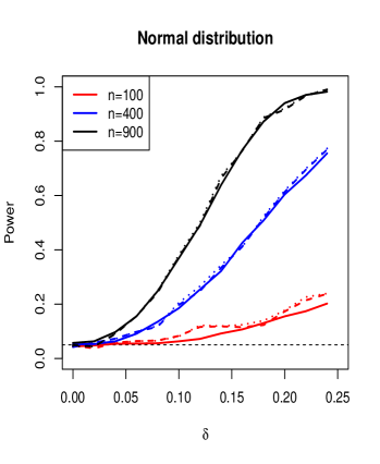
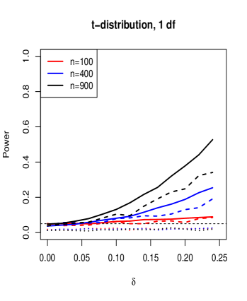
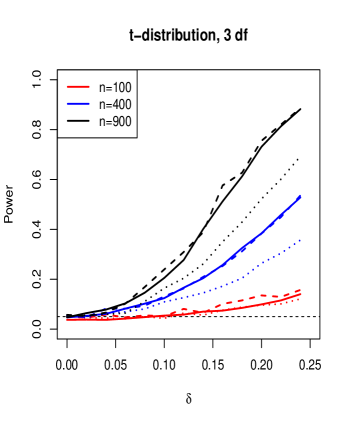
Figure 2: Empirical powers of two-sample location tests based on the Wilcoxon center-outward rank statistic (solid line), the Wilcoxon elliptical rank statistic (dashed line), and Hotelling’s two-sample test (dotted line), as functions of the shift $\delta$ under bivariate normal and elliptical Student (1 and 3 degrees of freedom) error densities; sample sizes $n_{1}=n_{2}=50$ (red), $200$ (blue), and $450$ (black).

Figure 2 displays the empirical power curves for the elliptical distributions (a) and (b). The results for the normal distribution are very similar for the three tests: rank-based tests (Wilcoxon scores), thus, are no less powerful than the optimal Hotelling test. As expected, Hotelling crashes under the $t_{1}$ distribution, while the Wilcoxon elliptical test, although based on the sample covariance matrix, performs surprisingly well (the robustness of ranks offsets infinite variance). The tests based on $\stackunder[1pt]{Q}{\scriptscriptstyle\thicksim}^{(n)\,\text{\rm{ell}}}_{\text{\tiny Wilcoxon}}$ and $\stackunder[1pt]{Q}{\scriptscriptstyle\thicksim}^{(n){\scriptscriptstyle\pm}}_{\text{\tiny Wilcoxon}}\vspace{0.2mm}$ both outperform Hotelling also for the $t$-distribution with 3 degrees of freedom. The conclusion is that center-outward rank tests perform equally well as elliptical rank tests under elliptical densities.

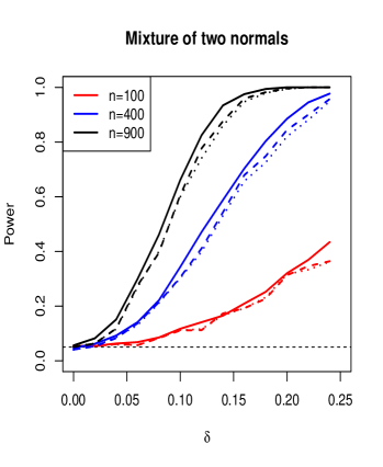
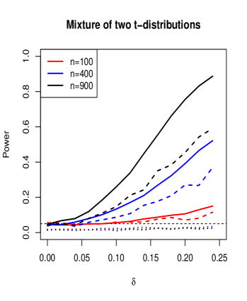
Figure 3: Empirical powers of two-sample location tests based on the Wilcoxon center-outward rank statistic (solid line), the Wilcoxon elliptical rank test statistic (dashed line), and Hotelling’s two-sample test (dotted line), as functions of the shift $\delta$, for the mixtures of two normal (left panel) and two $t_{1}$ error densities (right panel), respectively; sample sizes $n_{1}=n_{2}=50$ (red), $200$ (blue), and $450$ (black).

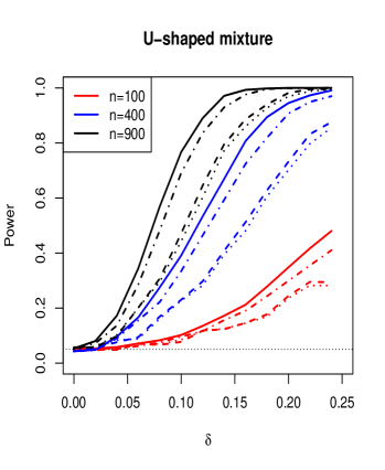
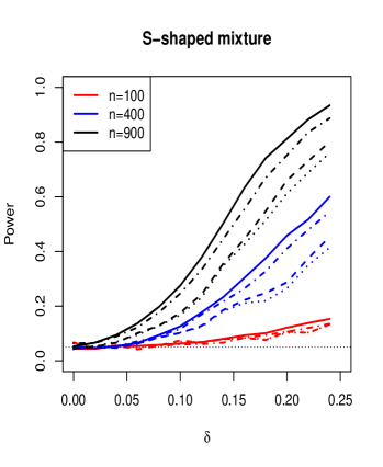
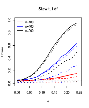
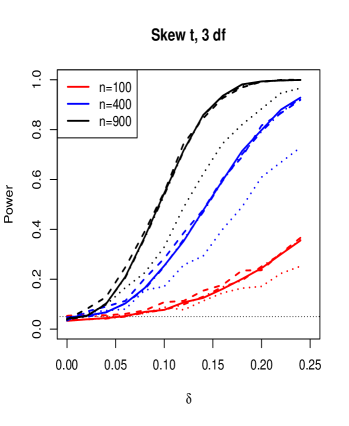
Figure 4: Empirical powers of two-sample location tests based on the Wilcoxon center-outward rank statistic (solid line), the Wilcoxon center-outward rank statistic computed from linearly sphericized residuals (dot-dashed line), the Wilcoxon elliptical rank test statistic (dashed line), and Hotelling’s two-sample test (dotted line), as functions of the shift $\delta$ for the ”U-shaped” (upper left panel) and the ”S-shaped” (upper right panel) mixtures of three normal error densities, and skew-$t$ error densities with $\nu=1.1$ (bottom left panel) and $\nu=3$ (bottom right panel) degrees of freedom, respectively; sample sizes $n_{1}=n_{2}=50$ (red), $200$ (blue), and $450$ (black).

The remaining distributions (c)–(g) are non-elliptical ones. Results for the mixtures (c) and (d) are shown in Figure 3. For the mixture (c) of two normals, the results obtained for the three tests are still quite similar, but the center-outward rank test based on $\stackunder[1pt]{Q}{\scriptscriptstyle\thicksim}^{(n){\scriptscriptstyle\pm}}_{\text{\tiny Wilcoxon}}$, in general, yields the largest power. For the mixture (d) of two $t_{1}$ (Cauchy) distributions, the Hotelling test fails miserably and the center-outward rank test very clearly outperforms the elliptical rank test for all sample sizes. Figure 4 provides the results for the mixtures (e)–(f) and the skew-$t$-distribution (g), respectively. The power curve for the test statistic $\stackunder[1pt]{Q}{\scriptscriptstyle\thicksim}^{(n){\scriptscriptstyle\pm}}_{\text{\tiny Wilcoxon}}$ computed from the linearly sphericized residuals (using the sample mean and the sample covariance matrix as estimators of location and scatter) is added as a dot-dashed line. In all these plots, the center-outward rank test statistic leads to the largest power. Note that the linear sphericization of the residuals, which makes the test affine-invariant, may noticeably deteriorate the power (see the discussion in Section 6.3 and Appendix A.6).

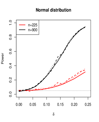
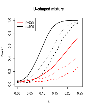
Figure 5: Empirical powers of MANOVA tests based on the Wilcoxon center-outward rank statistic (solid line), the Wilcoxon elliptical rank test statistic (dashed line), Pillai’s test (dotted line), and Roy’s test (dashed-dotted line) as functions of the shift $\delta$, for the normal distribution (left panel) and the U-shaped mixture of three normals (right panel); the sample sizes are $n_{1}=n_{2}=n_{3}=75$ (red) and $300$ (black).

7.2 One-way MANOVA, $d=2$

The performance of center-outward rank tests is very briefly studied here for one-way MANOVA with $K=3$ groups, still for $d=2$. Two random samples were generated from the distribution (a) (Gaussian) or (e) (U-shaped mixture of three Gaussians), as described in Section 7.1, and the third sample was drawn from the same distribution shifted by the vector $(\delta,\delta)^{\prime}$ for $\delta\in[0.00,0.24]$. A balanced design with groups of size $n_{1}=n_{2}=n_{3}=75$ (hence $n=225$) and $n_{1}=n_{2}=n_{3}=300$ (hence $n=900$) was considered. For $n=225$, the grid $\mathfrak{G}_{n}$ is constructed with $n_{R}=n_{S}=15$; for $n=900$, we set $n_{R}=n_{S}=30$. As in Section 7.1, the results are presented for the Wilcoxon scores $J(r)=r$ only—other choices lead to very similar conclusions.

Rejection frequencies are plotted in Figure 5 for the center-outward rank test based on $\stackunder[1pt]{Q}{\scriptscriptstyle\thicksim}^{(n){\scriptscriptstyle\pm}}_{\text{\tiny Wilcoxon}}$ (solid line), the elliptical rank test statistic $\stackunder[1pt]{Q}{\scriptscriptstyle\thicksim}^{(n)\,\text{\rm{ell}}}_{\text{\tiny Wilcoxon}}$ (dashed line), the Pillai trace test based on an approximate F-distribution (dotted line), and the Roy test (dashed-dotted line); see the Supplementary Material for implementation. Under normal density, all the tests perform very similarly. For the non-elliptical mixture distribution, however, the center-outward rank test achieves sizeably larger power than all other ones. Further simulations yielding, in dimension $d=6$, similar conclusions, are provided in Appendix A.7.

7.3 An empirical illustration

The practical value of the center-outward rank tests developed in the previous sections is illustrated with the following archeological application where classical methods fail to detect any treatment effect. The data consist of $n=126$ measurements of MgO (Magnesium oxide), P₂O₅ (Phosphorus pentoxide), CoO (Cobalt monoxide), and Sb₂O₃ (Antimony trioxide) (dimension $d=4$, thus) in natron glass vessels excavated from three Syro-Palestinian sites in present-day Israel: Apollonia ($n_{1}=54$ observations), Bet Eli’ezer ($n_{2}=17$ observations), and Egypt ($n_{3}=55$ observations); a fourth site only has two observations and was dropped from the analysis. This dataset has been originally analyzed by Phelps et al., (2016) with the objective of detecting possible differences among the three sites. Bivariate plots of these four variables are shown in Figure 6, where one can observe that the marginal distributions of CoO, and Sb₂O₃ exhibit heavy tails and are very far from normal, and their joint distribution far from elliptically symmetric. A traditional (pseudo-Gaussian) test here is Pillai’s trace test reducing, in the two-sample case, to Hotelling’s classical $T$-square test.

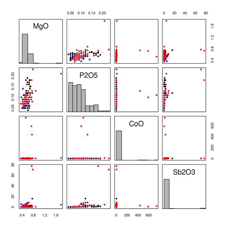
Figure 6: The content of MgO, P₂O₅, CoO, and Sb₂O₃ in natron glass vessels from Appolonia (circles), Bet Eli’ezer (triangles), and Egypt (squares).

First, all the two-dimensional data subsets corresponding to the bivariate plots in Figure 6 were analyzed (six bivariate MANOVA models, thus). Pillai’s test yields non-significant $p$-values for all combinations, see Table 2. But the center-outward tests we are proposing in this paper do detect significant differences between the three groups whenever the variable CoO is included in the analysis. Two versions of the center-outward ranks and signs are considered in Table 2 below (c-o tests I and II, respectively; these two versions correspond to two choices of the grid $\mathfrak{G}_{n}$, with either $n_{S}=7$ and $n_{R}=18$ or $n_{S}=18$ and $n_{R}=7$—see Section 2.2 for an explanation).

		Pillai’s test	Roy’s test	c-o test I	c-o test II
MgO	P2O5	0.3547	0.3568	0.3817	0.0946
MgO	CoO	0.1217	0.1592	0.0000	0.0000
MgO	Sb2O3	0.2268	0.3744	0.1865	0.3239
P2O5	CoO	0.1491	0.2747	0.0000	0.0000
P2O5	Sb2O3	0.1957	0.3379	0.0569	0.2770
CoO	Sb2O3	0.1453	0.1110	0.0000	0.0000

Table 2: $p$-values for the bivariate MANOVA Pillai trace and Wilcoxon center-outward rank tests based on $n_{R}=7$, $n_{S}=18$ (c-o test I) and $n_{R}=18$, $n_{S}=7$ (c-o test II), respectively.

Inspection of Table 2 reveals that, unlike Pillai’s trace, the Wilcoxon center-outward rank tests (c-o I and II) reject the null hypothesis at significance level $\alpha=0.05$. As for the Wilcoxon tests based on elliptical ranks (based on the sample covariance function), they yield highly non-significant $p$-values for all couples of variables; the corresponding results are not presented here. Next, the MANOVA comparison is conducted for the full $4$-dimensional dataset. Pillai’s and Roy’s $p$-values are $0.1553$ and $0.2765$, respectively: no difference detected among the three groups, thus, at level $\alpha=0.05$. In sharp contrast, the Wilcoxon center-outward rank test (with $n_{R}=7$ and $n_{S}=18$) yields a $p$-value $10^{-15}$, which is highly significant. The elliptical Wilcoxon rank test (based on the sample covariance matrix), on the other hand, with $p$-value $0.5827$, also fails to detect anything at any level $\alpha\leq 0.5$.

This, according to archeological sources, might lead to revising some of the conclusions made by Phelps et al., (2016) on Middle-East economic exchanges between Egypt and Syro-Palestine in the Byzantine-Islamic transition period.

8 Conclusion and perspectives

Classical multivariate analysis methods, which are daily practice in a number of applied domains, remain deeply marked by Gaussian and elliptical assumptions. In particular, no distribution-free approach is available so far for hypothesis testing in multiple-output regression models, which include the fundamental two-sample and MANOVA models—except for the elliptical or Mahalanobis rank tests developed in Hallin and Paindaveine, (2005) which, however, require the strong assumption of elliptic symmetry—an assumption which is unlikely to hold in most applications. Based on the recent concept of center-outward ranks and signs, this paper proposes the first efficient fully distribution-free tests of the hypothesis of no treatment effect in that multiple-output context, thereby extending to the multivariate case the classical Hájek approach to univariate rank-based inference (Hájek and Šidák, , 1967). Simulations and an empirical example demonstrate the excellent performance of the method. This lays the theoretical bases (asymptotic representation and asymptotic normality results for linear center-outward rank statistics) and theoretical guidelines (Hájek projection of LAN central sequences) for the development of a complete toolbox of distribution-free methods for multivariate analysis.

References

• Beirlant et al., (2020) Beirlant, J., Buitendag, S., del Barrio, E., and Hallin, M. (2020). Center-outward quantiles and the measurement of multivariate risk. Insurance: Mathematics and Economics, 95:79–100.
• Boeckel et al., (2018) Boeckel, M., Spokoiny, V., and Suvorikova, A. L. (2018). Multivariate Brenier cumulative distribution functions and their application to non-parametric testing. Available at arXiv:1809.04090v1.
• Chernoff and Savage, (1958) Chernoff, H. and Savage, I. R. (1958). Asymptotic normality and efficiency of certain nonparametric test statistics. The Annals of Mathematical Statistics, 29(4):972 – 994.
• Chernozhukov et al., (2017) Chernozhukov, V., Galichon, A., Hallin, M., and Henry, M. (2017). Monge-Kantorovich depth, quantiles, ranks, and signs. The Annals of Statistics, 45:223–256.
• De Valk and Segers, (2018) De Valk, C. and Segers, J. (2018). Stability and tail limits of transport-based quantile contours. Available at arXiv:1811.12061.
• Deb et al., (2021) Deb, N., Bhattacharya, B. B., and Sen, B. (2021). Efficiency lower bounds for distribution-free Hotelling-type two-sample tests based on optimal transport. Available at arXiv:2104.01986.
• Deb and Sen, (2019) Deb, N. and Sen, B. (2019). Multivariate rank-based distribution-free nonparametric testing using measure transportation. Journal of the American Statistical Association, to appear.
• del Barrio et al., (2020) del Barrio, E., González-Sanz, A., and Hallin, M. (2020). A note on the regularity of optimal-transport-based center-outward distribution and quantile functions. Journal of Multivariate Analysis, 180(C):S0047259X20302529.
• Dodge and Jurečková, (2000) Dodge, Y. and Jurečková, J. (2000). Adaptive Regression. Springer, New York.
• Dua and Graff, (2017) Dua, D. and Graff, C. (2017). UCI machine learning repository.
• Fang et al., (2017) Fang, K. T., Kotz, S., and Ng, K. W. (2017). Symmetric Multivariate and Related Distributions. Chapman & Hall/CRC Monographs on Statistics & Applied Probability. Taylor & Francis, Boca Raton.
• Figalli, (2018) Figalli, A. (2018). On the continuity of center-outward distribution and quantile functions. Nonlinear Analysis. Theory, Methods & Applications. Series A: Theory and Methods, 177:413–421.
• Garel and Hallin, (1995) Garel, B. and Hallin, M. (1995). Local asymptotic normality of multivariate ARMA processes with a linear trend. Annals of the Institute of Statistical Mathematics, 47:551–579.
• Ghosal and Sen, (2019) Ghosal, P. and Sen, B. (2019). Multivariate ranks and quantiles using optimal transportation and applications to goodness-of-fit testing. Available at arXiv:1905.05340.
• Hájek and Šidák, (1967) Hájek, J. and Šidák, Z. (1967). Theory of Rank Test. Academic Press, New York.
• Hallin, (1994) Hallin, M. (1994). On the Pitman non-admissibility of correlogram-based methods. Journal of Time Series Analysis, 15(6):607–611.
• Hallin, (2017) Hallin, M. (2017). On distribution and quantile functions, ranks, and signs in $\mathbb{R}^{d}$: a measure transportation approach. Available at ideas.repec.org/p/eca/wpaper/2013-258262.html.
• Hallin, (2022) Hallin, M. (2022). Measure transportation and statistical decision theory. Annual Review of Statistics and its Application, 9.
• (19) Hallin, M., del Barrio, T., Cuesta-Albertos, J., and Matrán, C. (2021a). On distribution and quantile functions, ranks, and signs in $\mathbb{R}^{d}$: a measure transportation approach. The Annals of Statistics, 49:1139–1165.
• (20) Hallin, M., Hlubinka, D., and Šárka Hudecová (2020a). Fully distribution-free center-outward rank tests for multiple-output regression and MANOVA. Available at arXiv:2007.15496.
• Hallin et al., (1985) Hallin, M., Ingenbleek, J. F., and Puri, M. L. (1985). Linear serial rank tests for randomness against ARMA alternatives. The Annals of Statistics, 13:1156–1181.
• Hallin et al., (1989) Hallin, M., Ingenbleek, J. F., and Puri, M. L. (1989). Asymptotically most powerful rank tests for multivariate randomness against serial dependence. Journal of Multivariate Analysis, 30:34–71.
• (23) Hallin, M., La Vecchia, D., and Liu, H. (2020b). Rank-based testing for semiparametric VAR models: a measure transportation approach. Available at arXiv:2011.06062.
• (24) Hallin, M., La Vecchia, D., and Liu, H. (2021b). Center-outward R-estimation for semiparametric VARMA models. Journal of the American Statistical Association, to appear.
• Hallin and Mordant, (2021) Hallin, M. and Mordant, G. (2021). On the finite-sample performance of measure transportation-based multivariate rank tests. Available at arXiv:2111.04705.
• (26) Hallin, M. and Paindaveine, D. (2002a). Optimal procedures based on interdirections and pseudo-Mahalanobis ranks for testing multivariate elliptic white noise against ARMA dependence. Bernoulli, 8:787–815.
• (27) Hallin, M. and Paindaveine, D. (2002b). Optimal tests for multivariate location based on interdirections and pseudo-Mahalanobis ranks. The Annals of Statistics, 30:1103–1133.
• Hallin and Paindaveine, (2004) Hallin, M. and Paindaveine, D. (2004). Rank-based optimal tests of the adequacy of an elliptic VARMA model. The Annals of Statistics, 32(6):2642–2678.
• Hallin and Paindaveine, (2005) Hallin, M. and Paindaveine, D. (2005). Affine-invariant aligned rank tests for multivariate general linear models with VARMA errors. Journal of Multivariate Analysis, 93:122–163.
• Hallin and Puri, (1994) Hallin, M. and Puri, M. L. (1994). Aligned rank tests for linear models with autocorrelated errors. Journal of Multivariate Analysis, 50:175–237.
• Hornik, (2005) Hornik, K. (2005). A CLUE for CLUster Ensembles. Journal of Statistical Software, 14(12).
• Judd, (1998) Judd, K. L. (1998). Numerical Methods in Economics. MIT Press, Cambridge, MA.
• Koul and Saleh, (1993) Koul, H. L. and Saleh, A. K. M. (1993). R-estimation of the parameters of autoregressive AR($p$) models. The Annals of Statistics, 21:534–551.
• LeCam, (1986) LeCam, L. (1986). Asymptotic Methods in Statistical Decision Theory. Springer, New York.
• Lehmann and Romano, (2005) Lehmann, E. L. and Romano, J. P. (2005). Testing Statistical Hypotheses, 3rd Edition. Springer, New York.
• Lind and Roussas, (1972) Lind, B. and Roussas, G. (1972). A remark on quadratic mean differentiability. The Annals of Mathematical Statistics, 43:1030–1034.
• Liu, (1992) Liu, R. Y. (1992). Data depth and multivariate rank tests. In Dodge, Y., editor, $L^{1}$ Statistics and Related Methods, pages 279–294. North-Holland, Amsterdam.
• Liu and Singh, (1993) Liu, R. Y. and Singh, K. (1993). A quality index based on data depth and multivariate rank tests. Journal of the American Statistical Association, 88:257–260.
• McCann, (1995) McCann, R. J. (1995). Existence and uniqueness of monotone measure-preserving maps. Duke Mathematical Journal, 80:309–324.
• Mérigot, (2011) Mérigot, Q. (2011). A multiscale approach to optimal transport. In Computer Graphics Forum, volume 30, pages 1583–1592. Wiley Online Library.
• Niederreiter, (1992) Niederreiter, H. (1992). Random Number Generation and Quasi-Monte Carlo Methods, volume 63 of CBMS-NSF Regional Conference Series in Applied Mathematics. SIAM Society for Industrial and Applied Mathematics, Philadelphia, PA.
• Oja, (1999) Oja, H. (1999). Affine invariant multivariate sign and rank tests and corresponding estimates: a review. Scandinavian Journal of Statistics, 26:319–343.
• Oja, (2010) Oja, H. (2010). Multivariate Nonparametric Methods with R: an approach based on spatial signs and ranks. Springer, New York.
• Peyré and Cuturi, (2019) Peyré, G. and Cuturi, M. (2019). Computational optimal transport. Foundations and Trends$\circledR$ in Machine Learning, 11(5–6):355–607.
• Phelps et al., (2016) Phelps, M., Freestone, I. C., Gorin-Rosen, Y., and Gratuze, B. (2016). Natron glass production and supply in the late antique and early medieval Near East: The effect of the Byzantine-Islamic transition. Journal of Archaeological Science, pages 57–71.
• Puri and Sen, (1971) Puri, M. L. and Sen, P. K. (1971). Nonparametric Methods in Multivariate Analysis. Wiley, New York.
• Puri and Sen, (1985) Puri, M. L. and Sen, P. K. (1985). Nonparametric Methods in General Linear Models. Wiley, New York.
• R Core Team, (2021) R Core Team (2021). R: A Language and Environment for Statistical Computing. R Foundation for Statistical Computing, Vienna, Austria.
• Randles and Wolfe, (1979) Randles, R. and Wolfe, D. (1979). Introduction to the Theory of Nonparametric Statistics. Wiley, New York.
• Santner et al., (2003) Santner, T. J., Williams, B. J., and Notz, W. I. (2003). The Design and Analysis of Computer Experiments. Springer-Verlag, New York.
• (51) Shi, H., Drton, M., Hallin, M., and Han, F. (2021a). Center-outward sign- and rank-based quadrant, Spearman, and Kendall tests for multivariate independence. Available at arXiv:2111.15567.
• (52) Shi, H., Drton, M., and Han, F. (2021b). Distribution-free consistent independence tests via center-outward ranks and signs. Journal of the American Statistical Association, to appear.
• (53) Shi, H., Hallin, M., Drton, M., and Han, F. (2021c). On universally consistent and fully distribution-free rank tests of vector independence. The Annals of Statistics, to appear.
• Street et al., (1993) Street, W. N., Wolberg, W. H., and Mangasarian, O. L. (1993). Nuclear feature extraction for breast tumor diagnosis. In Acharya, R. S. and Goldgof, D. B., editors, Biomedical Image Processing and Biomedical Visualization, volume 1905, pages 861 – 870. International Society for Optics and Photonics, SPIE.
• Tyler, (1987) Tyler, D. (1987). A distribution-free M-estimator of multivariate scatter. The Annals of Statistics, 15:234–251.
• Zuo and He, (2006) Zuo, Y. and He, X. (2006). On limiting distributions of multivariate depth-based rank sum statistics and related tests. The Annals of Statistics, 34:2879–2896.