Deep neural network approximations for the stable manifolds of the Hamilton-Jacobi equations

Abstract.

As the Riccati equation for control of linear systems, the Hamilton-Jacobi-Bellman (HJB) equations play a fundamental role for optimal control of nonlinear systems. For infinite-horizon control problem, the optimal control can be represented by the stable manifold of the characteristic Hamiltonian system of HJB equation. In this paper, we study the deep neural network (NN) semiglobal approximation of the stable manifold. Our main contribution includes twofold: firstly, from the mathematical point of view, we theoretically prove that if an approximation is sufficiently close to the exact stable manifold of the HJB equation, then the corresponding control derived from this approximation stabilizes the system and is nearly optimal. Secondly, based on the theoretical result, we propose a deep learning approach to approximate the stable manifold and compute optimal feedback control numerically. Our algorithm is based on the geometric features of the stable manifold and relies on adaptive data generation through finding trajectories randomly within the stable manifold. To achieve this, we solve two-point boundary value problems (BVPs) locally near the equilibrium and extend the local solutions using initial value problems (IVPs) for the characteristic Hamiltonian system. We randomly choose a number of samples along each trajectory, and adaptively select additional samples near points with large errors from the previous round of training. Our algorithm is causality-free basically, hence it has the potential to apply to a wide range of high-dimensional nonlinear systems. We demonstrate the effectiveness of our method through two examples: stabilizing the Reaction Wheel Pendulums and controlling the parabolic Allen-Cahn equation.

1. Introduction

1.1. Motivation and literature review

It is well known that the theory and computation tools for the Riccati equation were well developed and have been applied widely to various fields. In contrast, Hamilton-Jacobi-Bellman (HJB) equations present greater challenges since in general they are nonlinear first-order partial differential equations, and finding analytical solutions is infeasible. As a result, research on HJB equations is more complicated and requires advanced computation tools and techniques. In this paper, we focus on the stationary HJB equations which are related to infinite horizon optimal control and $H^{\infty}$ control problems. The stabilizing solutions of the stationary HJB equations correspond to the stable manifolds of the characteristic Hamiltonian systems at certain equilibriums (cf. e.g. [48, 43]). Once the stable manifold is obtained, the optimal control can be represented directly by the stable manifold ([43]) without using the gradient of the solution of the HJB equation. This approach can be considered as a natural generalization of LQ theory to nonlinear systems.

Computing stable manifolds for Hamilton-Jacobi equations is generally challenging. In [43], the authors proposed an iterative procedure for approximating the exact trajectories of the characteristic Hamiltonian system on the stable manifold. Although this method has produced promising feedback controls for certain initial conditions or in the vicinity of nominal trajectories, as demonstrated in [42, 21, 20], it can become time-consuming when attempting to compute feedback controls for more general initial conditions or for high-dimensional state systems.

Numerous works have been devoted to numerically solving Hamilton-Jacobi equations, motivated by various applications, as in [7, 35, 6, 15, 26, 24, 4, 32, 36, 23] and the references therein. However, these existing methods may suffer from one or more of the following limitations, as pointed out in [33]: heavy computational cost for higher-dimensional systems, difficulty in estimating solution accuracy for general systems, solution obtained only in a small neighborhood of a fixed point or nominal trajectory, and requirement for special structures in the nonlinear terms of the system.

Recently, various deep learning methods have been developed for efficiently solving Hamilton-Jacobi equations in large domains of high dimensions, using grid-free sampling. For instance, [47, 45] propose to seek neural network (NN) approximate solutions of the Hamilton-Jacobi equation by minimizing the residual of the PDE and boundary conditions on a set of randomly sampled collocation points with a certain size. The papers [18] and [39] propose deep learning methods for solving PDEs, including HJB equations, by reformulating the PDEs as stochastic differential equations. [31] establishes a theory for searching neural networks to approximate optimal feedback laws on suitable functional spaces. Moreover, [33, 27] propose a causality-free data-driven deep learning algorithm for solving HJB equations, making NN training more effective through adaptive data generation. This data generation relies on solving a two-point BVP of the characteristic system of the HJB equation, also known as Pontryagin’s Maximum Principle. These approaches are grid-free and can be applied to high-dimensional problems.

1.2. Contributions

The aim of the paper is to seek deep NN semiglobal approximations of stable manifolds. The main contributions are as follows.

The first main contribution of this paper is to provide theoretical proof that, under appropriate accuracy assumptions, the control derived from the neural network (NN) approximation of the stable manifold stabilizes the system and is sufficiently close to the exact optimal control. The related results are presented in Theorems 3.2 and Corollary 3.2 in Section 3. The proof involves a meticulous asymptotic analysis of the closed loop trajectories from the controller generated by the NN approximation.

It is important to note that our approach differs from those focused on solving the Hamilton-Jacobi-Bellman (HJB) equations, such as those discussed in [45, 33]. Our method is based on the stable manifold, an intrinsic geometric property of the HJB equation. With our framework, we can ensure the stability of the closed loop from the controller generated by the trained NN satisfying certain accuracy. Relative to the literature on this topic, there are few theoretical results. In empirical algorithms, the ‘equilibrium’ of the closed loop system from the NN may become unstable or disappear as time goes to infinity, as shown in [34]. Moreover, our method is different from that in [34], which devises certain architectures for approximate NN to stabilize the system.

The second main contribution of this paper is the development of an algorithm for generating deep NN approximations of the stable manifold, which is based on the theoretical results presented above. One of the crucial aspects of this algorithm is the selection of the loss function for the NN. To achieve this, we utilize a composite loss function that incorporates the maximum error, the mean error of the NN from the exact stable manifold on the sample set, and the error between the derivative of the NN at the origin and the stabilizing solution of the Riccati equation (as shown in equation (4.3)).

Another crucial issue is adaptive data generation by solving the characteristic Hamiltonian systems which is motivated by [33]. Procedure of algorithm is as follows. Firstly, we solve a small set of trajectories in the stable manifold by using a two-point boundary value problem (BVP) for the characteristic Hamiltonian system. The boundary conditions are randomly chosen within a small sphere centered at $0$, as shown in equation (2.30)-(2.37) . These trajectories are then extended by solving the initial value problem (IVP) of the characteristic Hamiltonian system. Next, we randomly select a specified number of samples on these trajectories and denote this set of samples as $\mathcal{D}_{1}$. Secondly, we train a deep NN approximation of the stable manifold on $\mathcal{D}_{1}$. Thirdly, we select samples in $\mathcal{D}_{1}$ with large errors, randomly choose a certain number of samples around these points as the boundary conditions, and solve the BVP to generate a larger sample set $\mathcal{D}_{2}\supset\mathcal{D}_{1}$. Finally, we train the neural network again on $\mathcal{D}_{2}$ to obtain a more accurate NN approximation of the stable manifold. We repeat this process until the desired accuracy is achieved. This approach is causality-free and does not depend on discretizing the space, making it suitable for high-dimensional problems. Causality-free algorithms have proven successful in various applications, such as those discussed in [28, 30, 29, 49, 12, 18].

In comparison to [45, 33], our algorithm trains NN to approximate the stable manifold without requiring the computation of the gradient of the NN approximate solution of the HJB equation, thereby reducing computation costs. Moreover, our algorithm has three key ingredients.

Firstly, we solve the two-point BVP in the neighborhood of the origin and extend the local trajectories to larger ones by solving the initial value problem on a negative time interval. This approach has several advantages, including better convergence rates for the two-point BVP solver since the boundary condition is restricted near the origin, and more flexibility in solving the IVP due to the availability of various numerical methods such as Runge-Kutta, symplectic integrators, and variational integrators.

Secondly, we select a certain number of samples on each trajectory according to an exponential distribution near the equilibrium with respect to time $t>0$ and a uniform distribution away from the equilibrium with respect to the negative time interval. This technique reduces the number of trajectories that must be found and generates samples using the geometric feature of the stable manifold, making the training of the NN approximation more efficient.

Thirdly, we rescale the model at the beginning of the algorithm to enhance the convergence of the BVP solver and make the NN training more effective.

It is worth noting that in [43, 42], the algorithms are based on an iterative procedure in a small neighborhood of the equilibrium, which is difficult to estimate accurately. In contrast, our algorithm directly solves two-point BVP with a boundary point on a relatively larger sphere and extends the local trajectories by solving IVP. The convergence rate of the BVP solver can be flexibly controlled by testing on a small set of randomly chosen samples. Additionally, we use deep NNs to approximate the stable manifold. Compared to traditional approximations such as polynomials ([10]), the parameters of deep NN can be updated more flexibly by adding adaptive samples to the training set to improve accuracy.

To demonstrate the effectiveness of our method, we present two applications. Firstly, we use our algorithm to compute the approximate optimal feedback controls for swinging up and stabilizing the Reaction Wheel Pendulum. This highly nonlinear problem is widely regarded as a benchmark for testing nonlinear control methods. With the proposed method, we can efficiently compute feedback control for points in a semi-global domain. Secondly, we apply our algorithm to the optimal control of the parabolic Allen-Cahn equation. We approximate this nonlinear infinite-dimensional control problem by a high-dimensional control problem (e.g., 30-dimensional in our implementation). The NN training for both problems is performed on an ordinary laptop, demonstrating the practicality and efficiency of our approach. In particular, by simulation, the time to generate the control signal from the trained NN takes less than one millisecond on average. This implies that our method enables real-time control in practice.

1.3. Organization

The paper is structured as follows. In Section 2, we provide a brief overview of the stable manifolds of HJB equations. Section 3 presents a rigorous asymptotic analysis for the NN approximation of the stable manifold. Section 4 outlines the details of the deep learning algorithm. Section 5 focuses on the implementation of our algorithm for swinging up and stabilizing the Reaction Wheel Pendulum. Section 6 discusses the application of our method to the optimal control of the parabolic Allen-Cahn equation. In Appendix A, we provide detailed proofs of Theorem 3.2 and Corollary 3.2.

2. The stable manifolds of the HJB equations

In this section, we outline some basic results about the stable manifolds of the HJB equations from nonlinear control theory.

To illustrate the main points of our approach, we restrict our attention to the optimal control problem

$$\dot{x}=f(x)+g(x)u,\quad\mbox{in }\Omega,$$ (2.1)

where $g$ is Lipchitz continuous $n\times m$ matrix-valued function, $u$ is an $m$-dimensional feedback control function of column form, $\Omega\subset\mathbb{R}^{n}$ is a bounded domain with piecewise smooth boundary containing $0$. We assume the instantaneous cost function is given by

$$L(x,u)=q(x)+\frac{1}{2}u^{T}Wu,$$ (2.2)

where $W$ is a positive definite symmetric $m\times m$ matrix, $q(x)\geq 0$ is smooth function. Define the cost functional by

$$J(x,u)=\int_{0}^{+\infty}L(x(t),u(t))dt.$$

The Hamiltonian is $H(x,p)=p^{T}f(x)-\frac{1}{2}p^{T}Rp+q(x)$ and the Hamilton-Jacobi-Bellman equation is

$$H(x,\nabla V)$$

$$= \nabla V^{T}(x)f(x)-\frac{1}{2}\nabla V^{T}(x)R\nabla V(x)+q(x)=0.$$

Here $\nabla V=(\frac{\partial V}{\partial x_{1}},\cdots,\frac{\partial V}{\partial x_{n}})^{T}$ is the gradient of the unknown function $V$ of column form, and

$$R:=g(x)W^{-1}g(x)^{T}.$$ (2.4)

The corresponding feedback control function

$$u(x)=-W^{-1}g(x)^{T}\nabla V(x).$$ (2.5)

Plugging (2.5) into (2.1), we obtain the closed-loop system

$$\dot{x}=f(x)-R(x)\nabla V(x),\quad\mbox{in }\Omega.$$ (2.6)

Throughout the paper, the following assumption will be made:

1. Assume that $f(x)$ and $q(x)$ are $C^{\infty}$ in $\Omega$. For $|x|$ small, $f(x)=Ax+O(|x|^{2})$ and $q(x)=\frac{1}{2}x^{T}Qx+O(|x|^{3})$ with $A\in\mathbb{R}^{n\times n}$, and $Q\in\mathbb{R}^{n\times n}$ is symmetric. Function $g:\Omega\to\mathbb{R}^{n\times m}$ is $C^{\infty}$.

Definition 2.1.

A solution $V$ of (2) is said to be the stabilizing solution if $\nabla V(0)=0$ and $0$ is an asymptotically stable equilibrium of the vector field $f(x)-R(x)\nabla V(x)$.

The characteristic Hamiltonian system of (2) is

$$\left\{\begin{array}[]{l}\dot{x}=f(x)-R(x)p\\ \dot{p}=-(\dfrac{\partial f(x)}{\partial x})^{T}p+\dfrac{1}{2}\dfrac{\partial(p^{T}R(x)p)^{T}}{\partial x}-(\dfrac{\partial q}{\partial x})^{T}.\end{array}\right.$$ (2.9)

Assume $V$ is a stabilizing solution of (2), let

$$\Lambda_{V}:=\left\{(x,p)\,\left|\,p=\nabla V(x)\right.\right\}.$$

It is well known that $\Lambda_{V}$ is invariant under the flow (2.9) (see e.g. [48]). Note that $0$ is an equilibrium of (2.9). The Hamiltonian matrix is given by

$${\rm Ham} := \left(\begin{array}[]{cc}H_{px}(0)&H_{pp}(0)\\ -H_{xx}(0)&-H_{xp}(0)\\ \end{array}\right)$$ (2.12)

$$= \left(\begin{array}[]{cc}A&-R(0)\\ -Q&-A^{T}\\ \end{array}\right).$$ (2.15)

We assume the following condition:

1. ${\rm Ham}$ is hyperbolic and the generalized eigenspace $E_{-}$ for $n$-stable eigenvalues is complementary, that is, $E_{-}\oplus{\rm Im}\left(0,I_{n}\right)^{T}=\mathbb{R}^{2n},$ where $I_{n}$ is the identity matrix of dimension $n$.

We have the following result on stable manifolds obtained by [48].

Theorem 2.1.

Assume that $f,q,R$ satisfy conditions $(C_{1}-C_{2})$. Then the stable manifold $\mathcal{M}$ of (2.9) through $0$ is a smooth submanifold of dimension $n$ in $\mathbb{R}^{2n}$. Moreover, in a neighborhood of $0$, this smooth submanifold can be represented by the graph $\Lambda_{V}$. In particular, there exist $\delta>0$ and $k>0$ such that for all $|x|<\delta$,

$$|p(x)-Px|\leq k|x|^{2},$$

where $P=\frac{\partial^{2}V}{\partial x^{2}}(0)$.

Recall that $P$ is also the stabilizing solution of the Riccati equation ([48])

$$PA+A^{T}P-PR(0)P+Q=0,$$ (2.16)

which can be considered as the linearization of the HJB equation (2) at $0$.

Remark 2.1.

According to the stable manifold theorem established by [48], the tangent space of the stable manifold is given by $\{(x,p)\,|\,p=Px\}$. Since the Hamiltonian matrix satisfies the hyperbolicity assumption, the stable manifold can be locally represented by the graph $\Lambda_{V}$ in a neighborhood of the equilibrium point. See [48] and [43]. Furthermore, it follows that the value function $V$ (i.e., the stabilizing solution of the HJB equation (2)) is $C^{\infty}$ in a neighborhood of the origin in $\mathbb{R}^{n}$.

It is challenging to determine the exact domain where the graph representation of the stable manifold holds due to its close relationship with the regularity of the value function $V$. Specifically, if $V$ is not differentiable at a point $x_{0}$, then the graph representation may not hold in the neighborhood of $x_{0}$. In this paper, we assume that $V$ is a $C^{2}$ function, and the graph representation of the stable manifold is semiglobal, meaning that it holds in a properly large domain containing the origin, where the stable manifold is the graph of $\nabla V$. Further study on the regularity of $V$ is beyond the scope of this work. We refer the interested reader to [8] for a detailed review on this topic.

Remark 2.2.

It is worth noting that although the stable manifold method can be applied to problems that are not linear in control, the notation for such systems can become more cumbersome. Therefore, in this paper, we will focus on control-affine systems of the form (2.1) to emphasize our main point clearly.

In [43], an iterative method for finding trajectories that lie within the stable manifold was proposed (see also [10] for some improvements). However, in this paper, we adopt a different approach based on a two-point BVP to achieve the same goal in a small neighborhood of the origin. Following [43], we set

$$\mathcal{T}=\left(\begin{array}[]{cc}I&S\\ P&PS+I\\ \end{array}\right),$$ (2.19)

where $S$ is the solution of the Lyapunov equation $(A-R(0)P)S+S(A-R(0)P)=R(0)$. Then we have that

$$\mathcal{T}^{-1}{\rm Ham}\mathcal{T}=\left(\begin{array}[]{cc}A-R(0)P&0\\ 0&-(A-R(0)P)^{T}\\ \end{array}\right).$$ (2.22)

Set

$$\left(\begin{array}[]{c}\bar{x}\\ \bar{p}\\ \end{array}\right)=\mathcal{T}^{-1}\left(\begin{array}[]{c}x\\ p\\ \end{array}\right)$$ (2.27)

The characteristic system (2.9) becomes

$$\left\{\begin{array}[]{l}\dot{\bar{x}}=(A-R(0)P)\bar{x}+N_{s}(\bar{x},\bar{p})\\ \dot{\bar{p}}=-(A-R(0)P)^{T}\bar{p}+N_{u}(\bar{x},\bar{p}).\end{array}\right.$$ (2.30)

Here $N_{s}(\bar{x},\bar{p}),N_{u}(\bar{x},\bar{p})$ are the nonlinear term

$$\left(\begin{array}[]{c}f(x)-R(x)p\\ -(\dfrac{\partial f(x)}{\partial x})^{T}p+\dfrac{1}{2}\dfrac{\partial(p^{T}R(x)p)^{T}}{\partial x}-(\dfrac{\partial q}{\partial x})^{T}\\ \end{array}\right)$$ (2.33)

$$~{}~{}~{}~{}~{}~{}~{}~{}~{}~{}~{}~{}~{}~{}~{}~{}~{}~{}~{}~{}~{}~{}~{}~{}~{}~{}~{}~{}~{}~{}~{}~{}~{}~{}-{\rm Ham}\left(\begin{array}[]{c}x\\ p\\ \end{array}\right)$$ (2.36)

with respect to the coordinates $(\bar{x},\bar{p})$. We find the trajectories in the stable manifold by solving (2.30) with boundary condition

$$\bar{x}(0)=\bar{x}_{0},\quad\bar{p}(+\infty)=0.$$ (2.37)

From [43, Theorem 5], we have that

Proposition 2.1.

Suppose conditions $(C_{1})$-$(C_{2})$ hold. For $\bar{x}_{0}$ sufficiently small, there exists unique trajectory of the two-point BVP (2.30)-(2.37) contained in the stable manifold $\mathcal{M}$.

3. Asymptotic analysis of closed-loop system from the NN approximations

This section provides a theoretical analysis of the asymptotic behavior of the closed-loop system, which is obtained using the controller generated from the NN approximation of the stable manifold.

In this paper, we use certain deep NN functions $p^{NN}(\theta,\cdot)$ to approximate the gradient of the value function $V$, denoted by $p(x)$. The universal approximation theorem for neural networks guarantees that we can find an NN approximation $p^{NN}(\theta,\cdot)$ whose graph is sufficiently close to the stable manifold, provided that the number of parameters $\theta$ of the NN is large enough (see [22]). For NNs with one hidden layer (i.e., shallow networks), the number of parameters $\theta$ grows exponentially with the dimension of the state space. This is commonly known as the curse of dimensionality in NN approximation. However, deep NN can overcome this difficulty. A detailed review of this topic can be found in [38]. Thus, we use deep NNs to handle high-dimensional problems in this paper. See Section 4 below.

In this section, we begin by omitting the details of the NN architecture and assuming that, for any given $\varepsilon>0$, there exists an NN function $p^{NN}(\theta,\cdot)$ satisfying the condition

$$|p^{NN}(\theta,x)-p(x)|<\varepsilon\quad\text{for all }x\in\Omega.$$

Here, $p(x)$ denotes the gradient of the value function $V$.

Remark 3.1.

It is important to note that $p^{NN}$ is an approximation of the gradient of the value function $V$, but it may not be the gradient of any function itself. In the following, we will demonstrate mathematically that the approximation $p^{NN}$ can be effectively used for designing optimal feedback controllers under certain natural assumptions.

Hereafter, we assume that $f$, $q$, and $R$ satisfy the conditions outlined in Theorem 2.1, and that $V$ is the stabilizing solution of (2). Since $p(x)=\nabla V(x)$, it follows from equation (2.5) that the optimal control is given by

$$u(x)=-W^{-1}g(x)^{T}p(x).$$ (3.1)

Subsequently, the approximation of the optimal control derived from $p^{NN}(\theta,\cdot)$ is given by

$$u^{NN}(x)=-W^{-1}g(x)^{T}p^{NN}(\theta,x).$$ (3.2)

Let $x(t)$ be the solution of

$$\dot{x}=f(x)-R(x)p(x),\quad x(0)=x_{0}.$$ (3.3)

Assume $x^{NN}(t)$ is the solution of the approximate closed-loop equation

$$\dot{x}=f(x)-R(x)p^{NN}(\theta,x),\quad x(0)=x_{0}.$$ (3.4)

From Assumption $(C_{1})$, it holds that there exist constants $a>0$ and $k>0$ such that for all $|x|<a$,

$$|f(x)-Ax|<k|x|^{2},\quad|g(x)-g(0)|<k|x|,$$

$$|R(x)-R(0)|<k|x|.$$ (3.5)

Since $f,g,R$ are $C^{\infty}$ in $\Omega$, we have that $f,g,R$ are Lipchitz continuous in compact set $\bar{\Omega}$ (the closure of $\Omega$). Moreover, Remark 2.1 yields that $p$ is Lipchitz continuous in $\Omega$. Hereafter, without loss of generality, the Lipschitz constant of $f,g,R,p$ can be chosen as some same constant $L$.

Theorem 3.1.

Let $x(t)$ be the solution of (3.3). There exist constants $C>0$, $b>0$, $\alpha>0$ such that

$$|x(t)|\leq C|x_{0}|e^{-\alpha t},$$ (3.6)

for $t\geq 0$ and $|x_{0}|\leq b$.

Proof.

From Theorem 2.1 and (3), there exists $k_{0}>0$ and $a>0$ such that

$$|f(x)-R(x)p(x)-(Ax-R(0)Px)|\leq k_{0}|x|^{2},\\ \mbox{for all }|x|<a.$$

Recalling that $B:=A-R(0)P$ is Hurwitz, i.e., $B=A-R(0)P$ has all eigenvalues with negative real part, we have the result by [11, Theorem 2.77]. ∎

Remark 3.2.

Since $B=A-R(0)P$ is Hurwitz, there exists a constant $\beta>0$ such that

$$|e^{Bt}x_{0}|\leq|x_{0}|e^{-\beta t}.$$ (3.7)

Hence $\alpha\to\beta^{-}$ as $b\to 0$ in Theorem 3.1. In other words, Theorem 3.1 gives the decay rate of the trajectories of (2.9) in the stable manifold near the equilibrium.

Corollary 3.1.

For any $\varepsilon>0$, by Theorem 3.1, there exists a constant $T_{\varepsilon}>0$ such that

$$|x(t)|<\varepsilon/2,\quad\forall t\geq T_{\varepsilon}.$$ (3.8)

We call $T_{\varepsilon}$ an admissible time of $x$ with respect to $\varepsilon$.

Remark 3.3.

It is possible to obtain a numerical estimation of $T_{\varepsilon}$ in practical scenarios. Additionally, examples in Section 5 and Section 6 indicate that $T_{\varepsilon}$ is typically not large. For instance, in Section 5, from Figure (2) (b) (d), we see that $T_{\varepsilon}$ can be chosen as $5$ since $|x(t)|$ ($t\geq 5$) is almost $0$.

For $x^{NN}$, we have the following asymptotic result whose proof will be included in the Appendix.

Theorem 3.2.

Assume that $p^{NN}(\theta,\cdot)$ satisfies the following conditions:

1. $|p^{NN}(\theta,x)-p(x)|<\delta$ for all $x\in\Omega$, where $\delta>0$ is sufficiently small.

2. $|p^{NN}(\theta,x)-Px|\leq\eta|x|$ for $|x|<\gamma_{0}$, where $\eta>0$ is sufficiently small.

Here, $P$ is the stabilizing solution of Riccati equation (2.16), and $\gamma_{0}>0$ is a fixed constant. Then, the trajectory $x^{NN}(t)$ of the closed-loop system (3.4) generated by the NN controller is sufficiently close to the exact trajectory $x(t)$ of (3.3) with the same initial state $x_{0}\in\Omega$, and $x^{NN}(t)$ decays exponentially as $t\to+\infty$.

Corollary 3.2.

Assume that the conditions of Theorem 3.2 are satisfied. Then the NN generated controller $u^{NN}$ is nearly optimal, i.e., the cost $J(x,u^{NN})$ of controller $u^{NN}$(3.2) is sufficiently close to the cost $J(x,u)$ of exact controller $u$ (3.1).

The proof of this corollary will be given in the Appendix.

Remark 3.4.

The proofs of Theorem 3.2 and Corollary 3.2 in the Appendix provide more precise estimates for the decay rate of $x^{NN}(t)$ (see equation (A.6) below), $|x^{NN}(t)-x(t)|$ (see equation (A.4) below), and $|J(x^{NN},u^{NN})-J(x,u)|$ (see (A.7) below).

4. Algorithm

Section 3 shows that an NN approximation $p^{NN}(\theta,\cdot)$ under certain accuracy can lead to a nearly optimal feedback controller. In this section, we propose a deep learning algorithm based on the theoretical result in Theorem 3.2 to find $p^{NN}(\theta,\cdot)$ that is sufficiently close to $p(\cdot)$ in the sense of conditions (a)-(b) in Theorem 3.2.

4.1. Architecture of the NN

4.1.1. Basic architecture of the NN

To mitigate the curse of dimensionality when numerically solving partial differential equations (PDEs), two crucial challenges should be addressed. The first challenge is related to using NN to approximate functions defined on state spaces with high dimensionality. The complexity of shallow networks, which have only one hidden layer, grows exponentially with the dimension of the state space. In contrast, the complexity of deep NN with a binary tree structure grows only linearly with the dimension of the state space. Readers interested in this topic can refer to [38] for more details. The second challenge is related to the way in which samples are generated. Traditional numerical methods based on grids of the state space suffer from the curse of dimensionality. However, recent progress has been made in using a combination of Monte Carlo methods and deep learning for numerically solving PDE. Interested readers can refer to [17] for a review of this topic.

Although there exist many sophisticated architecture of deep NNs for various purposes, we shall use a neural network architecture introduced by [45] which is similar to long short term memory (LSTM) (see for example [19]). Let $L,\,M\in\mathbb{N}$ be two key hyper-parameters. In the following NN, $L+1$ is the number of hidden layers and $M$ is the number of units in each sub-layer. Let $\sigma:\mathbb{R}^{M}\to\mathbb{R}^{M}$, $\sigma(z)=(\sin(z_{1}),\cdots,\sin(z_{M}))$ be the activation function. The function $\sin(\cdot)$ makes the NN more similar to the Fourier series. Moreover, the derivative of $\sin(\cdot)$, namely $\cos(\cdot)$, has more global support than the derivatives of the traditional activation functions such as sigmoid. Define the NN of the following structure:

$$S^{1}=\sigma(W^{1}x+b^{1}),$$

$$Z^{i}=\sigma(U^{z,i}x+W^{z,i}S^{i}+b^{z,i}),\quad i=1,\cdots,L,$$

$$G^{i}=\sigma(U^{g,i}x+W^{g,i}S^{i}+b^{g,i}),\quad i=1,\cdots,L,$$

$$R^{i}=\sigma(U^{r,i}x+W^{r,i}S^{i}+b^{r,i}),\quad i=1,\cdots,L,$$

$$H^{i}=\sigma(U^{h,i}x+W^{h,i}(S^{i}\odot R^{i})+b^{h,i}),\quad i=1,\cdots,L,$$

$$S^{i+1}=(1-G^{i})\odot H^{i}+Z^{i}\odot S^{i},\quad i=1,\cdots,L,$$

$$p(x,\theta)=WS^{L+1}+b,$$ (4.1)

where $x$ is the input, the output is $p(x,\theta)$, the number of hidden layers is $L+1$, and $\odot$ denotes the Hadamard (element-wise) multiplication. The parameters are given by

$$\theta = \left\{W^{1},b^{1},(U^{z,i},W^{z,i},b^{z,i})_{i=1}^{L},(U^{g,i},W^{g,i},b^{g,i})_{i=1}^{L},\right.$$

$$\left.(U^{r,i},W^{r,i},b^{r,i})_{i=1}^{L},(U^{h,i},W^{h,i},b^{h,i})_{i=1}^{L},W,b\right\},$$

where $W^{1}\in\mathbb{R}^{M\times n}$, $b^{1}\in\mathbb{R}^{M}$, $U^{z,i}\in\mathbb{R}^{M\times n}$, $W^{z,i}\in\mathbb{R}^{M\times M}$, $b^{z,i}\in\mathbb{R}^{M}$, $U^{g,i}\in\mathbb{R}^{M\times n}$, $W^{g,i}\in\mathbb{R}^{M\times M}$, $b^{g,i}\in\mathbb{R}^{M}$, $U^{r,i}\in\mathbb{R}^{M\times n}$, $W^{r,i}\in\mathbb{R}^{M\times M}$, $b^{r,i}\in\mathbb{R}^{M}$, $U^{h,i}\in\mathbb{R}^{M\times n}$, $W^{h,i}\in\mathbb{R}^{M\times M}$, $b^{h,i}\in\mathbb{R}^{M}$, $W^{1\times M}$ and $b\in\mathbb{R}$. For optimization, we use Adam from PyTorch.

In the following, we define an NN of form (4.1.1), $p^{NN}_{o}:=p^{NN}_{o}(\theta;x)$, whose input $x$ and output $p$ are $n$-dimensional.

Remark 4.1.

The architecture of the NN also plays an essential role to avoid the curse of dimensionality. For instance, the complexity of deep NN with binary tree structure to provide approximation with certain accuracy depends linearly on the dimension $n$. See e.g. [38, Theorem 2]. However, the complexity of the NN with just one hidden layer increases exponentially with respect to the dimension $n$ to satisfy certain accuracy. See e.g. [38, Theorem 1]. In this paper, we use a deep NN with architecture of LSTM type. However, we should emphasize that other types of deep NN may also work well. As in [45, 33, 37], to mitigate the curse of dimensionality, we focus the main investigation on control aspect and develop the algorithm based on grdfree method. Further research on the influence of the architecture of deep NN is out the scope of the present work.

4.1.2. Modified NN

In order to find an approximate NN that satisfies condition (b) in Theorem 3.2, we need to modify the architecture of the original NN. Specifically, we define

$$p^{NN}(\theta,x)=p^{NN}_{o}(\theta,x)-p^{NN}_{o}(\theta,0),$$ (4.2)

where $p^{NN}_{o}$ is the output of the original NN architecture given by (4.1.1). With this modification, it is guaranteed that $p^{NN}(\theta,0)=0$, which is a necessary condition for $p^{NN}$ to satisfy condition (b) in Theorem 3.2.

4.1.3. Loss function

To train an NN function $p^{NN}(\theta,\cdot)$ to fit a given dataset $\mathcal{D}=\left\{(x_{i},p_{i})\right\}_{i=1}^{|\mathcal{D}|}$ on $\mathcal{M}$ and ensure that its derivative at $0$ is close to $P$, we define the following loss function for $\nu\in[1,\infty]$:

$$\mathcal{L}^{\nu}(\theta;\mathcal{D}) := \sigma_{1}\left(\frac{1}{|\mathcal{D}|}\sum_{i=1}^{|\mathcal{D}|}\|p_{i}-p^{NN}(\theta;x_{i})\|^{\nu}\right)$$ (4.3)

$$+\sigma_{2}\max_{p_{i}\in\mathcal{D}}|p_{i}-p^{NN}(\theta;x_{i})|$$

$$+\sigma_{3}\left\|\frac{\partial p^{NN}}{\partial x}(\theta,0)-P\right\|,$$

where $|\cdot|$ denotes the standard Euclidean norm in $\mathbb{R}^{n}$, $\|\cdot\|$ is the operator norm of the matrix, $|\mathcal{D}|$ is the number of samples in $\mathcal{D}$, and $\sigma_{i}>0$ for $i=1,2,3$ are weight constants.

To fit our theoretical conclusion in Section 3, the loss function consists of three terms: the first term measures the mean error with exponent $\nu$ between the NN predicted value $p^{NN}(\theta;x_{i})$ and the standard value $p_{i}$ on dataset $\mathcal{D}$; the second term enforces a maximum error constraint, ensuring that the maximum difference between the predicted and observed values is small; and the third term ensures that the derivative of the NN function at $0$ is close to the stabilizing solution $P$ of the Riccati equation (2.16). The weight constants $\sigma_{i}$ control the relative importance of these terms in the overall loss function. Moreover, it is worth noting that the loss function presented here is distinct from that used in [33], which only employs the first term of the loss function (4.3).

Remark 4.2.

When $\nu=2$, the first part of the loss function is the mean square error (MSE), and when $\nu=1$, the first part of the loss function becomes the mean absolute error (MAE).

4.2. The algorithm

In this subsection, we provide a step-by-step procedure for the algorithm used to train an NN to approximate the stable manifold. The outline of the algorithm is as follows.

Algorithm: NN approximation for stable manifold

1. Generate training sample set $\mathcal{D}_{1}$ by BVP solver and

extension IVP. Given training loss tolerance $\varepsilon>0$,

test tolerance $\delta>0$, test/train rate $\gamma\in(0,1)$,

large error sample selecting rate $\zeta\in(0,1)$.

Generate a test sample set $\mathcal{D}_{1}^{\rm val}$ with size $\gamma|\mathcal{D}_{1}|$

using the same method as $\mathcal{D}_{1}$.

2. For $j=1,2,3,\cdots$, do

Train the NN on $\mathcal{D}_{j}$ until $\mathcal{L}^{\nu}(\theta;\mathcal{D}_{j})<\varepsilon$.

if the test error on $\mathcal{D}_{j}^{\rm val}$ is greater than $\delta$, or,

there exist some initial point $x_{0}\in\mathcal{D}_{j}^{\rm val}$ solution

of (3.4) is unstable.

then Select the large error samples of size

$\zeta|\mathcal{D}_{j}|$, generate a sample set $\mathcal{D}_{j}^{+}$ by BVP

solver, set $\mathcal{D}_{j+1}=\mathcal{D}_{j}\cup\mathcal{D}_{j}^{+}$.

Generate a test sample set $\mathcal{D}_{j}^{\rm val,+}$ with size

$\gamma|\mathcal{D}_{j}^{+}|$ using the same method as $\mathcal{D}_{1}^{\rm val}$.

Set $\mathcal{D}_{j+1}^{\rm val}=\mathcal{D}_{j}^{\rm val}\cup\mathcal{D}_{j}^{\rm val,+}$.

End if

End for

We now provide the details of the deep learning algorithm used to find an NN approximation $p^{NN}(\theta,\cdot)$ for the stable manifold. Our algorithm is inspired by [33] and is built on a procedure of adaptively generating data by solving two-point BVPs for the characteristic Hamiltonian system (2.30)-(2.37). The main steps are as follows.

Step 0. Transformation of the model. To enhance the effectiveness of training, we begin by applying a coordinate transformation, such as rescaling, to the characteristic Hamiltonian system (2.9). The necessity of such a transformation is explained in Subsection 4.3.4 below.

Step 1. First selection of trajectories and sampling. We first select some initial points $x$ on the sphere $\partial B_{r}(0)$ using the Monte Carlo sampling method, where $B_{r}(0)\subset\Omega$ is a small ball with radius $r$ centered at the origin. We then use a numerical BVP solver, such as ‘scipy.integrate.solve_bvp’, to solve the BVP (2.30)-(2.37) for each initial point $x$ by taking zero as the initial guess of the solution on a certain number of time nodes. The BVP solver typically converges for $x_{0}\in\partial B_{r}(0)$ with $r$ small. Choosing an appropriate small ball is not a rigorous process, but we can test the convergence rate of the BVP solver for different balls in practice. For example, in Section 5, we choose $B_{0.5}(0)$.

Assume that we obtain $K_{1}$ trajectories $(x_{i}(t),p_{i}(t))$, $t\geq 0$, with $i=1,2,\cdots,K_{1}$ that are contained in the stable manifold. For each trajectory $i$, we then solve the IVP (4.7) on some interval $(T_{-},0]$ ($T_{-}<0$). If the numerical error restrictions are satisfied, then we obtain trajectories that are contained in the stable manifold. We denote the set of $K_{1}$ trajectories by $\mathcal{S}_{1}$. Note that the choice of the sphere $\partial B_{r}(0)$ the interval $(T_{-},0]$ can affect the accuracy and efficiency of the algorithm, and may require some tuning in practice.

On each trajectory $(x_{i}(t),p_{i}(t))$, $t\in(T_{-},\infty)$, we select a certain number of samples for $(T_{-},0]$ and $[0,\infty)$, separately. Specifically, on the positive time interval $[0,\infty)$, we choose $M_{1}^{+}$ samples according to the exponential distribution with respect to time $t$ as explained in (4.13) below. On the negative interval $(T_{-},0]$, we take $M_{1}^{-}$ samples according to the uniform distribution with respect to $t$. Therefore, letting $M_{1}=M_{1}^{+}+M_{1}^{-}$, we now have $N_{1}:=K_{1}\times M_{1}$ samples. Denote the set of those samples contained in the stable manifold by

$$\mathcal{D}_{1}:=\{(x_{i},p_{i})\}_{i=1}^{N_{1}}.$$

Step 2. First NN approximation training. We train an NN of the form (4.1.1) on the data set $\mathcal{D}_{1}$. Specifically, we aim to train the NN so that it satisfies

$$p^{NN}(\theta,x_{i})\approx p_{i},\quad i=1,\cdots,N_{1}.$$

After a certain number of epochs of training, we obtain an NN approximation $p^{NN}(\theta,\cdot)$ with parameters $\theta$ that satisfies the training loss ${\mathcal{L}^{\nu}}(\theta,\mathcal{D}_{1})<\varepsilon$.

Step 3. Adaptive data generation. After the first NN training, we record the absolute errors of the NN approximation on the data set $\mathcal{D}_{1}$ as

$$|p^{NN}(\theta,x_{i})-p_{i}|,\quad i=1,\cdots,N_{1}.$$ (4.4)

We then select the largest $R_{1}=[\mu N_{1}]$ points in $\mathcal{D}_{1}$ according to the errors (4.4), where $[y]$ denotes the integer part of $y$ and $\mu\in(0,1)$ is chosen as in [33, Section 4.1]. Denote the set of these samples by $\mathcal{\hat{D}}_{1}$. We randomly sample $J_{1}$ points $y_{j}\in\Omega$ ($j=1,\cdots,J_{1}$) around $x_{i}$ with $(x_{i},p_{i})\in\mathcal{\hat{D}}_{1}$ according to a certain distribution, such as the normal distribution. We then find solutions of the BVP (2.30)-(2.37) with initial condition $x(0)=y_{j}$ using ‘scipy.integrate.solve_bvp’. Here, we set the initial guess of the solution to be the trajectory, $(x_{i}(t),p_{i}(t))$, $t\in(T_{-},\infty)$, for which $(x_{i},p_{i})$ lies on. We then choose $L_{1}$ samples on each trajectory according to a certain normal distribution with respect to $t$. This process generates more samples near the points whose errors are large. By adding these new samples to $\mathcal{D}_{1}$, we obtain a larger sample set $\mathcal{D}_{2}$.

Step 4. Model refinement. Based on the NN model obtained in Step 2, we continue training the NN function $p^{NN}(\theta,\cdot)$ on the updated data set $\mathcal{D}_{2}$. This refinement of the NN model can improve its accuracy and generalization capabilities.

Step 5. Approximate optimal feedback control. Using the trained NN approximation $p^{NN}(\theta,\cdot)$, we can generate the optimal feedback controller $u^{NN}$ (3.2) and compute the closed-loop trajectories at certain initial conditions $x(0)=x_{0}$ by solving (3.4). For example, see Section 5 and Section 6 below. The computation cost of this procedure is relatively cheap.

Remark 4.3.

We can prove the convergence and effective sample size selection of our algorithm using a progressive batching method, similar to the approach in [33, Section 4]. To enhance the performance and convergence of our algorithm while minimizing computational costs, we utilize a sample size selection scheme based on the sample variances of the training sets $\mathcal{D}_{i}$, where $i=1,2,\cdots$, following the approach proposed in [33, Section 4.1].

Remark 4.4.

The approach in [33] mainly focuses on finding solutions of the HJB equations, specifically the value function $V$ of the optimal control problem. The NN function $V^{NN}(\theta,\cdot)$ approximates the solutions $V$, and $(t_{i},x_{i},V_{x}^{NN}(\theta,x_{i}))$ approximates the sample points $(t_{i},x_{i},p_{i})$, where $p_{i}$ denotes the costate. In that procedure, the gradient $V^{NN}_{x}(\theta,\cdot)$ should be calculated. Additionally, to obtain the optimal feedback control, the gradient should also be computed.

In our algorithm, we focus on computing the stable manifolds, and the NN function $p^{NN}(\theta,\cdot)$ is defined to approximate the points on the stable manifolds. Therefore, the training target is $(x_{i},p^{NN}(\theta,x_{i}))\approx(x_{i},p_{i})$. Although the output of the NN is $n$-dimensional, the computation cost can be reduced since we do not need to calculate the gradients of the NN function.

4.3. Key techniques of the algorithm

To improve the effectiveness of our algorithm, we incorporate several useful techniques as follows.

4.3.1. Solving two-point BVP in a small ball $B_{r}(0)$

To obtain trajectories in the stable manifold, we use ‘scipy.integrate.solve_bvp’ to solve the two-point BVP (2.30)-(2.37) for $x_{0}\in\partial B_{r}(0)$, where $r>0$ is small. Here, $\partial B_{r}(0)$ denotes the sphere centered at $0$ with radius $r$. The details of this BVP solver can be found in [25]. The algorithm implements a 4th-order collocation method with control of residuals similar to [44].

To implement this BVP solver, we need to provide an initial mesh for time and an initial guess for the solution values at each mesh node. The iterative procedure of the BVP solver may diverge if the initial guess is not well chosen. For our problem (2.30)-(2.37), the initial points $x_{0}$ are chosen on the ball $\partial B_{r}(0)$ with small radius $r$, and the initial guess is constantly $0$ on each mesh node. Therefore, the BVP solver converges for most points on this small ball. If $r$ is too large, then the success rate of the BVP solver is not good enough.

To select a proper radius $r$, we use the Monte Carlo method. Specifically, we first choose a small value of $r$, randomly generate some points on the ball $\partial B_{r}(0)$, and then solve the problem (2.30)-(2.37). If the success rate of the BVP solver is $100\%$, then we choose a slightly larger value of $r$. This process continues until the success rate of the BVP solver is not $100\%$. Finally we choose the previous value of $r$ as the radius.

4.3.2. Extension of the local trajectories

Let $(\tilde{x}(t),\tilde{p}(t))$, $t\geq 0$ be a trajectory obtained by the BVP solver. On some interval $(T_{-},0]$, $T_{-}<0$, we solve the following IVP:

$$\left\{\begin{array}[]{l}\dot{x}=f(x)-R(x)p,\\ \dot{p}=-(\dfrac{\partial f(x)}{\partial x})^{T}p+\dfrac{1}{2}\dfrac{\partial(p^{T}R(x)p)^{T}}{\partial x}-(\dfrac{\partial q}{\partial x})^{T},\end{array}\right.$$ (4.7)

$$\mbox{ with }\left\{\begin{array}[]{l}x(0)=\tilde{x}(0),\\ p(0)=\tilde{p}(0).\end{array}\right.$$ (4.10)

To numerically solve this IVP, various methods can be used, such as ‘scipy.integrate.solve_ivp’ with various methods (e.g., ‘RK45‘, ‘Radau‘, etc.), symplectic methods, and variational integrators. Comparing to the BVP solver, the IVP (4.7) is usually much easier to solve. By solving (4.7), we can extend trajectories in the stable manifold. To approximate $T_{-}$, we also use the Monte Carlo method. Specifically, we first choose a value $T_{-}^{0}<0$ and check whether the IVP solver successfully computes the solution for all initial conditions $(\tilde{x}(0),\tilde{p}(0))$ on the interval $(T_{-}^{0},0]$. If the success rate is $100\%$, we then choose a slightly smaller value $T_{-}^{1}<T_{-}^{0}<0$ and repeat the procedure. We continue this process until the IVP solver fails to compute the solution for some initial conditions, and we choose the previous value of $T_{-}$ as the final negative time.

4.3.3. Exponential distribution sampling along trajectories near the equilibrium

Theoretically, every point on the trajectory of (2.30) lies on the stable manifold. Hence, we can pick a certain number of samples along each trajectory. The trajectories on the stable manifold approach the origin exponentially with respect to time $t$, as shown in Theorem 3.1. Therefore, it is reasonable to select samples on the trajectories near the origin according to an exponential distribution:

$$\rho(t)=\left\{\begin{array}[]{cl}\frac{1}{\lambda}e^{-\frac{t}{\lambda}},&t>0,\\ 0,&t\leq 0,\end{array}\right.$$ (4.13)

where $\lambda>0$ is a fixed rate parameter. That is, if we take $t_{0},t_{1},t_{2},\cdots$ from the exponential distribution, then $(x(t_{0}),p(t_{0})),(x(t_{1}),p(t_{1})),(x(t_{2}),p(t_{2})),\cdots$ lie on the stable manifold.

As a special case, suppose $x(t)=x_{0}e^{-\gamma t}$ ($\gamma>0$) with $x_{0}>0$ and $t\in[0,+\infty)$. If we want to select samples on $[0,x_{0}]$ by $t$, then $t$ should be chosen according to the exponential distribution (4.13) with $\lambda^{-1}=\gamma$.

Choosing a different type of distribution may lead to an accumulation of samples around some points. For instance, if we take the uniform distribution on $[0,T]$ for some $T>0$ sufficiently large, then there may be many samples near the origin. The key point is the choice of the parameter $\lambda$. From Theorem 3.1 and Remark 3.2, we see that the decay of $x(t)$ is almost $e^{-\beta t}$ as $t\to+\infty$. In practice, we choose $\lambda=\beta$, where $\beta>0$ is the distance between the set of eigenvalues and the imaginary axis. Using this technique, we can obtain many more samples on the stable manifold by solving fewer two-point BVPs.

Remark 4.5.

Compared to the approach in [33], in our algorithm, we implement BVP solver for $x_{0}$ in a small sphere $\partial B_{r}(0)$ with a constant initial guess. The convergence rate of the BVP solver is good without using the time-march trick as in [33]. Local trajectories are extended by solving the IVP (4.7). We take more samples in each trajectory randomly with certain distributions (e.g., exponential distributions with respect to time $t>0$ and uniform distributions on $(T_{-},0]$), which yields more samples indicating geometric features of the stable manifold. We expand the data set by randomly selecting samples near points with large errors after previous training, improving the accuracy of the NN quickly.

4.3.4. Rescaling

For concrete applications, the original formulation of a model may not be suitable for numerical methods. Hence, modifications should be made at the beginning of the algorithm. From a mathematical point of view, these modifications usually can be chosen as coordinate transformations. In our deep learning algorithm, we use rescaling, which also appears in computational optimal control (see, for example, [41, 40]). Compared to directly solving the HJB equation, such as in [33] and [45], our algorithm is based on the geometric features of the HJB equation. Therefore, it is natural to apply the rescaling of the variables to modify the original model at the beginning of the algorithm.

In (2.9), we apply a rescaling

$$(\hat{x}_{1},\hat{x}_{2},\cdots,\hat{x}_{n})=(\lambda_{1}\bar{x}_{1},\lambda_{2}\bar{x}_{2},\cdots,\lambda_{n}\bar{x}_{n})$$

so that the variables $(\hat{x}_{1},\hat{x}_{2},\cdots,\hat{x}_{n})$ (and their derivatives) have the same orders of magnitude. This modification avoids the stable manifold being too steep in some direction. This modification is essential to the success of the algorithm because it increases the proportion of convergence of the BVP solver and ensures that all variables have the same contribution in the training of the NN approximation. To be more precise, there are two advantages of rescaling in our algorithm. Firstly, after rescaling, the proportion of convergent solutions by the BVP solver increases. As we mentioned, ‘scipy.integrate.solve_bvp’ requires an initial mesh and an initial guess of the solutions. The most convenient guess may be constant at the beginning. Hence if the value and derivative of the exact solution are too large, then the BVP solver may diverge. Secondly, rescaling makes the performance of the NN approximation much better. From the definition of the loss function (4.3), we see that if the orders of magnitude of $x_{1},x_{2},\cdots,x_{n}$ are different, then the weights of some variables in (4.3) are heavy, whereas the weights of others are relatively small and can even be negligible. This may make the training of the NN ineffective. The example in Section 5 below shows that the rescaling technique is essential.

5. Application to the Reaction Wheel Pendulums

The Reaction Wheel Pendulum is a mechanical system that consists of a physical pendulum with a rotating disk (see Figure 1 for a schematic diagram). Nonlinear control researchers have been interested in the swing up and stabilization of various pendulums for the past two decades (see, e.g., [3, 1, 46, 2, 9, 42, 21]). However, existing methods suffer from one or more of the following drawbacks: the controller is not optimal and requires switching between two different laws; the controller may only be valid in a small neighborhood of a certain point; and the computation cost is expensive. For a detailed description of the Reaction Wheel Pendulum device, see [5].

Figure 1. The Reaction Wheel Pendulum

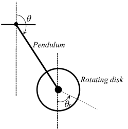
The ideal dynamical system of the Reaction Wheel Pendulum is given by

$$\left\{\begin{array}[]{l}\dot{x}_{1}=x_{2}\\ \dot{x}_{2}=a\sin x_{1}-b_{p}u\\ \dot{x}_{3}=b_{r}u.\\ \end{array}\right.$$ (5.1)

Here $u$ is an input function, $x_{1}=\theta,x_{2}=\dot{\theta},x_{3}=\dot{\theta}_{r}.$ In this implementation, we borrow the parameters of instrument in [5, Page 21]. That is,

$$a=78.4,\,b_{p}=1.08,\,b_{r}=198.$$ (5.2)

For training the NN function $p^{NN}(\theta,\cdot)$, it may be better that $x_{1},x_{2},x_{3}$ and their derivatives have the same orders of magnitude. Hence we redefine the unit of $x_{1},x_{2},x_{3}$. From mathematical point of view, we define a rescaling by

$$\left\{\begin{array}[]{l}x_{1}=\lambda_{1}\bar{x}_{1}\\ x_{2}=\lambda_{2}\bar{x}_{2}\\ x_{3}=\lambda_{3}\bar{x}_{3}\end{array}\right.$$ (5.6)

Then (5.1) becomes

$$\left\{\begin{array}[]{l}\dot{\bar{x}}_{1}=\frac{\lambda_{2}}{\lambda_{1}}\bar{x}_{2}\\ \dot{\bar{x}}_{2}=\frac{a}{\lambda_{2}}\sin(\lambda_{1}\bar{x}_{1})-\frac{b_{p}}{\lambda_{2}}u\\ \dot{\bar{x}}_{3}=\frac{b_{r}}{\lambda_{3}}u.\end{array}\right.$$ (5.10)

Let $k=\frac{\lambda_{2}}{\lambda_{1}}=\sqrt{a}$ and $\sigma=\frac{b_{p}}{\lambda_{2}}=\frac{b_{r}}{\lambda_{3}}$. We choose $\lambda_{1}=1$ since we are mainly concerned with $x_{1}\in[-\pi,\pi]$. Then $\lambda_{2}=\sqrt{a}$ and $\lambda_{3}=\frac{b_{r}}{b_{p}}\lambda_{2}$. With a little abuse of notations, we still use $(x_{1},x_{2},x_{3})$ instead of $(\bar{x}_{1},\bar{x}_{2},\bar{x}_{3})$ for simplicity. From (5.2), $k=\lambda_{2}\approx 8.85$, $\lambda_{3}\approx 1623.30$, $\sigma=\frac{b_{p}}{\lambda_{2}}\approx 0.12$.

We now rewrite (5.1) as an optimal control problem. Let $x=(x_{1},x_{2},x_{3})^{T}$, $f(x)=(kx_{2},k\sin x_{1},0)^{T}$, $g(x)=(0,-\sigma,\sigma)^{T}$. Then (5.1) becomes

$$\dot{x}=f(x)+g(x)u.$$

Define the instantaneous cost function is given by

$$L(x,u)=\frac{1}{2}(x^{T}x+ru^{2})$$ (5.11)

where $r=0.01$. We implement an NN, $p^{NN}(\theta,\cdot)$, of form (4.1.1) with $L=2$ and $M=50$ in PyTorch. The input data of NN is $x$ ($3$-dimensional) and the output is the approximation $p$ ($3$-dimensional). Denote the NN function by $p^{NN}(\theta,\cdot)$. We shall use the loss function of form (4.3) with $\nu=2$. We train the NN approximation with the algorithm as in Section 4. It is important to note that we perform this implementation on an ordinary laptop (ThinkPad T480s) without using GPU.

5.1. Training the NN approximation

We are now in a position to train the NN approximation by the procedure as in Section 4.2.

5.1.1. First sampling, training and validation

We use scipy.integrate.solve_bvp to solve (2.30)-(2.37) with an error tolerance of $10^{-7}$. Since the distance between the eigenvalues and the imaginary axis is greater than $1.2$, we replace the infinite interval $[0,+\infty)$ with $[0,20]$ to achieve numerical accuracy. The initial mesh of $t$ is chosen to be $0,h,2h,\cdots,100h,$ with $h=0.2$, and the initial guess of the solution is $0$ at all nodes.

To obtain initial conditions for (2.30)-(2.37), we randomly select 200 points $x_{i}$ on the sphere $\partial B_{0.5}(0)$ according to the uniform distribution. We use these points as initial conditions $x_{0}$ for the BVP solver, which successfully solves the problem for all $200$ initial conditions.

Next, we solve the IVP (4.7) using scipy.integrate.solve_ivp with the following settings: ‘method=Radau’, ‘rtol=$10^{-5}$’ (relative tolerance), and ‘atol=$10^{-7}$’ (absolute tolerance). By Monte Carlo testing, we set $T_{-}=-0.2$. The IVP solver successfully solves the problem, and we obtain 200 trajectories on the stable manifold.

Finally, we select a sequence of $t$ $0=t_{1}<t_{2}<\cdots<t_{5}<20$ where $t_{i}$ ($i=2,3,\cdots,5$) obeys the exponential distribution (4.13) with $\lambda=2$. Moreover, we select $20$ points on the negative interval $[-0.2,0]$ according to the uniform distribution. Then, we pick out the samples $(x_{i},p_{i})$ such that $x_{i}\in\Omega:=[-3.2,3.2]\times[-3.2,3.2]\times[-3.2,3.2]$. The set of these samples is denoted by $\mathcal{D}_{1}^{\rm train}$, with $|\mathcal{D}_{1}^{\rm train}|=4363$.

Following the same sampling procedure, we solve $50$ trajectories contained on the stable manifold, select $25$ points on each trajectory, and pick out those samples in $\Omega$. This yields a validation data set denoted by $\mathcal{D}^{\rm val}$ with a size of 1081.

We train the NN using the internal optimizer Adam in PyTorch with $6000$ epochs and a learning rate of $lr=0.001\times 0.5^{j}$ ($j=[m/1000]$, where $m$ is the number of iterations). We set the weights of (4.3) to $\sigma_{1}=1.0$, $\sigma_{2}=0.01$, and $\sigma_{3}=0.01$. After this round of training, the Loss (4.3) on $\mathcal{D}_{1}^{\rm train}$ is $7.5\times 10^{-3}$, and the test Loss on $\mathcal{D}^{\rm val}$ is $1.09\times 10^{-2}$. The running time of the training is approximately 250 seconds on a ThinkPad T480s laptop.

(a) Simulation for $x_{0}=(-\pi,0,0)$ after first round training

(b) Simulation for $x_{0}=(-\pi,0,0)$ after second round training

(c) Simulation for $x_{0}=(0.7\pi,0,0)$ after first round training

(d) Simulation for $x_{0}=(0.7\pi,0,0)$ after second round training

Figure 2. The subfigures on the left show the simulations with certain initial boundary conditions based on first round of training of $p^{NN}(\theta,\cdot)$, the right ones are the trajectories obtained by the second round of training of $p^{NN}(\theta,\cdot)$. In particular, subfigure (b) shows that the controller swings up and stabilizes the pendulum from hanging position.

5.1.2. Adaptive sampling and improvement of the NN accuracy

After the first round of training, we observe that the NN approximation does not work well at some points, as shown in Figure 2 (a)(c). To refine the NN model, we select the largest $[0.1\times|\mathcal{D}_{1}^{\rm train}|]$ samples in $\mathcal{D}_{1}^{\rm train}$ and denote the set of these samples by $\mathcal{\hat{D}}_{1}^{\rm train}$. We randomly sample $5$ points around $x_{i}$ with $(x_{i},p_{i})\in\mathcal{\hat{D}}_{1}^{\rm train}$ according to a Gaussian distribution with standard deviation $\sigma=0.1$. We solve the two-point BVP (2.30)-(2.37) with these $5$ points as the initial conditions using scipy.integrate.solve_bvp. We choose the trajectory containing $(x_{i},p_{i})$ as the initial guess for the solution with an initial mesh of 50 points in time. The BVP solver successfully solves the problem (2.30)-(2.37) for all but one of the initial points.

On each of these new trajectories, we choose 3 samples according to a Gaussian distribution with $\sigma=0.1$ for positive time. We add these samples to $\mathcal{D}_{1}^{\rm train}$, obtaining a new sample set $\mathcal{D}_{2}^{\rm train}$ with a size of 10652.

Based on the NN trained after the first round, we continue to train $p^{NN}(\theta,\cdot)$ on the larger data set $\mathcal{D}_{2}^{\rm train}$. We use the same optimizer procedure as in the first round of training with 6000 epochs, and the learning rate is $lr=2\times 10^{-4}\times 0.5^{[j/1500]}$, where $j$ denotes the epoch. The training loss on $\mathcal{D}_{2}^{\rm train}$ is $7.3\times 10^{-3}$, and the test loss is $9.3\times 10^{-3}$. The running time of the second round training is approximately 1000 seconds on a ThinkPad T480s laptop.

5.2. Simulations

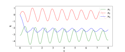
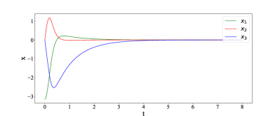
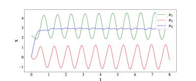
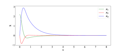
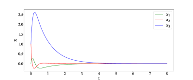
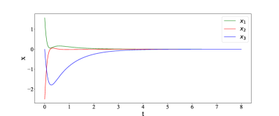
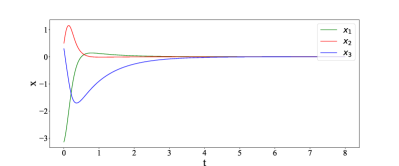
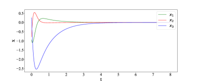
Using the trained NN approximation, we perform numerical simulations of the stabilization of the Reaction Wheel Pendulum. Recall that the approximate optimal feedback control law is given by (3.2), and the closed-loop stabilizing trajectories starting from $x_{0}$ can be numerically computed using the initial problem (3.4). Figure 3 shows the closed-loop trajectories from the NN feedback controllers at some points.

(a) $x_{0}=(0,1,1)$

(b) $x_{0}=(0.5\pi,-2.5,0)$

(c) $x_{0}=(-\pi,0.5,0.3)$

(d) $x_{0}=(-0.3\pi,-0.78,0.26)$

Figure 3. Sample closed-loop stabilizing trajectories of the Reaction Wheel Pendulum with different initial positions $x_{0}$ after the second round of training.

Remark 5.1.

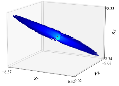
To explain the domain of attraction for the controller (3.2), we assume that $\mathcal{F}_{t}$ is the flow map given by (3.3). That is, for $x_{0}\in\mathbb{R}^{3}$, $t\in\mathbb{R}$, $\mathcal{F}_{t}(x_{0})=x(t,x_{0})$, where $x(t,x_{0})$ is the solution of (3.3) with $x(0)=x_{0}$. The domain of attraction is given by $\mathcal{F}_{t_{-}}(B_{0.5}(0))\cap\Omega$ with $t_{-}=-0.2$, where $\mathcal{F}_{t_{-}}(B_{0.5}(0))=\{x\in\mathbb{R}^{3}\,|\,x=\mathcal{F}_{t}(x_{0})\mbox{ for some }x_{0}\in B_{0.5}(0),t\in[-0.2,0]\}$ and $\Omega=[-3.2,3.2]\times[-3.2,3.2]\times[-3.2,3.2]$. It is clear that $B_{0.5}(0)\subset\mathcal{F}_{t_{-}}(B_{0.5}(0))$. Figure 4 provides a rough representation of the region $\mathcal{F}_{t_{-}}(B_{0.5}(0))$. If a larger domain is required, then a longer extension time $t_{-}$ and a larger restriction domain $\Omega$ should be chosen.

Figure 4. The region $\mathcal{F}_{-0.2}(B_{0.5}(0))$ in $\mathbb{R}^{3}$.

Furthermore, we compare the cost of the stable manifold (SM) method with the classical LQR and the optimal control obtained from the BVP solver. Table 1 shows the costs at several points. It is evident that the cost of the stable manifold method is much smaller than that of LQR and is very close to the optimal control obtained from the BVP solver when $|x_{0}|$ is relatively large, whereas the difference between the three costs is small when $x_{0}$ is near the origin. Note that here we obtain the optimal control based on the trained NN. Specifically, instead of using constants as the initial guess for the BVP solver, we use $(x^{NN}(t),p^{NN}(t))$ generated by the NN as the initial guess to solve the BVP (2.30)-(2.37) successfully.

Table 1. Comparison of the costs at certain points

Points	SM method	LQR	Optimal control
$(\pi,0,0)$	12.4	38.0	11.7
$(-0.8\pi,0.1,0.2)$	14.2	25.0	14.0
$(-0.6\pi,-0.2,-0.4)$	20.5	25.5	20.4
$(0.1\pi,0,0)$	0.8096	0.8115	0.8096
$(0.2,0.03,-0.08)$	0.4055	0.4060	0.4055

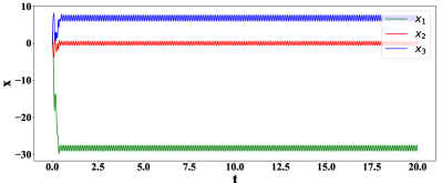
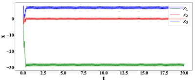
Finally, we illustrate the influence of rescaling. If we do not modify the model by rescaling at the beginning of the algorithm and keep all the parameters unchanged, then the NN approximation obtained cannot generate good feedback controllers. See Figure 5.

(a) $x_{0}=(\pi,0,0)$

(b) $x_{0}=(0.7\pi,0,0)$

Figure 5. Sample closed-loop trajectories after the second round of training without rescaling at the beginning.

6. Application to optimal control for the parabolic Allen-Cahn equation

In this section, to illustrate the effectiveness of our algorithm in high-dimensional optimal control problem, we give an application to optimal control of the parabolic Allen-Cahn equation as follows,

$$\partial_{t}\mathcal{X}(\gamma,t)=\sigma\partial_{\gamma\gamma}\mathcal{X}(\gamma,t)+\mathcal{X}(\gamma,t)-\mathcal{X}(\gamma,t)^{3}+u,$$

$$~{}~{}~{}~{}~{}~{}~{}~{}~{}~{}~{}~{}~{}~{}~{}~{}~{}~{}~{}~{}~{}~{}~{}~{}~{}~{}~{}~{}~{}~{}~{}~{}~{}~{}~{}~{}~{}~{}~{}~{}\mbox{ in }\mathcal{I}\times\mathbb{R}^{+},$$ (6.1)

$$\mathcal{X}(\gamma_{l},t)=0,\quad\mathcal{X}(\gamma_{r},t)=0,\quad t\in\mathbb{R}^{+},$$ (6.2)

$$\mathcal{X}(\gamma,0)=\mathcal{X}_{0},\quad\gamma\in\mathcal{I}.$$ (6.3)

Here $\mathcal{I}=[-1,1]$. The cost function is given by

$$J(u,\mathcal{X}_{0}):=\frac{1}{2}\int_{0}^{\infty}\left(\|\mathcal{X}(\cdot,t)\|^{2}_{L^{2}(\mathcal{I})}+\|u(t)\|_{L^{2}(\mathcal{I})}^{2}\right)dt.$$ (6.4)

The Allen-Cahn equation is a prototype equation that models a phase separation process ([16]). The optimal control of Allen-Cahn equations is a typical infinite dimensional control problem ([14, 13]). In this example, we approximate the Allen-Cahn equation by a high-dimensional system.

6.1. Difference approximation

Let $N$ be a positive integer greater than $3$, $h=\frac{2}{N}$ and

$$\gamma_{i}=-1+\frac{2i}{N},\quad i=0,1,\cdots,N.$$ (6.5)

Then

$$\mathcal{X}(\gamma_{0},t)=0,\quad\mathcal{X}(\gamma_{N},t)=0,$$ (6.6)

and for $i=1,\cdots,N-1$,

$$\mathcal{X}_{\gamma\gamma}(\gamma_{i})\approx\frac{1}{h^{2}}(\mathcal{X}(\gamma_{i+1})-2\mathcal{X}(\gamma_{i})+\mathcal{X}(\gamma_{i-1})).$$ (6.7)

Let

$$X(t)=(X_{1}(t),\cdots,X_{N-1}(t))=(\mathcal{X}(\gamma_{1},t),\cdots,\mathcal{X}(\gamma_{N-1},t)).$$

Hence from (6.5), (6.6), and (6.1)-(6.3), (6.7), we get

$$\mathcal{X}_{\gamma\gamma}\approx AX:=$$ (6.8)

$$\frac{1}{h^{2}}\left(\begin{array}[]{ccccccc}-2&1&0&0&\cdots&0&0\\ 1&-2&1&0&\cdots&0&0\\ 0&1&-2&1&\cdots&0&0\\ \vdots&\vdots&\vdots&\vdots&\vdots&\vdots&\vdots\\ 0&0&0&0&\cdots&1&-2\\ \end{array}\right)\left(\begin{array}[]{c}X_{1}\\ X_{2}\\ X_{3}\\ \vdots\\ X_{N-1}\\ \end{array}\right)$$ (6.19)

Set $u=(u_{1},u_{2},\cdots,u_{N-1})^{T}$. Then the control problem (6.1)-(6.3) becomes a discrete control system

$$\frac{d}{dt}X=\sigma AX+X-X^{3}+u,\quad X(0)=X_{0},$$

where the terms $X^{3}=(X_{1}^{3},\cdots,X_{N-1}^{3})$, and $X_{0}=(\mathcal{X}_{0}(\gamma_{1}),\,\cdots,\,\mathcal{X}_{0}(\gamma_{N-1}))$. Set

$$f(X)=(\sigma A+I_{N-1})X-X^{3}.$$

The corresponding cost function of (6.4) is

$$\frac{1}{2}\int_{0}^{\infty}\left(\sum_{i=1}^{N-1}X_{i}^{2}(t)h+\sum_{i=1}^{N-1}u_{i}^{2}h\right)dt$$

$$= \int_{0}^{\infty}\left(\frac{1}{N}\|X(t)\|^{2}+\frac{1}{N}\|u(t)\|^{2}\right)dt,$$

where $\|\cdot\|$ denotes the standard Euclid norm in $\mathbb{R}^{N-1}$.

6.2. The HJB equation

The corresponding HJB equation of the optimal control problem is

$$H(X,\nabla V)=$$ (6.20)

$$\nabla V^{T}(X)f(X)-\frac{1}{2}\nabla V^{T}(X)R\nabla V(X)+\frac{1}{N}X^{T}X=0.$$

Here

$$R:=\frac{N}{2}I_{N-1},$$ (6.21)

where $I_{N-1}$ is identity matrix of order $N-1$. The feedback controller is given by

$$u(x)=-\frac{N}{2}\nabla V(X).$$

The characteristic Hamiltonian system is

$$\left\{\begin{array}[]{l}\dot{X}=f(X)-RP\\ \dot{P}=-\dfrac{2}{N}X-\left(\dfrac{\partial f(X)}{\partial X}\right)^{T}P.\end{array}\right.$$ (6.24)

The Hamiltonian matrix is

$${\rm Ham}:=\left(\begin{array}[]{cc}\sigma A+I_{N-1}&-R\\ -\dfrac{2}{N}I_{N-1}&-\sigma A^{T}-I_{N-1}\\ \end{array}\right),$$ (6.27)

which is hyperbolic for any positive integer $N$ greater than 3.

6.3. Implementation of the algorithm

In the numerical experiment, we choose $N=31$ as an example. We utilize PyTorch to implement an NN, denoted as $p^{NN}(\theta,\cdot)$, with $L=2$ and $M=60$. The input data of the NN is a $30$-dimensional vector $x$, and its output is the approximation $p$ ($30$-dimensional). To be specific, we implement the NN function in the form of (4.2). Based on direct numerical computation, the Hamiltonian matrix is verified to be hyperbolic, with a gap of approximately $1.021$ between its spectrum and the imaginary axis. We employ the loss function of the form (4.3) with $\nu=1$, and set $\sigma_{1}=1$ and $\sigma_{2}=\sigma_{3}=0.1$. The NN approximation is trained using the algorithm presented in Section 4. Notably, we carry out the implementation of the algorithm on an ordinary laptop (ThinkPad T480s) without GPU acceleration.

6.4. Sampling, training and validation

To solve (2.30)-(2.37), we utilize the scipy.integrate.solve_bvp function with an error tolerance of $10^{-7}$. Since the distance between the eigenvalues and the imaginary axis is greater than $1.021$, we replace the infinite interval $[0,+\infty)$ with $[0,30]$ to ensure numerical accuracy. We use an initial mesh of $t$ given by $0,h,2h,\cdots,100h,$ where $h=0.3$, and the initial guess of the solution is set to $0$ at all nodes.

By performing a Monte Carlo test, we select a ball $B_{0.8}(0)\subset\mathbb{R}^{3}$, and randomly choose $1500$ points $x_{i}$ on the sphere $\partial B_{0.8}$ according to a uniform distribution. Here we utilize the norm in $\mathbb{R}^{30}$ defined as

$$|X|=\sqrt{\frac{1}{30}\sum_{i=1}^{30}X_{i}^{2}}.$$

We then use these points as initial conditions $x_{0}$ in (2.30)-(2.37). The BVP solver with these settings successfully solves the problem for all $1500$ initial conditions.

Next, we solve the initial value problem (4.7) using the scipy.integrate.solve_ivp function with the following settings: ‘method=Radau, rtol=$10^{-5}$ (relative tolerance), atol=$10^{-7}$ (absolute tolerance)’. From a Monte Carlo test, we have $T_{-}=-0.03$, and the IVP solver with these settings successfully solves the problem. As a result, we obtain $1500$ trajectories on the stable manifold.

Finally, we choose a sequence of $t$ given by $0=t_{1}<t_{2}<\cdots<t_{23}<30,$ where $t_{i}$ ($i=2,3,\cdots,23$) follows the exponential distribution (4.13) with $\lambda=1$. Furthermore, we select $3$ points uniformly at random from the negative interval $[-0.03,0]$. This results in a total of $39000$ samples on the stable manifold, denoted by the set $\mathcal{D}_{1}^{\rm train}$.

Following the same sampling procedure as described above, we solve $200$ trajectories on the stable manifold and select $26$ points on each trajectory. This results in a validation dataset $\mathcal{D}^{\rm val}$ with a total of $5200$ samples.

We use the internal optimizer Adam in PyTorch with a learning rate of $lr=0.01\times 0.5^{j}$ and train the NN for $6000$ epochs. Here, $j=[m/1500]$, where $m$ is the iterative times. After training, we achieve a small loss, with the train loss (4.3) on $\mathcal{D}_{1}^{\rm train}$ being $1.3\times 10^{-3}$ and the test loss on $\mathcal{D}^{\rm val}$ being $1.6\times 10^{-3}$. The training process takes approximately $5383$ seconds on a ThinkPad T480s laptop.

In this example, the first round training as described above resulted in a good approximation, with both the training loss and test loss being under $2\times 10^{-3}$. The subsequent simulations in the following subsection demonstrate the effectiveness of this approximate NN.

6.5. Simulations

In this subsection, we give simulations with various initial functions $\mathcal{X}_{0}$ to demonstrate the effectiveness of the feedback control generated from the trained NN.

In Figure 6 and Figure 7, we present a comparison between the dynamics of the uncontrolled system and the NN-controlled system. The simulations demonstrate that the NN-generated controller is effective in stabilizing the system.

Remark 6.1.

We mention that each evaluation of our NN-generated control signal takes on average less than one millisecond ($0.95\times 10^{-3}$ second) on a ThinkPad T480s laptop. This is significantly faster than the controllers presented in [37] and [33], whose time to generate control signals is at least several milliseconds. This fast control signal generation time is crucial for real-time applications.

(a) Uncontrolled dynamics

(b) Controlled dynamics

Figure 6. The dynamics of the uncontrolled system and NN controlled system with initial state $\mathcal{X}_{0}=3.5\cos(1.5\pi x)$.

(a) Uncontrolled dynamics

(b) Controlled dynamics

Figure 7. The dynamics of the uncontrolled system and NN controlled system with initial state $\mathcal{X}_{0}=2(x^{2}-1)$.

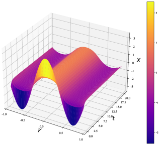
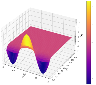
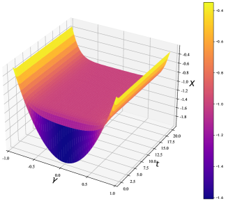
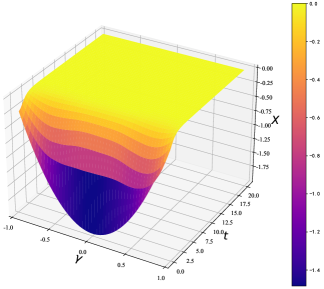
Finally, we compare the cost of the NN-generated controller, the LQR, and the standard BVP solver. When the initial function is large, the cost of the NN-generated feedback controller is much smaller than that of the LQR, and is very close to that of the standard BVP solver. When the initial point is close to the equilibrium, the costs of these three cases are almost the same. This is an obvious fact from a theoretical point of view. It is worth noting that, as in the example of the control of the wheel reaction pendulum, we use $(x^{NN}(t),p^{NN}(t))$ generated by the trained NN as the initial guess to solve the BVP (2.30)-(2.37).

Table 2. Comparison of the costs for certain initial states

Points	SM method	LQR	Optimal control
$3.5\cos(1.5\pi x)$	1.91	3.36	1.86
$2(x^{2}-1)$	2.04	2.92	1.96
$2.5(x-1)(x+1)^{3}$	2.15	4.39	2.10
$0.3\sin(\pi x)$	0.09673	0.09678	0.09667
$0.5(x-1)(x+1)^{3}$	0.0488	0.0513	0.0488

7. Conclusion

In this paper, we provide a theoretical proof that, under some natural conditions, neural network approximations of the stable manifold of the HJB equation can generate nearly optimal controllers. Our theoretical analysis verifies that the approximate NN-controlled system is exponentially stable at the origin as $t$ tends to $+\infty$.

Based on this theoretical conclusion, we propose an algorithm to construct a type of deep NN semiglobal approximations for the stable manifold. Our method relies on the geometric properties of the HJB equations, and the main advantage is that the derivatives of the value function of the optimal problem need not be calculated in the training procedure and computation of feedback control. We use adaptive data generation by finding trajectories in the stable manifold based on a combination of two-point boundary value problems (BVP) near the equilibrium and initial value problems (IVP) far away from the equilibrium for the Hamiltonian systems of the HJB equations. We randomly select a certain number of samples on each trajectory, which allows the data set to inherit the geometric features of the stable manifold and reduce the computation cost of data generation. The adaptive samples are chosen near the points with large errors after the previous round of training to rapidly improve the accuracy of the NN approximations.

We illustrate the effectiveness of our framework by stabilizing the Reaction Wheel Pendulum and seeking optimal control of the parabolic Allen-Cahn equation. The simulations demonstrate that our approach has good performance. The algorithm is causality-free and adaptive sampling, and it is suitable for high-dimensional systems.

It is worth noting that similar analysis and algorithms may be used for systems with other geometric features, such as Lie group symmetry or contact geometry. These topics deserve further exploration.

Appendix A Proof of Theorem 3.2 and Corollary 3.2

Proof of Theorem 3.2.

Inspired by [11, Proof of Theorem 2.77], we give a proof which focuses on the perturbation feature of the equations.

Recalling that $f(x)=Ax+O(|x|^{2})$, $R(x)=R(0)+O(|x|)$, $p(x)=Px+O(|x|^{2})$ and $B=A-R(0)P$, we rewrite (3.3) and (3.4) as

$$\dot{x} = Bx+(f(x)-Ax)-(R(x)p(x)-R(0)Px)$$ (A.1)

$$:= Bx+n(x),\,x(0)=x_{0}$$

and

$$\dot{x} = Bx+(f(x)-Ax)-(R(x)p^{NN}(\theta,x)-R(0)Px)$$ (A.2)

$$:= Bx+n^{NN}(x),\,x(0)=x_{0}.$$

1. Note that

$$x(t)=e^{Bt}x_{0}+\int_{0}^{t}e^{B(t-s)}n(x(s))ds$$

and

$$x^{NN}(t)=e^{Bt}x_{0}+\int_{0}^{t}e^{B(t-s)}n^{NN}(x^{NN}(s))ds.$$

It follows that

$$x^{NN}(t)-x(t)\\ =\int_{0}^{t}e^{B(t-s)}(n^{NN}(x^{NN}(s))-n(x(s)))ds.$$

We first assume $x^{NN}(t)\in\Omega$. Hence

$$|R(x^{NN}(t))|<C,\quad|p(x^{NN}(t))|<C,$$

$$|R(x^{NN}(t))-R(x(t))|\leq L|x^{NN}(t)-x(t)|.$$

From the Condition (a) in Theorem 3.2, we have

$$\left|n^{NN}(x^{NN}(s))-n(x(s))\right|$$

$$\leq |f(x^{NN})-f(x)|+|R(x^{NN})|\cdot$$

$$\quad\quad\quad|p^{NN}(\theta,x^{NN})-p(x^{NN})|$$

$$+|p(x^{NN})||R(x^{NN})-R(x)|$$

$$+|R(x)||p(x^{NN})-p(x)|\leq CL|x^{NN}-x|+C\delta.$$

Using (3.7), it holds that

$$|x^{NN}(t)-x(t)|$$

$$\leq \int_{0}^{t}e^{-\beta(t-s)}(CL|x^{NN}(s)-x(s)|+C\delta)ds$$

$$\leq C\beta^{-1}\delta+C\int_{0}^{t}Le^{-\beta(t-s)}|x^{NN}(s)-x(s)|ds.$$

Set $y(t)=|x^{NN}(t)-x(t)|$. Hence

$$y(t)\leq C\beta^{-1}\delta+\int_{0}^{t}CLe^{-\beta(t-s)}y(s)ds.$$ (A.3)

Some direct computations yield that

$$\frac{d}{dt}\left(C\beta^{-1}\delta+\int_{0}^{t}CLe^{-\beta(t-s)}y(s)ds\right)$$

$$= CLy(t)-\beta\int_{0}^{t}CLe^{-\beta(t-s)}y(s)ds$$

$$\leq CLy(t)\leq CL(C\beta^{-1}\delta+\int_{0}^{t}CLe^{-\beta(t-s)}y(s)ds).$$

Hence

$$\frac{d}{dt}\log\left(C\beta^{-1}\delta+\int_{0}^{t}CLe^{-\beta(t-s)}y(s)ds\right)\leq CL.$$

We obtain

$$\log\left(C\beta^{-1}\delta+\int_{0}^{t}CLe^{-\beta(t-s)}y(s)ds\right)$$

$$\leq \log(C\beta^{-1}\delta)+CLt.$$

By (A.3),

$$|x^{NN}(t)-x(t)|=y(t)\leq C\beta^{-1}\delta e^{CLt}.$$ (A.4)

Using (3.8), it holds that for $\delta<C^{-1}\beta e^{-CLT_{\varepsilon}}\varepsilon/2$,

$$|x^{NN}(t)-x(t)|<\varepsilon/2,$$ (A.5)

$$|x^{NN}(T_{\varepsilon})|<\varepsilon,\mbox{ and, }x^{NN}(t)\in\Omega,\mbox{ for all }t\in[0,T_{\varepsilon}],$$

provided some $0<\varepsilon<\gamma_{0}$. Hence the assumption at the beginning of the proof is satisfied if $x(0)=x_{0}\in\Omega:=\{x\in\Omega\,|\,{\rm dist}(x,\partial\Omega)<\varepsilon\}$. Here ${\rm dist}(x,\partial\Omega)<\varepsilon\}$ denotes the distance between $x$ and the boundary of $\Omega$.

2. Let $\varepsilon_{0}$ be an some positive constant sufficiently small in $(0,\gamma_{0})$, and let $\varepsilon<\varepsilon_{0}$. Assume $I=\{t\geq T_{\varepsilon}\,|\,|x^{NN}(t)|<\varepsilon_{0}\}$. Moreover, we have

$$x^{NN}(t)=e^{Bt}x^{NN}(T_{\varepsilon})+\int_{T_{\varepsilon}}^{t}e^{B(t-s)}n^{NN}(x^{NN}(s))ds.$$

For $t\in I$, since $|p^{NN}(\theta,x^{NN}(t))-Px^{NN}(t)|\leq\eta|x^{NN}(t)|$ (Condition (b) in Theorem 3.2), it holds that

$$|n^{NN}(x^{NN}(t))|$$

$$\leq |f(x^{NN}(t))-Ax^{NN}(t)|$$

$$+|(R(x^{NN}(t))p^{NN}(\theta,x^{NN}(t))-R(0)Px^{NN}(t)|$$

$$\leq k|x^{NN}(t)|^{2}+|R(x^{NN}(t))-R(0)||Px^{NN}(t)|$$

$$+|R(x^{NN}(t))||p^{NN}(\theta,x^{NN}(t))-Px^{NN}(t)|$$

$$\leq C_{1}((k+1)\varepsilon_{0}+\eta)|x^{NN}(t)|,$$

where $C_{1}$ is a constant depending only on $f,R,p$. It follows that

$$|x^{NN}(t)| \leq C|x^{NN}(T_{\varepsilon})|e^{-\beta(t-T_{\varepsilon})}$$

$$+C\int_{T_{\varepsilon}}^{t}e^{-\beta(t-s)}|n^{NN}(x^{NN}(s))|ds$$

$$\leq C|x^{NN}(T_{\varepsilon})|e^{-\beta(t-T_{\varepsilon})}$$

$$+CC_{1}((k+1)\varepsilon_{0}+\eta)\int_{T_{\varepsilon}}^{t}e^{-\beta(t-s)}|x^{NN}(s)|ds.$$

Using the Gronwall inequality, we find that

$$|x^{NN}(t)| \leq C|x^{NN}(T_{\varepsilon})|e^{-(\beta-CC_{1}((k+1)\varepsilon_{0}+\eta))(t-T_{\varepsilon})}$$ (A.6)

$$= C|x^{NN}(T_{\varepsilon})|e^{-\alpha(t-T_{\varepsilon})},$$

where $\alpha=\beta-CC_{1}((k+1)\varepsilon_{0}+\eta)$. If we choose the two positive constants $\varepsilon_{0},\eta$ sufficiently small, then $\alpha>0$. In the following, we assume that the consant $C$ in (A.6) is greater than 2.

3. We prove that for $\varepsilon<\varepsilon_{0}/C$, $I=[T_{\varepsilon},\infty)$. If not, then there exists a $\bar{T}<\infty$ such that $J=[T_{\varepsilon},\bar{T})$. Since $|x^{NN}(T_{\varepsilon})|<\varepsilon_{0}/C$, from (A.6) we get that

$$|x^{NN}(t)|<\varepsilon_{0}e^{-\alpha(t-T_{\varepsilon})}<\varepsilon_{0},\quad\forall t\in[T_{\varepsilon},\bar{T}).$$

Then by the extension theorem of ODE, there is some small $\tau>0$ such that the solution is defined in the $[T_{\varepsilon},\bar{T}+\tau)$ and

$$|x^{NN}(t)|\leq\varepsilon_{0}e^{-\alpha(t-T_{\varepsilon})}<\varepsilon_{0},\quad\forall t\in[T_{\varepsilon},\bar{T}+\tau).$$

That is a contradiction by the definition of $I$.

4. In summary, let $C$ be fixed constant in (A.6) larger than $2$, and let $\varepsilon_{0}$ be a constant in $(0,\gamma_{0})$ sufficiently small. For $0<\varepsilon<\varepsilon_{0}/C<\gamma_{0}$ and $\delta<C^{-1}\beta e^{-CLT_{\varepsilon}}\varepsilon/2$, we have that

$$|x^{NN}(t)-x(t)|\leq\varepsilon_{0},\quad\forall t\in(0,\infty),$$

and

$$|x^{NN}(t)|<\varepsilon_{0}e^{-\alpha(t-T_{\varepsilon})},\quad\forall t\in(T_{\varepsilon},\infty).$$

That yields the result in Theorem 3.2. ∎

Proof of Corollary 3.2.

From the proof of Theorem 3.2, we have that

$$|q(x^{NN})-q(x)|\leq 2|Q||x||x^{NN}-x|\leq C|x^{NN}-x|,$$

and

$$|u^{NN}(x^{NN})-u(x)|$$

$$\leq |W^{-1}|[(|g(x^{NN})-g(x)||p^{NN}(x^{NN})|+$$

$$|g(x)||p^{NN}(x^{NN})-p(x^{NN})|+|g(x)||p(x^{NN})-p(x)|)]$$

$$\leq C(|x^{NN}-x|+\delta),$$

where $C>0$ is a constant depending only on $g,p,W$. Hence by Theorem 3.2, for $\delta>0$ sufficiently small, it holds that for some $\varepsilon_{0}<\gamma_{0}$,

$$|J(x^{NN},u^{NN})-J(x,u)|\leq C_{2}\varepsilon_{0},$$ (A.7)

where $C_{2}$ is a constant depending only on $f,g,R,p,W$. This completes the proof. ∎

References

- [1] David Angeli. Almost global stabilization of the inverted pendulum via continuous state feedback. Automatica, 37(7):1103–1108, 2001.
- [2] Karl Johan Åström, J Aracil, F Gordillo, et al. A family of smooth controllers for swinging up a pendulum. Automatica, 44(7):1841–1848, 2008.
- [3] Karl Johan Åström and Katsuhisa Furuta. Swinging up a pendulum by energy control. Automatica, 36(2):287–295, 2000.
- [4] Randal W. Beard, George N. Saridis, and John T. Wen. Galerkin approximations of the generalized Hamilton-Jacobi-Bellman equation. Automatica, 33(12):2159–2177, 1997.
- [5] Daniel J Block, Karl J Åström, and Mark W Spong. The reaction wheel pendulum. Synthesis Lectures on Control and mechatronics, 1(1):1–105, 2007.
- [6] Olivier Bokanowski, Jochen Garcke, Michael Griebel, and Irene Klompmaker. An adaptive sparse grid semi-lagrangian scheme for first order Hamilton-Jacobi-Bellman equations. Journal of Scientific Computing, 55(3):575–605, 2013.
- [7] Simone Cacace, Emiliano Cristiani, Maurizio Falcone, and Athena Picarelli. A patchy dynamic programming scheme for a class of Hamilton–Jacobi–Bellman equations. SIAM Journal on Scientific Computing, 34(5):A2625–A2649, 2012.
- [8] Piermarco Cannarsa and Wei Cheng. Singularities of Solutions of Hamilton–Jacobi Equations. Milan Journal of Mathematics, 89(1):187–215, 2021.
- [9] Nalin A Chaturvedi, N Harris McClamroch, Dennis S Bernstein. Asymptotic smooth stabilization of the inverted 3-D pendulum. IEEE Transactions on Automatic Control, 54(6):1204–1215, 2009.
- [10] Guoyuan Chen and Gaosheng Zhu. Symplectic algorithms for stable manifolds in control theory. IEEE Transactions on Automatic Control, 67(6), 3105–3111, 2022.
- [11] Carmen Chicone. Ordinary differential equations with applications, volume 34. Springer Science & Business Media, 2006.
- [12] Yat Tin Chow, Jérôme Darbon, Stanley Osher, and Wotao Yin. Algorithm for overcoming the curse of dimensionality for state-dependent Hamilton-Jacobi equations. Journal of Computational Physics, 387:376–409, 2019.
- [13] Konstantinos Chrysafinos and Dimitra Plaka. Analysis and approximations of an optimal control problem for the Allen-Cahn equation. arXiv preprint arXiv:2202.09149, 2022.
- [14] Pierluigi Colli and Jurgen Sprekels. Optimal control of an Allen–Cahn equation with singular potentials and dynamic boundary condition. SIAM Journal on Control and Optimization, 53(1):213–234, 2015.
- [15] Jérôme Darbon and Stanley Osher. Algorithms for overcoming the curse of dimensionality for certain Hamilton–Jacobi equations arising in control theory and elsewhere. Research in the Mathematical Sciences, 3(1):19, 2016.
- [16] Qiang Du and Xiaobing Feng. The phase field method for geometric moving interfaces and their numerical approximations. Handbook of numerical analysis, 21: 425–508, 2020.
- [17] Weinan E, Jiequn Han, Arnulf Jentzen. Algorithms for solving high dimensional PDEs: from nonlinear Monte Carlo to machine learning. Nonlinearity, 35(1):278, 2021.
- [18] Jiequn Han, Arnulf Jentzen, and Weinan E. Solving high-dimensional partial differential equations using deep learning. Proceedings of the National Academy of Sciences, 115(34):8505–8510, 2018.
- [19] Sepp Hochreiter and Jürgen Schmidhuber. Long short-term memory. Neural computation, 9(8):1735–1780, 1997.
- [20] T. Horibe and N. Sakamoto. Nonlinear optimal control for swing up and stabilization of the acrobot via stable manifold approach: Theory and experiment. IEEE Transactions on Control Systems Technology, 27(6):2374–2387, Nov 2019.
- [21] Takamasa Horibe and Noboru Sakamoto. Optimal swing up and stabilization control for inverted pendulum via stable manifold method. IEEE Transactions on Control Systems Technology, 26(2):708–715, 2017.
- [22] Kurt Hornik. Approximation capabilities of multilayer feedforward networks Neural networks, 4(2):251–257, 1991.
- [23] Dario Izzo, Ekin Öztürk, and Marcus Märtens. Interplanetary transfers via deep representations of the optimal policy and/or of the value function. In Proceedings of the Genetic and Evolutionary Computation Conference Companion, pages 1971–1979, 2019.
- [24] Frank Jiang, Glen Chou, Mo Chen, and Claire J Tomlin. Using neural networks to compute approximate and guaranteed feasible Hamilton-Jacobi-Bellman PDE solutions. arXiv preprint arXiv:1611.03158, 2016.
- [25] Eric Jones, Travis Oliphant, Pearu Peterson, et al. Scipy: Open source scientific tools for python. 2001.
- [26] Dante Kalise and Karl Kunisch. Polynomial approximation of high-dimensional Hamilton–Jacobi–Bellman equations and applications to feedback control of semilinear parabolic pdes. SIAM Journal on Scientific Computing, 40(2):A629–A652, 2018.
- [27] Wei Kang, Qi Gong, and Tenavi Nakamura-Zimmerer. Algorithms of data development for deep learning and feedback design. arXiv preprint arXiv:1912.00492, 2019.
- [28] Wei Kang and Lucas Wilcox. A causality free computational method for HJB equations with application to rigid body satellites. In AIAA Guidance, Navigation, and Control Conference, page 2009, 2015.
- [29] Wei Kang and Lucas C Wilcox. Mitigating the curse of dimensionality: sparse grid characteristics method for optimal feedback control and HJB equations. Computational Optimization and Applications, 68(2):289–315, 2017.
- [30] Wei Kang and Lucas C Wilcox. Solving 1d conservation laws using Pontryagin Minimum Principle. Journal of Scientific Computing, 71(1):144–165, 2017.
- [31] Karl Kunisch and Daniel Walter. Semiglobal optimal feedback stabilization of autonomous systems via deep neural network approximation. ESAIM: Control, Optimisation and Calculus of Variations, Vol. 27, artical number 16, 2021.
- [32] William M. McEneaney. A curse-of-dimensionality-free numerical method for solution of certain HJB PDEs. SIAM Journal on Control and Optimization, 46(4):1239–1276, 2007.
- [33] Tenavi Nakamura-Zimmerer, Qi Gong, and Wei Kang. Adaptive deep learning for high dimensional Hamilton-Jacobi-Bellman equations. SIAM Journal on Scientific Computing, Vol. 43(2):A1221–A1247, 2021.
- [34] Tenavi Nakamura-Zimmerer, Qi Gong, and Wei Kang. Neural network optimal feedback control with guaranteed local stability. IEEE Open Journal of Control Systems, Vol. 1: 210–222, 2022.
- [35] Carmeliza Navasca and Arthur J Krener. Patchy solutions of Hamilton-Jacobi-Bellman partial differential equations. In Modeling, estimation and control, pages 251–270. Springer, 2007.
- [36] Toshiyuki Ohtsuka. Solutions to the Hamilton-Jacobi equation with algebraic gradients. IEEE Transactions on Automatic Control, 56(8):1874–1885, 2010.
- [37] Derek Onken, Levon Nurbekyan, Xingjian Li, Samy Wu Fung, Stanley Osher, and Lars Ruthotto. A neural network approach for high-dimensional optimal control applied to multiagent path finding. IEEE Transactions on Control Systems Technology, (To appear):1–17, 2022.
- [38] Tomaso Poggio, Hrushikesh Mhaskar, Lorenzo Rosasco, Brando Miranda and Qianli Liao. Why and when can deep-but not shallow-networks avoid the curse of dimensionality: a review. International Journal of Automation and Computing, 14(5):503–519, 2017.
- [39] Maziar Raissi. Forward-backward stochastic neural networks: Deep learning of high-dimensional partial differential equations. arXiv preprint arXiv:1804.07010, 2018.
- [40] I Michael Ross, Qi Gong, and Pooya Sekhavat. Low-thrust, high-accuracy trajectory optimization. Journal of Guidance, Control, and Dynamics, 30(4):921–933, 2007.
- [41] IM Ross, Q Gong, M Karpenko, and RJ Proulx. Scaling and balancing for high-performance computation of optimal controls. Journal of Guidance, Control, and Dynamics, 41(10):2086–2097, 2018.
- [42] Noboru Sakamoto. Case studies on the application of the stable manifold approach for nonlinear optimal control design. Automatica, 49(2):568–576, 2013.
- [43] Noboru Sakamoto and Arjan J van der Schaft. Analytical approximation methods for the stabilizing solution of the Hamilton–Jacobi equation. IEEE Transactions on Automatic Control, 53(10):2335–2350, 2008.
- [44] L Shampine and J Kierzenka. A BVP solver based on residual control and the MATLAB PSE. ACM Trans. Math. Software, 27:299–315, 2001.
- [45] Justin Sirignano and Konstantinos Spiliopoulos. DGM: A deep learning algorithm for solving partial differential equations. Journal of Computational Physics, 375:1339–1364, 2018.
- [46] Mark W Spong, Peter Corke, and Rogelio Lozano. Nonlinear control of the reaction wheel pendulum. Automatica, 37(11):1845–1851, 2001.
- [47] Yuval Tassa and Tom Erez. Least squares solutions of the HJB equation with neural network value-function approximators. IEEE transactions on neural networks, 18(4):1031–1041, 2007.
- [48] Arjan J. van der Schaft. On a state space approach to nonlinear control. Systems & Control Letters, 16(1):1–8, 1991.
- [49] Ivan Yegorov and Peter M Dower. Perspectives on characteristics based curse-of-dimensionality-free numerical approaches for solving Hamilton–Jacobi equations. Applied Mathematics & Optimization, pages 1–49, 2018.