Morphological and non-equilibrium analysis of coupled Rayleigh-Taylor-Kelvin-Helmholtz instability

Abstract

In this paper, the coupled Rayleigh-Taylor-Kelvin-Helmholtz instability(RTI, KHI and RTKHI, respectively) system is investigated using a multiple-relaxation-time discrete Boltzmann model. Both the morphological boundary length and thermodynamic non-equilibrium (TNE) strength are introduced to probe the complex configurations and kinetic processes. In the simulations, RTI always plays a major role in the later stage, while the main mechanism in the early stage depends on the comparison of buoyancy and shear strength. It is found that, both the total boundary length $L$ of the condensed temperature field and the mean heat flux strength $D_{3,1}$ can be used to measure the ratio of buoyancy to shear strength, and to quantitatively judge the main mechanism in the early stage of the RTKHI system. Specifically, when KHI (RTI) dominates, $L^{KHI}>L^{RTI}$ ($L^{KHI}<L^{RTI}$), $D_{3,1}^{KHI}>D_{3,1}^{RTI}$ ($D_{3,1}^{KHI}<D_{3,1}^{RTI}$); when KHI and RTI are balanced, $L^{KHI}=L^{RTI}$, $D_{3,1}^{KHI}=D_{3,1}^{RTI}$, where the superscript, “KHI (RTI) " , indicates the type of hydrodynamic instability. It is interesting to find that, (i) for the critical cases where KHI and RTI are balanced, both the critical shear velocity $u_{C}$ and Reynolds number $Re$ show a linear relationship with the gravity/accelaration $g$; (ii) the two quantities, $L$ and $D_{3,1}$, always show a high correlation, especially in the early stage where it is roughly $0.999$, which means that $L$ and $D_{3,1}$ follows approximately a linear relationship. The heat conduction has a significant influence on the linear relationship. A second sets of findings are as below: For the case where the KHI dominates at earlier time and the RTI dominates at later time, the evolution process can be roughly divided into two stages. Before the transition point of the two stages, $L^{RTKHI}$ initially increases exponentially, and then increases linearly. Hence, the ending point of linear increasing $L^{RTKHI}$ can work as a geometric criterion for discriminating the two stages. The TNE quantity, heat flux strength $D_{3,1}^{RTKHI}$, shows similar behavior. Therefore, the ending point of linear increasing $D_{3,1}^{RTKHI}$ can work as a physical criterion for discriminating the two stages.

I Introduction

Hydrodynamic instabilities are prevalent in various natural and technological environments. The Rayleigh-Taylor instability (RTI) occurs at a perturbed interface when a heavy fluid is accelerated or supported by a light one in a force field. The Kelvin-Helmholtz instability (KHI) occurs when there is a tangential velocity difference between two fluids separated by a perturbed interface. In the nonlinear evolution of RTI, the KHI will develop as a secondary instability at the high-density spike tips where the velocity shear is strong, and forms the resulted classical mushroom structures. Similarly, in the nonlinear evolution of KHI, the secondary RTI starts to develop along the vortex arms, due to the centrifugal acceleration of the rotating KHI vortex, when the density variation of the two fluids is large enough Faganello, Califano, and Pegoraro (2008). In addition, for a more general case, the coupled RTI and KHI are prevalent in various real systems, such as in the atmosphere and oceans, air/fuel mixing in combustion chambers, the outer region of supernovae, and the compression of the fuel capsule in inertial confinement fusion. Thus, it is a practical and inevitable problem to understand the behaviors of coupled Rayleigh-Taylor-Kelvin-Helmholtz instability (RTKHI).

Extensive efforts have been devoted to experimental and computational studies of the phenomena. Lawrence et al. Lawrence, Browand, and Redekopp (1991) performed a stability analysis on the coupled instability by solving the Taylor-Goldstein equation, compared with experiments performed in mixing layer channels, and discovered the transformation from shear instability dominated flow to RTI dominated flow. A linear analysis of the hybrid KHI and RTI in an electrostatic magnetosphere-ionosphere coupling system was carried out by Yamamoto Yamamoto (2008). The combined RTI and KHI of two superimposed magnetized fluids in the presence of suspended dust particles had been investigated by Prajapati et alPrajapati et al. (2009). Guglielmi et al. discussed the coupled RTKHI at the magnetopauseGuglielmi, Potapov, and Klain (2010), and the possible geophysical applications to the theory (e.g., penetration of the solar plasma into the magnetosphere, excitation of global Pc5 oscillations) were indicated. Ye et al. Wang, Ye, and Li (2010); Ye et al. (2011) investigated analytically the competitions between RTI and KHI in two-dimensional incompressible fluids within a linear growth regime. It is found that the competition between the RTI and the KHI is dependent on the Froude number, the density ratio of the two fluids, and the thicknesses of the density transition layer and the velocity shear layer. Mandal et al. Mandal et al. (2011) investigated the nonlinear evolution of two fluid interfacial structures such as bubbles and spikes arising due to the combined action of RTI and KHI. Olson et al. Olson et al. (2011) studied the coupled RTKHI in the early nonlinear regime through Large eddy simulation. Numerical simulations showed a complex and non-monotonic behavior where small amounts of shear in fact decrease the growth rate, and the physical origins of this non-monotonic behavior were investigated. Dolai et al. Dolai, Prajapati, and Chhajlani (2016) investigated the effect of different dust flow velocities and two dimensional magnetic fields on the combined KHI and RTI of two superimposed incompressible dusty fluids. Vadivukkarasan et al. Vadivukkarasan and Panchagnula (2016, 2017) described the three-dimensional destabilization characteristics of cylindrical and annular interfaces under the combined action of RTI and KHI mechanisms, by introducing dimensionless numbers such as Bond number, inner and outer Weber numbers and inner and outer density ratio. Sarychev et al. Sarychev et al. (2019) found that an undulating topography on the interface coating/base material resulted from a combination of Rayleigh-Taylor and Kelvin-Helmholtz instabilities.

When studying the coupled instability, the Richardson number $Ri$ is often used to quantify this transition from KHI-like to RTI-like behavior, and has been discussed by many authors Snider and Andrews (1996); Akula, Andrews, and Ranjan (2013); Akula and Ranjan (2016); Akula et al. (2017); Finn (2014). Akula et al. identified a similar transition from KHI-like to RTI-like instability growth used a gas tunnel facility, determined a transitional Richardson number of $-1.5$ to $-2.5$ in an early research Akula, Andrews, and Ranjan (2013), and $-0.17$ to $-0.56$ in later experiments ($At$ from $0.035$ to $0.159$) Akula et al. (2017). Finn Finn (2014) performed an experimental study of the combined RTI and KHI at three different Atwood numbers ($0.05$, $0.971$, $0.147$), and found that the transition occurs between the values of $-0.25$ and $-1.0$.

Besides the Hydrodynamic Non-Equilibrium (HNE) behaviors, the most relevant Thermodynamic Non-Equilibrium (TNE) behaviors in various complex flow systems, including systems with hydrodynamic instabilities, are attracting more attention with time Xu, Zhang, and Ying (2015); Xu, Zhang, and Gan (2016); Xu, Zhang, and Zhang (2018). When the TNE is very weak, the loss of considering TNE does not make much difference. But when the TNE is strong, the situation will be greatly different. For example, the existence of TNE directly affects the density, temperature and pressure, as well as the magnitude and direction of flow velocity. Without considering TNE, the density, flow velocity, temperature and pressure given will have a significant deviation Lin and Luo (2019). The existence of TNE is the underlying cause of heat flux and viscous stress. If insufficiently considered (considered only the linear response part), the amplitude of heat flow and stress obtained may be too largeGan et al. (2018). When the strength of TNE beyond some threshold values, it may change the directions of heat flow and stress. If not sufficiently considered (considered only the linear response part), the resulting stress and heat flow, even in the wrong directions, may be obtained Zhang et al. (2019a). In addition, in phase separation system, both the mean TNE strength Gan et al. (2015) and the entropy production rate Zhang et al. (2019b) increase with time in the spinodal decomposition stage and decrease with time in the domain growth stage, therefore, both the peak value points of the mean TNE strength and the entropy production rate can work as physical criteria to discriminate the two stages Gan et al. (2015); Xu, Zhang, and Gan (2016); Zhang et al. (2019b). In system with combustion, the TNE behaviors help to better understand the physical structures of the von Neumann peak and various non-equilibrium detonation Xu, Zhang, and Ying (2015); Yan et al. (2013); Xu et al. (2015); Lin et al. (2016); Zhang et al. (2016); Lin and Luo (2018); Lin et al. (2017a); Xu et al. (2018a); Lin and Luo (2019). For droplet collision, TNE behavior can be used to identify the different stages of the collision process and to distinguish different types of collision Zhang et al. . In system with RTI, the TNE behaviors around interfaces have been used to physically identify and distinguish various interfaces and design relevant interface-tracking schemes. All the TNE kinetic modes become stronger as the compressibility increases. Some TNE kinetic modes remain always in small amplitudes. With increasing the compressibility, more observable TNE kinetic modes appear for given observation precisionLai et al. (2016); Xu, Zhang, and Zhang (2018). The correlation between the mean density nonuniformity and mean TNE strength is almost 1. The correlation between the mean temperature nonuniformity and mean Non-Organized Energy Flux (NOEF) is almost 1, and the correlation between the mean flow velocity nonuniformity and the mean Non-Organized Momentum Flux (NOMF) is also high, but generally less than 1 Chen, Xu, and Zhang (2016); Xu, Zhang, and Zhang (2018). The TNE effect helps to understand the effect of system dispersion (desctibed by $Kn$ number) on its kinetic behaviorsYe et al. (2020). In system with pure KHI, via some defined TNE quantity, for example, the heat flux intensity, we can observe simultaneously the density interface and temperature interface so that we can investigate simultaneously the material mixing and energy mixing in the KHI evolution Zhang et al. (2019a); Gan et al. (2019). The TNE behaviors were used to better understand the mixing entropy in multi-component flowsLin et al. (2017b). In this work, we will show that, the endpoint of the NOEF, one of the various TNE effects, intensity linear growth stage can be used as a physical criterion from KHI-dominated to RTI-dominated in RTKHI coexistence systems.

Since the traditional hydrodynamic model is incapable of capturing the TNE behaviors, the above TNE combined by HNE studies resorted to a coarse-grained model derived from the Boltzmann equation, the discrete Boltzmann model (DBM) Xu, Zhang, and Ying (2015); Xu, Zhang, and Gan (2016); Xu, Zhang, and Zhang (2018), developed from the well-known lattice Boltzmann method Succi (2001); Benzi, Succi, and Vergassola (1992); Xu et al. (2012); Osborn et al. (1995); Li et al. (2004); Zhang, Qin, and Emerson (2005); Shan, Yuan, and Chen (2006); Wang et al. (2015); Qu, Shu, and Chew (2007); Zhuo, Zhong, and Gao (2012); Li and Zhong (2015); Zhang et al. (2005); Xia et al. (2015); Chen, Xia, and Cai (2010); Ambruş and Sofonea (2019); Busuioc and Ambruş (2019); Ambruş, Sharipov, and Sofonea (2020); Gabbana et al. (2020); Wang, Wei, and Qian (2020); Chen, Shu, and Tan (2018); Wang et al. (2020); Chen, Shu, and Zhang (2019); Xu, Yu, and Regenauer-Lieb (2020); Saadat and Karlin (2020); Wang, Tan, and Phan-Thien (2019); Fei et al. (2019). DBM is inspired by refining measurement step-by-step modeling scenario which is indicated by Chapman-Enskog (CE) multi-scale expansion. There are infinitely many specific ways to progressively refine the measurement, and CE describes one of them. In the case of the validity of CE theory, DBM construction can quickly confirm the necessary kinetic relations to be preserved by virtue of it, but, in principle, CE is only one of the candidate references. DBM, being different from the macroscopic fluid equations derived from CE in some aspects, shows physical advantages via the differences. The DBM has emerged as a feasible computational tool for describing the kinetic behaviors of complex systems. Besides recovering the macroscopic hydrodynamic equations in the continuum limit, DBM presents more kinetic information on the non-equilibrium effects which are generally related to some mesoscopic structures and/or kinetic modes Xu, Zhang, and Ying (2015); Xu, Zhang, and Gan (2016); Xu, Zhang, and Zhang (2018). In 2012, Xu et al. Xu et al. (2012) pointed out that, according to the non-equilibrium statistical physics, the nonconserved kinetic moments of $(f-f^{eq})$ can be applied to describe more specifically how the system deviates from its thermodynamic equilibrium state and to extract more specific information on the effects resulted from this deviation, where $f$ is the distribution function and $f^{eq}$ is the corresponding local equilibrium distribution function. $f$ and $f^{eq}$ share the same conserved kinetic moments, including the density, momentum and energy. Then, it was suggested to investigate the complex TNE behaviors in the phase space opened by the independent components of the nonconserved kinetic moments of $(f-f^{eq})$ and its subspacesXu et al. (2015). In the phase space opened by nonconserved kinetic moments and its subspaces, corresponding non-equilibrium strength was defined by means of the distance from the origin, and non-equilibrium state similarity and kinetic process similarity were defined by means of the reciprocal of the distance between two points Xu et al. (2015, 2018b). Via those concepts some previously unextractable information can be hierarchical, quantitative researched. These information work as a coarse-grained description of the TNE effects from various aspects Xu, Zhang, and Ying (2015); Xu, Zhang, and Gan (2016); Xu, Zhang, and Zhang (2018). According to the extent of TNE that the model aims to describe, the DBM can be constructed in the levels of Navier-Stokes equations Yan et al. (2013); Lin et al. (2014); Chen et al. (2014); Gan et al. (2015); Zhang et al. (2019b); Xu et al. (2015); Lai et al. (2016); Li et al. (2018); Chen, Xu, and Zhang (2016); Gan et al. (2019); Lin et al. (2016); Zhang et al. (2016); Lin et al. (2017b); Lin and Luo (2018); Lin et al. (2017a); Xu et al. (2018a); Lin and Luo (2019); Ye et al. (2020), Burnett equationsXu, Zhang, and Zhang (2018); Zhang et al. (2018); Gan et al. (2018); Zhang et al. (2019a), etc. In terms of component number, besides the single fluid model, two or multiple-fluid DBM Lin et al. (2016, 2017b, 2017a); Zhang et al. (2020) for mixtures can be constructed according to the need. In terms of the collision model, besides the single-relaxation time model, multiple-relaxation time(MRT) DBM Chen, Xu, and Zhang (2016) can be formulated. The DBM has brought significant new physical insights into various complex flows Xu, Zhang, and Zhang (2018).

Besides by theory, results of DBM have been confirmed and supplemented by results of molecular dynamics Liu et al. (2016, 2017a, 2017b), direct simulation Monte Carlo Zhang et al. (2019a); Meng et al. (2013) and experiment Lin et al. (2017a). In recent years, DBM has been applied to investigate and has brought meaningful insights into various non-equilibrium behaviors in hydrodynamic instabilities. In 2018, we studied a coexisting system combined with RTI and Richtmyer-Meshkov instability (RMI) by using the DBM Chen, Xu, and Zhang (2018). It is found that, in both the pure RTI and pure RMI systems, the heat conduction plays a major role in influencing the correlation between the nonuniformity of hydrodynamic quantity (density, temperature or flow velocity) and non-equilibrium strength (mean TNE strength, mean NOEF or mean NOMF); the correlation degree curves of the RTI system are relatively smooth, but in the RMI system there are many abrupt changes due to the existence and development of the shock wave. In the coexisting system combined with RTI, the parameter regions in which RMI and RTI dominate are given. The effects of gravity acceleration and Mach number on non-equilibrium were carefully studied.

In this paper, we investigate a coupled RTKHI system with the MRT DBM. Both the morphological boundary length and TNE strength are introduced to probe the complex configurations and kinetic processes. In order to conduct a systematic comparison, three cases are considered: (i) pure RTI, where relative velocity is set to zero; (ii) pure KHI, where acceleration is set to zero; and (iii) coupled RTKHI systems with various tangential velocities and accelerations.

The paper is organized as follows: Section II presents the MRT DBM with gravity and the morphological analysis technique. Systematic numerical simulations and analyses of pure RTI, pure KHI and coupled RTKHI systems are shown in Section III. A brief conclusion is given in Section IV.

II Brief review of Methodology

According to the main strategy of the multiple-relaxation-time DBM scheme, the evolution of the discrete distribution function $f_{i}$ is given as

$$\frac{\partial f_{i}}{\partial t}+v_{i\alpha}\frac{\partial f_{i}}{\partial x_{\alpha}}=-\mathbf{M}_{il}^{-1}\hat{\mathbf{S}}_{lk}(\hat{f}_{k}-\hat{f}_{k}^{eq})-g_{\alpha}\frac{(v_{i\alpha}-u_{\alpha})}{RT}f_{i}^{eq}\text{,}$$ (1)

where the variable $t$ is the time, $x_{\alpha}$ is the spatial coordinate, $T$ is the temperature, $g_{\alpha}$ and $u_{\alpha}$ denote the macroscopic acceleration and velocity in the $x_{\alpha}$ direction, $v_{i\alpha}$ is the discrete particle velocity, $i=1$, $\ldots$, $N$, and the subscript $\alpha$ indicates the $x$, $y$, or $z$ component. $f_{i}$ and $\hat{f}_{i}$ ($f_{i}^{eq}$ and $\hat{f}_{i}^{eq}$) are the particle (equilibrium) distribution functions in velocity space and kinetic moment space (KMS), respectively; the mapping between moment space and velocity space is defined by the linear transformation $M_{ij}$, i.e., $\hat{f}_{i}=M_{ij}f_{j}$ and $f_{i}=M_{ij}^{-1}\hat{f}_{j}$. The matrix $\hat{\mathbf{S}}={\rm diag}(s_{1},s_{2},\cdots,s_{N})$ is the diagonal relaxation matrix.

Here, the following two-dimensional discrete velocity model is used:

$$\left(v_{ix,}v_{iy}\right)=\left\{\begin{array}[]{cc}\mathbf{cyc}\!:c\left(\pm 1,0\right),&\text{for }1\leq i\leq 4,\\ c\left(\pm 1,\pm 1\right),&\text{for }5\leq i\leq 8,\\ \mathbf{cyc}\!:2c\left(\pm 1,0\right),&\text{for }9\leq i\leq 12,\\ 2c\left(\pm 1,\pm 1\right),&\text{for }13\leq i\leq 16,\end{array}\right.$$ (6)

and $\eta_{i}=\eta_{0}$ for $i=1$, …, $4$, and $\eta_{i}=0$ for $i=5$, …, $16$, which is introduced to control the specific-heat-ratio $\gamma$. cyc indicates the cyclic permutation, and $c$ and $\eta_{0}$ are two free parameters, which are adjusted to optimize the properties of the model.

The transformation matrix $M_{ij}$ and the corresponding equilibrium distribution functions $\hat{f}_{i}^{eq}$ in KMS are constructed according to the seven moment relations $\hat{\mathbf{f}}^{eq}=\mathbf{M}\mathbf{f}^{eq}$. The details are as follows,

$$\rho=\sum f_{i}^{eq},$$ (7a)

$$\rho u_{\alpha}=\sum f_{i}^{eq}v_{i\alpha},$$ (7b)

$$\rho\left(bRT+u_{\alpha}^{2}\right)/2=\sum f_{i}^{eq}\left(v_{i\alpha}^{2}+\eta_{i}^{2}\right)/2,$$ (7c)

$$P\delta_{\alpha\beta}+\rho u_{\alpha}u_{\beta}=\sum f_{i}^{eq}v_{i\alpha}v_{i\beta},$$ (7d)

$$\rho\left[\left(b+2\right)RT+u_{\beta}^{2}\right]u_{\alpha}/2=\sum f_{i}^{eq}\left(v_{i\beta}^{2}+\eta_{i}^{2}\right)v_{i\alpha}/2,$$ (7e)

$$\rho\left[RT\left(u_{\alpha}\delta_{\beta\chi}+u_{\beta}\delta_{\alpha\chi}+u_{\chi}\delta_{\alpha\beta}\right)+u_{\alpha}u_{\beta}u_{\chi}\right]=\sum f_{i}^{eq}v_{i\alpha}v_{i\beta}v_{i\chi},$$ (7f)

$$\rho\left\{\left(b+2\right)R^{2}T^{2}\delta_{\alpha\beta}+\left[\left(b+4\right)u_{\alpha}u_{\beta}+u_{\chi}^{2}\delta_{\alpha\beta}\right]RT\right\}/2$$

$$+\rho u_{\chi}^{2}u_{\alpha}u_{\beta}/2=\sum f_{i}^{eq}\left(v_{i\chi}^{2}+\eta_{i}^{2}\right)v_{i\alpha}v_{i\beta}/2,$$ (7g)

where $\rho$, $T$, $P$ are, respectively, the density, the temperature, and the pressure of gas. $\alpha,\beta,\chi=x,y$. By the Chapman-Enskog expansion on the two sides of the discrete Boltzmann equation, and modifying the collision operators of the moments related to energy flux, the Navier-Stokes equations with a gravity term for both compressible fluids and incompressible fluids can be obtained (See the previous work in Ref. Chen, Xu, and Zhang (2016) for details).

$$\frac{\partial\rho}{\partial t}+\frac{\partial(\rho u_{\alpha})}{\partial x_{\alpha}}=0\text{,}$$ (8a)

$$\frac{\partial(\rho u_{\alpha})}{\partial t}+\frac{\partial\left(\rho u_{\alpha}u_{\beta}\right)}{\partial x_{\beta}}+\frac{\partial P}{\partial x_{\alpha}}=-\rho g_{\alpha}$$

$$+\frac{\partial}{\partial x_{\beta}}\left[\mu\left(\frac{\partial u_{\alpha}}{\partial x_{\beta}}+\frac{\partial u_{\beta}}{\partial x_{\alpha}}-\frac{2}{b}\frac{\partial u_{\chi}}{\partial x_{\chi}}\delta_{\alpha\beta}\right)\right]\text{,}$$ (8b)

$$\frac{\partial e}{\partial t}+\frac{\partial}{\partial x_{\alpha}}\left[(e+P)u_{\alpha}\right]=-\rho g_{\alpha}u_{\alpha}$$

$$+\frac{\partial}{\partial x_{\beta}}\left[\lambda\frac{\partial T}{\partial x_{\beta}}+\mu\left(\frac{\partial u_{\alpha}}{\partial x_{\beta}}+\frac{\partial u_{\beta}}{\partial x_{\alpha}}-\frac{2}{b}\frac{\partial u_{\chi}}{\partial x_{\chi}}\delta_{\alpha\beta}\right)u_{\alpha}\right]\text{,}$$ (8c)

where the coefficient of viscosity $\mu=\rho RT/s_{v}$ ($s_{v}=s_{5}=s_{6}=s_{7}$), and the heat conductivity $\lambda=(\frac{b}{2}+1)\rho R^{2}T/s_{T}$ ($s_{T}=s_{8}=s_{9}$).

Among these moment relations, only for the three, the definitions of density, momentum and energy, the equilibrium distribution function $f_{i}^{eq}$ can be replaced by the distribution function $f_{i}$. If we replace $f_{i}^{eq}$ by $f_{i}$ in right-hand-side (RHS) of any other required moment relations, the value of RHS will have a deviation from that of the left hand side. This deviation may work as a measure for the deviation of system from its equilibrium. This is the most basic idea for studying non-equilibrium Xu et al. (2012). In the MRT model, the deviation from equilibrium can be defined as $\Delta_{i}=\hat{f}_{i}-\hat{f}_{i}^{eq}={M}_{ij}(f_{j}-f_{j}^{eq})$. $\Delta_{i}$ contains the information of macroscopic flow velocity $u_{\alpha}$. On the basis, we replace $v_{i\alpha}$ by $v_{i\alpha}-u_{\alpha}$ in the transformation matrix $M_{ij}$, named $M_{ij}^{\ast}$. $\Delta_{i}^{\ast}=M_{ij}^{\ast}(f_{j}-f_{j}^{eq})$ is only the manifestation of molecular thermalmotion and does not contain the information of macroscopic flow. Corresponding to the simple definition of $\Delta_{i}^{\ast}$, we introduce some clear symbols as $\Delta_{2\alpha\beta}^{\ast}$, $\Delta_{(3,1)\alpha}^{\ast}$, $\Delta_{3\alpha\beta\gamma}^{\ast}$ and $\Delta_{(4,2)\alpha\beta}^{\ast}$, corresponding to $\Delta_{5,6,7}^{\ast}$, $\Delta_{8,9}^{\ast}$, $\Delta_{10,11,12,13}^{\ast}$ and $\Delta_{14,15,16}^{\ast}$, respectively. The subscript “2" indicates the second-order tensor, and “3,1" represents the first-order tensor contracted from a third-order tensor. Subscript “xx" denotes the internal energy in the $x$ direction, “xy" denotes the shear component, “x" or “xxx" denotes the flux in the $x$ direction. The TNE quantities are mostly around the interface where the gradients of macroscopic quantities are pronounced while approaching zeroes far away from the interface.

To provide a rough estimation of TNE, different TNE strength functions are definedChen, Xu, and Zhang (2016), such as the globally averaged TNE strength $D_{TNE}$, Non-Organized Momentum Flux (NOMF) strength $D_{2}$ and Non-Organized Energy Flux (NOEF) strength $D_{(3,1)}$. The mathematic expressions are as below,

$$D_{TNE}=\overline{d}=\overline{\sqrt{\Delta_{2\alpha\beta}^{\ast 2}/T^{2}+\Delta_{(3,1)\alpha}^{\ast 2}/T^{3}+\Delta_{3\alpha\beta\gamma}^{\ast 2}/T^{3}+\Delta_{(4,2)\alpha}^{\ast 2}/T^{4}}}\text{,}$$ (9a)

$$D_{2}=\overline{d_{2}}=\overline{\sqrt{\Delta_{2\alpha\beta}^{\ast 2}}}\text{,}$$ (9b)

$$D_{(3,1)}=\overline{d_{3,1}}=\overline{\sqrt{\Delta_{(3,1)\alpha}^{\ast 2}}}\text{.}$$ (9c)

Figure 1: The schematic diagram of morphological characterizations. Figures (a) to (f) present different pixel distributions, and the incremental calculations of boundary length in each case.

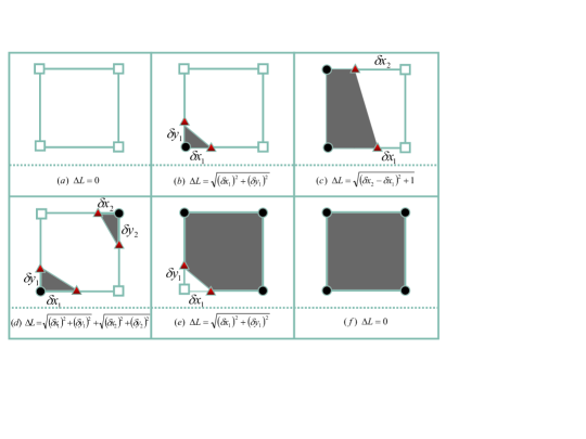
To quantitatively analyse the coupled RTKHI process, we resort to morphological analysis technique. Such a description has been well known in digital picture analysis, and successfully applied to characterize the density, temperature, pressure and particle velocity fields in shocked porous materialsXu et al. (2009), to characterize the spinodal decomposition and domain growth processes in phase separation of multiphase flowsGan et al. (2011, 2012), and to characterize the physical fields in evolution process of KHI systemGan et al. (2019), etc. The basic idea of morphological analysis is as follows. A physical field $\theta(x,y)$ can be defined as two kinds of characteristic regimes: When the physical quantity $\theta(x,y)$ is beyond the threshold value $\theta_{th}$, the grid node at position $(x,y)$ is regarded as a white (or hot) vertex, otherwise it is regarded as a black (or cold) one. A region with connected white or black nodes is defined as a white or black domain. In this way, the continuous image of physical field is converted into a Turing pattern, which is composed of only white and black pixels. For such a Turing pattern, a general theorem of integral geometry states that all the properties of a D-dimensional convex set satisfying motion invariance and additivity are contained in $D+1$ Minkowski measures. To be specific, for a two dimensional field, the three Minkowski measures are the total fractional area $Area$ of the white regimes, the boundary length $L$ between the white and black regimes, and the Euler characteristic $\chi$ describing the connectivity of the domains. When the threshold $\theta_{th}$ is increased from the lowest to the highest values of $\theta(x,y)$ in the system, the white area $Area$ will decrease from 1 to 0; the boundary length $L$ first increases from 0, then arrives at a maximum value, and finally decreases to $0$ again. The Euler characteristic $\chi$ is defined as $\chi=N_{W}-N_{B}$, where $N_{W}$ ($N_{B}$) is the number of connected white (black) domains. The smaller the Euler characteristic $\chi$, the higher the connectivity of the structure with $\theta(x,y)\geq\theta_{th}$ or $\theta(x,y)<\theta_{th}$. A schematic diagram of morphological characterizations is shown in Fig. 1. Figures 1(a) to 1(f) represent different pixel distributions, and the incremental calculations of boundary length in each case are presented. The white squares (black circles) in the figure indicate that the values at these grid points are higher (lower) than the threshold value. The red triangles indicate that the values at the marked positions are equal to the threshold value, and the positions are determined by linear interpolation of the values on adjacent grid points.

In 2010 Xu, et al. Xu et al. (2010) suggested to use the phase space opened by the morphological quantities, $Area$, $L$ and $\chi$, to investigate the morphological property of two dimensional pattern. In such a morphological phase space, one point presents a complete description of the morphological characteristics of the pattern. The less the distance

$$Dist=\sqrt{(Area_{2}-Area_{1})^{2}+(L_{2}-L_{1})^{2}+(\chi_{2}-\chi_{1})^{2}}$$ (10)

between two points, 1 and 2, the higher the similarity of the two corresponding patterns in morphological characteristics. Therefore, the reciprocal of the distance $Dist$ between two points, $1/Dist$, can be defined as a pattern similarity $Sim$ in morphological characteristics, i.e.,

$$Sim=1/Dist.$$ (11)

When the distance $Dist=0$, the similarity $Sim=\infty$, which means the morphological characteristics of the two patterns are the same. Go a further step, if the two patterns evolve with time from $t_{1}$ to $t_{2}$, then we can define a process similarity for the two pattern evolution processes during this period,Xu et al. (2010, 2011, 2016)

$$Sim_{P}=1/Dist_{P},$$ (12)

where

$$Dist_{P}=\frac{1}{{\left({{t_{2}}-{t_{1}}}\right)}}\int\limits_{{t_{1}}}^{{t_{2}}}{{Dist}(t){\rm{}}dt}.$$ (13)

The less the process similarity $Sim_{P}$, the larger the process difference $Dist_{P}$. These concepts and measuring methods have greatly promoted the development of physical cognition in related fields, such as phase separation, KH instability, shock wave kinetics of heterogeneous materials, etc.Xu et al. (2010, 2011, 2016). In this work, we checked and found that, among the three morphological quantities, the boundary length $L$ perform the best in describing the evolution process of perturbed interface and the degree of material mixing. We will focus only on the behavior of $L$. Therefore, in this work,

$$Dist=\sqrt{(L_{2}-L_{1})^{2}}.$$ (14)

III Numerical Simulations

The multiple-relaxation-time DBM model has been validated by some well-known benchmark tests, and satisfying agreements are obtained between the simulation results and analytical onesChen, Xu, and Zhang (2016, 2018). In this section, we investigate the coupled RTI and KHI system with this model; morphological and non-equilibrium analysis are also introduced to probe the complex process. We work in a frame where the gas constant $R=1$.

The initial macroscopic quantities in this study are given as follows:

$$T(y)=T_{u},\;\rho(y)=\rho_{u}\exp(-g(y-y_{s})/T_{u}),$$ (15)

$$u_{x}(y)=u_{0},\;u_{y}(y)=0, \text{for }y\geq y_{s},$$

$$T(y)=T_{b},\;\rho(y)=\rho_{b}\exp(-g(y-y_{s})/T_{b}),$$

$$\;u_{x}(y)=-u_{0},\;u_{y}(y)=0, \text{for }y<y_{s},$$

where $y_{s}=40+2\cos(0.1\pi x)$ denotes the interface with initial small perturbation. The computational domain is a two-dimensional box with height $H=80$ and width $W=20$. To be at equilibrium, the same pressure at the interface is required:

$$p_{0}=\rho_{u}T_{u}=\rho_{b}T_{b},$$ (16)

where $T_{u}<T_{b}$ and $\rho_{u}>\rho_{b}$. To have a finite width of the initial interface, all numerical experiments are performed by preparing the initial configuration plus a smooth interpolation between the two half-volumes. The initial temperature profile is therefore chosen to be

$$T(y)=(T_{u}+T_{b})/2+(T_{u}-T_{b})/2\times\tanh((y-y_{s})/w),$$ (17)

where $w$ denotes the initial width of the interface. The initial density $\rho(y)$ is then fixed by the initial settings (Eqs. (15)–(16)) combined with the smoothed temperature profile. In the simulation, the bottom and the top boundaries are solid wall, the left and right boundaries are periodic boundary conditions. Time discretization is performed with a third-order Runge-Kutta scheme, and the fifth-order weighted essentially non-oscillatory (WENO) scheme is adopted for space discretization. The amplitude $A$ of pure RTI is often defined as half of the maximum distance between the the tips of bubble and spike. For the sake of contrast, the amplitudes of pure RTI, pure KHI and RTKHI systems are defined as half of the mixing width.

III.1 Morphological analysis of pure RTI and pure KHI systems

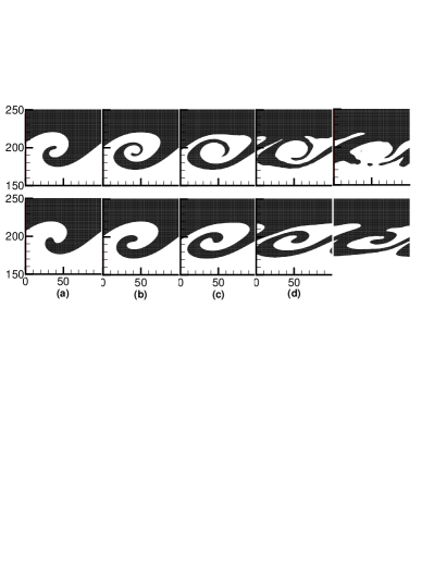
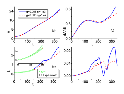
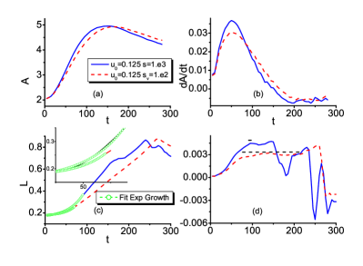
For comparison, we first simulate the pure RTI and the pure KHI systems. Figures 2 and 3 show the temperature Turing patterns of pure RTI ($g=0.005$, $u_{0}=0$) and pure KHI ($g=0$, $u_{0}=0.125$) at times $t=100,150,200,250,300$, respectively. The threshold value is $T_{th}=1.0$. In Figure 2, the left and right sides of each subgraph correspond to $s_{v}=10^{3}$ and $s_{v}=10^{2}$ (with other collision parameters being $10^{3}$), respectively. In Fig. 3, the upper and lower lines correspond to the simulation results of $s_{v}=10^{3}$ and $s_{v}=10^{2}$ (with other collision parameters being $10^{3}$), respectively. The initial conditions and parameters are set as: $\rho_{b}=1$, $T_{b}=1.4$, $\rho_{u}=2.33333$, $T_{u}=0.6$, $w=0.8$, $\gamma=1.4$, $c=1$, $\eta_{0}=3$, $dx=dy=0.2$, $dt=10^{-3}$.

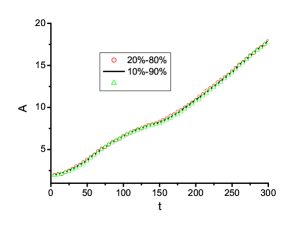
In many experimental studies of coupled RTKHI, $5\%$ and $95\%$ (or $10\%$ and $90\%$) volume fraction points (with respect to bottom stream fluid) are often chosen as the criterion to locate these upper and lower edges, respectively, in order to calculate the mixing width. This criterion has been justified by Snider and Andrews in 1994 and used in many work Akula, Andrews, and Ranjan (2013); Akula and Ranjan (2016); Akula et al. (2017). In our numerical experiment, the temperature of the light fluid at the bottom is $1.4$, and the temperature of the heavy fluid at the top is $0.6$. The $\tanh$ function is used for smooth transition at the interface, as shown in Eq. (17). So, in our morphological analysis, the range of temperature $T$ is $0.6\leq T\leq 1.4$. Within this range, the $10\%$ and $90\%$ correspond to $T=0.68$ and $T=1.32$, respectively, which are chosen as the criterion to locate these upper and lower edges to calculate the mixing width. In Fig. 4, the amplitude curves obtained by using different criterions for the case ($g=0.005$ and $u_{0}=0.1$) are shown. The black solid line corresponds to $10\%-90\%$ criterion, the red circles correspond to $20\%-80\%$ criterion, and the green triangles correspond to $5\%-95\%$ criterion. These results are in good agreement. Figures 5 and 6 show the time evolutions of amplitude $A$ and the morphological boundary length $L$ with threshold $T_{th}=1.0$ of the pure RTI and KHI, respectively.

Figure 2: Temperature Turing patterns of pure RTI ($g=0.005$, $u_{0}=0$, $T_{th}=1.0$). (a), (b), (c), (d) and (e) correspond to $t=100,150,200,250,300$. The left and right sides of each subgraph correspond to $s_{v}=10^{3}$ and $s_{v}=10^{2}$, respectively.

Figure 3: Temperature Turing patterns of pure KHI ($g=0$, $u_{0}=0.125$, $T_{th}=1.0$). (a), (b), (c), (d) and (e) correspond to $t=100,150,200,250,300$. The upper and lower lines correspond to $s_{v}=10^{3}$ and $s_{v}=10^{2}$, respectively.

Figure 4: Calculation of the amplitude $A$ for the case ($g=0.005$ and $u_{0}=0.1$).

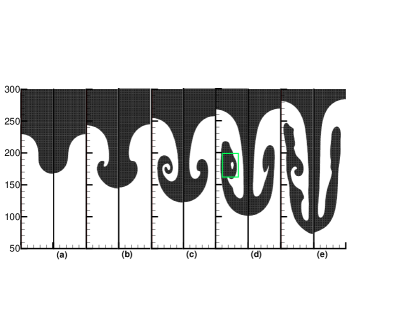
In the evolution of pure RTI (as shown in Figs. 2, 5(a) and 5(b)), the perturbation amplitude is initially much smaller than the wave length, and the perturbation increases exponentially; as the light density (hot) and heavy density (cold) fluids gradually penetrate into each other, an obvious bubble-spike structure is gradually formed, the amplitude transitions from exponential growth to linear growth with time; subsequently, the top of the spike forms a mushroom-shaped structure due to the KHI, and the amplitude growth rate decreases slightly at this time; at a later time, extrusion from the two sides leads to the formation of secondary spikes, and the growth rate increases again (reacceleration stage). For fixed initial conditions and model parameters, high viscosity suppresses the development of RTI by inhibiting the development of KHI on the two sides of the spike.

In the evolution of pure KHI (as shown in Fig. 3), under the action of initial perturbation and tangential velocity, the perturbation gradually grows to a sinuous structure, and then a rolled-up vortex (Figs. 3(a)-3(c)). In the final, the normal vortex structure collapses to nonregular structures and the system develops to the turbulent stage (Fig. 3(e)). Keeping other conditions and settings unchanged, the larger the viscosity is, the weaker the KHI will be, and the later the vortex formulates and collapses.

Figure 5: The pure RTI, (a) amplitude $A$, (b) growth rate of amplitude $dA/dt$, (c) morphological boundary length $L$ of the temperature field, (d) growth rate of boundary length $dL/dt$.

Figure 6: The pure KHI, (a) amplitude (1/2 width of the mixing layer) $A$, (b) growth rate of amplitude $dA/dt$, (c) morphological boundary length $L$ of the temperature field, (d) growth rate of boundary length $dL/dt$.

Compared with the commonly used descriptions of amplitude and amplitude growth rate, the morphological boundary length $L$ can analyze the development of instability system from different angles.

i) We first compare the blue curves of amplitude and morphological boundary length of pure RTI in the case of $s_{v}=10^{3}$ in Fig. 5. The amplitude shows a smooth rising curve, and the amplitude growth rate increases rapidly at $t=250$, indicating that the system has entered the reacceleration stage. However, a small platform appears on the morphological boundary length $L$ at this time. The platform is a result of two factors: first, the continuous development of RTI increases $L$ (factor 1), and second, the destruction of the KHI vortex structure on both sides of the mushroom (marked by the green box in Fig. 2(d)) reduces $L$ (factor 2). The two factors cancel each other. With the increasing viscosity, the boundary length $L$ decreases, and the degree of material mixing decreases. In addition, due to the suppression effect of viscosity, the effect of factor 2 just mentioned above is weakened, making the platform approximately disappear (red curve in Fig. 5(c)).

ii) In Fig. 6, before the fully developed turbulence stage, both the Mixing layer width and the boundary length $L$ of KHI increase at first, and then decreases, and the viscosity delays the appearance of the peak. When the Mixing layer width reaches the maximum, the vortex structure continues to develop, and the morphological boundary length $L$ continues to increase. The inflection points at which $L$ decreases (at times $t=240$ and $270$) mean that the overall structure of the KHI vortex begins to break (as shown in Figs. 3(d) and 3(e)).

iii) Comparing the boundary length and its growth rate curves of RTI and KHI, it is found that, after the initial exponential growth stage, the boundary length of KHI has a constant velocity growth stage (marked with blue dotted lines), which is different from RTI, and the increase in viscosity helps to extend this process.

III.2 Morphological analysis of Coupled RTKHI systems

In this section, we use morphological description to study the coupled RTKHI. Figures 7, 8, and 9 show the temperature images and the corresponding Turing patterns of different RTKHI systems.

Figure 7: A coupled RTKHI with $g=0.005$ and $u_{0}=0.05$. (a) and (b) are the temperature and the corresponding Turing pattern ($T_{th}=1.0$) of the RTKHI, respectively. (c) is temperature Turing pattern of pure KHI with $u_{0}=0.05$. The images from left to right correspond to $t=100,150,200,250,300$, respectively. All figures in the first line follow the same legend.

Figure 8: A coupled RTKHI with $g=0.005$ and $u_{0}=0.1$. (a) and (b) are the temperature and the corresponding Turing pattern ($T_{th}=1.0$) of the RTKHI, respectively. (c) is temperature Turing pattern of pure KHI with $u_{0}=0.1$. The images from left to right correspond to $t=100,150,200,250,300$, respectively. All figures in the first line follow the same legend.

Figure 9: A coupled RTKHI with $g=0.005$ and $u_{0}=0.15$. (a) and (b) are the temperature and the corresponding Turing pattern ($T_{th}=1.0$) of the RTKHI, respectively. (c) is temperature Turing pattern of pure KHI with $u_{0}=0.15$. The images from left to right correspond to $t=100,150,200,250,300$, respectively. All figures in the first line follow the same legend.

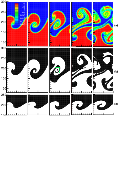
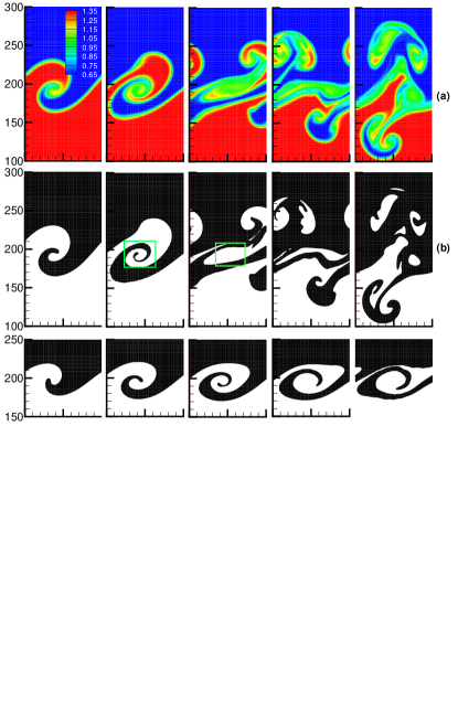
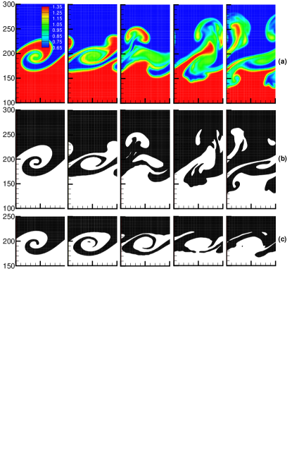
Figure 7 corresponds to the case of $g=0.005$, $u_{0}=0.05$ (case 1). Compared with the pure RTI Turing patterns ($g=0.005$, Fig.2), and the pure KHI Turing patterns ($u_{0}=0.05$, Fig. 7(c)), it can be found that, the oblique and asymmetric bubbles, spikes and even mushroom-like structures are shown from beginning to end in Figs. 7(a) and 7(b), and the evolution of pure KHI in Fig. 7(c) lags far behind that in Fig. 7(b). Therefore, the RTI plays a major role, although KHI always exists in this system. The existence of shear velocity is mainly to destroy the symmetry of the RTI structure.

Figure 8 corresponds to the case of $g=0.005$, $u_{0}=0.1$ (case 2). It can be found that, the interface and vortex growth of the RTKHI system, shown in Figs. 8(a) and 8(b), show similar magnitudes to those of the pure RTI, shown in Fig. 2 and the pure KHI with $u_{0}=0.1$, shown in Fig. 8(c), before the time $t=150$. In this process, neither RTI nor KHI can be ignored. After the time $t=150$, the vortex structure of the system is destroyed (marked by the green boxes in Fig. 8(b)), and an asymmetric mushroom-like structure (representative structure of RTI) is also generated. At this time, RTI plays a major role.

Figure 9 corresponds to the case of $g=0.005$, $u_{0}=0.15$ (case 3). The spanwise vortical structures which are characteristic of free shear flows are clearly seen at earlier time ($t<=100$), so KHI plays a major role at the initial stage. As time progresses, more fluid is entrained in the vortical structure, and the secondary RTI develops rapidly along the vortex arms ($t=150$). Subsequently, the vortex structure of KHI is quickly stretched and diffused, and RTI drives the mixing layer growth ($t=200$). In the later turbulence stage, the combined effect of gravity acceleration and shear makes the interface more irregular ($t=250,300$).

Figure 10: Perturbation amplitude $A$, growth rate $dA/dt$, and morphological boundary length $L$ versus time $t$. For convenience of comparison, the results for the coupled RTKHI, pure RTI and pure KHI systems are presented in different form of graph. Figures (a) and (b) show the perturbation $A$ and morphological boundary length $L$ for various cases, including the coupled RTKHI, the pure RTI and pure KHI. In Figs. (c), (d) and (e), the evolution of three quantities, $A$, $dA/dt$, and $L$, are shown in the same graph for one case of RTKHI system. The shear rates in (c), (d) and (e) are $u_{0}=0.2$, $u_{0}=0.15$, $u_{0}=0.125$, respectively. The black, red and green solid lines represent the amplitude, amplitude growth rate and boundary length of the RTKHI system, respectively. For comparison, the amplitude $A$ of the corresponding pure KHI is also plotted by black dashed line in Figs. (c), (d) and (e).

Figure 11: Morphological analysis of the main mechanism in the early stage. Figures (a) and (b) show the comparison of boundary length $L$ between pure RTI and different pure KHI. The small insets in the middle column are the temperature Turing patterns of pure RTI (corresponding to black curves in (a) and (b)) and the corresponding pure KHI (corresponding to green curves in (a) and (b)) at the times marked by the intersection points, P₁ and P₃ in (a) and (b). (c) and (d) shows the linear relationships between gravity acceleration $g$ and critical shear velocity $u_{C}$, gravity acceleration $g$ and Reynolds number $Re$. The regions for KHI or RTI dominates are obtained.

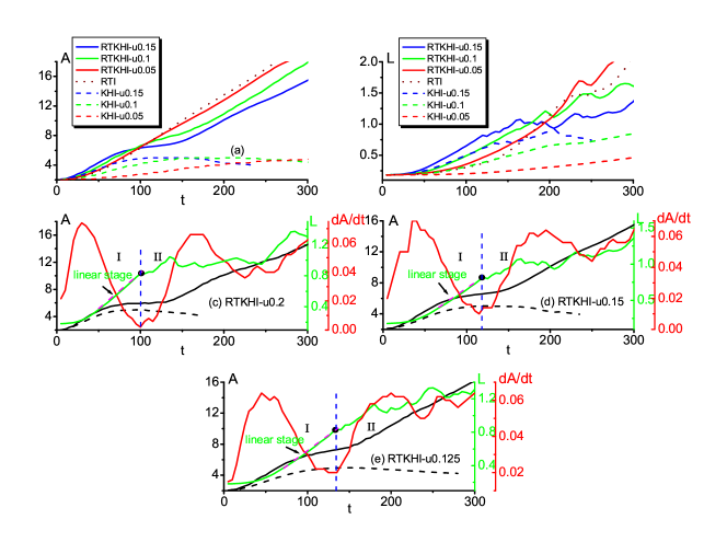
Next, the focus of our work shifts to two judgments: i) Qualitatively speaking, for the early stage of the coupled RTKHI system, when the shear effect is relatively small, RTI dominates; when the shear is relatively large, KHI will play a major role. How to judge quantitatively ? ii) For the case where the KHI dominates at earlier time and the RTI dominates at later time, how to judge this transition point from KHI-like to RTI-like. It is important to quantify these transition points for different cases and determine any criterion for transition.

In Fig. 10, perturbation amplitude $A$, growth rate $dA/dt$, and morphological boundary length $L$ versus time $t$ are shown. For convenience of comparison, the results for the coupled RTKHI, pure RTI and pure KHI systems are presented in different form of graph. Figures 10(a) and 10(b) show the perturbation $A$ and morphological boundary length $L$ for various cases, including the coupled RTKHI, the pure RTI and pure KHI. In Figs. 10 (c), (d) and (e), the evolution of three quantities, $A$, $dA/dt$, and $L$, are shown in the same graph for one case of RTKHI system. The shear rates in 10(c), (d) and (e) are $u_{0}=0.2$, $u_{0}=0.15$, $u_{0}=0.125$, respectively. The black, red and green solid lines represent the amplitude, amplitude growth rate and boundary length of the RTKHI system, respectively. For comparison, the amplitude $A$ of the corresponding pure KHI is also plotted by black dashed line in each of Figs. 10(c), (d) and (e). The superposition of shear on RTI increases the mixing width and boundary length at early time, while this effect is not observed at later time. The morphological boundary length curves are complicated and variable in the later time, and these complicated changes are due to the development and deformation of the vortex, and the coalescence of the hot and cold domains. The amplitude curves show that the system has a growth trend similar to pure RTI in the later stage, and verify the qualitative description mentioned above again. For the case where the KHI dominates at earlier time and the RTI dominates at later time, the evolution process can be roughly divided into two stages, that is, shear dominance stage and buoyancy dominance stage. The state of transition from shear dominance to buoyancy dominance is called the transition point. As can be seen from the figure, in the initial stage, $L^{RTKHI}$ initially increases exponentially, and then increases linearly (purple dashed lines). The ending point of linear increasing $L^{RTKHI}$ is approximately equal to the minimum point of amplitude growth rate $dA/dt$ of the RTKHI system, and the maximum point of amplitude $A$ of the corresponding pure KHI system. From this moment, the RTI begins to play a major role. This moment is referred to as the transition point, which is marked by a dashed vertical line and circle in each figure. Hence, the ending point of linear increasing $L^{RTKHI}$ can work as a geometric criterion for discriminating the two stages. The higher the shear rate is, the earlier the transition appears.

We also calculate the Richardson number $R_{i}$ corresponding to the transition point, based on the following equationAkula, Andrews, and Ranjan (2013); Akula et al. (2017); Finn (2014),

$$R_{i}=\frac{-g(\partial\rho/\partial y)}{\rho(\partial u/\partial y)^{2}}\thickapprox-\frac{2hg\Delta\rho}{\rho(\Delta U)^{2}}=-\frac{4ghAt}{(\Delta U)^{2}}\text{,}$$ (18)

where $2h$ signifies the width of the mixing layer, $\Delta\rho$ and $\Delta U$ are the differences in density and velocity, $\rho$ is the average density, $At$ is the Atwood number, $At=(\rho_{u}-\rho_{b})/(\rho_{u}+\rho_{b})=\Delta\rho/(2\rho)$. For the cases of 10(c), 10(d), and 10(e), the corresponding values are obtained $R_{ic}=-0.295$, $R_{id}=-0.587$, $R_{ie}=-0.9344$. The smaller the negative $Ri$ is, the stronger the effect of shear will be. The results show a satisfactory agreement with the work by Finn Finn (2014).

Then, we focus our attention on the early stage of the RTKHI system. In the RTKHI system, RTI always plays a major role in the later stage, while the main mechanism in the early stage depends on the comparison of buoyancy and shear strength (namely, the gravity acceleration $g$ and the shear velocity $u_{0}$). That is, both types of instability develop with time, however, as there are differences between powerful and weak strength, there will be the primary one as well as secondary one. For a given gravity acceleration $g$, there is a critical shear velocity $u_{C}$. In the corresponding coupling system with gravity acceleration $g$ and shear velocity $u_{C}$, the buoyancy and shear effects are balanced. If the shear velocity $u_{0}$ of the RTKHI system is greater than $u_{C}$, the shearing effect in the early stage of the system is stronger, and consequently the KHI dominates in the early stage (as shown in Fig. 9); If the shear velocity $u_{0}$ of the RTKHI system is less than $u_{C}$, the shearing effect is weaker, and consequently the RTI dominates in the early stage (as shown in Fig. 7).

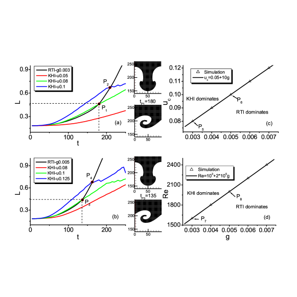
Figure 11 shows the morphological analysis of the main mechanism in the early stage. Figures (a) and (b) are comparisons of the boundary lengths of pure RTI and different pure KHI. The small insets in the middle column are the temperature Turing patterns of pure RTI (corresponding to black curves in (a) and (b)) and the corresponding pure KHI (corresponding to green curves in (a) and (b)) at the times marked by the intersection points, P₁ and P₃ in (a) and (b). For the convenience of description, we use the pair of typical parameters ($g$, $u_{0}$) to label the corresponding pair of systems/process. In Figs. (a) and (b), for the pure KHI system/process, the boundary length $L$ increases with the increasing shear velocity $u_{0}$ during the initial period. In Fig.(a), the boundary lengths of the pure RTI system with $g=0.003$ (black line) and the pure KHI system with the shear velocity $u_{0}=0.08$ (green line) keep close before the time $t=180$ at which the two curves intersect at point P₁, which means that, $L^{RTI}=L^{KHI}$, $Dist=\left|L^{RTI}-L^{KHI}\right|=0$, the pattern similarity $Sim=\infty$ at this moment. During the period $0\leq t\leq 180$, the process similarity $Sim_{P}$ keeps nearly $\infty$. That is to say, the two systems/processes have the same degree of material mixing at this moment and keep nearly the same degree of material mixing before this moment from this perspective. The $L$ curve for the pure KHI with $u_{0}=0.05$ (red line) is below the $L$ curve of the pure RTI system with $g=0.003$ (black line), and the two $L$ curves deviate more with time. That is to say, the process similarity $Sim_{P}$ of the pair of systems/processes decreases with time. It is shown that the $L$ curve for the pure KHI with $u_{0}=0.1$ (blue line) and the $L$ curve for the pure RTI with $g=0.003$ (black line) intersects also at the point P₂. It should be pointed out that, even though $L^{RTI}=L^{KHI}$, $Dist=\left|L^{RTI}-L^{KHI}\right|=0$, the pattern similarity $Sim=\infty$ at the moment corresponding to P₂, but it is clear that the process similarity of this pair of systems/processes before the point p₂, $Sim_{P}$, is much less than that of the pair, ($g=0.003$, $u_{0}=0.08$ ). Our numerical results show that, compared with the pure RTI with $g=0.003$, for the pure KHI cases, the one with $u_{0}=0.08$ is the critical case which shows the highest process similarity $Sim_{P}$, the larger the deviation $|u_{0}-0.08|$, the higher the process difference $1/Sim_{P}$, the less the process similarity $Sim_{P}$. Therefore, we refer $u_{0}=0.08$ as to the critical shear velocity $u_{C}$ for $g=0.003$, i.e., $u_{C}(g=0.003)=0.08$. This is what the point P₅ in Fig. (c) means. Figure (b) shows a second set of numerical results which can be interpreted in the same way. Figure (b) shows that, compared with the pure RTI with $g=0.005$, for the pure KHI cases, the one with $u_{0}=0.1$ is the critical case which shows the highest process similarity $Sim_{P}$, i.e., $u_{C}(g=0.005)=0.1$. This is what the point P₆ in Fig. (c) means. The other points in Fig.(c) are obtained in a similar way. It is interesting to find that $u_{C}$ shows a linear relationship with $g$. In the space opened by parameters $g$ and $u_{C}$, in the region above the line KHI dominates the RTKHI system, in the region below the line RTI dominates. If we introduce a Reynolds number $Re$ defined as

$$Re=\rho u_{C}\lambda/\mu$$

the five points in Fig.(c) will be transformed to the five points in Fig. (d), where $\lambda$ is taken as the initial wavelength of interface perturbation, the coefficient of viscosity is $\mu=\rho T/s_{v}$, and $T$ is taken as the average temperature, $T=1.0$. Figure (d) shows the parameter regions where KHI dominates and RTI dominates in the space opened by Reynolds number $Re$ and gravity $g$.

Therefore, the value of morphological total boundary length $L$ is an helpful and efficient indication for the degree of instability development or material mixing. Furthermore, $L$ of the condensed temperature field can be used to measure the ratio of buoyancy to shear strength, and consequently it can be used to quantitatively judge the main mechanism in the early stage of the RTKHI system. Specifically, when KHI (RTI) dominates, $L^{KHI}>L^{RTI}$ ($L^{KHI}<L^{RTI}$); when KHI and RTI are balanced, $L^{KHI}=L^{RTI}$.

In addition, it should be noted that the points (the intersections of the $L$ curves of pure KHI and RTI) in Figs. 11(a) and (b) are not the transition points of RTKHI systems. The concept of transition point only exists in the RTKHI system ($u_{0}>u_{C}$) in which KHI plays a major role in the early stage and RTI plays a major role in the later stage. For this type of system, although KHI plays a major role in the early stage, buoyancy always exists. The combined effect of buoyancy and shear will inevitably lead to more rapid development of instability than the pure KHI or RTI system. As a result, the transition point is earlier than the intersections of the $L$ curves in Fig. 11. When the gravitational acceleration is constant, the greater the shear rate, the earlier the transition point appears, as shown in Figs. 10 (c), (d) and (e).

III.3 Non-equilibrium characteristics of RTKHI systems

The system with hydrodynamic instability is a typical non-equilibrium flow system. Therefore, it makes sense to fully understand the various non-equilibrium behavior characteristics within such a system. In this section, the non-equilibrium characteristics of the RTKHI will be discussed. In the evolution of hydrodynamic instability, the non-equilibrium effects are significant near the interface, and basically $0$ in the position far from interface. Figure 12 shows the contours of the non-equilibrium components $\Delta_{(3,1)x}^{\ast}$ (a), $\Delta_{(3,1)y}^{\ast}$ (b) and the corresponding NOEF strength $d_{(3,1)}$ (c) at $t=150$ and $t=250$. $\Delta_{(3,1)x}^{\ast}$ and $\Delta_{(3,1)y}^{\ast}$ correspond to the heat flux in $x$ direction and $y$ direction, respectively. From Figs. 12(a) and (b), it can be found that the negative heat flux and the positive heat flux appear alternately. The closer to the center of the spiral interface, the weaker of the non-equilibrium quantities. In Fig. 12(c), a clear double spiral structure can be seen from $d_{(3,1)}$. These information and structures cannot be found (or are not easy to be found) from the contours of temperature (as shown in Fig.8(a)). Compared with the individual components, the NOEF strength $d_{(3,1)}$ provides a high resolution interface, and can be well used to describe the complete outline of interface in the RTKHI simulation.

Figure 12: Non-equilibrium characteristics of RTKHI system ($g=0.005$, $u_{0}=0.1$), (a) $\Delta_{(3,1)x}^{\ast}$, (b) $\Delta_{(3,1)y}^{\ast}$, and (c) $d_{(3,1)}$. The first and second lines correspond to $t=150$ and $t=250$, respectively. Each column follows the same legend.

Figure 13: The applications of non-equilibrium characteristics in the early main mechanism judgment (a)-(d) and transition point capture (e)-(f). Figs. (a) and (c) show the comparison of global average TNE strength $D_{TNE}$ between pure RTI and different pure KHI. Figs. (b) and (d) show the comparison of global average NOEF strength $D_{3,1}$ between pure RTI and different pure KHI. In Figs. (e) and (f), the evolutions of $L$ and $D_{3,1}$ are shown in the same graph for one case of RTKHI system. The shear rates in (e) and (f) are $u_{0}=0.15$ and $u_{0}=0.2$, respectively.

Figure 14: The linear relationship between $L$ and $D_{3,1}$ in the early stage. Figs. (a) and (b) show the effects of viscosity and heat conductivity. The relations between intercept and slope of linear fitting shown in Fig. (b) and heat conductivity are shown in Figs. (c) and (d), respectively.

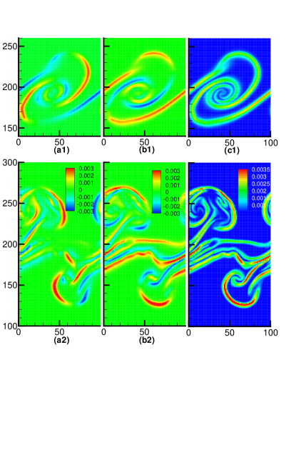
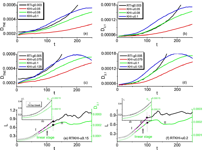
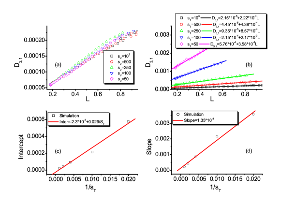
Figure 13(a)-(d) shows the applications of non-equilibrium characteristics in the early main mechanism judgment. Compared with the global average TNE strength $D_{TNE}$ shown in 13(a) and (c), the global average NOEF strength $D_{3,1}$ shown in 13(b) and (d) can more accurately judge the main mechanism in the early stage, and the conclusions are consistent with the morphological boundary length $L$ (as shown in figure 11). Specifically, when KHI (RTI) dominates in the early RTKHI system, $D_{3,1}^{KHI}>D_{3,1}^{RTI}$ ($D_{3,1}^{KHI}<D_{3,1}^{RTI}$); when KHI and RTI are balanced, $D_{3,1}^{KHI}=D_{3,1}^{RTI}$. The global average TNE strength $D_{TNE}$ cannot be used as the distinguish criterion, because the global average TNE strength is closely related to density nonuniformity, and the initial density of RTI is a function of acceleration $g$, which is completely different from the density setting of KHI.

Since morphologic quantities and non-equilibrium quantities describe the same physical process from different perspectives, there must be a relationship between them. It is worth studying which quantities are strongly correlated and which are weakly correlated. This is the core task of several of our previous work Chen, Xu, and Zhang (2016, 2018). In our previous work Chen, Xu, and Zhang (2016, 2018) we have make it clear that the mean Non-Organized Energy Flux (NOEF) $D_{3,1}$ and mean temperature nonuniformity has a high correlation which is almost 1. How does the specific correlation behavior between the total boundary length $L$ and $D_{3,1}$ naturally becomes an interesting question. In figures 13(e) and 13(f), $D_{3,1}$ shows similar behavior to the boundary length $L$. We adopt the correlation function $C$ to express this similarity.

$$C=\frac{\overline{(L-\overline{L})(D_{3,1}-\overline{D_{3,1}})}}{\sqrt{\overline{(L-\overline{L})^{2}}\cdot\overline{(D_{3,1}-\overline{D_{3,1}})^{2}}}}$$ (19)

where $\overline{L}$ and $\overline{D_{3,1}}$ are the averages of $L$ and $D_{3,1}$ in the time concerned, respectively. It is interesting to find that the two quantities, $L$ and $D_{3,1}$, always show a high correlation, especially in the early stage (This finding also exists in pure RT and pure KH systems). In figure 13(e) (13(f)), the overall correlation degrees between $D_{3,1}$ and $L$ is approximate to $0.985$ ($0.967$), the correlation in the early stage (stage I) is $0.999$ ($0.999$), and it decrease to $0.716$ ($0.269$) in the later stage (stage II). The physical reason is as below. $D_{3,1}$ is the mean heat flux strength, which is closely related to temperature gradient. The macroscopic quantity gradient, especially the temperature gradient, mainly exists near the interface. The greater the interface length $L$ is, the larger $D_{3,1}$ is. Therefore, $D_{3,1}$ can also be used to capture the transition points from KHI-like to RTI-like (as shown by the black vertical lines in figures 13(e) and 13(f)). When $D_{3,1}$ deviates from its constant velocity growth, the system enters the second stage. That is, the ending point of linear increasing $D_{3,1}$ can work as a physical criterion for discriminating the two stages.

The high correlation between $L$ and $D_{3,1}$ in the early stage means that $L$ and $D_{3,1}$ follows roughly a linear relationship. Figure 14 shows the linear relationship between $L$ and $D_{3,1}$ in the early stage, where Figs. 14(a) and (b) are the effects of viscosity and heat conduction, respectively. The solid lines are linear fittings corresponding to the simulation results. It can be seen that heat conduction has a significant influence on the linear relationship. With the increase of heat conduction, the intercepts and slopes of the linear relationship increase approximately linearly (Figs. 14(c) and (d)).

IV Conclusions

In this paper, we investigate the coupled Rayleigh-Taylor-Kelvin-Helmholtz instability system with a multiple-relaxation time discrete Boltzmann model. To quantitatively analyse the coupled RTKHI process, we resort to morphological and non-equilibrium analysis techniques, and three cases are considered: pure RTI, pure KHI, and coupled RTKHI systems. After the initial exponential growth stage, the total boundary length $L$ of the condensed temperature field of pure KHI has an approximately constant velocity growth stage, which is different from the pure RTI. RTI always dominates in the later stage of coupled RTKHI system, while the main mechanism in the early stage depends on the comparison of buoyancy and shear strength. Both the total boundary length $L$ of the condensed temperature field and the mean heat flux strength $D_{3,1}$ can be used to measure the ratio of buoyancy to shear strength, and to quantitatively judge the main mechanism in the early stage of the RTKHI system. Specifically, when KHI (RTI) dominates, $L^{KHI}>L^{RTI}$ ($L^{KHI}<L^{RTI}$), $D_{3,1}^{KHI}>D_{3,1}^{RTI}$ ($D_{3,1}^{KHI}<D_{3,1}^{RTI}$); when KHI and RTI are balanced, $L^{KHI}=L^{RTI}$, $D_{3,1}^{KHI}=D_{3,1}^{RTI}$, where the superscript, “KHI (RTI) " , indicates the type of hydrodynamic instability. It is interesting to find that, (i) for the critical cases where KHI and RTI are balanced, both the critical shear velocity $u_{C}$ and Reynolds number $Re$ show a linear relationship with the gravity/accelaration $g$; (ii) the two quantities, $L$ and $D_{3,1}$, always show a high correlation, especially in the early stage where it is roughly $0.999$, which means that $L$ and $D_{3,1}$ follows approximately a linear relationship. The heat conduction has a significant influence on the linear relationship. For the case where the KHI dominates at earlier time and the RTI dominates at later time, the boundary length $L$ can well capture the transition point from KHI-like to RTI-like. Before the transition point of the two stages, $L^{RTKHI}$ initially increase exponentially, and then increases linearly. This linear increasing behavior ends at the transition point. Hence, the ending point of linear increasing $L^{RTKHI}$ can work as a geometric criterion for discriminating the two stages. The TNE quantity, heat flux strength $D_{3,1}^{RTKHI}$ shows similar behavior to boundary length $L$, and a strong positive correlation can be found in the early stage. Therefore, the ending point of linear increasing $D_{3,1}^{RTKHI}$ can work as a physical criterion for discriminating the two stages. The morphological boundary length $L$ is the length of the interface between light and heavy (high and low temperature) fluids. It reflects the degree of instability development and material mixing. The TNE quantity $D_{3,1}$ reflects the degree of deviation from equilibrium in different regions of the system, and can more clearly and accurately locate the position of the interface. The two criteria, $L$ and $D_{3,1}$, have different perspectives, but are consistent, have their own advantages, and complement each other. The resort to these two criteria facilitates the identification of the main mechanisms and critical time of the coupled RTKHI systems.

Data Availability

The data that support the findings of this study are available from the corresponding author upon reasonable request.

Appendix: Transformation matrix and equilibria of the kinetic moments

The transformation matrix and the corresponding equilibrium distribution functions in KMS are constructed according to the seven moment relations. Specifically, the transformation matrix is

$$\mathbf{M}=(m_{1},m_{2},\cdots,m_{16})^{T}\text{,}\;$$

$$m_{1}=1\text{,}\;m_{2}=v_{ix}\text{,}\;m_{3}=v_{iy}\text{,}\;m_{4}=(v_{i\alpha}^{2}+\eta_{i}^{2})/2\text{,}\;$$

$$m_{5}=v_{ix}^{2}\text{,}\;m_{6}=v_{ix}v_{iy}\text{,}\;m_{7}=v_{iy}^{2}\text{,}\;$$

$$m_{8}=(v_{i\beta}^{2}+\eta_{i}^{2})v_{ix}/2\text{,}\;m_{9}=(v_{i\beta}^{2}+\eta_{i}^{2})v_{iy}/2\text{,}\;$$

$$m_{10}=v_{ix}^{3}\text{,}\;m_{11}=v_{ix}^{2}v_{iy}\text{,}\;m_{12}=v_{ix}v_{iy}^{2}\text{,}\;m_{13}=v_{iy}^{3}\text{,}\;$$

$$m_{14}=(v_{i\chi}^{2}+\eta_{i}^{2})v_{ix}^{2}/2\text{,}\;m_{15}=(v_{i\chi}^{2}+\eta_{i}^{2})v_{ix}v_{iy}/2\text{,}\;$$

$$m_{16}=(v_{i\chi}^{2}+\eta_{i}^{2})v_{iy}^{2}/2\text{.}\;$$

The corresponding equilibrium distribution functions in KMS are

$$\hat{f}_{1}^{eq}=\rho\text{,}\;\hat{f}_{2}^{eq}=\rho u_{x}\text{,}\;\hat{f}_{3}^{eq}=\rho u_{y}\text{,}\;\hat{f}_{4}^{eq}=e\text{,}\;$$

$$\hat{f}_{5}^{eq}=P+\rho u_{x}^{2}\text{,}\;\hat{f}_{6}^{eq}=\rho u_{x}u_{y}\text{,}\;\hat{f}_{7}^{eq}=P+\rho u_{y}^{2}\text{,}\;$$

$$\hat{f}_{8}^{eq}=(e+P)u_{x}\text{,}\;\hat{f}_{9}^{eq}=(e+P)u_{y}\text{,}\;\hat{f}_{10}^{eq}=\rho u_{x}(3T+u_{x}^{2})\text{,}\;$$

$$\hat{f}_{11}^{eq}=\rho u_{y}(T+u_{x}^{2})\text{,}\;\hat{f}_{12}^{eq}=\rho u_{x}(T+u_{y}^{2})\text{,}\;\hat{f}_{13}^{eq}=\rho u_{y}(3T+u_{y}^{2})\text{,}\;$$

$$\hat{f}_{14}^{eq}=(e+P)T+(e+2P)u_{x}^{2}\text{,}\;\hat{f}_{15}^{eq}=(e+2P)u_{x}u_{y}\text{,}$$

$$\hat{f}_{16}^{eq}=(e+P)T+(e+2P)u_{y}^{2}\text{,}$$

where pressure $P=\rho RT$ and energy $e=b\rho RT/2+\rho u_{\alpha}^{2}/2$. $R$ is the specific gas constant and $b$ is a constant related to the specific-heat-ratio $\gamma$ by $\gamma=(b+2)/b$.

Replacing $v_{i\alpha}$ by $v_{i\alpha}-u_{\alpha}$ in the transformation matrix $\mathbf{M}$, matrix $\mathbf{M}^{\ast}$ is expressed as follows:

$$\mathbf{M}^{\ast}=(m_{1}^{\ast},m_{2}^{\ast},\cdots,m_{16}^{\ast})^{T},$$

$$m_{1}^{\ast}=1\text{,}\;m_{2}^{\ast}=v_{ix}-u_{x}\text{,}\;m_{3}^{\ast}=v_{iy}-u_{y}\text{,}$$

$$m_{4}^{\ast}=((v_{ix}-u_{x})^{2}+(v_{iy}-u_{y})^{2}+\eta_{i}^{2})/2\text{,}$$

$$m_{5}^{\ast}=(v_{ix}-u_{x})^{2}\text{,}\;m_{6}^{\ast}=(v_{ix}-u_{x})(v_{iy}-u_{y})\text{,}\;m_{7}^{\ast}=(v_{iy}-u_{y})^{2}\text{,}$$

$$m_{8}^{\ast}=[(v_{ix}-u_{x})^{2}+(v_{iy}-u_{y})^{2}+\eta_{i}^{2}](v_{ix}-u_{x})/2\text{,}$$

$$m_{9}^{\ast}=[(v_{ix}-u_{x})^{2}+(v_{iy}-u_{y})^{2}+\eta_{i}^{2}](v_{iy}-u_{y})/2\text{,}$$

$$m_{10}^{\ast}=(v_{ix}-u_{x})^{3}\text{,}\;m_{11}^{\ast}=(v_{ix}-u_{x})^{2}(v_{iy}-u_{y})\text{,}$$

$$m_{12}^{\ast}=(v_{ix}-u_{x})(v_{iy}-u_{y})^{2}\text{,}\;m_{13}^{\ast}=(v_{iy}-u_{y})^{3}\text{,}$$

$$m_{14}^{\ast}=[(v_{ix}-u_{x})^{2}+(v_{iy}-u_{y})^{2}+\eta_{i}^{2}](v_{ix}-u_{x})^{2}/2\text{,}$$

$$m_{15}^{\ast}=[(v_{ix}-u_{x})^{2}+(v_{iy}-u_{y})^{2}+\eta_{i}^{2}](v_{ix}-u_{x})(v_{iy}-u_{y})/2\text{,}$$

$$m_{16}^{\ast}=[(v_{ix}-u_{x})^{2}+(v_{iy}-u_{y})^{2}+\eta_{i}^{2}](v_{iy}-u_{y})^{2}/2.$$

References

- Faganello, Califano, and Pegoraro (2008) M. Faganello, F. Califano, and F. Pegoraro, “Competing mechanisms of plasma transport in inhomogeneous configurations with velocity shear: The solar-wind interaction with earth’s magnetosphere,” Phys. Rev. Lett. 100, 015001 (2008).
- Lawrence, Browand, and Redekopp (1991) G. A. Lawrence, F. K. Browand, and L. G. Redekopp, “The stability of a sheared density interface,” Phys. Fluids A 3, 2360–2370 (1991).
- Yamamoto (2008) T. Yamamoto, “A linear analysis of the hybrid Kelvin-Helmholtz/Rayleigh-Taylor instability in an electrostatic magnetosphere-ionosphere coupling system,” J. Geophys. Res. 113, A06206 (2008).
- Prajapati et al. (2009) R. Prajapati, D. Soni, R. K. Sanghvi, and R. K. Chhajlani, “Kelvin-Helmholtz and Rayleigh-Taylor instability of two superimposed magnetized fluids with suspended dust particles,” Z. Naturforsch. A: Phys. Sci. 64, 455 (2009).
- Guglielmi, Potapov, and Klain (2010) A. V. Guglielmi, A. S. Potapov, and B. I. Klain, “Rayleigh-Taylor-Kelvin-Helmholtz combined instability at the magnetopause,” Geomagn. Aeronomy 50, 958–962 (2010).
- Wang, Ye, and Li (2010) L. F. Wang, W. H. Ye, and Y. J. Li, “Combined effect of the density and velocity gradients in the combination of Kelvin-Helmholtz and Rayleigh-Taylor instabilities,” Phys. Plasmas 17, 042103 (2010).
- Ye et al. (2011) W. H. Ye, L. F. Wang, C. Xue, Z. F. Fan, and X. T. He, “Competitions between Rayleigh-Taylor instability and Kelvin-Helmholtz instability with continuous density and velocity profifiles,” Phys. Plasmas 18, 022704 (2011).
- Mandal et al. (2011) L. Mandal, S. Roy, R. Banerjee, M. Khan, and M. R. Gupta, “Evolution of nonlinear interfacial structure induced by combined effect of Rayleigh-Taylor and Kelvin-Helmholtz instability,” Nucl. Instr. Meth. in Phys. Res. A 653, 103–108 (2011).
- Olson et al. (2011) B. J. Olson, J. Larsson, S. K. Lele, and A. W. Cook, “Nonlinear effects in the combined Rayleigh-Taylor/Kelvin-Helmholtz instability,” Phys. Fluids 23, 114107 (2011).
- Dolai, Prajapati, and Chhajlani (2016) B. Dolai, R. P. Prajapati, and R. K. Chhajlani, “Effect of different dust flow velocities on combined Kelvin-Helmholtz and Rayleigh-Taylor instabilities in magnetized incompressible dusty fluids,” Phys. Plasmas 23, 113704 (2016).
- Vadivukkarasan and Panchagnula (2016) M. Vadivukkarasan and M. V. Panchagnula, “Helical modes in combined Rayleigh-Taylor and Kelvin-Helmholtz instability of a cylindrical interface,” Int. J. Spray Combust. 8, 219–234 (2016).
- Vadivukkarasan and Panchagnula (2017) M. Vadivukkarasan and M. V. Panchagnula, “Combined Rayleigh-Taylor and Kelvin-Helmholtz instabilities on an annular liquid sheet,” J. Fluid Mech. 812, 152–177 (2017).
- Sarychev et al. (2019) V. D. Sarychev, S. A. Nevskii, A. Y. Granovskii, S. V. Konovalov, and V. E. Gromov, “Combined Rayleigh-Taylor-Kelvin-Helmholtz instability and its role in the formation of the surface relief of the coating/substrate,” AIP Conf. Proc 2167, 020307 (2019).
- Snider and Andrews (1996) D. M. Snider and M. J. Andrews, “The structure of shear driven mixing with an unstable thermal stratification,” J. Fluids Eng. 118, 55–60 (1996).
- Akula, Andrews, and Ranjan (2013) B. Akula, M. J. Andrews, and D. Ranjan, “Effect of shear on Rayleigh-Taylor mixing at small atwood number,” Phys. Rev. E 87, 033013 (2013).
- Akula and Ranjan (2016) B. Akula and D. Ranjan, “Dynamics of buoyancy-driven flows at moderately high atwood numbers,” J. Fluid Mech. 795, 313–355 (2016).
- Akula et al. (2017) B. Akula, P. Suchandra, M. Mikhaeil, and D. Ranjan, “Dynamics of unstably stratified free shear flows: an experimental investigation of coupled Kelvin-Helmholtz and Rayleigh-Taylor instability,” J. Fluid Mech. 816, 619–660 (2017).
- Finn (2014) T. P. Finn, “Experimental study and computational turbulence modeling of combined Rayleigh-Taylor and Kelvin-Helmholtz mixing with complex stratification,” (A Thesis for Texas A&M University, 2014).
- Xu, Zhang, and Ying (2015) A. Xu, G. Zhang, and Y. Ying, “Progess of discrete Boltzmann modeling and simulation of combustion system,” Acta. Phys. Sin. 64,, 184701 (2015).
- Xu, Zhang, and Gan (2016) A. Xu, G. Zhang, and Y. Gan, “Progress in studies on discrete Boltzmann modeling of phase separation process,” Mech. Eng. 38, 361–374 (2016).
- Xu, Zhang, and Zhang (2018) A. Xu, G. Zhang, and Y. Zhang, “Discrete Boltzmann modeling of compressible flows,” in Kinetic Theory, edited by G. Kyzas and A. Mitropoulos (InTech, Rijeka, 2018) Chap. 02.
- Lin and Luo (2019) C. Lin and K. Luo, “Discrete Boltzmann modeling of unsteady reactive flows with nonequilibrium effects,” Phys. Rev. E 99, 012142 (2019).
- Gan et al. (2018) Y. Gan, A. Xu, G. Zhang, Y. Zhang, and S. Succi, “Discrete Boltzmann transscale modeling of highspeed compressible flows,” Phys. Rev. E 97, 053312 (2018).
- Zhang et al. (2019a) Y. Zhang, A. Xu, G. Zhang, Z. Chen, and P. Wang, “Discrete Boltzmann method for non-equilibrium flows: Based on Shakhov model,” Comput. Phys. Comm. 238, 50–65 (2019a).
- Gan et al. (2015) Y. Gan, A. Xu, G. Zhang, and S. Succi, “Discrete Boltzmann modeling of multiphase flows: hydrodynamic and thermodynamic non-equilibrium effects,” Soft Matter 11, 5336 (2015).
- Zhang et al. (2019b) Y. Zhang, A. Xu, G. Zhang, Y. Gan, Z. Chen, and S. Succi, “Entropy production in thermal phase separation: a kinetic approach,” Soft Matter 15, 2245–2259 (2019b).
- Yan et al. (2013) B. Yan, A. Xu, G. Zhang, Y. Ying, and H. Li, “Lattice Boltzmann model for combustion and detonation,” Front. Phys. 8, 94–110 (2013).
- Xu et al. (2015) A. Xu, C. Lin, G. Zhang, and Y. Li, “Multiple-relaxation-time lattice Boltzmann kinetic model for combustion,” Phys. Rev. E 91, 043306 (2015).
- Lin et al. (2016) C. Lin, A. Xu, G. Zhang, and Y. Li, “Double-distribution-function discrete Boltzmann model for combustion,” Combust. Flame 164, 137–151 (2016).
- Zhang et al. (2016) Y. Zhang, A. Xu, G. Zhang, C. Zhu, and C. Lin, “Kinetic modeling of detonation and effects of negative temperature coefficients,” Combust. Flame 173, 483–492 (2016).
- Lin and Luo (2018) C. Lin and K. Luo, “MRT discrete Boltzmann method for compressible exothermic reactive flows,” Comput. Fluids 166, 176–183 (2018).
- Lin et al. (2017a) C. Lin, K. Luo, L. Fei, and S. Succi, “A multi-component discrete Boltzmann model for nonequilibrium reactive flows,” Sci. Rep. 7, 14580 (2017a).
- Xu et al. (2018a) A. Xu, G. Zhang, Y. Zhang, P. Wang, and Y. Ying, “Discrete Boltzmann model for implosion and explosion related compressible flow with spherical symmetry,” Front. Phys. 13, 135102 (2018a).
- (34) Y. Zhang, A. Xu, J. Qiu, H. Wei, and Z. Wei, “Kinetic modeling of multiphase flow based on simplified Enskog equation,” Front. Phys. , in press.
- Lai et al. (2016) H. Lai, A. Xu, G. Zhang, Y. Gan, Y. Ying, and S. Succi, “Nonequilibrium thermohydrodynamic effects on the Rayleigh-Taylor instability in compressible flows,” Phys. Rev. E 94, 023106 (2016).
- Chen, Xu, and Zhang (2016) F. Chen, A. Xu, and G. Zhang, “Viscosity, heat conductivity, and Prandtl number effects in the Rayleigh-Taylor instability,” Front. Phys. 11, 114703 (2016).
- Ye et al. (2020) H. Ye, H. Lai, D. Li, Y. Gan, C. Lin, L. Chen, and A. Xu, “Knudsen number effects on two-dimentional Rayleigh-Taylor instability in compressible fluid: based on discrete boltzmann method,” Entropy 22, 500 (2020).
- Gan et al. (2019) Y. Gan, A. Xu, G. Zhang, H. Lai, and Z. Liu, “Nonequilibrium and morphological characterizations of Kelvin–Helmholtz instability in compressible flows,” Front. Phys. 14, 43602 (2019).
- Lin et al. (2017b) C. Lin, A. Xu, G. Zhang, K. Luo, and Y. Li, “Discrete Boltzmann modeling of Rayleigh-Taylor instability in two-component compressible flows,” Phys. Rev. E 96, 053305 (2017b).
- Succi (2001) S. Succi, in The Lattice Boltzmann Equation for fluid Dynamics and Beyond (Oxford University Press, New York, 2001).
- Benzi, Succi, and Vergassola (1992) R. Benzi, S. Succi, and M. Vergassola, “The lattice Boltzmann equation: Theory and applications,” Phys. Rep. 222, 145–197 (1992).
- Xu et al. (2012) A. Xu, G. Zhang, Y. Gan, F. Chen, and X. Yu, “Lattice Boltzmann modeling and simulation of compressible flows,” Frontiers of Physics 7, 582–600 (2012).
- Osborn et al. (1995) W. R. Osborn, E. Orlandini, M. R. Swift, J. M. Yeomans, and J. R. Banavar, “Lattice Boltzmann study of hydrodynamic spinodal decomposition,” Phys. Rev. Lett. 75, 4031 (1995).
- Li et al. (2004) H. Li, X. Lu, H. Fang, and Y. Qian, “Force evaluations in lattice Boltzmann simulations with moving boundaries in two dimensions,” Phys. Rev. E 70, 026701 (2004).
- Zhang, Qin, and Emerson (2005) Y. Zhang, R. Qin, and D. Emerson, “Lattice Boltzmann simulation of rarefied gas flows in microchannels,” Phys. Rev. E 71, 047702 (2005).
- Shan, Yuan, and Chen (2006) X. Shan, X. Yuan, and H. Chen, “Kinetic theory representation of hydrodynamics: a way beyond the Navier-Stokes equation,” J Fluid Mech. 550, 413–441 (2006).
- Wang et al. (2015) Y. Wang, C. Shu, H. B. Huang, and C. J. Teo, “Multiphase lattice Boltzmann flux solver for incompressible multiphase flows with large density ratio,” J Comput. Phys. 280, 404–423 (2015).
- Qu, Shu, and Chew (2007) K. Qu, C. Shu, and Y. Chew, “Alternative method to construct equilibrium distribution functions in lattice-Boltzmann method simulation of inviscid compressible flows at high Mach number,” Phys. Rev. E 75, 036706 (2007).
- Zhuo, Zhong, and Gao (2012) C. Zhuo, C. Zhong, and J. Gao, “Filter-matrix lattice Boltzmann model for incompressible thermal flows,” Phys. Rev. E 85, 046703 (2012).
- Li and Zhong (2015) K. Li and C. Zhong, “A lattice Boltzmann model for simulation of compressible flows,” Int. J. Numer. Meth. Fluids 77, 334–357 (2015).
- Zhang et al. (2005) Y. Zhang, R. Qin, Y. Sun, R. W. Barber, and D. R. Emerson, “Gas flow in microchannels–a lattice Boltzmann method approach,” J. Stat. Phys. 121, 257–267 (2005).
- Xia et al. (2015) Z. Xia, Y. Shi, Y. Chen, M. Wang, and S. Chen, “Comparisons of different implementations of turbulence modelling in lattice Boltzmann method,” J. Turbul. 16, 67–80 (2015).
- Chen, Xia, and Cai (2010) Y. Chen, Z. Xia, and Q. Cai, “Lattice Boltzmann method with tree-structured mesh and treatment of curved boundaries,” Chinese J. Comput. Phys 27, 23–30 (2010).
- Ambruş and Sofonea (2019) V. E. Ambruş and V. Sofonea, in Quadrature-Based Lattice Boltzmann Models for Rarefied Gas Flow, edited by M. S. F. Toschi (Springer, 2019).
- Busuioc and Ambruş (2019) S. Busuioc and V. E. Ambruş, “Lattice Boltzmann models based on the vielbein formalism for the simulation of flows in curvilinear geometries,” Phys. Rev. E 99, 033304 (2019).
- Ambruş, Sharipov, and Sofonea (2020) V. E. Ambruş, F. Sharipov, and V. Sofonea, “Comparison of the Shakhov and ellipsoidal models for the Boltzmann equation and DSMC for ab initio-based particle interactions,” Comput. Fluids 211, 104637 (2020).
- Gabbana et al. (2020) A. Gabbana, D. Simeoni, S. Succi, and R. Tripiccione, “Relativistic lattice Boltzmann methods: Theory and applications,” Phys. Rep. 863 (2020), .
- Wang, Wei, and Qian (2020) Z. Wang, Y. Wei, and Y. Qian, “A simple direct heating thermal immersed boundary-lattice Boltzmann method for its application in incompressible flow,” Comput. Math. Appl. 80, 1633–1649 (2020).
- Chen, Shu, and Tan (2018) Z. Chen, C. Shu, and D. Tan, “Highly accurate simplified lattice Boltzmann method,” Phys. Fluids 30, 103605 (2018).
- Wang et al. (2020) Y. Wang, C. Zhong, C. Zhuo, and S. Liu, “A simplified finite volume lattice Boltzmann method for simulations of fluid flows from laminar to turbulent regime, part i: Numerical framework and its application to laminar flow simulation,” Comput. Math. Appl. 79, 1590–1618 (2020).
- Chen, Shu, and Zhang (2019) Z. Chen, C. Shu, and L. Zhang, “A simplified axisymmetric lattice Boltzmann method for incompressible swirling and rotating flows,” Phys. Fluids 31, 023605 (2019).
- Xu, Yu, and Regenauer-Lieb (2020) L. Xu, X. Yu, and K. Regenauer-Lieb, “An immersed boundary-lattice Boltzmann method for gaseous slip flow,” Phys. Fluids 32, 012002 (2020).
- Saadat and Karlin (2020) M. Saadat and I. Karlin, “Semi-Lagrangian lattice Boltzmann model for compressible flows on unstructured meshes,” Phys. Fluids 32, 046105 (2020).
- Wang, Tan, and Phan-Thien (2019) D. Wang, D. Tan, and N. Phan-Thien, “A lattice Boltzmann method for simulating viscoelastic drops,” Phys. Fluids 31, 073101 (2019).
- Fei et al. (2019) L. Fei, J. Du, K. Luo, S. Succi, M. Lauricella, A. Montessori, and Q. Wang, “Modeling realistic multiphase flows using a non-orthogonal multiple-relaxation-time lattice Boltzmann method,” Phys. Fluids 31, 042105 (2019).
- Xu et al. (2018b) A. Xu, G. Zhang, Y. Zhang, and Y. Gan, “Discrete Boltzmann modeling of nonequilibrium effects in multiphase flow,” Presentation at the 31st International Symposium on Rarefied Gas Dynamics; see also FLOWS:Physics & beyond , 1001 (2018b).
- Lin et al. (2014) C. Lin, A. Xu, G. Zhang, Y. Li, and S. Succi, “Polar-coordinate lattice Boltzmann modeling of compressible flows,” Phys. Rev. E 89, 013307 (2014).
- Chen et al. (2014) F. Chen, A. Xu, G. Zhang, and Y. Wang, “Two-dimensional MRT LB model for compressible and incompressible flows,” Front. Phys. 9, 246–254 (2014).
- Li et al. (2018) D. Li, H. Lai, A. Xu, G. Zhang, C. Lin, and Y. Gan, “Discrete Boltzmann simulation of Rayleigh-Taylor instability in compressible flows,” Acta Phys. Sin. 67, 080501 (2018).
- Zhang et al. (2018) Y. Zhang, A. Xu, G. Zhang, Z. Chen, and P. Wang, “Discrete ellipsoidal statistical BGK model and Burnett equations,” Front. Phys. 13, 135101 (2018).
- Zhang et al. (2020) D. Zhang, A. Xu, Y. Zhang, and Y. Li, “Two-fluid discrete Boltzmann model for compressible flows: based on ellipsoidal statistical Bhatnagar-Gross-Krook,” arXiv:2006.11588 (2020), .
- Liu et al. (2016) H. Liu, W. Kang, Q. Zhang, Y. Zhang, H. Duan, and X. T. He, “Molecular dynamics simulations of microscopic structure of ultra strong shock waves in dense helium,” Front. Phys. 11, 115206 (2016).
- Liu et al. (2017a) H. Liu, Y. Zhang, W. Kang, P. Zhang, H. L. Duan, and X. T. He, “Molecular dynamics simulation of strong shock waves propagating in dense deuterium, taking into consideration effects of excited electrons,” Phys. Rev. E 95, 023201 (2017a).
- Liu et al. (2017b) H. Liu, W. Kang, H. Duan, P. Zhang, and X. He, “Recent progresses on numerical investigations of microscopic structure of strong shock waves in fluid,” Sci. Sinica Phys. Mech. Astron. 47, 070003 (2017b).
- Meng et al. (2013) J. Meng, Y. Zhang, N. G. Hadjiconstantinou, G. A. Radtke, and X. Shan, “Lattice ellipsoidal statistical BGK model for thermal non-equilibrium flows,” J. Fluid Mech. 718, 347–370 (2013).
- Chen, Xu, and Zhang (2018) F. Chen, A. Xu, and G. Zhang, “Collaboration and competition between Richtmyer-Meshkov and Rayleigh-Taylor instability,” Phys. Fluids 30, 102105 (2018).
- Xu et al. (2009) A. Xu, G. Zhang, X. Pan, P. Zhang, and J. Zhu, “Morphological characterization of shocked porous material,” J. Phys. D: Appl. Phys. 42, 075409 (2009).
- Gan et al. (2011) Y. Gan, A. Xu, G. Zhang, Y. Li, and H. Li, “Phase separation in thermal systems: A lattice Boltzmann study and morphological characterization,” Phys. Rev. E 84, 046715 (2011).
- Gan et al. (2012) Y. Gan, A. Xu, G. Zhang, P. Zhang, and Y. Li, “Lattice Boltzmann study of thermal phase separation: Effects of heat conduction, viscosity and prandtl number,” Europhys. Lett. 97, 44002 (2012).
- Xu et al. (2010) A. Xu, G. Zhang, H. Li, Y. Ying, X. Yu, and J. Zhu, “Temperature pattern dynamics in shocked porous materials,” Sci. China Phys. Mech. Astron. 53, 1466–1474 (2010).
- Xu et al. (2011) A. Xu, G. Zhang, H. Li, Y. Ying, and J. Zhu, “Dynamical similarity in shock wave response of porous material: From the view of pressure,” Comput. Math Appl. 61, 3618–3627 (2011).
- Xu et al. (2016) A. Xu, G. Zhang, Y. Ying, and C. Wang, “Complex fields in heterogeneous materials under shock: modeling, simulation and analysis,” Sci. China Phys. Mech. Astron. 59, 650501 (2016).