Runaway potentials in warm inflation satisfying the swampland conjectures

Abstract

The runaway potentials, which do not possess any critical points, are viable potentials which befit the recently proposed de Sitter swampland conjecture very well. In this work, we embed such potentials in the warm inflation scenario motivated by quantum field theory models generating a dissipation coefficient with a dependence cubic in the temperature. It is demonstrated that such models are able to remain in tune with the present observations and they can also satisfy all the three Swampland conjectures, namely the Swampland Distance conjecture, the de Sitter conjecture and the Transplackian Censorship Conjecture, simultaneously. These features make such models viable from the point of view of effective field theory models in quantum gravity and string theory, away from the Swampland.

I Introduction

The fact that achieving a stable or meta-stable de Sitter vacuum in M or String theory has proven to be a tasking job for decades (see, e.g., Ref. Danielsson:2018ztv for a recent review), has led to the recently proposed de Sitter Swampland criterion Obied:2018sgi ; Garg:2018reu ; Ooguri:2018wrx which is conjectured to constrain constructions of the de Sitter vacuum within String landscapes. This conjecture has created a lot of discussion in the recent literature and for good reasons, since the early and the late time cosmologies are in need of phases where the universe evolves like close to a de Sitter state Agrawal:2018own ; Agrawal:2018rcg . Another decade old Swampland criterion, known as the Swampland distance conjecture Ooguri:2006in and which was formulated to restrict tower of masses to appear in a low-energy effective field theory, has cosmological implications as well and where the cosmological dynamics involves evolution of scalar fields, like inflation. The latest addition to this list of Swampland criteria is the Transplanckian Censorship Conjecture (TCC) Bedroya:2019snp ; Bedroya:2019tba , which has been devised to refrain any sub-Planckian primordial modes from leaving the causal horizon during the inflationary phase and which would seed the structures in our universe at later stages.

In short, all the three above mentioned Swampland criteria restrict the dynamics of inflation in one way or another. The de Sitter conjecture, which puts bounds on the slope of the scalar potentials in an effective field theory Garg:2018reu ; Ooguri:2018wrx ,

$$|\nabla V|\geq\frac{c}{M_{\rm Pl}}V,\quad{\rm or}\quad{\rm min}(\nabla_{i}\nabla_{j}V)\leq-\frac{c^{\prime}}{M_{\rm Pl}^{2}}V,$$ (1)

where $c$ and $c^{\prime}$ are both constants of order unity, essentially restricts the slow-roll parameters to become smaller than unity Garg:2018reu ,

$$\epsilon_{V}\equiv\frac{M_{\rm Pl}^{2}}{2}\left(\frac{V,_{\phi}}{V}\right)^{2}\geq\frac{c^{2}}{2},\quad{\rm or}\quad\eta_{V}\equiv M_{\rm Pl}^{2}\frac{V,_{\phi\phi}}{V}\leq-c^{\prime},$$

with $M_{\rm Pl}\equiv 1/\sqrt{8\pi G}\simeq 2.4\times 10^{18}$GeV is the reduced Planck mass. However, it is essential to have the slow-roll parameters much smaller than unity for inflation to take place in a canonical cold inflationary paradigm. The Swampland distance conjecture, which restricts the excursion of a scalar field in an effective field theory Ooguri:2006in ,

$$\frac{\Delta\phi}{M_{\rm Pl}}<d,$$ (3)

where $d$ is another constant of order unity, essentially favors the small field models of inflation over the large field ones. On the other hand, the TCC, which is a bound on the length scales leaving the causal horizon Bedroya:2019tba ,

$$\left(\frac{a_{f}}{a_{i}}\right)\ell_{\rm Pl}<\frac{1}{H_{f}},$$ (4)

where $a_{i}$ and $a_{f}$ are, respectively, the scale factors at the beginning and at the end of the evolution, $H_{f}$ is the Hubble parameter at the end of that evolution and $\ell_{\rm Pl}$ is any length scale of order Planck scale, yields a bound on the scale of inflation ,

$$V^{1/4}<6\times 10^{8}\,{\rm GeV}\sim 3\times 10^{-10}M_{\rm Pl}.$$ (5)

If inflation takes place at such low-energy scales then the observed scalar power amplitude can only be obtained in cold inflation if $\epsilon_{V}\sim 10^{-31}$, which yields a too small tensor-to-scalar ratio ($r=16\epsilon\sim 10^{-30}$) to be detected by any of the near-future observation Bedroya:2019tba . Moreover, in such a scenario, one requires $\eta_{V}\sim\mathcal{O}(10^{-2})$ so that the observed scalar spectral tilt ($n_{s}-1=2\eta_{V}-6\epsilon_{V}\sim 2\eta_{V}$) can be explained Das:2019hto . It is rather impossible to construct a potential which yields $\epsilon_{V}\sim 10^{-31}$ and $\eta_{V}\sim 10^{-2}$ so that cold inflation can be made in tune with the Transplanckian Censorship Conjecture. Therefore, as it is essential to fulfil all the above three Swampland criteria in order to realize an inflationary phase in any effective field theory consistent with the String Landscape, it turns out to be a challenging task to realize canonical single-field slow-roll inflationary dynamics in a String vacuum Kehagias:2018uem ; Das:2018hqy ; Bedroya:2019tba ; Das:2019hto .

It was pointed out in Refs. Das:2018hqy ; Motaharfar:2018zyb ; Das:2018rpg ; Rasheed:2020syk that warm inflation (WI) Berera:1995ie , a variant inflationary paradigm to the standard cold inflation scenario, can accommodate the de Sitter conjecture quite easily due to its very construction. In particular, the de Sitter conjecture was explicitly analyzed in the WI context in Ref. Brandenberger:2020oav , where it was demonstrate that this conjecture remains robust in WI. In WI, the inflaton field can continuously transfer its energy to a radiation bath during inflation, inducing an extra frictional term in the inflaton dynamics and resulting the field to roll slower than in the cold paradigm (for reviews on WI, see, e.g., Refs. Berera:2008ar ; BasteroGil:2009ec ). In that case, WI takes place when the slow-roll parameter $\epsilon_{V}$ and $\eta_{V}$ are smaller than $1+Q$, with $Q$ being the ratio of the frictional terms in the inflaton dynamics due to the dissipation, denoted by $\Upsilon$, and the expansion of the universe, $Q\equiv\Upsilon/(3H)$, which can be much greater than unity. Therefore, WI can easily take place with steeper potentials ($\epsilon_{V}>1$, $\eta_{V}>1$) (which the cold paradigm fails to attain) and, thus, WI can satisfy the de Sitter conjecture with ease. However, it was shown in Refs. Das:2019hto ; Berera:2019zdd that in order to maintain the TCC, the scale of WI has to be as low as in the cold paradigm (as given in Eq. (5)).

Since then, at least two attempts have been made to construct viable WI models with steep potentials which can be realized in String Landscapes by satisfying all the three Swampland conjectures mentioned above. The first one Kamali:2019xnt was constructed in the Randall-Sundrum braneworld scenario where the dissipative coefficient was taken to be depended on both the inflaton field and the temperature of the radiation bath existing during inflation, and the steep potential was considered to be of the exponential form,

$$V(\phi)=V_{0}e^{-\alpha\phi/M_{\rm Pl}}.$$ (6)

Such a steep potential in cold inflation leads to power-law type inflation Liddle:1988tb where inflation does not exit gracefully in standard general relativity. However, as has been recently shown in Ref. Das:2020lut , such a potential can gracefully exit in WI if the dissipative coefficient has a dependence on the temperature of the radiation bath like $\Upsilon\propto T^{p}$, with power $p>2$. This was for instance the case studied in the model of Ref. Kamali:2019xnt , where the dissipation coefficient had a $T^{3}$ dependence on the temperature. In another recent study Goswami:2019ehb , the potential (6) was also studied in the context of the WI model proposed by the authors of Ref. Berghaus:2019whh . In Ref. Berghaus:2019whh , a WI model, namely the Minimal Warm Inflation (MWI) model, was constructed where the inflaton was an axion-like field coupled to gauge bosons in the usual way and whose derived dissipation coefficient turned out to be of the form $\Upsilon\propto T^{3}$. In the study done in Ref. Goswami:2019ehb , which is the second study where WI with steep potentials has been put to the test against the Swampland conjectures, it was embed the runaway exponential potential (6) in the MWI model. However, the authors of that work have shown that such a combination yields too much red-tilt in the scalar spectrum to be in accordance with the observations

The aim of the present paper is to study a generalized form of the runaway potential given by Geng:2015fla ; Geng:2017mic ; Ahmad:2017itq ; Lima:2019yyv

$$V(\phi)=V_{0}e^{-\alpha(\phi/M_{\rm Pl})^{n}}.$$ (7)

with $n>1$. We note that with $n>1$ there is no graceful exit problem even for the case of cold inflation. Furthermore, as shown in Ref. Goswami:2019ehb that the $n=1$ case produces a way too red-tilted spectrum in WI with $p>2$ (in the standard general relativity context), this will compel us to go beyond $n=1$ and study the cases with $n>1$. One study of the generalized potentials of the form of Eq. (7) has been performed recently in Ref. Lima:2019yyv in the WI context and as a quintessential inflation model. However, in that reference only the weak dissipative regime of WI, $Q\ll 1$, has been analyzed. Motivated by the previous studies indicating that WI in the strong dissipative regime can be consistent with the swampland criteria, in the present work we reconsider this type of models in this regime of WI. It is worth recalling here that constructing WI models in the strong dissipative regime has been historically a challenge Bastero-Gil:2019gao . Here we will show that the model (7) can support strong dissipation with the well motivated type of dissipation coefficients behaving like $\Upsilon\propto T^{3}$, but also lead to a dynamics that is consistent both from the observational as well as from the effective field theory (as defined by the swampland program) point of views.

This paper is organized as follows. In Sec. II, we briefly review the generics of the WI dynamics for completeness. In Sec. III we present some useful analytical studies to determine the field ranges which are suitable for our analysis and used in the subsequent section. In Sec. IV we then perform a full numerical study covering the appropriate parameter ranges leading to a consistent inflationary dynamics in the strong dissipative regime. Our conclusions are presented in the Sec. V. Two appendices are also included to describe some of the technical details.

II Brief review of Warm inflation

First, let us briefly review the background dynamics of a generic WI paradigm. In WI, the inflaton dissipates its energy to a constant radiation bath throughout inflation. Thus, the background dynamics involve the evolutions equations for the inflaton field $\phi(t)$, for the radiation energy density $\rho_{R}(t)$ (or, equivalently, for the temperature $T(t)$ of the thermal bath as $\rho_{R}\propto T^{4}$) and the Friedmann equation, which accounts for the evolution of the scale factor,

$$\ddot{\phi}+3H\dot{\phi}+V,_{\phi}=-\Upsilon(\phi,T)\dot{\phi},$$ (8)

$$\dot{\rho}_{R}+4H\rho_{R}=\Upsilon(\phi,T)\dot{\phi}^{2},$$ (9)

$$H^{2}=\frac{1}{3M_{\rm Pl}^{2}}\left[\frac{\dot{\phi}^{2}}{2}+V(\phi)+\rho_{R}\right].$$ (10)

Here, $\Upsilon$ is the rate of dissipation at which the inflaton decays to the radiation bath. In general, $\Upsilon$ can be a function of both $\phi$ and $T$. Some details of the derivation of these dissipation coefficients in the context of WI have been given in the Appendix A. The dimensionless ratio of the two frictional terms in the inflaton equation of motion, the one due to dissipation and the other due to the expansion of the universe, is defined as

$$Q\equiv\frac{\Upsilon(\phi,T)}{3H},$$ (11)

which broadly classifies WI models into two classes: WI taking place in the weak dissipative regime, where $Q\ll 1$, and WI taking place in the strong dissipative regime, when $Q\gg 1$. The slow-roll parameters in WI are modified with respect to the ones in the cold inflation scenario to

$$\epsilon_{WI} = \frac{\epsilon_{V}}{1+Q},$$ (12)

$$\eta_{WI} = \frac{\eta_{V}}{1+Q},$$ (13)

and WI ends when $\epsilon_{V}\sim 1+Q$. The fact that during inflation the energy density would be dominated by the potential energy density of the inflaton field, and the radiation bath produced would be of (approximately) constant energy density helps us to reduce the above dynamical equations to the approximate ones,

$$3H(1+Q)\dot{\phi}\approx V,_{\phi},$$ (14)

$$\rho_{R}\approx\frac{3Q}{4}\dot{\phi}^{2}$$ (15)

$$H^{2}\approx\frac{V}{3M_{\rm Pl}^{2}},$$ (16)

where we must note that standard slow-roll approximations, like $\epsilon_{V}\ll 1$ or $\eta_{V}\ll 1$, have not been employed in getting the above approximated results. Hence, these approximations hold true even in cases of steep potentials for which $\epsilon_{V}>1$ and/or $\eta_{V}>1$ and, yet, an inflationary regime can still be supported provided that $Q$ is large enough.

Let us now briefly discuss the perturbations generated during WI. Some details of the complete set of perturbation equations considered in WI have been given in the Appendix B. In the cold inflation scenario, i.e., in the absence of dissipative effects and no radiation bath during inflation, the primordial scalar curvature power spectrum $\Delta_{{\cal R}}$ and the primordial tensor power spectrum $\Delta_{T}$ are given by the standard expressions Lyth:2009zz

$$\Delta_{{\cal R}} = \left(\frac{H^{2}}{2\pi\dot{\phi}}\right)^{2},$$ (17)

$$\Delta_{T} = \frac{2H^{2}}{\pi^{2}M_{\rm Pl}^{2}},$$ (18)

respectively. Because of dissipation and the presence of a radiation bath, the primordial scalar power spectrum given by Eq. (17) changes, while the tensor spectrum Eq. (18) remains unchanged. The primordial power spectrum for WI at horizon crossing is given by Ramos:2013nsa ; Benetti:2016jhf

$$\Delta_{{\cal R}}(k/k_{*})=\left(\frac{H_{*}^{2}}{2\pi\dot{\phi}_{*}}\right)^{2}{\cal F}(k/k_{*}),$$ (19)

where the function ${\cal F}(k/k_{*})$ in Eq. (19) is (see Appendix B for details)

$${\cal F}(k/k_{*})\equiv\left(1+2n_{*}+\frac{2\sqrt{3}\pi Q_{*}}{\sqrt{3+4\pi Q_{*}}}{T_{*}\over H_{*}}\right)G(Q_{*}),$$ (20)

where $n_{*}$ denotes the thermal distribution of the inflaton field due to the presence of the radiation bath and $G(Q_{*})$ accounts for the effect of the coupling of the inflaton and radiation fluctuations Graham:2009bf ; BasteroGil:2011xd ; Bastero-Gil:2014jsa . The function $G(Q_{*})$, in general, can only be determined by numerically solving the set of perturbation equations in WI. The specific form for the function $G(Q_{*})$ depends mostly on the type of dissipation coefficient appearing in a WI model and weakly on the inflaton potential chosen, at least for $Q\gg 1$. The tensor-to-scalar ratio $r$ and the spectral tilt $n_{s}$, are defined in a standard way as

$$r=\frac{\Delta_{T}}{\Delta_{\cal R}},$$ (21)

and

$$n_{s}-1=\lim_{k\to k_{*}}\frac{d\ln\Delta_{{\cal R}}(k/k_{*})}{d\ln(k/k_{*})}.$$ (22)

A subindex $*$ means that the quantities are evaluated at the Hubble radius crossing of the pivot scale $k_{*}$ ($k_{*}=a_{*}H_{*}$). The Planck Collaboration Akrami:2018odb puts an upper bound on the tensor-to-scalar ratio $r$ as $r<0.056$ (95$\%$ CL, Planck TT,TE,EE+lowE+lensing+BK15, at the pivot scale $k_{p}=0.002\,{\rm Mpc}^{-1}$), while the spectral tilt is measured to be $n_{s}=0.9658\pm 0.0040$ (95$\%$ CL, Planck TT,TE,EE+lowE+lensing+BK15+BAO+running) at pivot scale $k_{*}=0.05\,{\rm Mpc}^{-1}$. Furthermore, the normalization of the primordial scalar curvature power spectrum, at the pivot scale $k_{*}$, is given by $\ln\left(10^{10}\Delta_{{\cal R}}\right)\simeq 3.047$ (TT,TE,EE-lowE+lensing+BAO 68$\%$ limits), according to the Planck Collaboration Aghanim:2018eyx and this is the value we will assume in all our numerical simulations, in particular for finding the normalization $V_{0}$ of the potential in Eq. (7).

III Analytical determination of the field ranges

As discussed in the Introduction, in this work, we are interested in studying WI for the class of runaway potentials given by the generalized exponential potentials of the form of Eq. (7) with $n>1$. As already pointed out in Ref. Lima:2019yyv (see also Ref. Das:2020lut ), for a simple functional form for the dissipation coefficient in terms of the temperature $T$ and the inflaton field amplitude $\phi$, given by

$$\Upsilon(\phi,T)=C_{\Upsilon}\,T^{p}\phi^{c}M^{1-p-c},$$ (23)

where $C_{\Upsilon}$ is a constant and $M$ some appropriate mass scale associated with the microscopic model leading to Eq. (23) and using the approximations in Eq. (16), which are valid during the WI dynamics, we find that the dissipation ratio $Q$ evolves with the number of efolds $N$ like,

$$\frac{d\ln Q}{dN} = -\frac{n\alpha\left(\frac{\phi}{M_{\rm Pl}}\right)^{n-2}}{4-p+(4+p)Q}$$

$$\times \left[-2p(n-1)-4c+(p-2)n\alpha\left(\frac{\phi}{M_{\rm Pl}}\right)^{n}\right].$$

Since the power $p$ in the temperature satisfies $-4<p<4$ (see Refs. Moss:2008yb ; delCampo:2010by ; BasteroGil:2012zr ), thus, we find that only those cases of dissipation coefficient having a power in the temperature with $p>2$ will lead to a dissipation ratio decreasing with the number of e-folds, which ensures that WI can gracefully exit in these class of models Das:2020lut . Having a decreasing dissipation ratio $Q$ is also crucial in our derivation that follows below and which will allow us to work with very steep potentials, yet keeping consistency with observations, in the large dissipation regime of WI. For instance, WI models with a dissipation coefficient $\Upsilon\propto T^{3}$ fit this condition. A dissipation coefficient with a cubic dependence in the temperature is also particularly well motivated by both early and recent models of WI (see Appendix A for some examples of particle physics quantum field theory interaction schemes leading to this type of dissipation coefficient) and, therefore, it is quite suitable for the study we have performed in the present work. Thus, henceforth we will consider in all of our analysis a dissipation coefficient given simple by

$$\Upsilon=C_{\Upsilon}\frac{T^{3}}{M^{2}}.$$ (25)

III.1 Background dynamics with the generalized exponential potential in WI

The dynamics of the model given by the potential in Eq. (7) can be divided in two regimes, depending on which region of the potential inflation starts and ends. The potential Eq. (7) has a plateau region at around $\phi=0$ and an inflection point located at (for $n>1$)

$$\frac{\phi_{\rm inflection}}{M_{\rm Pl}}=\left(\frac{n-1}{n\alpha}\right)^{1/n}.$$ (26)

In the region $0<\phi<\phi_{\rm inflection}$, the dynamics is similar to that of a hilltop inflation Boubekeur:2005zm . WI happening in this region favors the weak dissipative regime, $Q\ll 1$, as shown for hilltop type of potentials in general Benetti:2016jhf (this was also the regime studied in Ref. Lima:2019yyv for the generalized exponential potential). On the other hand, when WI happens entirely in the runaway part of the potential, $\phi>\phi_{\rm inflection}$, the strong dissipative regime of WI is favored. This is the part of the potential we are interested to explore in this work, as motivated by the swampland program. The form of the potential in Eq. (7), for different cases for the exponent $n$, is shown in Fig. 1.

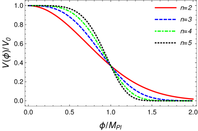
Figure 1: The form of the generalized exponential potential (7) for different values of $n$ and by choosing $\alpha=1$.

Let us now confirm that WI can indeed gracefully exit in the runaway part of the potential. WI ends when $\epsilon_{V}\approx 1+Q$, or $\epsilon_{WI}\approx 1$. Therefore, to end inflation, $\epsilon_{WI}$ should be an increasing function of number of $e$-foldings yielding a condition Das:2020lut

$$\frac{d\ln\epsilon_{V}}{dN}>\frac{Q}{1+Q}\frac{d\ln Q}{dN}.$$ (27)

For the runaway potential in Eq. (7) the slow-roll parameters become

$$\!\!\!\!\!\!\!\!\!\epsilon_{V} = \frac{\alpha^{2}n^{2}}{2}\left(\frac{\phi}{M_{\rm Pl}}\right)^{2n-2},$$ (28)

$$\!\!\!\!\!\!\!\!\!\eta_{V} = \alpha^{2}n^{2}\left(\frac{\phi}{M_{\rm Pl}}\right)^{2n-2}\!\!\!-\alpha n(n-1)\left(\frac{\phi}{M_{\rm Pl}}\right)^{n-2}.$$ (29)

The slow-roll parameter $\epsilon_{V}$ evolves with the number of $e$-foldings as

$$\frac{d\ln\epsilon_{V}}{dN}=\frac{4\epsilon_{V}-2\eta_{V}}{1+Q}=\frac{\alpha n(n-1)}{1+Q}\left(\frac{\phi}{M_{\rm Pl}}\right)^{n-2}.$$ (30)

This shows that $\epsilon_{V}$ is a constant and does not evolve when $n=1$, and it does evolve for $n>1$. We are interested in the part of the potential for which $\phi>\phi_{\rm inflection}$. We then get from Eq. (30) that

$$\left(\frac{\phi}{M_{\rm Pl}}\right)^{n}=\frac{d\ln\epsilon_{V}}{dN}\frac{1+Q}{\alpha n(n-1)}\left(\frac{\phi}{M_{\rm Pl}}\right)^{2}.$$ (31)

The left hand side of the above equation has to be greater than $(n-1)/n\alpha$ such that inflation takes place in the steep slope of the potential. Thus, in this range we get

$$\frac{d\ln\epsilon_{V}}{dN}>\frac{(n-1)^{2}}{1+Q}\left(\frac{\phi}{M_{\rm Pl}}\right)^{-2}.$$ (32)

As the right hand side of the above inequality is always positive, $\epsilon_{V}$ would always increase when inflation is taking place in the steep region of the slope. Thus, inflation is assured to end whenever $Q$ is constant or decreases with $e$-foldings. However, inflation can also end when $Q$ increases with $N$ but with a slower rate than the evolution of $\epsilon_{V}$ as shown in Eq. (27). This is, however, a more difficult condition to achieve in general.

With the form of the dissipative coefficient given in Eq. (25), the dissipation ratio $Q$ evolves as

$$\frac{d\ln Q}{dN}=\frac{10\epsilon_{V}-6\eta_{V}}{1+7Q}.$$ (33)

In the strong dissipative regime ($Q\gg 1$) the condition to end inflation given in Eq. (27) then becomes

$$9\epsilon_{V}>4\eta_{V},$$ (34)

which yields

$$\left(\frac{\phi}{M_{\rm Pl}}\right)^{n}>-\frac{8(n-1)}{n\alpha}.$$ (35)

As we are only interested in the region beyond the inflection point, this condition will always be satisfied in the region of our interest. Thus, inflation will always end in the steep potential region beyond the inflection point.

III.2 The perturbations

Now, let us consider the perturbations in this theory. The form of the scalar power spectrum in WI has already been discussed in Eq. (19) and Eq. (20). In this case, the form for the function $G(Q_{*})$, valid for the generalized exponential potential Eq. (7), is found to be given by (see also discussion concerning this point in the Appendix B).

$$G(Q_{*}) = \frac{1+6.12Q_{*}^{2.73}}{\left(1+6.96Q_{*}^{0.78}\right)^{0.72}}$$ (36)

$$+ \frac{0.01Q_{*}^{4.61}\left(1+4.82\times 10^{-6}Q_{*}^{3.12}\right)}{\left(1+6.83\times 10^{-13}Q_{*}^{4.12}\right)^{2}},$$

which is found to hold up to rather large values of $Q_{*}$ ($Q_{*}\sim 3\times 10^{3}$). This will be enough to cover the range of values of $Q$ to be considered in the next section.

Note that the scalar power spectrum used in Ref. Berghaus:2019whh was of the form (see, e.g., Eq. (12) in that reference),

$$\Delta_{\mathcal{R}}\approx\frac{\sqrt{3}}{4\pi^{\frac{3}{2}}}\frac{H^{3}T}{\dot{\phi}^{2}}\left(\frac{Q}{Q_{3}}\right)^{9}Q^{\frac{1}{2}},$$ (37)

where $Q_{3}\approx 7.3$. It can be easily shown that in the strong dissipative regime a more accurate form of the power spectrum given in Eq. (19), along with the relations given in Eq. (20) and Eq. (36), does not differ much from the above equation. As the above equation is presented in a much simpler form for the strong dissipative regime, we will derive the scalar spectral index analytically using the form of the power spectrum given in Eq. (37) for simplicity (while numerically we will use the full form of the function $G(Q)$ given in Eq. (36) to calculate the spectral index). We see that

$$n_{s}-1=3\frac{d\ln H}{dN}-2\frac{d\ln\dot{\phi}}{dN}+\frac{d\ln T}{dN}+\frac{19}{2}\frac{d\ln Q}{dN}.$$

To determine the quantities on the right hand side of the above equations, we will use the approximated background equations given in Eqs. (16), along with the approximated forms of $Q$ and $T$ valid for the form of the dissipation coefficient given by Eq. (25) (see also Ref. Berghaus:2019whh ),

$$Q^{7}\approx\tilde{C}_{Q}\frac{V^{\prime 6}}{V^{5}},\quad T^{7}\approx\tilde{C}_{T}\frac{V^{\prime 2}}{V^{1/2}},$$ (39)

which are valid in a strong dissipative regime. From these equations, we see that

$$\frac{d\ln H}{dN}\sim-\frac{\epsilon_{V}}{Q},\quad\frac{d\ln Q}{dN}\sim\frac{10\epsilon_{V}-6\eta_{V}}{7Q},$$

$$\frac{d\ln T}{dN}\sim\frac{\epsilon_{V}-2\eta_{V}}{7Q},\quad\frac{d\ln\dot{\phi}}{dN}\sim-\frac{3\epsilon_{V}+\eta_{V}}{7Q}.$$ (40)

Inserting all these in the expression of $n_{s}$, we get Berghaus:2019whh

$$n_{s}-1=\frac{3}{7Q}(27\epsilon_{V}-19\eta_{V}),$$ (41)

It is to note that, to obtain a red-tilt of the scalar spectrum one requires a potential yielding $\eta_{V}>\epsilon_{V}$, as has also been observed in Ref. Berghaus:2019whh . To be more precise, we need $19\eta_{V}>27\epsilon_{V}$, which yields a condition

$$\left(\frac{\phi}{M_{\rm Pl}}\right)^{n}>\frac{38(n-1)}{11n\alpha}.$$ (42)

This is a stronger bound on the field range than the one required for field ranges beyond the inflection point. Therefore, beyond the above range, inflation ends as well as we get the desired spectral index with appropriate choices of $\alpha$ for a given $n$. These findings are explicitly checked in our numerical examples considered in the next section.

IV Numerical analysis of the parameter ranges

We have numerically evolved the full background equations given in Eqs (10) for the cases $n=2$ to 5 and the findings are furnished in the Table 1. In principle, we can tune appropriately both $Q_{*}$ and the constant $\alpha$ of the potential, for a given value of $n$, such as to produce results consistent with the observable quantities for either smaller or larger values of $Q_{*}$ than the ones shown in Table 1. Our criteria for choosing the value of $Q_{*}$ was that it would be large enough such that all the swampland criteria could be met as also to have $n_{s}$ around the central value from the Planck analysis. The tensor-to-scalar ratio $r$ is naturally very much suppressed in the large $Q$ regime of WI, as already seen in other cases (see, e.g., Refs. Bastero-Gil:2019gao ; Kamali:2019xnt ). The second and third column containing the values of $n_{s}$ and $r$, respectively ensures that the models with different values of $n$ (and the chosen values of $\alpha$ accordingly) are in accordance with the observations. The fifth column shows the amount of field traversed, $\Delta\phi$, which turns out to be sub-Planckian for all the cases and it confirms that these examples obey the Swampland distance conjecture. The tenth and the eleventh column, which contain the values of the slow-roll parameters $\epsilon_{V}$ and $\eta_{V}$, respectively, which are much larger than unity, ensure that the Swampland de Sitter conjecture is maintained. The last column, which quotes the values of $V_{*}$, i.e., the scale of inflation, confirms that the TCC is obeyed as well. Hence, Table 1 confirms that the runaway potentials with $n>1$ not only remain in tune with observations but also obey all the three Swampland conjectures, making these models prime candidates as consistent effective field theory models in String Landscapes.

Model	$n_{s}$	$r$	$N_{*}$	$\Delta\phi/M_{\rm Pl}$	$C_{\Upsilon}$	$M/M_{\rm Pl}$	$T_{\rm end}$ (GeV)	$V_{0}$ (GeV)4	$\epsilon_{V_{*}}$	$\eta_{V_{*}}$	$V_{*}^{1/4}/M_{\rm Pl}$
$n=2$
$\alpha=9.6$	0.9648	$4.89\times 10^{-29}$	48.0	0.98	$6.04\times 10^{-11}$	$4.0\times 10^{-13}$	$1.52\times 10^{7}$	$3.07\times 10^{38}$	31.7	44.2	$1.52\times 10^{-11}$
$Q_{*}=850.96$
$n=3$
$\alpha=2.5$	0.9689	$1.44\times 10^{-28}$	48.2	0.97	$4.19\times 10^{-11}$	$4.0\times 10^{-13}$	$2.49\times 10^{7}$	$1.82\times 10^{39}$	25.9	37.2	$2.49\times 10^{-11}$
$Q_{*}=740.15$
$n=4$
$\alpha=0.45$	0.9655	$1.83\times 10^{-28}$	48.1	0.97	$3.86\times 10^{-11}$	$4.0\times 10^{-13}$	$2.86\times 10^{7}$	$3.59\times 10^{39}$	25.0	36.5	$2.85\times 10^{-11}$
$Q_{*}=719.68$
$n=5$
$\alpha=0.06$	0.9645	$2.37\times 10^{-28}$	48.2	0.97	$3.53\times 10^{-11}$	$4.0\times 10^{-13}$	$3.18\times 10^{7}$	$6.01\times 10^{39}$	24.1	35.6	$3.18\times 10^{-11}$
$Q_{*}=699.53$

Table 1: Numerical estimation of respective parameters and the relevant cosmological quantities obtained from them.

For completeness, we have also shown in Fig. 2 how the potential, kinetic and radiation energy densities evolve with the number of $e$-foldings for the $n=3$ case. The situation for the other models with $n=2,\,4$ and 5 are very much similar, so we do not show them explicitly here. It can be seen that inflation ends when the radiation energy density starts to dominate over the potential energy density, while the kinetic energy density remains small all along.

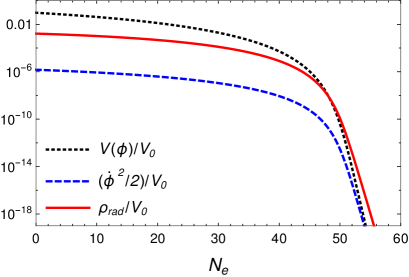
Figure 2: The evolution of the potential, kinetic and radiation energy densities for the model with $n=3$ given in Table 1.

As an additional point to be commented, and also related to the result shown in Fig. 2, is the number of efolds shown in the fourth column of Table 1. As noticed from Fig. 2, WI exists gracefully at around 48 $e-$foldings, when the energy scale of inflation is as low as $10^{-11}\,M_{\rm Pl}$. In WI we can precisely determine the number of e-folds of inflation $N_{*}$ between the moment the relevant scales with wavenumber $k_{*}$ leaving the Hubble radius and reentering around today. This is due to the fact that WI is not followed by a reheating phase and, thus, there is no uncertainty associated with the total number of $e$-folds which generally appears due to the uncertainty in the number of $e$-foldings of the reheating phase. By relating the comoving Hubble scale at $N_{*}$ when the mode with comoving wavenumber $k_{*}$ crossed the horizon, $a_{*}H_{*}=k_{*}$, with the one at present time, $a_{0}H_{0}$, we have that Liddle:2003as

$$\frac{k_{*}}{a_{0}H_{0}}=\frac{a_{*}}{a_{\rm end}}\frac{a_{\rm end}}{a_{\rm reh}}\frac{a_{\rm reh}}{a_{0}}\frac{H_{*}}{H_{0}},$$ (43)

where $a_{*}/a_{\rm end}=\exp(-N_{*})$ and we can use the fact that at the end of WI the universe smoothly transits to the radiation dominated regime with no intermediary reheating phase, hence, $a_{\rm end}/a_{\rm reh}=1$. This is particularly well satisfied for all the models exemplified in Table 1. Furthermore, as also seen in Fig. 2, inflation ends when $V(\phi)$ drops below $\rho_{R}$, while the kinetic energy density $\dot{\phi}^{2}/2$ remains always subdominant, even after inflation. Therefore, there is no kination period as is observed in general for these type of runaway exponential potentials. Finally, we can relate $a_{\rm end}\equiv a_{\rm reh}$ with $a_{0}$ in Eq. (43) by assuming that after WI there is no additional sources of entropy and use then the entropy conservation result,

$$g_{s}(T_{\rm end})T_{\rm end}^{3}a_{\rm end}^{3}=\left(2T_{0}^{3}+\frac{21}{4}T_{\nu,0}^{3}\right)a_{0}^{3},$$ (44)

where $T_{0}$ and $T_{\nu,0}=(4/11)^{1/3}T_{0}$ are, respectively, the today’s (CMB) photon and neutrino temperatures and we have explicitly used the respective number of degrees of freedom, while $g_{s}(T_{\rm end})$ is the effective number of degrees of freedom at the end of WI.

Putting the above relations together, Eq. (43), in WI, becomes

$$\frac{k_{*}}{a_{0}H_{0}}=e^{-N_{*}}\left[\frac{43}{11g_{s}(T_{\rm end})}\right]^{1/3}\frac{T_{0}}{T_{\rm end}}\frac{H_{*}}{H_{0}}.$$ (45)

Here, we take the convention that $a_{0}=1$. For the Hubble parameter today, we assume the Planck result, $H_{0}=67.66\,{\rm km}\,s^{-1}{\rm Mpc}^{-1}$ [from the Planck Collaboration Aghanim:2018eyx , TT,TE,EE-lowE+lensing+BAO 68$\%$ limits, $H_{0}=(67.66\pm 0.42)\,{\rm km}\,s^{-1}{\rm Mpc}^{-1}$]. Likewise, for the CMB temperature today we assume the value $T_{0}=2.725\,{\rm K}=2.349\times 10^{-13}\,{\rm GeV}$, while the for the pivot scale $k_{*}$ we take the Planck value $k_{*}=0.05/{\rm Mpc}$. For $g_{s}(T_{\rm end})$ we assumed the standard model value, $g_{s}(T_{\rm end})=106.75$, for definiteness (the results are very weakly dependent on $g_{s}$). Putting all these values in the above equation, $N_{*}$ turns out to be of order 48, consistent with the results seen in Table 1.

As a final remark about the observational predictions of the models studied here, concerns the level of non-Gaussianity that they produce. For WI in the large dissipative regime, as is the case for all models we have considered, it is predicted a non-Gaussianity coefficient of the warm shape (see, e.g., Ref. Bastero-Gil:2014raa for details) as large as $|f_{\rm NL}^{\rm warm}|\sim 5$ in the case of a dissipation coefficient $\Upsilon\propto T^{3}$. This is still within the range of the results obtained by the Planck 2018 team using the WI shape Akrami:2019izv , $f_{\rm NL}^{\rm warmS}=-48\pm 27$ (from SMICA+T+E, $68\%$ C.L.) and $f_{\rm NL}^{\rm warmS}=-39\pm 44$ (from SMICA+T, $68\%$ C.L.). But the expected result that we have for $f_{\rm NL}$, for all the cases here studied, is still in a magnitude that can be large enough to possibly be probed from, e.g., the future fourth generation CMB observatories Abazajian:2016yjj , or from future large scale structure surveys. Both of these are expected to bring down the present upper bounds on non-Gaussianities. Thus, non-Gaussianity can be one of the indicators differentiating WI in the strong dissipative regime from the weak dissipative one, through their distinct non-Gaussianity shapes and predictions for $f_{\rm NL}$ Bastero-Gil:2014raa .

V Conclusion

The proposed Swampland conjectures, namely the Swampland Distance conjecture, the de Sitter conjecture and the Transplanckian Censorship Conjecture, have severely constrained the construction of viable inflation models in any String Landscape. Thus, the swampland program strongly restricts the class of possible effective field theory models of inflation that are consistent with quantum gravity. It is thus worthwhile to look for constructions where the inflationary dynamics can be accommodated away from Swamplands. It has been pointed out previously that the WI scenario befits the Swampland Conjectures, especially the de Sitter one, much better than its counter part, the cold inflation paradigm. The de Sitter conjecture is also better suited with the runaway type of potentials (like, e.g., Eq. (7)) which do not have any critical points. In particular, it has already been demonstrated that the de Sitter conjecture also remains robust in WI Brandenberger:2020oav . Besides of this, it has been a challenge, even for WI, to satisfy the TCC, which in its original formulation Bedroya:2019tba , requires inflation to happen at sufficiently small scales. The difficulty is associated with the construction of WI models able to support strong enough dissipation and at the same time to be consistent with the observations Bastero-Gil:2019gao . Even models motivated by WI, like the ones studied in Ref. Berera:2020iyn , reflects well this difficulty. It is thus an important task finding appropriate inflation models that are able to satisfy all the swampland criteria. In the present paper, we have explicitly considered the validity of runaway type of potentials when embedding them in WI.

It was previously shown that the runaway potential with exponent $n=1$ can be embedded in a Randall-Sundrum braneworld inflation successfully where it can observe all the three Swampland conjectures Kamali:2019xnt . However, when such a potential is embedded in a standard general relativity context with WI, it yields too much red tilt in the scalar power spectrum to be in accordance with the observations Goswami:2019ehb . In this work we have examined the runaway potentials with exponents $n>1$ when embedded in WI models characterized by a cubic in the temperature dependence of the dissipation coefficient to show that (a) such models gracefully exists inflation when inflation takes place in the runaway part of the potential; (b) they can remain in tune with the current observations by yielding the correct scalar spectral index, and (c) they can also simultaneously satisfy all the three Swampland conjectures as a consequence of supporting a strong enough dissipative regime of WI. The combination of all these features make these type of models viable inflation models when constructed in the WI picture and which can be realized within String landscapes.

Appendix A The dissipation coefficient

Dissipative effects are expected to be experienced by systems, when displaced from their state of equilibrium and interacting with an environment. We can consider the case of a background scalar field $\phi$ initially displaced from its equilibrium state and interacting with other fields $X$. Given an interaction Lagrangian density like

$${\cal L}_{\rm int}(\phi,X)=-f(\phi)g(X).$$ (46)

A proper study of the evolution of the background field can be performed in the context of the in-in, or the closed-time path (CTP) functional formalism Calzetta:2008iqa . By integrating over the $X$ field, a nonlocal effective equation of motion for $\phi$ can be derived and the ensemble averaged effective equation of motion for $\phi$ can be generically expressed like Calzetta:2008iqa

$$\partial_{\mu}\frac{\partial{\cal L}_{\rm eff,r}[\phi]}{\partial(\partial_{\mu}\phi)}-\frac{\partial{\cal L}_{\rm eff,r}[\phi]}{\partial\phi}-i\frac{\partial f(\phi)}{\partial\phi}\int d^{4}x^{\prime}\theta(t-t^{\prime})\left[f(\phi(x^{\prime}))-f(\phi(x))\right]\langle[g(X(x)),g(X(x^{\prime}))]\rangle=0,$$ (47)

where ${\cal L}_{\rm eff,r}[\phi]$ is the renormalized effective Lagrangian density for $\phi$ and $\langle\cdots\rangle$ are ensemble averages with respect to an equilibrium (quantum or thermal) state. Equation (47) form the basis of the many earlier works Gleiser:1993ea ; Berera:1998gx ; Berera:2001gs ; Berera:2004kc ; Berera:2007qm (for a review, see also Ref. Berera:2008ar ) that evolved to warm inflation model realizations. The non-local term in Eq. (47) represents a transfer of energy from the $\phi$ field into radiation. The nonlocal term in Eq. (47) can be localized and expressed in a form of a proper dissipation term when there is a separation of timescales between the system and environment, e.g., given a response timescale $\tau$ related to the plasma interactions and $\phi$ is slowly varying on the response timescale $\tau$, $\dot{\phi}/\phi\ll\tau^{-1}$, which is typically referred to as the adiabatic approximation, then we can write Berera:2007qm

$$-i\frac{\partial f(\phi)}{\partial\phi}\int d^{4}x^{\prime}\theta(t-t^{\prime})\left[f(\phi(x^{\prime}))-f(\phi(x))\right]\langle[g(X(x)),g(X(x^{\prime}))]\rangle\approx\Upsilon\dot{\phi},$$ (48)

where $\Upsilon$ is the dissipation coefficient defined as

$$\Upsilon=\int d^{4}x^{\prime}\Sigma_{R}(x,x^{\prime})(t^{\prime}-t)=-\lim_{\omega\to 0}\frac{{\rm Im}\Sigma_{R}({\bf k}={\bf 0},\omega)}{\omega},$$ (49)

where $\Sigma_{R}(\omega)$ is the Fourier-transform of the retarded correlation function,

$$\Sigma_{R}(x,x^{\prime})=-i\left[\frac{\partial f(\phi)}{\partial\phi}\right]^{2}\theta(t-t^{\prime})\langle[g(X(x)),g(X(x^{\prime}))]\rangle.$$ (50)

Many examples of dissipation coefficients were for example derived in Ref. BasteroGil:2010pb . As discussed in the Introduction, in this work we are particularly interested in models leading to a dissipation coefficient that scales with the cubic power in the temperature, $\Upsilon\propto T^{3}$. Let us briefly review viable interaction schemes leading to such a dissipation coefficient.

A.1 Dissipation through a catalyst heavy field

One of the first working field theory model for WI has been constructed in the case of the inflaton field dissipating to light radiation fields intermediate by a heavy catalyst field. The implementation is based on a supersymmetric model with chiral superfields $\Phi$, $X$ and $Y_{i}$, $i=1,\ldots,N_{Y}$, described by the superpotential Berera:2008ar ,

$$W={g\over 2}\Phi X^{2}+{h_{i}\over 2}XY_{i}^{2}+f(\Phi)~{},$$ (51)

where a sum over the index $i$ is implicit. The scalar component of the superfield $\Phi$ describes the inflaton field, with an expectation value $\phi=\phi/\sqrt{2}$ and $f(\Phi)$ describes the self-interactions in the inflaton sector. The $X$ fields are assumed to be heavy fields with respect to the radiation bath temperature produced by the light fields $Y$, i.e., $m_{X}\gg T$ and $m_{Y}\ll T$. Under these circumstances, the dissipation coefficient in the inflaton’s equation of motion can be shown to be given by BasteroGil:2010pb ; BasteroGil:2012cm

$$\Upsilon\simeq C_{\Upsilon}\frac{T^{3}}{\phi^{2}},\;\;\;C_{\Upsilon}\simeq\frac{\alpha_{h}}{4}N_{X}N_{Y},$$ (52)

where $\alpha_{h}=h^{2}N_{Y}/(4\pi)$, $N_{X}$ is the number of fields in the $X$ heavy sector and it was assumed $h=h_{i}$ for all the light fields for simplicity. despite the dependence on the inflaton field in Eq. (52), the results obtained for this model do not differ much from the ones we have obtained in Sec. IV. It can likewise support strong dissipation and satisfy all the swampland criteria and with an observationally consistent $n_{s}$. However, for $Q\sim{\cal O}(700)$ as in Table 1, we have instead that $C_{\Upsilon}\sim 10^{14}$, which, from Eq. (52) and assuming $h\sim 1$, it implies the need of a huge number of heavy and/or light fields, $N_{X}N_{Y}\sim 5\times 10^{15}$. Such a large number might be a technical challenge associated with this model, from both the perturbativity and the unitarity point of view, associated with this model for the present analysis (see, however, Ref. BasteroGil:2011mr for a possible scenario where these issues can be overcame and that uses brane constructions, or also the proposal in Ref. Matsuda:2012kc where large field multiplicities can be allowed due to a Kaluza-Klein tower in extra-dimensional scenarios).

A.2 Dissipation in the Minimal Warm Inflation model

The Minimal Warm Inflation (MWI) model was proposed by the authors in Ref. Berghaus:2019whh . In the MWI model the inflaton field has axion-like couplings to non-Abelian gauge fields which yields a viable model of the thermal bath that can exist during WI. The inflaton field is coupled to a Yang-Mills field $A_{\mu}^{a}$ in an axion-like form,

$${\cal L}_{\rm int}=\frac{\alpha_{g}}{8\pi}\frac{\phi}{f}\tilde{F}^{a\,\mu\nu}F^{a}_{\mu\nu},$$ (53)

where the dual gauge field strength $\tilde{F}^{a\,\mu\nu}=\frac{1}{2}\epsilon^{\mu\nu\alpha\beta}F^{a}_{\alpha\beta}$, $F_{\mu\nu}^{a}=\partial_{\mu}A_{\nu}^{a}-\partial_{\nu}A_{\mu}^{a}+gC^{abc}A_{\mu}^{b}A_{\nu}^{c}$, with $g$ the Yang-Mills coupling and $C^{abc}$ is the structure constant of the non-Abelian group. In Eq. (53) one also has that $\alpha_{g}\equiv g^{2}/(4\pi)$ and $f$ is an scale analogous to the axion decay constant. The corresponding dissipative coefficient that the interaction produces has been shown to be related to the Chern-Simons diffusion rate and given by Moore:2010jd ; Laine:2016hma

$$\Upsilon=C_{\Upsilon}\frac{T^{3}}{f^{2}},\;\;\;C_{\Upsilon}=\kappa(\alpha_{g},N_{c},N_{f})\alpha_{g}^{5},$$ (54)

where $N_{c}$ is the dimension of the gauge group, $N_{f}$ is the representation of the fermions if any, and $\kappa$ is a dimensional quantity depending on $N_{c}$, $N_{f}$ and $\alpha_{g}$.

One of the advantages of this model is that the shift symmetry satisfied by the inflaton naturally protects it from large thermal corrections that might undermine the slow-roll conditions during inflation.

It is useful to estimate the scale $f$ appearing in Eq. (54) from our numerical results given in Table 1. Using that $\kappa\sim 100$ and $g\sim 0.1$, then from the values for $C_{\Upsilon}$ and $M$ given in Table 1, we find that for all models analyzed $f\sim 5\times 10^{4}$ GeV. It is clear that in the present context we cannot associate $\phi$ with the quantum cromodynamics (QCD) axion, since $f$ is much below the astrophysical lower bound $f\gtrsim 10^{9}$ GeV set in for the QCD axion decay constant Sikivie:2020zpn .

A.3 Dissipation through derivative couplings with the inflaton field

A third option to produce dissipation coefficients behaving like $\Upsilon\propto T^{3}$ is motivated from the previous example. We consider the case where the inflaton has a moduli-like (or dilaton-like) derivative coupling with other radiation fields, which can be for example other scalar fields and with an interaction Lagrangian density given by

$${\cal L}_{\rm int}=g^{2}\frac{\phi}{2M}(\partial_{\mu}\chi)^{2}.$$ (55)

The scalar field $\chi$ is supposed to remain in thermal equilibrium through either its self-coupling or to couplings to other radiation fields (e.g., additional gauge or other light fields that could be added to the model). It has been realized in Ref. Bodeker:2006ij that the dissipation coefficient in this model can be precisely related to the bulk viscosity calculation for a scalar field Jeon:1994if , leading then to the result for the dissipation coefficient given by

$$\Upsilon\simeq 4.5g^{4}\frac{\ln^{2}(\xi\lambda)}{\lambda}\frac{T^{3}}{M^{2}},$$ (56)

where $\xi$ is a numerical constant, $\xi=\exp[15\zeta(3)/\pi^{2}]\simeq 0.064736$, and $\lambda$ is the quartic self-coupling for the $\chi$ field, $-\lambda\chi^{4}/4!$. It is interesting to observe that this connection of the dissipation coefficient in WI at high temperature with a viscosity coefficient was already noticed in Ref. Berera:1998gx .

An additional interaction that now makes the connection with the bulk viscosity calculation in a pure gauge theory is by coupling the moduli field now to pure Yang-Mills gauge fields through a coupling like (note that this is different from the interaction term in Eq. (53)

$${\cal L}_{\rm int}=-g^{2}\frac{\phi}{2M}F^{a\,\mu\nu}F^{a}_{\mu\nu},$$ (57)

which gives for the dissipation coefficient the result Laine:2010cq ; Laine:2016hma

$$\Upsilon\simeq\frac{(12\pi\alpha_{g})^{2}}{\ln(1/\alpha_{g})}\frac{T^{3}}{M^{2}},$$ (58)

where, as before, $\alpha_{g}\equiv g^{2}/(4\pi)$.

It remains, as possible future work, to see how the above moduli-like interactions can be implemented in an explicit quantum field theory model building construction for WI.

Appendix B Perturbations in warm inflation

We review here the first-order perturbation equations for WI, consisting of the inflaton perturbations $\delta\phi$, the radiation energy density perturbation $\delta\rho_{r}$ and the radiation momentum perturbation $\Psi_{r}$. The notation that we follow is the one given in Refs. Hwang:1991aj ; Hwang:2001fb .

The perturbed FLRW metric is given by

$$ds^{2} = -(1+2\alpha)dt^{2}-2a\partial_{i}\beta dx^{i}dt$$ (59)

$$+ a^{2}[\delta_{ij}(1+2\varphi)+2\partial_{i}\partial_{j}\gamma]dx^{i}dx^{j},$$

where $\alpha$, $\beta$, $\gamma$ and $\varphi$ are the spacetime-dependent perturbed-order variables. These metric perturbation functions are related to the complete set of equations (when Fourier transforming to space-momentum) Hwang:1991aj ; Hwang:2001fb

$$\chi=a(\beta+a\dot{\gamma})\,,$$ (60)

$$\kappa=3(H\alpha-\dot{\varphi})+\frac{k^{2}}{a^{2}}\chi\,,$$ (61)

$$-\frac{k^{2}}{a^{2}}\varphi+H\kappa=-\frac{1}{2M_{\rm Pl}^{2}}\delta\rho\,,$$ (62)

$$\kappa-\frac{k^{2}}{a^{2}}\chi=-\frac{3}{2M_{\rm Pl}^{2}}\Psi\,,$$ (63)

$$\dot{\chi}+H\chi-\alpha-\varphi=0\,,$$ (64)

$$\dot{\kappa}+2H\kappa+\left(3\dot{H}-\frac{k^{2}}{a^{2}}\right)\alpha=\frac{1}{2M_{\rm Pl}^{2}}\left(\delta\rho+3\delta p\right)\,,$$ (65)

where $\delta\rho$, $\delta p$ and $\Psi$ are, respectively, the total density, pressure and momentum perturbations. In our two-fluid system (inflaton plus radiation), they are given in terms of the inflaton field and radiation perturbations, e.g.,

$$\delta\rho=\delta\rho_{\phi}+\delta\rho_{r}\,,$$ (66)

$$\delta p=\delta p_{\phi}+\delta p_{r}\,,$$ (67)

$$\Psi=\Psi_{\phi}+\Psi_{r}\,,$$ (68)

with $\delta\rho_{\phi}=\dot{\phi}\delta\dot{\phi}-\dot{\phi}^{2}\alpha+V_{,\phi}\delta\phi$, $\delta p_{\phi}=\dot{\phi}\delta\dot{\phi}-\dot{\phi}^{2}\alpha-V_{,\phi}\delta\phi$, $\delta p_{r}=\omega_{r}\delta\rho_{r}$ and $\Psi_{\phi}=-\dot{\phi}\delta\phi$ (with “dot” always denoting derivative with respect to the cosmic time).

The evolution equations for the field and radiation perturbation quantities follow from the conservation of the energy-momentum tensor. The complete equations have been given in Ref. BasteroGil:2011xd , which we indicate the interested reader for more details. Working in momentum space, defining the Fourier transform with respect to the comoving coordinates, the equation of motion for the radiation and momentum fluctuations with comoving wavenumber $k$ are given by

$$\delta\dot{\rho_{r}}+4H\delta\rho_{r}=(1+\omega_{r})\rho_{r}\left(\kappa-3H\alpha\right)$$

$$+\frac{k^{2}}{a^{2}}\Psi_{r}+\delta Q_{r}+Q_{r}\alpha\,,$$ (69)

$$\dot{\Psi}_{r}+3H\Psi_{r}+\omega_{r}\delta\rho_{r}+\delta\Pi=-(1+\omega_{r})\rho_{r}\alpha+J_{r},$$

(70)

where

$$Q_{r}=\Upsilon\dot{\phi}^{2},$$ (71)

$$\delta Q_{r}=\delta\Upsilon\dot{\phi}^{2}+2\Upsilon\dot{\phi}\delta\dot{\phi}-2\alpha\Upsilon\dot{\phi}^{2}\,,$$ (72)

$$J_{r}=-\Upsilon\dot{\phi}\delta\phi.$$ (73)

In addition to Eqs. (69) and (70), there is also the evolution equation for the field fluctuations $\delta\phi$, which is described by a stochastic evolution determined by a Langevin-like equation Graham:2009bf :

$$\delta\ddot{\phi}+3H\delta\dot{\phi}+\left(\frac{k^{2}}{a^{2}}+V_{,\phi\phi}\right)\delta\phi=\xi_{q}+\xi_{T}-\delta\Upsilon\dot{\phi}$$

$$+\dot{\phi}(\kappa+\dot{\alpha})+(2\ddot{\phi}+3H\dot{\phi})\alpha-\Upsilon(\delta\dot{\phi}-\alpha\dot{\phi})\,,$$ (74)

where $\xi_{q,T}\equiv\xi_{q,T}({\bf k},t)$ are stochastic Gaussian sources related to quantum and thermal fluctuations with appropriate amplitudes (for details and for their complete definitions, see Ref. Ramos:2013nsa ).

To complete the specification of the fluctuation equations, we need $\delta\Upsilon$, the fluctuation of the dissipation coefficient. For a general temperature $T$ and field $\phi$ dependent dissipative coefficient, given by Eq. (23), we have that

$$\delta\Upsilon=\Upsilon\left[p\frac{\delta T}{T}+c\frac{\delta\phi}{\phi}\right].$$ (75)

Although dissipation implies departures from thermal equilibrium in the radiation fluid, the system has to be close-to-equilibrium for the calculation of the dissipative coefficient to hold, therefore we assume $p_{r}\simeq\rho_{r}/3$ and, hence, $\omega_{r}=1/3$. Then, with $\rho_{r}\propto T^{4}$, we have that $\delta T/T\simeq\delta\rho_{r}/(4\rho_{r})$ and $\delta Q_{r}$ in Eq. (72) can be expressed as

$$\delta Q_{r}=3HQ\dot{\phi}^{2}\left(\frac{p\delta\rho_{r}}{4\rho_{r}}+\frac{c\delta\phi}{\phi}\right)+6HQ\dot{\phi}\delta\dot{\phi}-6HQ\dot{\phi}^{2}\alpha\,.$$ (76)

From the above relations, the complete system of first-order perturbation equations for WI become

$$\delta\ddot{\phi} = -3H\left(1+Q\right)\delta\dot{\phi}-\left(\frac{k^{2}}{a^{2}}+V_{,\phi\phi}+\frac{3cHQ\dot{\phi}}{\phi}\right)\delta\phi$$

$$+ \xi_{q}+\xi_{T}-\frac{pH}{\dot{\phi}}\delta\rho_{r}+\dot{\phi}(\kappa+\dot{\alpha})+[2\ddot{\phi}+3H(1+Q)\dot{\phi}]\alpha,$$

$$\delta\dot{\rho_{r}} = -H\left(4-\frac{3pQ\dot{\phi}^{2}}{4\rho_{r}}\right)\delta\rho_{r}+\frac{k^{2}}{a^{2}}\Psi_{r}+6HQ\dot{\phi}\delta\dot{\phi}$$

$$+\frac{3cHQ\dot{\phi^{2}}}{\phi}\delta\phi+\frac{4\rho_{r}}{3}\kappa-3H\left(Q\dot{\phi}^{2}+\frac{4\rho_{r}}{3}\right)\alpha,$$

$$\dot{\Psi}_{r} = -3H\Psi_{r}-3HQ\dot{\phi}\delta\phi-\frac{1}{3}\delta\rho_{r}-4\rho_{r}\frac{\alpha}{3}.$$ (79)

Equations (LABEL:deltaddotphi), (LABEL:deltadotrhor) and (79), together with the metric perturbations Eqs. (60) - (65), form a complete set of equations in a “gauge-ready” form. From this point on we can either choose to work in terms of gauge-invariant quantities Kodama:1985bj ; Hwang:1991aj , or equivalently just choose an appropriate gauge directly. Even though any appropriate gauge can be chosen, a convenient one showing good numerical stability when numerically integrating the full set of differential equations is the Newtonian slicing (or zero shear) gauge $\chi=0$. In the $\chi=0$ gauge, the relevant metric equations become

$$\kappa=\frac{3}{2M_{\rm Pl}^{2}}(\dot{\phi}\delta\phi-\Psi_{r})\,,$$ (80)

$$\alpha=-\varphi\,,$$ (81)

$$\dot{\varphi}=-H\varphi-\frac{1}{3}\kappa\,.$$ (82)

Finally, the power spectrum is determined from the comoving curvature perturbation ${\cal R}$, defined as

$$\Delta_{\cal R}(k)=\frac{k^{3}}{2\pi^{2}}\langle|{\cal R}|^{2}\rangle\,,$$ (83)

where “$\langle\cdots\rangle$” means average over different realizations of the noise terms in Eq. (LABEL:deltaddotphi) (see, for instance Refs. Graham:2009bf ; BasteroGil:2011xd ; Bastero-Gil:2014jsa for details of the numerical procedure). Finally, the comoving curvature perturbation ${\cal R}$ is composed of contributions not only from the metric perturbations and the inflaton momentum perturbations, but also from the radiation momentum perturbations,

$${\cal R}=\sum_{i=\phi,r}\frac{\rho_{i}+\bar{p}_{i}}{\rho+\bar{p}}{\cal R}_{i}\;,$$ (84)

$${\cal R}_{i}=-\varphi-\frac{H}{\rho_{i}+\bar{p}_{i}}\Psi_{i}\,,$$ (85)

with $\bar{p}=p_{\phi}+p_{r}$, $\bar{p}_{\phi}\equiv p_{\phi}$ and $\bar{p}_{r}=p_{r}$.

Note that in the literature there are different forms for which the resulting curvature perturbations are presented. For instance, by neglecting the explicit coupling between the inflaton and radiation perturbations, e.g., by setting the temperature power of the dissipation coefficient to zero, $p=0$, and dropping the metric perturbations (which are first-order in the slow-roll coefficients), Eq. (LABEL:deltaddotphi) can be explicitly solved Ramos:2013nsa , leading to the result, computed at Hubble radius crossing $k=aH$,

$$\Delta_{\cal R} = \frac{H^{3}T}{4\pi^{2}\dot{\phi}^{2}}\left[\frac{3Q}{2\sqrt{\pi}}2^{2\alpha}\frac{\Gamma\left(\alpha\right)^{2}\Gamma\left(\nu-1\right)\Gamma\left(\alpha-\nu+3/2\right)}{\Gamma\left(\nu-\frac{1}{2}\right)\Gamma\left(\alpha+\nu-1/2\right)}\right.$$ (86)

$$+ \left.\frac{H}{T}\coth\left(\frac{H}{2T}\right)\right],$$

where $\nu=3(1+Q)/2$, $\alpha=\sqrt{\nu^{2}+3\beta Q/(1+Q)-3\eta_{V}}$, $\beta=M_{\rm Pl}^{2}\Upsilon_{,\phi}V_{,\phi}/(\Upsilon V)$ and $\Gamma(x)$ is the Gamma-function. By dropping slow-roll coefficients, $\alpha\approx\nu$ and Eq. (86) can be very well approximated by the result

$$\!\!\!\!\!\!\!\!\!\!\!\!\!\Delta_{\cal R} \simeq \frac{H^{4}}{4\pi^{2}\dot{\phi}^{2}}\left[1+2n_{BE}(H/T)+\frac{2\sqrt{3}\pi Q}{\sqrt{3+4\pi Q}}{T\over H}\right],$$ (87)

where $n_{BE}$ is the Bose-Einstein distribution. In general we can also replace $n_{BE}$ by $n_{*}$, representing the statistical distribution state of the inflaton at Hubble radius crossing, which might not be necessarily that of thermal equilibrium. The form given by Eq. (87) is typically the result used in most of the recent literature in WI. When including the coupling between the inflaton and radiation perturbations shown in Eqs. (LABEL:deltaddotphi), (LABEL:deltadotrhor) and (79), these equations can only be solved numerically. The result is a correction to e.g. Eq. (87) which can be expressed in the form of a function $G(Q)$ of the dissipation coefficient and determined by a proper fitting of the numerical result for the curvature perturbation. In particular, for the cubic in the temperature dissipation coefficient studied in this work, we obtain Eq. (36). Note that there are varied ways in how the perturbation equations are solved, which lead to differences on how this function $G(Q)$ is presented in the literature. For instance, in the Ref. Graham:2009bf , where this effect of the coupling between inflaton and radiation perturbations in WI was first studied, an approximation to $G(Q)$ was given by neglecting both metric perturbations and other terms proportional to slow-roll coefficients in the perturbation equations and only the leading order dependence on $G(Q)$ through a simplified fitting was presented. Simpler fittings were also presented in Ref. BasteroGil:2011xd .

References

- (1) U. H. Danielsson and T. Van Riet, “What if string theory has no de Sitter vacua?,” Int. J. Mod. Phys. D 27, no.12, 1830007 (2018) doi:10.1142/S0218271818300070 [arXiv:1804.01120 [hep-th]].
- (2) S. Kachru, R. Kallosh, A. D. Linde and S. P. Trivedi, “De Sitter vacua in string theory,” Phys. Rev. D 68, 046005 (2003) doi:10.1103/PhysRevD.68.046005 [arXiv:hep-th/0301240 [hep-th]].
- (3) S. Sethi, “Supersymmetry Breaking by Fluxes,” JHEP 10, 022 (2018) doi:10.1007/JHEP10(2018)022 [arXiv:1709.03554 [hep-th]].
- (4) M. Dine, J. A. P. Law-Smith, S. Sun, D. Wood and Y. Yu, “Obstacles to Constructing de Sitter Space in String Theory,” [arXiv:2008.12399 [hep-th]].
- (5) G. Obied, H. Ooguri, L. Spodyneiko and C. Vafa, “De Sitter Space and the Swampland,” [arXiv:1806.08362 [hep-th]].
- (6) S. K. Garg and C. Krishnan, “Bounds on Slow Roll and the de Sitter Swampland,” JHEP 11, 075 (2019) doi:10.1007/JHEP11(2019)075 [arXiv:1807.05193 [hep-th]].
- (7) H. Ooguri, E. Palti, G. Shiu and C. Vafa, “Distance and de Sitter Conjectures on the Swampland,” Phys. Lett. B 788, 180-184 (2019) doi:10.1016/j.physletb.2018.11.018 [arXiv:1810.05506 [hep-th]].
- (8) P. Agrawal, G. Obied, P. J. Steinhardt and C. Vafa, “On the Cosmological Implications of the String Swampland,” Phys. Lett. B 784, 271-276 (2018) doi:10.1016/j.physletb.2018.07.040 [arXiv:1806.09718 [hep-th]].
- (9) P. Agrawal and G. Obied, “Dark Energy and the Refined de Sitter Conjecture,” JHEP 06, 103 (2019) doi:10.1007/JHEP06(2019)103 [arXiv:1811.00554 [hep-ph]].
- (10) H. Ooguri and C. Vafa, “On the Geometry of the String Landscape and the Swampland,” Nucl. Phys. B 766, 21-33 (2007) doi:10.1016/j.nuclphysb.2006.10.033 [arXiv:hep-th/0605264 [hep-th]].
- (11) A. Bedroya and C. Vafa, “Trans-Planckian Censorship and the Swampland,” [arXiv:1909.11063 [hep-th]].
- (12) A. Bedroya, R. Brandenberger, M. Loverde and C. Vafa, “Trans-Planckian Censorship and Inflationary Cosmology,” Phys. Rev. D 101, no.10, 103502 (2020) doi:10.1103/PhysRevD.101.103502 [arXiv:1909.11106 [hep-th]].
- (13) W. H. Kinney, S. Vagnozzi and L. Visinelli, “The zoo plot meets the swampland: mutual (in)consistency of single-field inflation, string conjectures, and cosmological data,” Class. Quant. Grav. 36, no.11, 117001 (2019) doi:10.1088/1361-6382/ab1d87 [arXiv:1808.06424 [astro-ph.CO]].
- (14) L. Aalsma and G. Shiu, “Chaos and complementarity in de Sitter space,” JHEP 05, 152 (2020) doi:10.1007/JHEP05(2020)152 [arXiv:2002.01326 [hep-th]].
- (15) S. Mizuno, S. Mukohyama, S. Pi and Y. L. Zhang, Phys. Rev. D 102, no.2, 021301 (2020) doi:10.1103/PhysRevD.102.021301 [arXiv:1910.02979 [astro-ph.CO]].
- (16) V. Kamali and R. Brandenberger, “Relaxing the TCC Bound on Inflationary Cosmology?,” Eur. Phys. J. C 80, no.4, 339 (2020) doi:10.1140/epjc/s10052-020-7908-8 [arXiv:2001.00040 [hep-th]].
- (17) A. Berera, S. Brahma and J. R. Calderón, “Role of trans-Planckian modes in cosmology,” [arXiv:2003.07184 [hep-th]].
- (18) S. Das, “Distance, de Sitter and Trans-Planckian Censorship conjectures: the status quo of Warm Inflation,” Phys. Dark Univ. 27, 100432 (2020) doi:10.1016/j.dark.2019.100432 [arXiv:1910.02147 [hep-th]].
- (19) A. Kehagias and A. Riotto, “A note on Inflation and the Swampland,” Fortsch. Phys. 66, no.10, 1800052 (2018) doi:10.1002/prop.201800052 [arXiv:1807.05445 [hep-th]].
- (20) S. Das, “Note on single-field inflation and the swampland criteria,” Phys. Rev. D 99, no.8, 083510 (2019) doi:10.1103/PhysRevD.99.083510 [arXiv:1809.03962 [hep-th]].
- (21) M. Motaharfar, V. Kamali and R. O. Ramos, “Warm inflation as a way out of the swampland,” Phys. Rev. D 99, no.6, 063513 (2019) doi:10.1103/PhysRevD.99.063513 [arXiv:1810.02816 [astro-ph.CO]].
- (22) S. Das, “Warm Inflation in the light of Swampland Criteria,” Phys. Rev. D 99, no.6, 063514 (2019) doi:10.1103/PhysRevD.99.063514 [arXiv:1810.05038 [hep-th]].
- (23) A. Mohammadi, T. Golanbari, H. Sheikhahmadi, K. Sayar, L. Akhtari, M. A. Rasheed and K. Saaidi, “Warm Tachyon Inflation and Swampland Criteria,” doi:10.1088/1674-1137/44/9/095101 [arXiv:2001.10042 [gr-qc]].
- (24) A. Berera, “Warm inflation,” Phys. Rev. Lett. 75, 3218-3221 (1995) doi:10.1103/PhysRevLett.75.3218 [arXiv:astro-ph/9509049 [astro-ph]].
- (25) R. Brandenberger, V. Kamali and R. O. Ramos, “Strengthening the de Sitter swampland conjecture in warm inflation,” [arXiv:2002.04925 [hep-th]].
- (26) A. Berera, I. G. Moss and R. O. Ramos, “Warm Inflation and its Microphysical Basis,” Rept. Prog. Phys. 72, 026901 (2009) doi:10.1088/0034-4885/72/2/026901 [arXiv:0808.1855 [hep-ph]].
- (27) M. Bastero-Gil and A. Berera, “Warm inflation model building,” Int. J. Mod. Phys. A 24, 2207-2240 (2009) doi:10.1142/S0217751X09044206 [arXiv:0902.0521 [hep-ph]].
- (28) A. Berera and J. R. Calderón, “Trans-Planckian censorship and other swampland bothers addressed in warm inflation,” Phys. Rev. D 100, no.12, 123530 (2019) doi:10.1103/PhysRevD.100.123530 [arXiv:1910.10516 [hep-ph]].
- (29) V. Kamali, M. Motaharfar and R. O. Ramos, “Warm brane inflation with an exponential potential: a consistent realization away from the swampland,” Phys. Rev. D 101, no.2, 023535 (2020) doi:10.1103/PhysRevD.101.023535 [arXiv:1910.06796 [gr-qc]].
- (30) A. R. Liddle, “Power Law Inflation With Exponential Potentials,” Phys. Lett. B 220, 502-508 (1989) doi:10.1016/0370-2693(89)90776-4
- (31) S. Das and R. O. Ramos, “On the graceful exit problem in warm inflation,” [arXiv:2005.01122 [gr-qc]].
- (32) S. Das, G. Goswami and C. Krishnan, “Swampland, Axions and Minimal Warm Inflation,” Phys. Rev. D 101, 10 (2020) doi:10.1103/PhysRevD.101.103529 [arXiv:1911.00323 [hep-th]].
- (33) K. V. Berghaus, P. W. Graham and D. E. Kaplan, “Minimal Warm Inflation,” JCAP 03, 034 (2020) doi:10.1088/1475-7516/2020/03/034 [arXiv:1910.07525 [hep-ph]].
- (34) C. Q. Geng, M. W. Hossain, R. Myrzakulov, M. Sami and E. N. Saridakis, “Quintessential inflation with canonical and noncanonical scalar fields and Planck 2015 results,” Phys. Rev. D 92, no.2, 023522 (2015) doi:10.1103/PhysRevD.92.023522 [arXiv:1502.03597 [gr-qc]].
- (35) C. Q. Geng, C. C. Lee, M. Sami, E. N. Saridakis and A. A. Starobinsky, “Observational constraints on successful model of quintessential Inflation,” JCAP 06, 011 (2017) doi:10.1088/1475-7516/2017/06/011 [arXiv:1705.01329 [gr-qc]].
- (36) S. Ahmad, R. Myrzakulov and M. Sami, “Relic gravitational waves from Quintessential Inflation,” Phys. Rev. D 96, no.6, 063515 (2017) doi:10.1103/PhysRevD.96.063515 [arXiv:1705.02133 [gr-qc]].
- (37) G. B. F. Lima and R. O. Ramos, “Unified early and late Universe cosmology through dissipative effects in steep quintessential inflation potential models,” Phys. Rev. D 100, no.12, 123529 (2019) doi:10.1103/PhysRevD.100.123529 [arXiv:1910.05185 [astro-ph.CO]].
- (38) M. Bastero-Gil, A. Berera, R. O. Ramos and J. G. Rosa, “Towards a reliable effective field theory of inflation,” [arXiv:1907.13410 [hep-ph]].
- (39) D. H. Lyth and A. R. Liddle, “The primordial density perturbation: Cosmology, inflation and the origin of structure,” (Cambridge University Press, Cambridge, 2009).
- (40) R. O. Ramos and L. A. da Silva, “Power spectrum for inflation models with quantum and thermal noises,” JCAP 03, 032 (2013) doi:10.1088/1475-7516/2013/03/032 [arXiv:1302.3544 [astro-ph.CO]].
- (41) M. Benetti and R. O. Ramos, “Warm inflation dissipative effects: predictions and constraints from the Planck data,” Phys. Rev. D 95, no.2, 023517 (2017) doi:10.1103/PhysRevD.95.023517 [arXiv:1610.08758 [astro-ph.CO]].
- (42) C. Graham and I. G. Moss, “Density fluctuations from warm inflation,” JCAP 07, 013 (2009) doi:10.1088/1475-7516/2009/07/013 [arXiv:0905.3500 [astro-ph.CO]].
- (43) M. Bastero-Gil, A. Berera and R. O. Ramos, “Shear viscous effects on the primordial power spectrum from warm inflation,” JCAP 07, 030 (2011) doi:10.1088/1475-7516/2011/07/030 [arXiv:1106.0701 [astro-ph.CO]].
- (44) M. Bastero-Gil, A. Berera, I. G. Moss and R. O. Ramos, “Cosmological fluctuations of a random field and radiation fluid,” JCAP 05, 004 (2014) doi:10.1088/1475-7516/2014/05/004 [arXiv:1401.1149 [astro-ph.CO]].
- (45) Y. Akrami et al. [Planck], “Planck 2018 results. X. Constraints on inflation,” [arXiv:1807.06211 [astro-ph.CO]].
- (46) N. Aghanim et al. [Planck], “Planck 2018 results. VI. Cosmological parameters,” [arXiv:1807.06209 [astro-ph.CO]].
- (47) Y. Zhang, “Warm Inflation With A General Form Of The Dissipative Coefficient,” JCAP 03, 023 (2009) doi:10.1088/1475-7516/2009/03/023 [arXiv:0903.0685 [hep-ph]].
- (48) L. Visinelli, “Observational Constraints on Monomial Warm Inflation,” JCAP 07, 054 (2016) doi:10.1088/1475-7516/2016/07/054 [arXiv:1605.06449 [astro-ph.CO]].
- (49) I. G. Moss and C. Xiong, “On the consistency of warm inflation,” JCAP 11, 023 (2008) doi:10.1088/1475-7516/2008/11/023 [arXiv:0808.0261 [astro-ph]].
- (50) S. del Campo, R. Herrera, D. Pavón and J. R. Villanueva, “On the consistency of warm inflation in the presence of viscosity,” JCAP 08, 002 (2010) doi:10.1088/1475-7516/2010/08/002 [arXiv:1007.0103 [astro-ph.CO]].
- (51) M. Bastero-Gil, A. Berera, R. Cerezo, R. O. Ramos and G. S. Vicente, “Stability analysis for the background equations for inflation with dissipation and in a viscous radiation bath,” JCAP 11, 042 (2012) doi:10.1088/1475-7516/2012/11/042 [arXiv:1209.0712 [astro-ph.CO]].
- (52) L. Boubekeur and D. H. Lyth, JCAP 07, 010 (2005) doi:10.1088/1475-7516/2005/07/010 [arXiv:hep-ph/0502047 [hep-ph]].
- (53) A. R. Liddle and S. M. Leach, “How long before the end of inflation were observable perturbations produced?,” Phys. Rev. D 68, 103503 (2003) doi:10.1103/PhysRevD.68.103503 [arXiv:astro-ph/0305263 [astro-ph]].
- (54) M. Bastero-Gil, A. Berera, I. G. Moss and R. O. Ramos, “Theory of non-Gaussianity in warm inflation,” JCAP 12, 008 (2014) doi:10.1088/1475-7516/2014/12/008 [arXiv:1408.4391 [astro-ph.CO]].
- (55) Y. Akrami et al. [Planck], “Planck 2018 results. IX. Constraints on primordial non-Gaussianity,” [arXiv:1905.05697 [astro-ph.CO]].
- (56) K. N. Abazajian et al. [CMB-S4], [arXiv:1610.02743 [astro-ph.CO]].
- (57) A. Berera, R. Brandenberger, V. Kamali and R. O. Ramos, “Thermal, Trapped and Chromo-Natural Inflation in light of the Swampland Criteria and the Trans-Planckian Censorship Conjecture,” [arXiv:2006.01902 [hep-th]].
- (58) E. A. Calzetta and B. L. B. Hu, “Nonequilibrium Quantum Field Theory,” (Cambridge University Press, Cambridge, 2008). doi:10.1017/CBO9780511535123
- (59) M. Gleiser and R. O. Ramos, “Microphysical approach to nonequilibrium dynamics of quantum fields,” Phys. Rev. D 50, 2441-2455 (1994) doi:10.1103/PhysRevD.50.2441 [arXiv:hep-ph/9311278 [hep-ph]].
- (60) A. Berera, M. Gleiser and R. O. Ramos, “Strong dissipative behavior in quantum field theory,” Phys. Rev. D 58, 123508 (1998) doi:10.1103/PhysRevD.58.123508 [arXiv:hep-ph/9803394 [hep-ph]].
- (61) A. Berera and R. O. Ramos, “The Affinity for scalar fields to dissipate,” Phys. Rev. D 63, 103509 (2001) doi:10.1103/PhysRevD.63.103509 [arXiv:hep-ph/0101049 [hep-ph]].
- (62) A. Berera and R. O. Ramos, “Dynamics of interacting scalar fields in expanding space-time,” Phys. Rev. D 71, 023513 (2005) doi:10.1103/PhysRevD.71.023513 [arXiv:hep-ph/0406339 [hep-ph]].
- (63) A. Berera, I. G. Moss and R. O. Ramos, “Local Approximations for Effective Scalar Field Equations of Motion,” Phys. Rev. D 76, 083520 (2007) doi:10.1103/PhysRevD.76.083520 [arXiv:0706.2793 [hep-ph]].
- (64) M. Bastero-Gil, A. Berera and R. O. Ramos, “Dissipation coefficients from scalar and fermion quantum field interactions,” JCAP 09, 033 (2011) doi:10.1088/1475-7516/2011/09/033 [arXiv:1008.1929 [hep-ph]].
- (65) M. Bastero-Gil, A. Berera, R. O. Ramos and J. G. Rosa, “General dissipation coefficient in low-temperature warm inflation,” JCAP 01, 016 (2013) doi:10.1088/1475-7516/2013/01/016 [arXiv:1207.0445 [hep-ph]].
- (66) M. Bastero-Gil, A. Berera and J. G. Rosa, “Warming up brane-antibrane inflation,” Phys. Rev. D 84, 103503 (2011) doi:10.1103/PhysRevD.84.103503 [arXiv:1103.5623 [hep-th]].
- (67) T. Matsuda, “Particle production and dissipation caused by the Kaluza-Klein tower,” Phys. Rev. D 87, no.2, 026001 (2013) doi:10.1103/PhysRevD.87.026001 [arXiv:1212.3030 [hep-th]].
- (68) G. D. Moore and M. Tassler, “The Sphaleron Rate in SU(N) Gauge Theory,” JHEP 02, 105 (2011) doi:10.1007/JHEP02(2011)105 [arXiv:1011.1167 [hep-ph]].
- (69) M. Laine and A. Vuorinen, “Basics of Thermal Field Theory,” Lect. Notes Phys. 925, pp.1-281 (2016) doi:10.1007/978-3-319-31933-9 [arXiv:1701.01554 [hep-ph]].
- (70) P. Sikivie, “Invisible Axion Search Methods,” [arXiv:2003.02206 [hep-ph]].
- (71) D. Bodeker, “Moduli decay in the hot early Universe,” JCAP 06, 027 (2006) doi:10.1088/1475-7516/2006/06/027 [arXiv:hep-ph/0605030 [hep-ph]].
- (72) S. Jeon, “Hydrodynamic transport coefficients in relativistic scalar field theory,” Phys. Rev. D 52, 3591-3642 (1995) doi:10.1103/PhysRevD.52.3591 [arXiv:hep-ph/9409250 [hep-ph]].
- (73) M. Laine, “On bulk viscosity and moduli decay,” Prog. Theor. Phys. Suppl. 186, 404-416 (2010) doi:10.1143/PTPS.186.404 [arXiv:1007.2590 [hep-ph]].
- (74) J. c. Hwang, “Perturbations of the Robertson-Walker space - Multicomponent sources and generalized gravity,” Astrophys. J. 375, 443-462 (1991) doi:10.1086/170206
- (75) J. c. Hwang and H. Noh, “Cosmological perturbations with multiple fluids and fields,” Class. Quant. Grav. 19, 527-550 (2002) doi:10.1088/0264-9381/19/3/308 [arXiv:astro-ph/0103244 [astro-ph]].
- (76) H. Kodama and M. Sasaki, “Cosmological Perturbation Theory,” Prog. Theor. Phys. Suppl. 78, 1-166 (1984) doi:10.1143/PTPS.78.1