A convergent evolving finite element algorithm for Willmore flow of closed surfaces

Abstract

A proof of convergence is given for a novel evolving surface finite element semi-discretization of Willmore flow of closed two-dimensional surfaces, and also of surface diffusion flow. The numerical method proposed and studied here discretizes fourth-order evolution equations for the normal vector and mean curvature, reformulated as a system of second-order equations, and uses these evolving geometric quantities in the velocity law interpolated to the finite element space. This numerical method admits a convergence analysis in the case of continuous finite elements of polynomial degree at least two. The error analysis combines stability estimates and consistency estimates to yield optimal-order $H^{1}$-norm error bounds for the computed surface position, velocity, normal vector and mean curvature. The stability analysis is based on the matrix–vector formulation of the finite element method and does not use geometric arguments. The geometry enters only into the consistency estimates. Numerical experiments illustrate and complement the theoretical results.

1 Introduction

The elastic bending energy or Willmore energy (named after Thomas Willmore, see Wil (65, 93)) of a surface $\Gamma$ is given as

$$W(\Gamma)=\tfrac{1}{2}\int_{\Gamma}H^{2},$$

where $H$ is the mean curvature of the surface. Willmore flow is the $L^{2}$ gradient flow of surfaces for the elastic bending energy. It plays an important role in modelling lipid bilayers Hel (73), biomembranes ES (10), vesicles BGN (15), regularization of phase-field systems CLS⁺ (18), and in the analysis of curvature on surfaces; see MN (14) proving the Willmore conjecture.

The negative $L^{2}$ gradient of the Willmore energy $W$ for a two-dimensional surface $\Gamma$ in $\mathbb{R}^{3}$ has no tangential contribution and its normal component equals

$$V=\Delta_{\Gamma}H+H(\tfrac{1}{2}H^{2}-2K)\quad\text{ on }\Gamma,$$ (1)

with mean curvature $H=\kappa_{1}+\kappa_{2}$ (here taken without a factor $1/2$) and Gaussian curvature $K=\kappa_{1}\kappa_{2}$, where $\kappa_{1}$ and $\kappa_{2}$ are the principal curvatures on $\Gamma$. Willmore Wil (93) gives a proof of this result and attributes the formula to Thomsen Tho (24) (who mentions Schadow in 1922) and Blaschke Bla (29).

For Willmore flow, $V$ of (1) is taken as the normal velocity of the evolving surface. This yields a fourth-order geometric evolution equation.

Numerical methods for Willmore flow (1) have been proposed in many articles. Algorithms based on evolving surface finite element methods for Willmore flow were studied by Rusu Rus (05), Dziuk Dzi (08) and Barrett, Garcke & Nürnberg BGN07a ; BGN (08) based on different variational formulations of (1). Bonito, Nochetto & Pauletti BNP (10) considered surface finite elements for biomembranes described by Willmore flow under area and volume constraints (the Helfrich model). Pozzi Poz (15) studied a numerical method for anisotropic Willmore flow. Numerical simulations indicate that these methods apparently converge in practical computations — but to our knowledge, no proof of convergence has so far been obtained for any numerical method for the Willmore flow of closed surfaces.

For the Willmore flow of curves, Bartels Bar (13) and Deckelnick & Dziuk DD (09) proved convergence of finite element semi-discretizations. Pozzi & Stinner PS (18) proved convergence of a semi-discrete surface finite element method for elastic flow of curves coupled to a lateral diffusion process. For the Willmore flow of graphs, Deckelnick & Dziuk proved convergence of a (non-evolving) $C^{0}$ mixed finite element method in DD (06), and a convergence result for $C^{1}$ finite elements was given in DKS (15). However, convergence of a surface finite element method for the Willmore flow of closed surfaces has remained an open problem.

Closely related to Willmore flow is the surface diffusion flow, which is the $H^{-1}$ gradient flow of the area functional $|\Gamma|=\text{area}(\Gamma)$. The normal velocity of the evolving surface then becomes

$$V=\Delta_{\Gamma}H.$$ (2)

The evolving surface described by (2) is the limit of the zero level set of the solution to the Cahn–Hilliard equation with a concentration dependent mobility (when the parameter representing the thickness of phase transition zone tends to zero), see CENC (96). This model is often used to describe the diffusion-driven motion of the surface of a crystal, the motion of an interface in an alloy, and dewetting of thin solid films deposited on substrates; see Mul (57); BJSW (17). Since the equations of surface diffusion flow (2) and Willmore flow (1) have similar structure, they can often be approximated by similar numerical methods based on variational formulations of the equations. Numerical approximation to the surface diffusion flow (2) has been studied by Bänsch, Morin & Nochetto BMN (05) by a surface finite element method with mesh regularization, and by Barrett, Garcke & Nürnberg BGN07a based on a similar variational formulation as for their Willmore flow algorithm. Recently, Bao et al. BJSW (17); BJWZ (17) and Zhao et al. ZJB (20) proposed finite element methods for the anisotropic surface diffusion flow with contact line migration in studying the evolution of solid-thin films on a substrate.

Similar to the case of Willmore flow, convergence of finite element semi-discretizations for the surface diffusion flow of graphs and axially symmetric surfaces has been proved; see BMN (04); DDE (03); DDE05b . However, convergence of a surface finite element algorithm for the surface diffusion flow of closed surfaces is still an open problem.

The objective of this article is to construct an evolving surface finite element algorithm that can be proved to be convergent for the Willmore flow of closed two-dimensional surfaces in three-dimensional space, and similarly for the surface diffusion flow.

The key idea is to use fourth-order parabolic evolution equations for the mean curvature $H$ and the normal vector $\nu$ along the Willmore flow. We derive an algorithm based on the system that couples these evolution equations to the velocity law (1). Here, $H$ and $\nu$ are considered to be independently evolving unknowns that are not directly extracted from the surface at any given time. This is different from the previously mentioned approaches.

This approach is motivated by our recent work on mean curvature flow in KLL (19). There we used the coupled system with the evolution equations for $H$ and $\nu$, which were derived by Huisken Hui (84) along with evolution equations for other geometric quantities, to construct the first provably convergent finite element algorithm for mean curvature flow of closed surfaces. For Willmore flow, the corresponding evolution equations of $H$ and $\nu$ are derived in this paper. Their general structure as fourth-order quasilinear parabolic equations was already derived by Kuwert & Schätzle KS (01, 02) for proving existence results for Willmore flow, but the precise form of the equations as needed for computations was not given and it was not evident that the equations for $H$ and $\nu$ form a closed system that does not involve further geometric quantities.

The velocity equation and the coupled fourth-order evolution equations for the normal vector and mean curvature are rewritten as a second-order differential–algebraic system. The geometric evolution equations have a particular anti-symmetric structure. Based on a mixed variational formulation, we use evolving surface finite elements (of degree at least $2$) for the semi-discretization of the coupled system, which preserves the anti-symmetry of the second-order system. The velocity law is approximated simply by finite element interpolation, in contrast to enforcing it using a Ritz projection as in KLL (19) for mean curvature flow.

Optimal-order $H^{1}$-norm semi-discrete convergence estimates are shown for all variables $X,v,\nu,H$ by clearly separating the issues of stability and consistency. Convergence is shown towards sufficiently regular solutions of Willmore flow, which excludes the formation of singularities (within the considered time interval).

The main issue in the paper is proving stability, which is here understood as bounding the errors in terms of consistency defects and initial errors. For the velocity law, stability is shown using a stability bound for the interpolation of products of surface finite element functions. The main idea for the stability estimates for the second-order system for the geometric variables is to exploit the anti-symmetric structure of the semi-discrete error equations and combine it with multiple energy estimates, testing with both the errors and their time derivative. The structure of the energy estimates is sketched in Figure 2. The proof is performed in the matrix–vector formulation of the numerical method, and it uses technical lemmas relating different finite element surfaces that were shown in (KLLP, 17, Section 4) and (KLL, 19, Section 7.1). A key step in the proof is to establish $W^{1,\infty}$-norm error bounds for all variables, which are obtained from the time-uniform $H^{1}$-norm error bounds using an inverse estimate. The stability analysis is completely independent of geometric arguments.

The consistency analysis, i.e. proving estimates for the defects (the residuals obtained upon inserting appropriate projections of the exact solution into the method) and their time derivatives is based on (KLLP, 17, Section 8) and (KLL, 19, Section 9), which in turn are based on geometric estimates in Dem (09); Dzi (88); DE (07); DE13b ; Kov (18). Together with error bounds for the initial values, it uses geometric error estimates, interpolation and Ritz map error bounds. Due to a non-symmetric divergence term for one of the variables a modified Ritz map is used, similar to the one in LM (15).

The paper is organized as follows. Section 2, besides introducing basic notations and geometric concepts, is mainly devoted to deriving the evolution equations for the mean curvature and the normal vector along Willmore flow. The coupled second-order system and its weak formulation, which serves as the basis of the algorithm, is presented there. Section 3 describes the evolving surface finite element semi-discretization, the matrix–vector formulation, and the modified semi-discrete problem to correct the initial values of the algebraic variables. Section 4 states the main result of the paper: optimal-order semi-discrete error bounds in the $H^{1}$-norm for the errors in positions, velocity, normal vector and mean curvature. In Section 5 we prove the stability result after presenting the required auxiliary results. Section 6 contains the consistency analysis: the bounds for the defects and their time derivatives, and estimates for the errors in the initial values. Section 7 presents numerical experiments illustrating and complementing our theoretical results.

2 Evolution equations for Willmore flow

2.1 Basic notions and notation

(The text of this preparatory subsection is taken verbatim from (KLL, 19, Section 2.1).) We consider the evolving two-dimensional closed surface $\Gamma(t)\subset\mathbb{R}^{3}$ as the image

$$\Gamma(t)=\{X(p,t)\,:\,p\in\Gamma^{0}\}$$

of a smooth mapping $X:\Gamma^{0}\times[0,T]\rightarrow\mathbb{R}^{3}$ such that $X(\cdot,t)$ is an embedding for every $t$. Here, $\Gamma^{0}$ is a smooth closed initial surface, and $X(p,0)=p$. In view of the subsequent numerical discretization, it is convenient to think of $X(p,t)$ as the position at time $t$ of a moving particle with label $p$, and of $\Gamma(t)$ as a collection of such particles. To indicate the dependence of the surface on $X$, we will write

$$\Gamma(t)=\Gamma[X(\cdot,t)],\quad\hbox{ or briefly}\quad\Gamma[X]$$

when the time $t$ is clear from the context. The velocity $v(x,t)\in\mathbb{R}^{3}$ at a point $x=X(p,t)\in\Gamma(t)$ equals

$$\partial_{t}X(p,t)=v(X(p,t),t).$$ (3)

For a known velocity field $v$, the position $X(p,t)$ at time $t$ of the particle with label $p$ is obtained by solving the ordinary differential equation (3) from $0$ to $t$ for a fixed $p$.

For a function $u(x,t)$ ($x\in\Gamma(t)$, $0\leq t\leq T$) we denote the material derivative (with respect to the parametrization $X$) as

$$\partial^{\bullet}u(x,t)=\frac{\hbox{\rm{d}}}{\hbox{\rm{d}}t}\,u(X(p,t),t)\quad\hbox{ for }\ x=X(p,t).$$

For the following notions, see the review DDE05a or (Eck, 12, Appendix A) or any textbook on differential geometry. On any regular surface $\Gamma\subset\mathbb{R}^{3}$, we denote by $\nabla_{\Gamma}u:\Gamma\rightarrow\mathbb{R}^{3}$ the tangential gradient of a function $u:\Gamma\rightarrow\mathbb{R}$, and in the case of a vector-valued function $u=(u_{1},u_{2},u_{3})^{T}:\Gamma\rightarrow\mathbb{R}^{3}$, we let $\nabla_{\Gamma}u=(\nabla_{\Gamma}u_{1},\nabla_{\Gamma}u_{2},\nabla_{\Gamma}u_{3})$. We thus use the convention that the gradient of $u$ has the gradient of the components as column vectors. We denote by $\nabla_{\Gamma}\cdot f$ the surface divergence of a vector field $f$ on $\Gamma$, and by $\Delta_{\Gamma}u=\nabla_{\Gamma}\cdot\nabla_{\Gamma}u$ the Laplace–Beltrami operator applied to $u:\Gamma\rightarrow\mathbb{R}$. In the case of a vector-valued function $u=(u_{1},u_{2},u_{3})^{T}:\Gamma\rightarrow\mathbb{R}^{3}$, we set componentwise $\Delta_{\Gamma}u=(\Delta_{\Gamma}u_{1},\Delta_{\Gamma}u_{2},\Delta_{\Gamma}u_{3})^{T}$. (In the case of a tangential vector field $u$, this componentwise Laplace–Beltrami operator differs from the intrinsic definition of the Laplace–Beltrami operator on tangential vector fields.)

We denote the unit outer normal vector field to $\Gamma$ by $\nu:\Gamma\rightarrow\mathbb{R}^{3}$. Its surface gradient contains the (extrinsic) curvature data of the surface $\Gamma$. At every $x\in\Gamma$, the matrix of the extended Weingarten map,

$$A(x)=\nabla_{\Gamma}\nu(x),$$

is a symmetric $3\times 3$ matrix (see, e.g., (Wal, 15, Proposition 20)). Apart from the eigenvalue $0$ with eigenvector $\nu(x)$, its other two eigenvalues are the principal curvatures $\kappa_{1}$ and $\kappa_{2}$ at the point $x$ on the surface. They determine the fundamental quantities

$$H:={\rm tr}(A)=\kappa_{1}+\kappa_{2},\qquad|A|^{2}=\kappa_{1}^{2}+\kappa_{2}^{2},$$

where $|A|$ denotes the Frobenius norm of the matrix $A$. Here, $H$ is called the mean curvature (as in most of the literature, we do not put a factor 1/2).

2.2 Evolution equations for normal vector and mean curvature of a surface moving under Willmore flow

Willmore flow sets the normal velocity $V=v\cdot\nu$ of the surface $\Gamma[X]$ to $V$ of (1), that is,

$$V=\Delta_{\Gamma[X]}H+Q\quad\text{ with }\quad Q=-\tfrac{1}{2}H^{3}+|A|^{2}H.$$ (4)

(In the surface diffusion flow (2), we have $Q=0$.) In this paper we choose the velocity (3) to have only a normal component, so that

$$v=V\nu.$$ (5)

The geometric quantities on the right-hand sides of (4)–(5) satisfy the following evolution equations.

Lemma 1

For a regular surface $\Gamma(t)=\Gamma[X(\cdot,t)]$ moving under Willmore flow, the outer normal vector $\nu$ and the mean curvature $H$ satisfy the following equations, with the extended Weingarten map $A=\nabla_{\Gamma}\nu$, and with $Q$ of (4) (we omit the ubiquitous argument $t$),

$$\partial^{\bullet}H= \ -\big{(}\Delta_{\Gamma}+|A|^{2}\big{)}(\Delta_{\Gamma}H+Q),$$ (6)

$$\partial^{\bullet}\nu= \ \big{(}-\Delta_{\Gamma}+(HA-A^{2})\big{)}(\Delta_{\Gamma}\nu+|A|^{2}\nu)+|\nabla_{\Gamma}H|^{2}\nu$$ (7)

$$\ -2\big{(}\nabla_{\Gamma}\cdot(A\nabla_{\Gamma}H)\big{)}\,\nu-A^{2}\nabla_{\Gamma}H-\nabla_{\Gamma}Q.$$

To our knowledge, the exact formulation of these evolution equations has not been reported in the literature before. In KS (02), the general structure of the evolution equations as fourth-order quasilinear parabolic equations is given but the lower-order terms are not stated explicitly and are therefore not available for computations.

A noteworthy feature of these evolution equations is that $\nabla_{\Gamma}A$ and the Hessian of $H$ do not appear, but only $\nabla_{\Gamma}H$ and the term $\nabla_{\Gamma}\cdot(A\nabla_{\Gamma}H)$ in divergence form. This will allow us to work with the evolution equations for only $H$ and $\nu$ in the numerical discretization, without the need for an evolution equation for $A$ or further geometric quantities.

The following commutator formula will be needed to prove Lemma 1. Its proof is given in the Appendix.

Lemma 2

For any regular surface $\Gamma$ and for any regular function $f$ on $\Gamma$ the following commutator formula holds true:

$$\Delta_{\Gamma}\nabla_{\Gamma}f-\nabla_{\Gamma}\Delta_{\Gamma}f$$ (8)

$$=(HA-A^{2})\,\nabla_{\Gamma}f+(\Delta_{\Gamma}\nu\cdot\nabla_{\Gamma}f)\nu-2\big{(}\nabla_{\Gamma}\cdot(A\nabla_{\Gamma}f)\big{)}\,\nu-A^{2}\nabla_{\Gamma}f.$$

We remark that for the intrinsic Laplace–Beltrami operator applied to the tangential vector field $\nabla_{\Gamma}f$ a simpler commutator formula holds, with only the first term on the right-hand side. However, for our numerical purposes we need the componentwise Laplace–Beltrami operator as considered here. Since it can be shown that $HA-A^{2}=K(I-\nu\nu^{T})$, the first term on the right-hand side actually simplifies to $K\nabla_{\Gamma}f$. We prefer, however, to work with the first term as stated, since in the numerical method $\nabla_{\Gamma}f$ will be replaced by a vector field that is only approximately tangential.

Proof (of Lemma 1)

For a general regular surface flow, the material derivatives of the outer normal vector and mean curvature satisfy, with $\Gamma=\Gamma[X(\cdot,t)]$ for short,

$$\partial^{\bullet}\nu= \ -\nabla_{\Gamma}V,$$ (9)

$$\partial^{\bullet}H= \ -\Delta_{\Gamma}V-|A|^{2}V,$$ (10)

see Man (12); Eck (12), or Lemma 2.37 (ii) and Lemma 2.39 (ii) in BGN (19).

The evolution equation (6) for $H$ is thus obtained directly by inserting (4) into (10).

For the derivation of the evolution equation for $\nu$ we use (9) and (4), and obtain

$$\partial^{\bullet}\nu= \ -\nabla_{\Gamma}\bigl{(}\Delta_{\Gamma}H+Q\bigr{)}.$$

We now use the commutator formula (8) with $f=H$, together with the following expression for the tangential gradient of mean curvature:

$$\nabla_{\Gamma}H=\Delta_{\Gamma}\nu+|A|^{2}\nu,$$ (11)

see (Eck, 12, (A.9)) or (Wal, 15, Proposition 24). This yields

$$\partial^{\bullet}\nu= \ -\nabla_{\Gamma}\Delta_{\Gamma}H-\nabla_{\Gamma}Q$$

$$= \ \big{(}-\Delta_{\Gamma}+(HA-A^{2})\big{)}\,\nabla_{\Gamma}H+(\Delta_{\Gamma}\nu\cdot\nabla_{\Gamma}H)\nu$$

$$\ -2\big{(}\nabla_{\Gamma}\cdot(A\nabla_{\Gamma}H)\big{)}\,\nu-A^{2}\nabla_{\Gamma}H-\nabla_{\Gamma}Q$$

$$= \ \big{(}-\Delta_{\Gamma}+(HA-A^{2})\big{)}(\Delta_{\Gamma}\nu+|A|^{2}\nu)+((\nabla_{\Gamma}H-|A|^{2}\nu)\cdot\nabla_{\Gamma}H)\nu$$

$$\ -2\big{(}\nabla_{\Gamma}\cdot(A\nabla_{\Gamma}H)\big{)}\,\nu-A^{2}\nabla_{\Gamma}H-\nabla_{\Gamma}Q,$$

which becomes the stated evolution equation for the normal vector on noting that $\nu\cdot\nabla_{\Gamma}H=0$. ∎

2.3 The system of equations used for discretization

Collecting the above equations, we have reformulated Willmore flow as the system of nonlinear fourth-order parabolic equations (6)–(7) on the surface coupled to the ordinary differential equations (3) for the surface positions via the velocity law (4)–(5).

By introducing two new variables $V$ and $z$ (we note that $V$ is the normal velocity of the surface from (4)), the above system of fourth-order equations is reformulated as a system of formally second-order problems:

$$\partial^{\bullet}H= \ -\Delta_{\Gamma[X]}V-|A|^{2}V,$$ (12a)

$$V= \ \Delta_{\Gamma[X]}H+Q;$$ (12b)

$$\partial^{\bullet}\nu= \ -\Delta_{\Gamma[X]}z+(HA-A^{2})\,z+|\nabla_{\Gamma[X]}H|^{2}\nu-2\big{(}\nabla_{\Gamma[X]}\cdot(A\nabla_{\Gamma[X]}H)\big{)}\,\nu$$

$$\ \ \phantom{-\Delta_{\Gamma[X]}z+Kz}-A^{2}\nabla_{\Gamma[X]}H-\nabla_{\Gamma[X]}Q,$$ (12c)

$$z= \ \Delta_{\Gamma[X]}\nu+|A|^{2}\nu.$$ (12d)

This system is coupled with the equations for position and velocity,

$$\partial_{t}X= \ v\circ X,$$ (13a)

$$v= \ V\nu.$$ (13b)

Note that the normal velocity $V$ appears twice: in the velocity equation (13b) and in the evolution equation for mean curvature.

The numerical discretization is based on a weak formulation of (12): we search for $(H,V,\nu,z)$ such that

$$\int_{\Gamma[X]}\!\!\!\partial^{\bullet}H\,\varphi^{H}-\int_{\Gamma[X]}\!\!\!\nabla_{\Gamma[X]}V\cdot\nabla_{\Gamma[X]}\varphi^{H}=-\int_{\Gamma[X]}\!\!\!|A|^{2}\,V\,\varphi^{H},$$ (14a)

$$\int_{\Gamma[X]}\!\!\!V\varphi^{V}+\int_{\Gamma[X]}\!\!\!\nabla_{\Gamma[X]}H\cdot\nabla_{\Gamma[X]}\varphi^{V}=\int_{\Gamma[X]}\!\!\!Q\,\varphi^{V};$$ (14b)

$$\int_{\Gamma[X]}\!\!\!\partial^{\bullet}\nu\cdot\varphi^{\nu}-\int_{\Gamma[X]}\!\!\!\nabla_{\Gamma[X]}z\cdot\nabla_{\Gamma[X]}\varphi^{\nu}=\int_{\Gamma[X]}\!(HA-A^{2})z\cdot\varphi^{\nu}$$

$$\qquad\qquad\quad+\int_{\Gamma[X]}\big{(}|\nabla_{\Gamma[X]}H|^{2}\nu+A^{2}\nabla_{\Gamma[X]}H\big{)}\cdot\varphi^{\nu}$$

$$\qquad\qquad\quad+2\int_{\Gamma[X]}\!\!\!(A\nabla_{\Gamma[X]}H)\cdot(\nabla_{\Gamma[X]}\varphi^{\nu}\nu)$$

$$\qquad\qquad\quad+\int_{\Gamma[X]}\!\!\!Q\,\nabla_{\Gamma[X]}\cdot\varphi^{\nu}-\int_{\Gamma[X]}\!\!\!QH\,\nu\cdot\varphi^{\nu},$$ (14c)

$$\int_{\Gamma[X]}\!\!\!z\cdot\varphi^{z}+\int_{\Gamma[X]}\!\!\!\nabla_{\Gamma[X]}\nu\cdot\nabla_{\Gamma[X]}\varphi^{z}=\int_{\Gamma[X]}\!\!\!|A|^{2}\nu\cdot\varphi^{z},$$ (14d)

for all test functions $\varphi^{v}\in H^{1}(\Gamma[X])^{3}$, $\varphi^{H}\in H^{1}(\Gamma[X])$, $\varphi^{V}\in H^{1}(\Gamma[X])$, and $\varphi^{\nu}\in H^{1}(\Gamma[X])^{3}$, $\varphi^{z}\in H^{1}(\Gamma[X])^{3}$. Here, we use the Sobolev space $H^{1}(\Gamma)=\{u\in L^{2}(\Gamma)\,:\,\nabla_{\Gamma}u\in L^{2}(\Gamma)\}$. The system (13)–(14) is complemented with the initial data $X^{0}$, $\nu^{0}$ and $H^{0}$.

We note that the last two terms on the right-hand side of (14) result from the integration by parts formula (cf. (DE13a, , Section 2.3))

$$\int_{\Gamma}\nabla_{\Gamma}f\cdot\varphi=-\int_{\Gamma}f\,\nabla_{\Gamma}\cdot\varphi+\int_{\Gamma}f\,H\nu\cdot\varphi,$$

which we use here with $f=Q$. The terms in the second and third lines of (14) result from this integration by parts (used with $\nu\cdot\varphi$ and $A\nabla_{\Gamma}H$ in the roles of $f$ and $\varphi$, respectively) and the product rule:

$$\int_{\Gamma}-\nabla_{\Gamma}\cdot(A\nabla_{\Gamma}H)(\nu\cdot\varphi)=\int_{\Gamma}(A\nabla_{\Gamma}H)\cdot\nabla_{\Gamma}(\nu\cdot\varphi)-\int_{\Gamma}(A\nabla_{\Gamma}H)\cdot(H\nu)\,(\nu\cdot\varphi)$$

$$\quad=\int_{\Gamma}(A\nabla_{\Gamma}H)\cdot(A\varphi)+\int_{\Gamma}(A\nabla_{\Gamma}H)\cdot(\nabla_{\Gamma}\varphi\,\nu)-\int_{\Gamma}(\nabla_{\Gamma}H)\cdot(HA\nu)\,(\nu\cdot\varphi)$$

$$\quad=\int_{\Gamma}(A^{2}\nabla_{\Gamma}H)\cdot\varphi+\int_{\Gamma}(A\nabla_{\Gamma}H)\cdot(\nabla_{\Gamma}\varphi\,\nu),$$

where we used $\nabla_{\Gamma}\nu=A=A^{T}$ and $A\nu=0$.

It is instructive to compare our system (13)–(14) with the equations on which the algorithms of Dziuk Dzi (08) and of Barrett, Garcke and Nürnberg in BGN07b ; BGN (08) are based. They both use the fact that $-H\nu=\Delta_{\Gamma}x_{\Gamma}$, with $x_{\Gamma}$ denoting the identity map on $\Gamma$, and also employ the above integration by parts formula (for $f=1$).

Dziuk’s algorithm is based on the following weak formulation (Dzi, 08, Problem 2): Find $w\in H^{1}(\Gamma[X])^{3}$ and the velocity $v\in H^{1}(\Gamma[X])^{3}$ such that

$$\int_{\Gamma[X]}\!\!w\cdot\varphi^{w}= \ -\int_{\Gamma[X]}\!\!\nabla_{\Gamma[X]}x_{\Gamma}\cdot\nabla_{\Gamma[X]}\varphi^{w},$$ (15)

$$\int_{\Gamma[X]}\!\!v\cdot\varphi^{v}= \ \tfrac{1}{2}\int_{\Gamma[X]}\!\!|w|^{2}\nabla_{\Gamma[X]}\cdot\varphi^{v}+\int_{\Gamma[X]}\!\!\nabla_{\Gamma[X]}w\cdot\nabla_{\Gamma[X]}\varphi^{v}$$

$$+ \ \int_{\Gamma[X]}\!\!\!(\nabla_{\Gamma[X]}\cdot w)(\nabla_{\Gamma[X]}\cdot\varphi^{v})-\int_{\Gamma[X]}\!\!\!\!D(\varphi^{v})\nabla_{\Gamma[X]}x_{\Gamma}\cdot\nabla_{\Gamma[X]}w,$$

for all $\varphi^{w}\in H^{1}(\Gamma[X])^{3}$ and $\varphi^{v}\in H^{1}(\Gamma[X])^{3}$, and where $D(\varphi)$ denotes the symmetric tensor $D(\varphi)=\nabla_{\Gamma[X]}\varphi+(\nabla_{\Gamma[X]}\varphi)^{T}$. The above formulation is based on the idea that if $w=-H\nu=\Delta_{\Gamma}x_{\Gamma}$, then the first variation of the Willmore functional (i.e. the negative surface velocity $-v$) can be expressed using the second expression in (15), see (Dzi, 08, Lemma 3).

The algorithm of Barrett, Garcke and Nürnberg BGN (08) is based on the following weak formulation: Find the velocity $v\in H^{1}(\Gamma[X])^{3}$ and $H\in H^{1}(\Gamma[X])$, $A\in H^{1}(\Gamma[X])^{3\times 3}$ such that

$$\int_{\Gamma[X]}\!\!v\cdot(\nu\varphi^{v})= \ -\int_{\Gamma[X]}\!\!\nabla_{\Gamma[X]}H\cdot\nabla_{\Gamma[X]}\varphi^{v}+\int_{\Gamma[X]}\!\!Q\varphi^{v},$$ (16)

$$\int_{\Gamma[X]}\!\!H\nu\cdot\varphi^{H}= \ \int_{\Gamma[X]}\!\!\nabla_{\Gamma[X]}x_{\Gamma}\cdot\nabla_{\Gamma[X]}\varphi^{H},$$

$$\int_{\Gamma[X]}\!\!A\cdot\varphi^{A}= \ -\int_{\Gamma[X]}\!\!\nu\cdot(\nabla_{\Gamma[X]}\cdot\varphi^{A})+\int_{\Gamma[X]}\!\!H\nu\cdot(\varphi^{A}\nu),$$

for all $\varphi^{v}\in H^{1}(\Gamma[X])^{3}$, $\varphi^{H}\in H^{1}(\Gamma[X])$ and $\varphi^{A}\in H^{1}(\Gamma[X])^{3\times 3}$. The first equation in the above weak formulation is obtained by taking the scalar product of (4) with $\nu$, the second equation is the weak form of the identity $-H\nu=\Delta_{\Gamma}x_{\Gamma}$, while the last equation is obtained by choosing $\varphi=\varphi^{A}\nu$ in the integration by parts formula and using $A=\nabla_{\Gamma[X]}\nu$.

The key idea for all these approaches is to formulate Willmore flow using additional variables which satisfy differential equations, derived using geometric identities for surfaces or from the properties of the Willmore flow. The characteristic feature of our approach via the evolution equations of Lemma 1 is that it has only parabolic equations for the natural geometric variables that already appear in the velocity law for Willmore flow (4). This will allow us to prove convergence, which is not known for the previously proposed algorithms.

3 Evolving finite element semi-discretization

3.1 Evolving surface finite elements

(The text of this preparatory subsection is taken verbatim from (KLL, 19, Section 3.1).) We formulate the evolving surface finite element (ESFEM) discretization for the velocity law coupled with evolution equations on the evolving surface, following the description in KLLP (17); KLL (19), which is based on Dzi (88) and Dem (09). We use triangular finite elements on the surface and continuous piecewise polynomial basis functions of degree $k$, as defined in (Dem, 09, Section 2.5).

We triangulate the given smooth initial surface $\Gamma^{0}$ by an admissible family of triangulations $\mathcal{T}_{h}$ of decreasing maximal element diameter $h$; see DE (07) for the notion of an admissible triangulation, which includes quasi-uniformity and shape regularity. For a given triangulation of the initial surface $\Gamma^{0}$, we denote by ${\mathbf{x}}^{0}$ the vector in $\mathbb{R}^{3N}$ that collects all nodes $p_{j}$ $(j=1,\dots,N)$ of the initial triangulation. By piecewise polynomial interpolation of degree $k$, the nodal vector defines an approximate surface $\Gamma_{h}^{0}$ that interpolates $\Gamma^{0}$ in the nodes $p_{j}$. We will evolve the $j$th node in time, denoted $x_{j}(t)$ with initial condition $x_{j}(0)=p_{j}$, and collect the nodes at time $t$ in a column vector

$${\mathbf{x}}(t)\in\mathbb{R}^{3N}.$$

We just write ${\mathbf{x}}$ for ${\mathbf{x}}(t)$ when the dependence on $t$ is not important.

By piecewise polynomial interpolation on the plane reference triangle that corresponds to every curved triangle of the triangulation, the nodal vector ${\mathbf{x}}$ defines a closed surface denoted by $\Gamma_{h}[{\mathbf{x}}]$. We can then define globally continuous finite element basis functions

$$\phi_{i}[{\mathbf{x}}]:\Gamma_{h}[{\mathbf{x}}]\rightarrow\mathbb{R},\qquad i=1,\dotsc,N,$$

which have the property that on every triangle their pullback to the reference triangle are polynomials of degree $k$, and which satisfy at the node $x_{j}$

$$\phi_{i}[{\mathbf{x}}](x_{j})=\delta_{ij}\quad\text{ for all }i,j=1,\dotsc,N.$$

These functions span the finite element space on $\Gamma_{h}[{\mathbf{x}}]$,

$$S_{h}[{\mathbf{x}}]=S_{h}(\Gamma_{h}[{\mathbf{x}}])=\textnormal{span}\big{\{}\phi_{1}[{\mathbf{x}}],\phi_{2}[{\mathbf{x}}],\dotsc,\phi_{N}[{\mathbf{x}}]\big{\}}.$$

For a finite element function $u_{h}\in S_{h}[{\mathbf{x}}]$, the tangential gradient $\nabla_{\Gamma_{h}[{\mathbf{x}}]}u_{h}$ is defined piecewise on each element.

The discrete surface at time $t$ is parametrized by the initial discrete surface via the map $X_{h}(\cdot,t):\Gamma_{h}^{0}\rightarrow\Gamma_{h}[{\mathbf{x}}(t)]$ defined by

$$X_{h}(p_{h},t)=\sum_{j=1}^{N}x_{j}(t)\,\phi_{j}[{\mathbf{x}}(0)](p_{h}),\qquad p_{h}\in\Gamma_{h}^{0},$$

which has the properties that $X_{h}(p_{j},t)=x_{j}(t)$ for $j=1,\dots,N$, that $X_{h}(p_{h},0)=p_{h}$ for all $p_{h}\in\Gamma_{h}^{0}$, and

$$\Gamma_{h}[{\mathbf{x}}(t)]=\Gamma[X_{h}(\cdot,t)],$$

where the right-hand side equals $\{X_{h}(p_{h},t)\,:\,p_{h}\in\Gamma_{h}^{0}\}$ like in Section 2.1.

The discrete velocity $v_{h}(x,t)\in\mathbb{R}^{3}$ at a point $x=X_{h}(p_{h},t)\in\Gamma[X_{h}(\cdot,t)]$ is given by

$$\partial_{t}X_{h}(p_{h},t)=v_{h}(X_{h}(p_{h},t),t).$$

In view of the transport property of the basis functions DE (07),

$$\frac{\hbox{\rm{d}}}{\hbox{\rm{d}}t}\Bigl{(}\phi_{j}[{\mathbf{x}}(t)](X_{h}(p_{h},t))\Bigr{)}=0,$$

the discrete velocity equals, for $x\in\Gamma_{h}[{\mathbf{x}}(t)]$,

$$v_{h}(x,t)=\sum_{j=1}^{N}v_{j}(t)\,\phi_{j}[{\mathbf{x}}(t)](x)\qquad\hbox{with }\ v_{j}(t)=\dot{x}_{j}(t),$$

where the dot denotes the time derivative $\hbox{\rm{d}}/\hbox{\rm{d}}t$. Hence, the discrete velocity $v_{h}(\cdot,t)$ is in the finite element space $S_{h}[{\mathbf{x}}(t)]$, with nodal vector ${\mathbf{v}}(t)=\dot{\mathbf{x}}(t)$.

The discrete material derivative of a finite element function $u_{h}(x,t)$ with nodal values $u_{j}(t)$ is

$$\partial^{\bullet}_{h}u_{h}(x,t)=\frac{\hbox{\rm{d}}}{\hbox{\rm{d}}t}u_{h}(X_{h}(p_{h},t))=\sum_{j=1}^{N}\dot{u}_{j}(t)\phi_{j}[{\mathbf{x}}(t)](x)\quad\text{at}\quad x=X_{h}(p_{h},t).$$

3.2 ESFEM spatial semi-discretization

A preliminary finite element spatial semi-discretization of the fourth-order parabolic system (14) coupled with the velocity and position equations (13) reads as follows: Find the unknown nodal vector ${\mathbf{x}}(t)\in\mathbb{R}^{3N}$ of the finite element surface parametrization $X_{h}(\cdot,t)\in S_{h}[{\mathbf{x}}^{0}]^{3}$ and the unknown finite element velocity $v_{h}(\cdot,t)\in S_{h}[{\mathbf{x}}(t)]^{3}$, and the finite element functions $H_{h}(\cdot,t)\in S_{h}[{\mathbf{x}}(t)]$, $V_{h}(\cdot,t)\in S_{h}[{\mathbf{x}}(t)]$, and $\nu_{h}(\cdot,t)\in S_{h}[{\mathbf{x}}(t)]^{3}$, $z_{h}(\cdot,t)\in S_{h}[{\mathbf{x}}(t)]^{3}$ such that

$$\partial_{t}X_{h}(p_{h},t)=v_{h}(X_{h}(p_{h},t),t),\qquad p_{h}\in\Gamma_{h}^{0},$$ (17a)

with

$$v_{h}=\widetilde{I}_{h}(V_{h}\nu_{h}),$$ (17b)

where $\widetilde{I}_{h}=\widetilde{I}_{h}[{\mathbf{x}}]:C(\Gamma_{h}[{\mathbf{x}}])\rightarrow S_{h}(\Gamma_{h}[{\mathbf{x}}])$ denotes the finite element interpolation operator on the discrete surface $\Gamma_{h}[{\mathbf{x}}]$.

The functions $H_{h}$, $V_{h}$, $\nu_{h}$, $z_{h}$ are determined by the ESFEM semi-discretization of (14), denoting by $A_{h}=\tfrac{1}{2}(\nabla_{\Gamma_{h}[{\mathbf{x}}]}\nu_{h}+(\nabla_{\Gamma_{h}[{\mathbf{x}}]}\nu_{h})^{T})$ the symmetric part of $\nabla_{\Gamma_{h}[{\mathbf{x}}]}\nu_{h}$, and by $Q_{h}=-\tfrac{1}{2}H_{h}^{3}+|A_{h}|^{2}H_{h}$ the cubic term,

$$\int_{\Gamma_{h}[{\mathbf{x}}]}\!\!\!\!\partial^{\bullet}_{h}H_{h}\,\varphi^{H}_{h}-\int_{\Gamma_{h}[{\mathbf{x}}]}\!\!\!\!\nabla_{\Gamma_{h}[{\mathbf{x}}]}V_{h}\cdot\nabla_{\Gamma_{h}[{\mathbf{x}}]}\varphi^{H}_{h}=-\int_{\Gamma_{h}[{\mathbf{x}}]}\!\!\!\!|A_{h}|^{2}\,V_{h}\,\varphi^{H}_{h},$$ (18a)

$$\int_{\Gamma_{h}[{\mathbf{x}}]}\!\!\!\!V_{h}\varphi^{V}_{h}+\int_{\Gamma_{h}[{\mathbf{x}}]}\!\!\!\!\nabla_{\Gamma_{h}[{\mathbf{x}}]}H_{h}\cdot\nabla_{\Gamma_{h}[{\mathbf{x}}]}\varphi^{V}_{h}=\int_{\Gamma_{h}[{\mathbf{x}}]}\!\!\!Q_{h}\varphi^{V}_{h};$$ (18b)

$$\int_{\Gamma_{h}[{\mathbf{x}}]}\!\!\!\!\partial^{\bullet}_{h}\nu_{h}\cdot\varphi^{\nu}_{h}-\int_{\Gamma_{h}[{\mathbf{x}}]}\!\!\!\!\nabla_{\Gamma_{h}[{\mathbf{x}}]}z_{h}\cdot\nabla_{\Gamma_{h}[{\mathbf{x}}]}\varphi^{\nu}_{h}=\int_{\Gamma_{h}[{\mathbf{x}}]}\!(H_{h}A_{h}-A_{h}^{2})z_{h}\cdot\varphi^{\nu}_{h}$$

$$\hskip 72.0pt+\int_{\Gamma_{h}[{\mathbf{x}}]}\big{(}|\nabla_{\Gamma_{h}[{\mathbf{x}}]}H_{h}|^{2}\nu_{h}+A_{h}^{2}\nabla_{\Gamma_{h}[{\mathbf{x}}]}H_{h}\big{)}\cdot\varphi^{\nu}_{h}$$

$$\hskip 72.0pt+2\int_{\Gamma_{h}[{\mathbf{x}}]}\!\!\!(A_{h}\nabla_{\Gamma_{h}[{\mathbf{x}}]}H_{h})\cdot(\nabla_{\Gamma_{h}[{\mathbf{x}}]}\varphi^{\nu}_{h}\,\nu_{h})$$

$$\hskip 72.0pt+\int_{\Gamma_{h}[{\mathbf{x}}]}\!\!\!Q_{h}\,\nabla_{\Gamma_{h}[{\mathbf{x}}]}\cdot\varphi^{\nu}_{h}-\int_{\Gamma_{h}[{\mathbf{x}}]}\!\!\!Q_{h}H_{h}\,\nu_{h}\cdot\varphi^{\nu}_{h},$$ (18c)

$$\int_{\Gamma_{h}[{\mathbf{x}}]}\!\!\!\!z_{h}\cdot\varphi^{z}_{h}+\int_{\Gamma_{h}[{\mathbf{x}}]}\!\!\!\!\nabla_{\Gamma_{h}[{\mathbf{x}}]}\nu_{h}\cdot\nabla_{\Gamma_{h}[{\mathbf{x}}]}\varphi^{z}_{h}=\int_{\Gamma_{h}[{\mathbf{x}}]}\!\!\!\!|A_{h}|^{2}\nu_{h}\cdot\varphi^{z}_{h},$$ (18d)

for all $\varphi^{v}_{h}\in S_{h}[{\mathbf{x}}(t)]^{3}$, $\varphi^{H}_{h}\in S_{h}[{\mathbf{x}}(t)]$, $\varphi^{V}_{h}\in S_{h}[{\mathbf{x}}(t)]$, $\varphi^{\nu}_{h}\in S_{h}[{\mathbf{x}}(t)]^{3}$, and $\varphi^{z}_{h}\in S_{h}[{\mathbf{x}}(t)]^{3}$.

The initial values for the nodal vector ${\mathbf{x}}$ are taken as the positions of the nodes of the triangulation of the given initial surface $\Gamma^{0}$. The initial data for $H_{h}$ and $\nu_{h}$ are determined by Lagrange interpolation of $H^{0}$ and $\nu^{0}$, respectively.

We note that the finite element functions $\nu_{h}$ and $H_{h}$ are not the normal vector and mean curvature of the discrete surface $\Gamma_{h}[{\mathbf{x}}]$.

Our error analysis indicates that the above semi-discretization is not yet convergent of optimal order. To achieve this, we need to add correction terms to (18b) and (18d). These will be constructed in Section 3.4, using the matrix–vector formulation of the next subsection.

Remark 1

In the evolving finite element algorithm for mean curvature flow of KLL (19), the velocity approximation $v_{h}$ was chosen as the Ritz projection of $V_{h}\nu_{h}$ (with $V_{h}=-H_{h}$ for mean curvature flow), as opposed to the simpler nodal interpolation of $V_{h}\nu_{h}$ proposed here. Meanwhile, we have realized that the same $H^{1}$ error bounds as in KLL (19) can be proved for mean curvature flow also with interpolation instead of the Ritz projection. Here we use interpolation for the velocity approximation from the outset, and in our proof of stability we will provide the argument that could have been used for interpolation also in the case of mean curvature flow.

3.3 Matrix–vector formulation

We collect the nodal values in column vectors ${\mathbf{v}}=(v_{j})\in\mathbb{R}^{3N}$, ${\mathbf{H}}=(H_{j})\in\mathbb{R}^{N}$, ${\mathbf{n}}=(\nu_{j})\in\mathbb{R}^{3N}$ and $\bm{V}=({V}_{j})\in\mathbb{R}^{N}$, ${\mathbf{z}}=(z_{j})\in\mathbb{R}^{3N}$, and denote

$${\mathbf{u}}=\left(\begin{array}[]{c}{\mathbf{H}}\\ {\mathbf{n}}\end{array}\right)\in\mathbb{R}^{4N}\quad\hbox{ and }\quad{\mathbf{w}}=\left(\begin{array}[]{c}\bm{V}\\ {\mathbf{z}}\end{array}\right)\in\mathbb{R}^{4N}.$$

We define the surface-dependent mass matrix ${\mathbf{M}}({\mathbf{x}})\in\mathbb{R}^{N\times N}$ and stiffness matrix ${\mathbf{A}}({\mathbf{x}})\in\mathbb{R}^{N\times N}$ on the surface determined by the nodal vector ${\mathbf{x}}$:

$$\begin{aligned} {\mathbf{M}}({\mathbf{x}})|_{ij}=&\ \int_{\Gamma_{h}[{\mathbf{x}}]}\!\phi_{i}[{\mathbf{x}}]\phi_{j}[{\mathbf{x}}],\\ {\mathbf{A}}({\mathbf{x}})|_{ij}=&\ \int_{\Gamma_{h}[{\mathbf{x}}]}\!\nabla_{\Gamma_{h}[{\mathbf{x}}]}\phi_{i}[{\mathbf{x}}]\cdot\nabla_{\Gamma_{h}[{\mathbf{x}}]}\phi_{j}[{\mathbf{x}}],\end{aligned}\qquad i,j=1,\dotsc,N,$$

with the finite element nodal basis functions $\phi_{j}[{\mathbf{x}}]\in S_{h}[{\mathbf{x}}]$. We further let, for $d=3$ or $4$ (with the identity matrices $I_{d}\in\mathbb{R}^{d\times d}$)

$${\mathbf{M}}^{[d]}({\mathbf{x}})=I_{d}\otimes{\mathbf{M}}({\mathbf{x}}),\quad{\mathbf{A}}^{[d]}({\mathbf{x}})=I_{d}\otimes{\mathbf{A}}({\mathbf{x}}).$$

When no confusion can arise, we write ${\mathbf{M}}({\mathbf{x}})$ for ${\mathbf{M}}^{[d]}({\mathbf{x}})$ and ${\mathbf{A}}({\mathbf{x}})$ for ${\mathbf{A}}^{[d]}({\mathbf{x}})$.

We recall that we denote by $|A_{h}|^{2}$ the squared Frobenius norm of $A_{h}=\tfrac{1}{2}\big{(}\nabla_{\Gamma_{h}[{\mathbf{x}}]}\nu_{h}+(\nabla_{\Gamma_{h}[{\mathbf{x}}]}\nu_{h})^{T}\big{)}$. We define the surface- and $|A_{h}|^{2}$-dependent matrix ${\mathbf{F}}_{1}({\mathbf{x}},{\mathbf{u}})\in\mathbb{R}^{N\times N}$ by

$${\mathbf{F}}_{1}({\mathbf{x}},{\mathbf{u}})|_{ij}=-\int_{\Gamma_{h}[{\mathbf{x}}]}\!|A_{h}|^{2}\,\phi_{i}[{\mathbf{x}}]\phi_{j}[{\mathbf{x}}],\\ \qquad i,j=1,\dotsc,N,$$ (19a)

and similarly the matrix $${\mathbf{F}}_{2}({\mathbf{x}},{\mathbf{u}})\in\mathbb{R}^{3N\times 3N}$$ by

$${\mathbf{F}}_{2}({\mathbf{x}},{\mathbf{u}})|_{ij}=\int_{\Gamma_{h}[{\mathbf{x}}]}\!(H_{h}A_{h}-A_{h}^{2})\,\phi_{i}[{\mathbf{x}}]\cdot\phi_{j}[{\mathbf{x}}],\\ \qquad i,j=1,\dotsc,3N.$$ (19b)

We then define the block diagonal matrix

$${\mathbf{F}}({\mathbf{x}},{\mathbf{u}})=\left(\begin{array}[]{cc}{\mathbf{F}}_{1}({\mathbf{x}},{\mathbf{u}})&0\\ 0&{\mathbf{F}}_{2}({\mathbf{x}},{\mathbf{u}})\end{array}\right)\in\mathbb{R}^{4N\times 4N}.$$

We define the non-linear functions ${\mathbf{f}}({\mathbf{x}},{\mathbf{u}}),{\mathbf{g}}({\mathbf{x}},{\mathbf{u}})\in\mathbb{R}^{4N}$ by

$${\mathbf{f}}({\mathbf{x}},{\mathbf{u}})=\left(\begin{array}[]{c}0\\ {\mathbf{f}}_{2}({\mathbf{x}},{\mathbf{u}})\end{array}\right)\quad\hbox{ and }\quad{\mathbf{g}}({\mathbf{x}},{\mathbf{u}})=\left(\begin{array}[]{c}{\mathbf{g}}_{1}({\mathbf{x}},{\mathbf{u}})\\ {\mathbf{g}}_{2}({\mathbf{x}},{\mathbf{u}})\end{array}\right),$$

with ${\mathbf{f}}_{2}({\mathbf{x}},{\mathbf{u}})\in\mathbb{R}^{3N}$, ${\mathbf{g}}_{1}({\mathbf{x}},{\mathbf{u}})\in\mathbb{R}^{N}$ and ${\mathbf{g}}_{2}({\mathbf{x}},{\mathbf{u}})\in\mathbb{R}^{3N}$, given by

$${\mathbf{f}}_{2}({\mathbf{x}},{\mathbf{u}})|_{j+(\ell-1)N} =\int_{\Gamma_{h}[{\mathbf{x}}]}\big{(}|\nabla_{\Gamma_{h}[{\mathbf{x}}]}H_{h}|^{2}\nu_{h}+A_{h}^{2}\nabla_{\Gamma_{h}[{\mathbf{x}}]}H_{h}\big{)}_{\ell}\,\phi_{j}[{\mathbf{x}}]$$

$$\hskip 12.0pt+2\int_{\Gamma_{h}[{\mathbf{x}}]}\!\!\!(A_{h}\nabla_{\Gamma_{h}[{\mathbf{x}}]}H_{h})\cdot(\nabla_{\Gamma_{h}[{\mathbf{x}}]}\phi_{j}[{\mathbf{x}}]\,(\nu_{h})_{\ell})$$

$$\hskip 12.0pt+\int_{\Gamma_{h}[{\mathbf{x}}]}\!\!Q_{h}\,(\nabla_{\Gamma_{h}[{\mathbf{x}}]})_{\ell}\phi_{j}[{\mathbf{x}}]-\int_{\Gamma_{h}[{\mathbf{x}}]}\!\!\!Q_{h}H_{h}\,(\nu_{h})_{\ell}\,\phi_{j}[{\mathbf{x}}],$$

$${\mathbf{g}}_{1}({\mathbf{x}},{\mathbf{u}})|_{j} =\int_{\Gamma_{h}[{\mathbf{x}}]}\!\!Q_{h}\,\phi_{j}[{\mathbf{x}}],$$

$${\mathbf{g}}_{2}({\mathbf{x}},{\mathbf{u}})|_{j+(\ell-1)N} =\int_{\Gamma_{h}[{\mathbf{x}}]}\!\!|A_{h}|^{2}\,(\nu_{h})_{\ell}\,\,\phi_{j}[{\mathbf{x}}],$$

for $j=1,\dotsc,N$ and $\ell=1,2,3$.

The position and velocity equations (17) are equivalent to

$$\dot{\mathbf{x}} ={\mathbf{v}},$$ (20a)

$${\mathbf{v}} ={\mathbf{V}}\bullet{\mathbf{n}},$$ (20b)

where $\bullet$ denotes the componentwise product of vectors, ${\mathbf{V}}\bullet{\mathbf{n}}=(V_{j}\nu_{j})$. With the notation introduced above, the equations (18) can be written in the following matrix–vector form, where we recall that ${\mathbf{u}}=({\mathbf{H}};{\mathbf{n}})$ and ${\mathbf{w}}=({\mathbf{V}};{\mathbf{z}})$:

$${\mathbf{M}}^{[4]}({\mathbf{x}})\dot{\mathbf{u}}-{\mathbf{A}}^{[4]}({\mathbf{x}}){\mathbf{w}}= \ {\mathbf{F}}({\mathbf{x}},{\mathbf{u}}){\mathbf{w}}+{\mathbf{f}}({\mathbf{x}},{\mathbf{u}}),$$ (21a)

$${\mathbf{M}}^{[4]}({\mathbf{x}}){\mathbf{w}}+{\mathbf{A}}^{[4]}({\mathbf{x}}){\mathbf{u}}= \ {\mathbf{g}}({\mathbf{x}},{\mathbf{u}}).$$ (21b)

3.4 Modified ESFEM spatial semi-discretization

The initial values of $V_{h}$ and $z_{h}$ in (18b) and (18d), or equivalently of ${\mathbf{w}}$ in the algebraic equations (21b), are not at our disposal, but are determined by the equations. On the other hand, our error analysis yields convergence in the $H^{1}$-norm of optimal order $k$ only if these initial values are $O(h^{k})$ close to the Ritz projection of the exact initial values in the $H^{1}$-norm. We can verify this only in the weaker $H^{-1}$-norm but not in the $H^{1}$-norm. For the method as stated, we can then show convergence in the $H^{1}$-norm only of reduced order $k-2$ (and only for polynomial degree $k\geq 4$).

To obtain the full order $k$ (for polynomial degree $k\geq 2$), we modify equation (21b) by adding a time-independent correction term such that the initial value of the nodal vector ${\mathbf{w}}$ equals the nodal vector $\bar{\mathbf{w}}^{*}(0)$ of exact initial values: Let $\bar{\mathbf{w}}(0)$ be the vector obtained from (21b) at time $t=0$, and set

$${\bm{\vartheta}}={\mathbf{M}}^{[4]}({\mathbf{x}}^{0})(\bar{\mathbf{w}}^{*}(0)-\bar{\mathbf{w}}(0)).$$ (22)

We then modify (21b) to

$${\mathbf{M}}^{[4]}({\mathbf{x}}){\mathbf{w}}+{\mathbf{A}}^{[4]}({\mathbf{x}}){\mathbf{u}}={\mathbf{g}}({\mathbf{x}},{\mathbf{u}})+{\bm{\vartheta}},$$ (23)

so that the initial value becomes ${\mathbf{w}}(0)=\bar{\mathbf{w}}^{*}(0)$. Note that the time-differentiated equation (23) is still the same as the time-differentiated equation (21b), since ${\bm{\vartheta}}$ does not depend on time.

As an aside, to interpret this modification in the weak form (18) (which is not necessary for the algorithm or its error analysis), we introduce

$${\bm{\eta}}(t)=(\eta_{j}(t))={\mathbf{M}}^{[4]}({\mathbf{x}}(t))^{-1}{\bm{\vartheta}}$$

with $\eta_{j}=(\eta^{V}_{j};\eta^{z}_{j})\in\mathbb{R}^{1+3}$ and define the finite element functions

$$\eta_{h}^{V}(x,t) =\sum_{j=1}^{N}\eta_{j}^{V}(t)\varphi_{j}[{\mathbf{x}}(t)](x)\qquad\ \text{ for }\quad x\in\Gamma_{h}[{\mathbf{x}}(t)],$$

$$\eta_{h}^{z}(x,t) =\sum_{j=1}^{N}\eta_{j}^{z}(t)\,\varphi_{j}[{\mathbf{x}}(t)](x)\qquad\ \text{ for }\quad x\in\Gamma_{h}[{\mathbf{x}}(t)].$$

Then, the modification (23) corresponds to modifying (18b) and (18d) to

$$\int_{\Gamma_{h}[{\mathbf{x}}]}\!\!\!\!V_{h}\varphi^{V}_{h}+\int_{\Gamma_{h}[{\mathbf{x}}]}\!\!\!\!\nabla_{\Gamma_{h}[{\mathbf{x}}]}H_{h}\cdot\nabla_{\Gamma_{h}[{\mathbf{x}}]}\varphi^{V}_{h}= \int_{\Gamma_{h}[{\mathbf{x}}]}\!\!\!Q_{h}\varphi^{V}_{h}+\ \int_{\Gamma_{h}[{\mathbf{x}}]}\!\!\!\eta_{h}^{V}\varphi^{V}_{h},$$ (24a)

$$\int_{\Gamma_{h}[{\mathbf{x}}]}\!\!\!\!z_{h}\cdot\varphi^{z}_{h}+\int_{\Gamma_{h}[{\mathbf{x}}]}\!\!\!\!\nabla_{\Gamma_{h}[{\mathbf{x}}]}\nu_{h}\cdot\nabla_{\Gamma_{h}[{\mathbf{x}}]}\varphi^{z}_{h}= \int_{\Gamma_{h}[{\mathbf{x}}]}\!\!\!\!|A_{h}|^{2}\nu_{h}\cdot\varphi^{z}_{h}+\ \int_{\Gamma_{h}[{\mathbf{x}}]}\!\!\!\eta_{h}^{z}\,\varphi^{z}_{h}.$$ (24b)

3.5 Lifts

(The text of this preparatory subsection is taken verbatim from (KLL, 19, Section 3.4).) We need to compare functions on the exact surface $\Gamma(t)=\Gamma[X(\cdot,t)]$ with functions on the discrete surface $\Gamma_{h}(t)=\Gamma_{h}[{\mathbf{x}}(t)]$. To this end, we further work with functions on the interpolated surface $\Gamma_{h}^{*}(t)=\Gamma_{h}[{\mathbf{x}}^{\ast}(t)]$, where ${\mathbf{x}}^{\ast}(t)$ denotes the nodal vector collecting the grid points $x_{j}^{*}(t)=X(p_{j},t)$ on the exact surface.

Any finite element function $w_{h}:\Gamma_{h}(t)\rightarrow\mathbb{R}^{m}$ ($m=1$ or 3) on the discrete surface, with nodal values $w_{j}$, is associated with a finite element function $\widehat{w}_{h}$ on the interpolated surface $\Gamma_{h}^{*}(t)$ that is defined by

$$\widehat{w}_{h}=\sum_{j=1}^{N}w_{j}\phi_{j}[{\mathbf{x}}^{\ast}(t)].$$

This can be further lifted to a function on the exact surface by using the lift operator $l$, which was introduced for linear and higher-order surface approximations in Dzi (88) and Dem (09), respectively. The lift operator $l$ maps a function on the interpolated surface $\Gamma_{h}^{*}$ to a function on the exact surface $\Gamma$, provided that $\Gamma_{h}^{*}$ is sufficiently close to $\Gamma$. The exact regular surface $\Gamma$ can be represented, in some neighbourhood of the surface, by a smooth signed distance function $d:\mathbb{R}^{3}\times[0,T]\rightarrow\mathbb{R}$, cf. (DE, 07, Section 2.1), such that $\Gamma$ is the zero level set of $d$ (i.e., $x\in\Gamma$ if and only if $d(x)=0$), with negative values of $d$ in the interior. Using this distance function, the lift of a continuous function $\eta_{h}\colon\Gamma_{h}^{*}\rightarrow\mathbb{R}^{m}$ is defined as $\eta_{h}^{l}(y):=\eta_{h}(x)$ for $x\in\Gamma_{h}^{*}$, where for every $x\in\Gamma_{h}^{*}$ the point $y=y(x)\in\Gamma$ is uniquely defined via $y=x-\nu(y)d(x).$

The composed lift $L$ from finite element functions on the discrete surface $\Gamma_{h}(t)$ to functions on the exact surface $\Gamma(t)$ via the interpolated surface $\Gamma_{h}^{*}(t)$ is denoted by

$$w_{h}^{L}=(\widehat{w}_{h})^{l}.$$

4 Convergence of the modified ESFEM semi-discretization

We are now in the position to formulate the first main result of this paper, which yields optimal-order error bounds for the finite element semi-discretization (17)–(18) with the modification (24) using finite elements of polynomial degree $k\geq 2$. We denote by $\Gamma(t)=\Gamma[X(\cdot,t)]$ the exact surface and by $\Gamma_{h}(t)=\Gamma[X_{h}(\cdot,t)]=\Gamma_{h}[{\mathbf{x}}(t)]$ the discrete surface at time $t$, and introduce the notation

$$x_{h}^{L}(x,t)=X_{h}^{L}(p,t)\in\Gamma_{h}(t)\qquad\hbox{for}\quad x=X(p,t)\in\Gamma(t).$$

Theorem 4.1

Consider the ESFEM semi-discretization (17)–(18) with the modification (24) (i.e., (20)–(21) with the modification (23) in matrix–vector form) of the Willmore flow problem (13)–(14), using evolving surface finite elements of polynomial degree $k\geq 2$. Suppose that the problem admits an exact solution $(X,v,\nu,H,z,V)$ that is sufficiently differentiable on the time interval $t\in[0,T]$, and that the flow map $X(\cdot,t):\Gamma^{0}\rightarrow\Gamma(t)\subset\mathbb{R}^{3}$ is non-degenerate so that $\Gamma(t)$ is a regular surface on the time interval $t\in[0,T]$.

Then, there exists a constant $h_{0}>0$ such that for all mesh sizes $h\leq h_{0}$ the following error bounds for the lifts of the discrete position, velocity, normal vector, mean curvature and further geometric quantities hold over the exact surface $\Gamma(t)=\Gamma[X(\cdot,t)]$ for $0\leq t\leq T$:

$$\|x_{h}^{L}(\cdot,t)-\mathrm{id}_{\Gamma(t)}\|_{H^{1}(\Gamma(t))^{3}}\leq \ Ch^{k},\qquad\|v_{h}^{L}(\cdot,t)-v(\cdot,t)\|_{H^{1}(\Gamma(t))^{3}}\leq Ch^{k},$$

$$\|H_{h}^{L}(\cdot,t)-H(\cdot,t)\|_{H^{1}(\Gamma(t))}\leq \ Ch^{k},\qquad\|\nu_{h}^{L}(\cdot,t)-\nu(\cdot,t)\|_{H^{1}(\Gamma(t))^{3}}\leq Ch^{k},$$

$$\|V_{h}^{L}(\cdot,t)-V(\cdot,t)\|_{H^{1}(\Gamma(t))}\leq \ Ch^{k},\qquad\|z_{h}^{L}(\cdot,t)-\nabla_{\Gamma(t)}H(\cdot,t)\|_{H^{1}(\Gamma(t))^{3}}\leq Ch^{k},$$

and also

$$\|X_{h}^{l}(\cdot,t)-X(\cdot,t)\|_{H^{1}(\Gamma^{0})^{3}}\leq \ Ch^{k},$$

where the constant $C$ is independent of $h$ and $t$, but depends on bounds of higher derivatives of the solution $(X,v,\nu,H,z,V)$ of Willmore flow and on the length $T$ of the time interval.

Sufficient regularity assumptions are the following: with bounds that are uniform in $t\in[0,T]$, we assume $X(\cdot,t)\in H^{k+1}(\Gamma^{0})$, $v(\cdot,t)\in H^{k+1}(\Gamma(X(\cdot,t)))^{3}$, and for $u=(\nu,H)$ we have $\ u(\cdot,t),\partial^{\bullet}u(\cdot,t),\partial^{(2)}u\in W^{k+1,\infty}(\Gamma(X(\cdot,t)))^{4}$, for $w=(V,z)$ we have $w,\partial^{\bullet}w\in W^{k+1,\infty}(\Gamma(X(\cdot,t)))^{4}$.

We note that the remarks made after the convergence result in KLL (19) apply also here, in particular on the preservation of admissibility of the triangulation over the whole time interval $[0,T]$ for sufficiently small $h$.

5 Stability

5.1 Preparation: Estimates relating different finite element surfaces

In our previous work (KLLP, 17, Section 4) and (KLL, 19, Section 7.1) we proved technical results relating different finite element surfaces, which we recapitulate here, taking verbatim the text of (KLL, 19, Section 7.1) in this preparatory subsection.

The finite element matrices of Section 3.3 induce discrete versions of Sobolev norms. Let ${\mathbf{x}}\in\mathbb{R}^{3N}$ be a nodal vector defining the discrete surface $\Gamma_{h}[{\mathbf{x}}]$. For any nodal vector ${\mathbf{w}}=(w_{j})\in\mathbb{R}^{N}$, with the corresponding finite element function $w_{h}=\sum_{j=1}^{N}w_{j}\phi_{j}[{\mathbf{x}}]\in S_{h}[{\mathbf{x}}]$, we define the following norms, where ${\mathbf{K}}({\mathbf{x}})={\mathbf{M}}({\mathbf{x}})+{\mathbf{A}}({\mathbf{x}})$ in the third line:

$$\|{\mathbf{w}}\|_{{\mathbf{M}}({\mathbf{x}})}^{2}={\mathbf{w}}^{T}{\mathbf{M}}({\mathbf{x}}){\mathbf{w}}=\|w_{h}\|_{L^{2}(\Gamma_{h}[{\mathbf{x}}])}^{2},$$ (25)

$$\|{\mathbf{w}}\|_{{\mathbf{A}}({\mathbf{x}})}^{2}={\mathbf{w}}^{T}{\mathbf{A}}({\mathbf{x}}){\mathbf{w}}=\|\nabla_{\Gamma_{h}[{\mathbf{x}}]}w_{h}\|_{L^{2}(\Gamma_{h}[{\mathbf{x}}])}^{2},$$ (26)

$$\|{\mathbf{w}}\|_{{\mathbf{K}}({\mathbf{x}})}^{2}={\mathbf{w}}^{T}{\mathbf{K}}({\mathbf{x}}){\mathbf{w}}=\|w_{h}\|_{H^{1}(\Gamma_{h}[{\mathbf{x}}])}^{2}.$$ (27)

When ${\mathbf{w}}\in\mathbb{R}^{dN}$, so that the corresponding finite element function $w_{h}$ maps into $\mathbb{R}^{d}$, we write in the following $\|w_{h}\|_{L^{2}(\Gamma)}$ for $\|w_{h}\|_{L^{2}(\Gamma)^{d}}$ and $\|w_{h}\|_{H^{1}(\Gamma)}$ for $\|w_{h}\|_{H^{1}(\Gamma)^{d}}$.

Let now ${\mathbf{x}},{\mathbf{y}}\in\mathbb{R}^{3N}$ be two nodal vectors defining discrete surfaces $\Gamma_{h}[{\mathbf{x}}]$ and $\Gamma_{h}[{\mathbf{y}}]$, respectively. We denote the difference by ${\mathbf{e}}=(e_{j})={\mathbf{x}}-{\mathbf{y}}\in\mathbb{R}^{3N}$. For $\theta\in[0,1]$, we consider the intermediate surface $\Gamma_{h}^{\theta}=\Gamma_{h}[{\mathbf{y}}+\theta{\mathbf{e}}]$ and the corresponding finite element functions given as

$$e_{h}^{\theta}=\sum_{j=1}^{N}e_{j}\phi_{j}[{\mathbf{y}}+\theta{\mathbf{e}}],$$

and in the same way, for any vectors ${\mathbf{w}},{\mathbf{z}}\in\mathbb{R}^{N}$,

$$w_{h}^{\theta}=\sum_{j=1}^{N}w_{j}\phi_{j}[{\mathbf{y}}+\theta{\mathbf{e}}]\quad\hbox{ and }\quad z_{h}^{\theta}=\sum_{j=1}^{N}z_{j}\phi_{j}[{\mathbf{y}}+\theta{\mathbf{e}}].$$

Figure 1 illustrates the described construction.

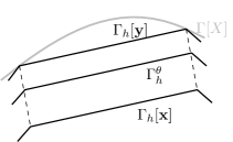
Figure 1: The construction of the intermediate surfaces $\Gamma_{h}^{\theta}$

The following formulae relate the mass and stiffness matrices for the discrete surfaces $\Gamma_{h}[{\mathbf{x}}]$ and $\Gamma_{h}[{\mathbf{y}}]$. They result from the Leibniz rule and are given in Lemma 4.1 of KLLP (17).

Lemma 3

In the above setting, the following identities hold true:

$${\mathbf{w}}^{T}({\mathbf{M}}({\mathbf{x}})-{\mathbf{M}}({\mathbf{y}})){\mathbf{z}}= \ \int_{0}^{1}\int_{\Gamma_{h}^{\theta}}w_{h}^{\theta}(\nabla_{\Gamma_{h}^{\theta}}\cdot e_{h}^{\theta})z_{h}^{\theta}\;\hbox{\rm{d}}\theta,$$ (28)

$${\mathbf{w}}^{T}({\mathbf{A}}({\mathbf{x}})-{\mathbf{A}}({\mathbf{y}})){\mathbf{z}}= \ \int_{0}^{1}\int_{\Gamma_{h}^{\theta}}\nabla_{\Gamma_{h}^{\theta}}w_{h}^{\theta}\cdot(D_{\Gamma_{h}^{\theta}}e_{h}^{\theta})\nabla_{\Gamma_{h}^{\theta}}z_{h}^{\theta}\;\hbox{\rm{d}}\theta,$$ (29)

where $D_{\Gamma_{h}^{\theta}}e_{h}^{\theta}=\textnormal{tr}(E^{\theta})I_{3}-(E^{\theta}+(E^{\theta})^{T})$ with $E^{\theta}=\nabla_{\Gamma_{h}^{\theta}}e_{h}^{\theta}\in\mathbb{R}^{3\times 3}$.

The following lemma combines Lemmas 4.2 and 4.3 of KLLP (17).

Lemma 4

In the above setting, if

$$\|\nabla_{\Gamma_{h}[{\mathbf{y}}]}e_{h}^{0}\|_{L^{\infty}(\Gamma_{h}[{\mathbf{y}}])}\leq\tfrac{1}{2},$$

then, for $0\leq\theta\leq 1$ and $1\leq p\leq\infty$, the finite element function
$w_{h}^{\theta}=\sum_{j=1}^{N}w_{j}\phi_{j}[{\mathbf{y}}+\theta{\mathbf{e}}]$ on $\Gamma_{h}^{\theta}=\Gamma_{h}[{\mathbf{y}}+\theta{\mathbf{e}}]$ is bounded by

$$\|w_{h}^{\theta}\|_{L^{p}(\Gamma_{h}^{\theta})}\leq c_{p}\,\|w_{h}^{0}\|_{L^{p}(\Gamma_{h}^{0})},$$

$$\|\nabla_{\Gamma_{h}^{\theta}}w_{h}^{\theta}\|_{L^{p}(\Gamma_{h}^{\theta})}\leq c_{p}\,\|\nabla_{\Gamma_{h}^{0}}w_{h}^{0}\|_{L^{p}(\Gamma_{h}^{0})},$$

where $c_{p}$ is an absolute constant (in particular, independent of $0\leq\theta\leq 1$ and $h$). Moreover, $c_{\infty}=2$.

The first estimate is not stated explicitly in KLLP (17), but follows immediately with the proof of Lemma 4.3 in KLLP (17).

If $\|\nabla_{\Gamma_{h}[{\mathbf{y}}]}e_{h}^{0}\|_{L^{\infty}(\Gamma_{h}[{\mathbf{y}}])}\leq\frac{1}{4}$, using the lemma for $w_{h}^{\theta}=e_{h}^{\theta}$ shows that

$$\|\nabla_{\Gamma_{h}^{\theta}}e_{h}^{\theta}\|_{L^{\infty}(\Gamma_{h}^{\theta})}\leq\tfrac{1}{2},\qquad 0\leq\theta\leq 1,$$ (30)

and then the lemma with $p=2$ and the definition of the norms (25) and (26) (and interchanging the roles of ${\mathbf{y}}$ and ${\mathbf{y}}+\theta{\mathbf{e}}$) show that

the norms $$\|\cdot\|_{{\mathbf{M}}({\mathbf{y}}+\theta{\mathbf{e}})} h 0\leq\theta\leq 1$$ are -uniformly equivalent for , (31)

and so are the norms $$\|\cdot\|_{{\mathbf{A}}({\mathbf{y}}+\theta{\mathbf{e}})}$$.

Under the condition that $\varepsilon:=\|\nabla_{\Gamma_{h}[{\mathbf{y}}]}e_{h}^{0}\|_{L^{\infty}(\Gamma_{h}[{\mathbf{y}}])}\leq\tfrac{1}{4}$, using (30) in Lemma 3 and applying the Cauchy-Schwarz inequality yields the bounds, with $c=c_{\infty}c_{2}^{2}$,

$${\mathbf{w}}^{T}({\mathbf{M}}({\mathbf{x}})-{\mathbf{M}}({\mathbf{y}})){\mathbf{z}}\leq \ c\varepsilon\,\|{\mathbf{w}}\|_{{\mathbf{M}}({\mathbf{y}})}\|{\mathbf{z}}\|_{{\mathbf{M}}({\mathbf{y}})},$$ (32)

$${\mathbf{w}}^{T}({\mathbf{A}}({\mathbf{x}})-{\mathbf{A}}({\mathbf{y}})){\mathbf{z}}\leq \ c\varepsilon\,\|{\mathbf{w}}\|_{{\mathbf{A}}({\mathbf{y}})}\|{\mathbf{z}}\|_{{\mathbf{A}}({\mathbf{y}})}.$$

We will also use similar bounds where we use the $L^{\infty}$ norm of $z_{h}$ or its gradient and the $L^{2}$ norm of the gradient of $e_{h}$:

$${\mathbf{w}}^{T}({\mathbf{M}}({\mathbf{x}})-{\mathbf{M}}({\mathbf{y}})){\mathbf{z}}\leq \ c\,\|{\mathbf{w}}\|_{{\mathbf{M}}({\mathbf{y}})}\|{\mathbf{e}}\|_{{\mathbf{A}}({\mathbf{y}})},$$ (33)

$${\mathbf{w}}^{T}({\mathbf{A}}({\mathbf{x}})-{\mathbf{A}}({\mathbf{y}})){\mathbf{z}}\leq \ c\,\|{\mathbf{w}}\|_{{\mathbf{A}}({\mathbf{y}})}\|{\mathbf{e}}\|_{{\mathbf{A}}({\mathbf{y}})}.$$

Consider now a continuously differentiable function ${\mathbf{x}}:[0,T]\rightarrow\mathbb{R}^{3N}$ that defines a finite element surface $\Gamma_{h}[{\mathbf{x}}(t)]$ for every $t\in[0,T]$, and assume that its time derivative ${\mathbf{v}}(t)=\dot{\mathbf{x}}(t)$ is the nodal vector of a finite element function $v_{h}(\cdot,t)$ that satisfies

$$\|\nabla_{\Gamma_{h}[{\mathbf{x}}(t)]}v_{h}(\cdot,t)\|_{L^{\infty}(\Gamma_{h}[{\mathbf{x}}(t)])}\leq K,\qquad 0\leq t\leq T.$$ (34)

With ${\mathbf{e}}={\mathbf{x}}(t)-{\mathbf{x}}(s)=\int_{s}^{t}{\mathbf{v}}(r)\,dr$, the bounds (32) then yield the following bounds, which were first shown in Lemma 4.1 of DLM (12):

for $0\leq s,t\leq T$ with $K|t-s|\leq\tfrac{1}{4}$, we have with $C=cK$

$${\mathbf{w}}^{T}\bigl{(}{\mathbf{M}}({\mathbf{x}}(t))-{\mathbf{M}}({\mathbf{x}}(s))\bigr{)}{\mathbf{z}}\leq \ C\,|t-s|\,\|{\mathbf{w}}\|_{{\mathbf{M}}({\mathbf{x}}(t))}\|{\mathbf{z}}\|_{{\mathbf{M}}({\mathbf{x}}(t))},$$ (35)

$${\mathbf{w}}^{T}\bigl{(}{\mathbf{A}}({\mathbf{x}}(t))-{\mathbf{A}}({\mathbf{x}}(s))\bigr{)}{\mathbf{z}}\leq \ C\,|t-s|\,\|{\mathbf{w}}\|_{{\mathbf{A}}({\mathbf{x}}(t))}\|{\mathbf{z}}\|_{{\mathbf{A}}({\mathbf{x}}(t))}.$$

Letting $s\rightarrow t$, this implies the bounds stated in Lemma 4.6 of KLLP (17):

$${\mathbf{w}}^{T}\frac{\hbox{\rm{d}}}{\hbox{\rm{d}}t}{\mathbf{M}}({\mathbf{x}}(t)){\mathbf{z}}\leq \ C\,\|{\mathbf{w}}\|_{{\mathbf{M}}({\mathbf{x}}(t))}\|{\mathbf{z}}\|_{{\mathbf{M}}({\mathbf{x}}(t))},$$ (36)

$${\mathbf{w}}^{T}\frac{\hbox{\rm{d}}}{\hbox{\rm{d}}t}{\mathbf{A}}({\mathbf{x}}(t)){\mathbf{z}}\leq \ C\,\|{\mathbf{w}}\|_{{\mathbf{A}}({\mathbf{x}}(t))}\|{\mathbf{z}}\|_{{\mathbf{A}}({\mathbf{x}}(t))}.$$

Moreover, by patching together finitely many intervals over which $K|t-s|\leq\tfrac{1}{4}$, we obtain that

the norms $$\|\cdot\|_{{\mathbf{M}}({\mathbf{x}}(t))} h 0\leq t\leq T$$ are -uniformly equivalent for , (37)

and so are the norms $$\|\cdot\|_{{\mathbf{A}}({\mathbf{x}}(t))}$$.

5.2 Preparation: Interpolation of products of finite element functions

For the stability of the velocity approximation we will need the following result.

Lemma 5

For an admissible triangulation of a smooth surface $\Gamma$, let $\Gamma_{h}^{*}$ be the interpolated surface with finite elements of polynomial degree $k\geq 1$. Let $\widetilde{I}_{h}^{*}:C(\Gamma_{h}^{*})\rightarrow S_{h}(\Gamma_{h}^{*})$ denote the finite element interpolation operator on $\Gamma_{h}^{*}$. Then, the interpolation of the product of two finite element functions $a_{h},b_{h}$ on $\Gamma_{h}^{*}$ is bounded by

$$\|\widetilde{I}_{h}^{*}(a_{h}b_{h})\|_{H^{1}(\Gamma_{h}^{*})}\leq C\,\|a_{h}\|_{H^{1}(\Gamma_{h}^{*})}\,\|b_{h}\|_{W^{1,\infty}(\Gamma_{h}^{*})},$$

where $C$ depends only on $\Gamma$ (more precisely, on bounds of higher derivatives of a parametrization of $\Gamma$), on shape-regularity and quasi-uniformity of the triangulation, and on the degree $k$.

Proof

Let $K$ be a curved triangle of the triangulation $\Gamma_{h}^{*}$. Using the interpolation error estimate of (Dem, 09, Proposition 2.7), on the element $K$ we obtain (with different constants $c$)

$$\|\widetilde{I}_{h}^{*}(a_{h}b_{h})-a_{h}b_{h}\|_{H^{1}(K)}\leq ch^{k}\|a_{h}b_{h}\|_{H^{k+1}(K)}\leq ch^{k}\sum_{j=0}^{k+1}|a_{h}b_{h}|_{H^{j}(K)}$$

$$\leq ch^{k}\sum_{j=0}^{k+1}\sum_{i=0}^{j}\|\nabla_{\Gamma_{h}}^{i}a_{h}\|_{L^{2}(K)}\|\nabla_{\Gamma_{h}}^{j-i}b_{h}\|_{L^{\infty}(K)}$$

$$=c\sum_{j=0}^{k}h^{k-j}\sum_{i=0}^{j}h^{i}\|\nabla_{\Gamma_{h}}^{i}a_{h}\|_{L^{2}(K)}\,h^{j-i}\|\nabla_{\Gamma_{h}}^{j-i}b_{h}\|_{L^{\infty}(K)}$$

$$\ \ +c\!\sum_{i=0}^{k}\!h^{i}\|\nabla_{\Gamma_{h}}^{i}a_{h}\|_{L^{2}(K)}\,h^{k-i}\|\nabla_{\Gamma_{h}}^{k+1-i}b_{h}\|_{L^{\infty}(K)}+ch^{k}\|\nabla_{\Gamma_{h}}^{k+1}a_{h}\|_{L^{2}(K)}\|b_{h}\|_{L^{\infty}(K)}.$$

By inverse estimates, this is further bounded by

$$\|\widetilde{I}_{h}^{*}(a_{h}b_{h})-a_{h}b_{h}\|_{H^{1}(K)}\leq c\|a_{h}\|_{L^{2}(K)}\|b_{h}\|_{L^{\infty}(K)}$$

$$\quad\ +c\|a_{h}\|_{L^{2}(K)}\|\nabla_{\Gamma_{h}}b_{h}\|_{L^{\infty}(K)}+c\|\nabla_{\Gamma_{h}}a_{h}\|_{L^{2}(K)}\|b_{h}\|_{L^{\infty}(K)}$$

$$\leq c\,\|a_{h}\|_{H^{1}(K)}\|b_{h}\|_{W^{1,\infty}(K)}$$

Squaring and summing up over the triangles then shows that

$$\|\widetilde{I}_{h}^{*}(a_{h}b_{h})-a_{h}b_{h}\|_{H^{1}(\Gamma_{h}^{*})}\leq c\|a_{h}\|_{H^{1}(\Gamma_{h}^{*})}\,\|b_{h}\|_{W^{1,\infty}(\Gamma_{h}^{*})}.$$

The stated result then follows with the triangle inequality. ∎

5.3 Defects and errors

We choose reference finite element functions $x_{h}^{*}(\cdot,t)$, $v_{h}^{*}(\cdot,t)$, $u_{h}^{*}(\cdot,t),w_{h}^{*}(\cdot,t)$ on the interpolated surface $\Gamma_{h}[{\mathbf{x}}^{\ast}(t)]$ with nodal vectors

$${\mathbf{x}}^{\ast}(t)\in\mathbb{R}^{3N},\ \ {\mathbf{v}}^{\ast}(t)\in\mathbb{R}^{3N},$$

$${\mathbf{u}}^{\ast}(t)=\begin{pmatrix}{\mathbf{H}}^{\ast}(t)\\ \mathbf{n}^{\ast}(t)\end{pmatrix}\in\mathbb{R}^{4N},\quad{\mathbf{w}}^{\ast}(t)=\begin{pmatrix}{\mathbf{V}}^{\ast}(t)\\ \mathbf{z}^{\ast}(t)\end{pmatrix}\in\mathbb{R}^{4N},$$

which are related to the exact solution $X$, $v$ and $u=(H,\nu)$, $w=(V,z)$ as follows: ${\mathbf{x}}^{\ast}(t)$ and ${\mathbf{v}}^{\ast}(t)$ collect the values at the finite element nodes of $X(\cdot,t)$ and $v(\cdot,t)$, respectively. The vectors ${\mathbf{u}}^{\ast}(t)$ and ${\mathbf{w}}^{\ast}(t)$ need to be chosen in a different way. The vector ${\mathbf{u}}^{\ast}(t)$ contains the nodal values of the finite element function $u_{h}^{*}(\cdot,t)\in S_{h}[{\mathbf{x}}^{\ast}(t)]^{4}$ that is determined on the interpolated surface $\Gamma_{h}[{\mathbf{x}}^{\ast}(t)]$ by a modified Ritz map of the exact solution component $u$ that will be defined in Section 6. Similarly, the vector ${\mathbf{w}}^{\ast}(t)$ contains the nodal values of the finite element function $w_{h}^{*}(\cdot,t)\in S_{h}[{\mathbf{x}}^{\ast}(t)]^{4}$ that is defined on the interpolated surface $\Gamma_{h}[{\mathbf{x}}^{\ast}(t)]$ by the Ritz map of the solution component $w$.

The nodal vectors ${\mathbf{x}}^{\ast}(t)$, ${\mathbf{v}}^{\ast}(t)$ then satisfy the equations (20) up to some defect ${\mathbf{d}}_{\mathbf{v}}$ that will be studied in Section 6,

$$\dot{\mathbf{x}}^{\ast} ={\mathbf{v}}^{\ast},$$ (38a)

$${\mathbf{v}}^{\ast} =\mathbf{V}^{\ast}\bullet\mathbf{n}^{\ast}+{\mathbf{d}}_{\mathbf{v}},$$ (38b)

and ${\mathbf{u}}^{\ast}(t)$, ${\mathbf{w}}^{\ast}(t)$ satisfy the equations (21) up to some defects ${\mathbf{d}}_{\bf u}$ and ${\mathbf{d}}_{\bf w}$ that will also be studied in Section 6:

$${\mathbf{M}}^{[4]}({\mathbf{x}}^{\ast})\dot{\mathbf{u}}^{\ast}-{\mathbf{A}}^{[4]}({\mathbf{x}}^{\ast}){\mathbf{w}}^{\ast}= \ {\mathbf{F}}({\mathbf{x}}^{\ast},{\mathbf{u}}^{\ast}){\mathbf{w}}^{\ast}+{\mathbf{f}}({\mathbf{x}}^{\ast},{\mathbf{u}}^{\ast})+{\mathbf{M}}^{[4]}({\mathbf{x}}^{\ast}){\mathbf{d}}_{\mathbf{u}},$$ (39a)

$${\mathbf{M}}^{[4]}({\mathbf{x}}^{\ast}){\mathbf{w}}^{\ast}+{\mathbf{A}}^{[4]}({\mathbf{x}}^{\ast}){\mathbf{u}}^{\ast}= \ {\mathbf{g}}({\mathbf{x}}^{\ast},{\mathbf{u}}^{\ast})+{\mathbf{M}}^{[4]}({\mathbf{x}}^{\ast}){\mathbf{d}}_{\mathbf{w}}.$$ (39b)

In the following we omit the superscript $[4]$ on ${\mathbf{M}}$ and ${\mathbf{A}}$. Furthermore, we simplify the notation and abbreviate ${\mathbf{M}}({\mathbf{x}}(t))$ and ${\mathbf{M}}({\mathbf{x}}^{\ast}(t))$ to ${\mathbf{M}}(t)$ and ${\mathbf{M}}^{\ast}(t)$, respectively. Similarly we write ${\mathbf{A}}$ and ${\mathbf{A}}^{\ast}$.

The errors between the nodal values of the numerical solutions and the nodal values of the interpolated exact values are denoted by ${\mathbf{e}}_{\mathbf{x}}={\mathbf{x}}-{\mathbf{x}}^{\ast}$, ${\mathbf{e}}_{\mathbf{v}}={\mathbf{v}}-{\mathbf{v}}^{\ast}$, ${\mathbf{e}}_{\mathbf{u}}={\mathbf{u}}-{\mathbf{u}}^{\ast}$ and ${\mathbf{e}}_{\mathbf{w}}={\mathbf{w}}-{\mathbf{w}}^{\ast}$ and their corresponding finite element functions on the interpolated surface $\Gamma_{h}[{\mathbf{x}}^{\ast}]$ are denoted by $e_{x}$, $e_{v}$, $e_{u}$, and $e_{w}$, respectively.

We obtain the error equations by subtracting (39) from (21) with (23) instead of (21b), and (38) from (20):

$$\dot{\mathbf{e}}_{\mathbf{x}}= \ {\mathbf{e}}_{\mathbf{v}},$$ (40a)

$${\mathbf{e}}_{\mathbf{v}}= \ \mathbf{V}\bullet\mathbf{n}-\mathbf{V}^{\ast}\bullet\mathbf{n}^{\ast}-{\mathbf{d}}_{\mathbf{v}},$$ (40b)

$${\mathbf{M}}\dot{\mathbf{e}}_{\mathbf{u}}-{\mathbf{A}}{\mathbf{e}}_{\mathbf{w}}= \ -\big{(}{\mathbf{M}}-{\mathbf{M}}^{\ast}\big{)}\dot{\mathbf{u}}^{\ast}+\big{(}{\mathbf{A}}-{\mathbf{A}}^{\ast}\big{)}{\mathbf{w}}^{\ast}$$

$$\ +\big{(}{\mathbf{F}}({\mathbf{x}},{\mathbf{u}}){\mathbf{w}}-{\mathbf{F}}({\mathbf{x}}^{\ast},{\mathbf{u}}^{\ast}){\mathbf{w}}^{\ast}\big{)}$$

$$\ +\big{(}{\mathbf{f}}({\mathbf{x}},{\mathbf{u}})-{\mathbf{f}}({\mathbf{x}}^{\ast},{\mathbf{u}}^{\ast})\big{)}-{\mathbf{M}}^{\ast}{\mathbf{d}}_{\mathbf{u}},$$ (40c)

$${\mathbf{M}}{\mathbf{e}}_{\mathbf{w}}+{\mathbf{A}}{\mathbf{e}}_{\mathbf{u}}= \ -\big{(}{\mathbf{M}}-{\mathbf{M}}^{\ast}\big{)}{\mathbf{w}}^{\ast}-\big{(}{\mathbf{A}}-{\mathbf{A}}^{\ast}\big{)}{\mathbf{u}}^{\ast}$$

$$\ +\big{(}{\mathbf{g}}({\mathbf{x}},{\mathbf{u}})-{\mathbf{g}}({\mathbf{x}}^{\ast},{\mathbf{u}}^{\ast})\big{)}-{\mathbf{M}}^{\ast}{\mathbf{d}}_{\mathbf{w}}+{\bm{\vartheta}}.$$ (40d)

We note further that ${\mathbf{e}}_{\mathbf{x}}(0)=0$, but in general ${\mathbf{e}}_{\mathbf{v}}(0)$, ${\mathbf{e}}_{\mathbf{u}}(0)$ and ${\mathbf{e}}_{\mathbf{w}}(0)$ are different from $0$. We recall from (22) that

$${\bm{\vartheta}}={\mathbf{M}}({\mathbf{x}}(0))\,{\bar{\mathbf{e}}}_{\mathbf{w}}(0)\quad\text{ with }\quad{\bar{\mathbf{e}}}_{\mathbf{w}}(0)=\bar{\mathbf{w}}^{*}(0)-\bar{\mathbf{w}}(0).$$

This is not to be confounded with ${\mathbf{e}}_{\mathbf{w}}(0)=\bar{\mathbf{w}}^{*}(0)-{\mathbf{w}}^{*}(0)$, where we remind that $\bar{\mathbf{w}}^{*}(0)$ contains the values of the exact solution $w$ in the nodes, whereas ${\mathbf{w}}^{*}(0)$ is constructed by a Ritz map from the exact solution $w$ at the initial time $0$.

5.4 Stability estimate

We need to bound the errors at time $t$ in terms of the defects up to time $t$ and the errors in the initial values. The errors will be estimated in the $H^{1}$ norm on the interpolated surface $\Gamma_{h}[{\mathbf{x}}^{\ast}]$: for a nodal vector ${\mathbf{e}}$ corresponding to a finite element function $e\in S_{h}({\mathbf{x}}^{*})$, we have with the matrix ${\mathbf{K}}({\mathbf{x}}^{\ast})={\mathbf{M}}({\mathbf{x}}^{\ast})+{\mathbf{A}}({\mathbf{x}}^{\ast})$ that

$$\|{\mathbf{e}}\|_{{\mathbf{K}}({\mathbf{x}}^{\ast})}^{2}={\mathbf{e}}^{T}{\mathbf{K}}({\mathbf{x}}^{\ast}){\mathbf{e}}=\|e\|_{H^{1}(\Gamma_{h}[{\mathbf{x}}^{\ast}])}^{2}.$$

The defect ${\mathbf{d}}_{\mathbf{v}}$ then needs to be sufficiently small in the $H^{1}$ norm, and the other defects will be required to be small in the $L^{2}$ norm

$$\|{\mathbf{d}}\|_{{\mathbf{M}}({\mathbf{x}}^{\ast})}^{2}={\mathbf{d}}^{T}{\mathbf{M}}({\mathbf{x}}^{\ast}){\mathbf{d}}=\|d\|_{L^{2}(\Gamma_{h}[{\mathbf{x}}^{\ast}])}^{2},$$

and their time derivatives as well as ${\bar{\mathbf{e}}}_{\mathbf{w}}(0)$ will be required to be small in the norm given by

$$\|{\mathbf{d}}\|_{\star,{\mathbf{x}}^{\ast}}^{2}:={\mathbf{d}}^{T}{\mathbf{M}}({\mathbf{x}}^{\ast}){\mathbf{K}}({\mathbf{x}}^{\ast})^{-1}{\mathbf{M}}({\mathbf{x}}^{\ast}){\mathbf{d}}.$$

By (KLLP, 17, Eq. (5.5)), this equals the following dual norm for the corresponding finite element function $d\in S_{h}[{\mathbf{x}}^{*}]$, which has the vector of nodal values ${\mathbf{d}}$,

$$\|{\mathbf{d}}\|_{\star,{\mathbf{x}}^{\ast}}=\|d\|_{H_{h}^{-1}(\Gamma_{h}[{\mathbf{x}}^{*}])}:=\sup_{0\neq\varphi_{h}\in S_{h}[{\mathbf{x}}^{\ast}]}\frac{\int_{\Gamma_{h}[{\mathbf{x}}^{\ast}]}d\cdot\varphi_{h}}{\|\varphi_{h}\|_{H^{1}(\Gamma_{h}[{\mathbf{x}}^{\ast}])}}\,.$$

The following result provides the key stability estimate, which bounds the errors in terms of the defects and the initial errors.

Proposition 1

Assume that the reference finite element functions $x_{h}^{*}(\cdot,t)$, $v_{h}^{*}(\cdot,t)$, $u_{h}^{*}(\cdot,t),w_{h}^{*}(\cdot,t)$ on the interpolated surface $\Gamma_{h}[{\mathbf{x}}^{\ast}(t)]$ have $W^{1,\infty}$ norms that are bounded independently of $h$, for all $t\in[0,T]$. Assume that, for some $\kappa$ with $1<\kappa\leq k$, the defects are bounded by

$$\begin{aligned} \|{\mathbf{d}}_{\mathbf{v}}(t)\|_{{\mathbf{K}}({\mathbf{x}}^{\ast}(t))}\leq&\ ch^{\kappa},\\ \|{\mathbf{d}}_{\mathbf{u}}(t)\|_{{\mathbf{M}}({\mathbf{x}}^{\ast}(t))}+\|\dot{\mathbf{d}}_{\mathbf{u}}(t)\|_{\star,{\mathbf{x}}^{\ast}(t)}\leq&\ ch^{\kappa},\\ \|{\mathbf{d}}_{\mathbf{w}}(t)\|_{{\mathbf{M}}({\mathbf{x}}^{\ast}(t))}+\|\dot{\mathbf{d}}_{\mathbf{w}}(t)\|_{\star,{\mathbf{x}}^{\ast}(t)}\leq&\ ch^{\kappa},\\ \end{aligned}\qquad\hbox{for }\ 0\leq t\leq T,$$ (41)

and that the errors of the initial values are bounded by

$$\|{\mathbf{e}}_{\mathbf{u}}(0)\|_{{\mathbf{K}}({\mathbf{x}}^{0})}+\|{\mathbf{e}}_{\mathbf{w}}(0)\|_{{\mathbf{K}}({\mathbf{x}}^{0})} \leq ch^{\kappa},$$ (42)

$$\|{\bar{\mathbf{e}}}_{\mathbf{w}}(0)\|_{\star,{\mathbf{x}}^{0}} \leq ch^{\kappa}.$$

Then, there exists $h_{0}>0$ such that the following stability estimate holds for all $h\leq h_{0}$ and $0\leq t\leq T$:

$$\|{\mathbf{e}}_{\mathbf{x}}(t)\|_{{\mathbf{K}}({\mathbf{x}}^{\ast}(t))}^{2}+\|{\mathbf{e}}_{\mathbf{v}}(t)\|_{{\mathbf{K}}({\mathbf{x}}^{\ast}(t))}^{2}+\|{\mathbf{e}}_{\mathbf{u}}(t)\|_{{\mathbf{K}}({\mathbf{x}}^{\ast}(t))}^{2}+\|{\mathbf{e}}_{\mathbf{w}}(t)\|_{{\mathbf{K}}({\mathbf{x}}^{\ast}(t))}^{2}$$ (43)

$$\leq \ C\max_{0\leq s\leq t}\big{(}\|{\mathbf{d}}_{\mathbf{v}}(s)\|_{{\mathbf{K}}({\mathbf{x}}^{\ast}(s))}^{2}+\|{\mathbf{d}}_{\mathbf{u}}(s)\|_{\star,{\mathbf{x}}^{\ast}(s)}^{2}\big{)}$$

$$\ +C\!\int_{0}^{t}\!\Big{(}\|{\mathbf{d}}_{\mathbf{u}}(s)\|_{{\mathbf{M}}({\mathbf{x}}^{\ast}(s))}^{2}+\|\dot{\mathbf{d}}_{\mathbf{u}}(s)\|_{\star,{\mathbf{x}}^{\ast}(s)}^{2}$$

$$\ \phantom{+C\!\int_{0}^{t}\!\Big{(}\ }+\|{\mathbf{d}}_{\mathbf{w}}(s)\|_{{\mathbf{M}}({\mathbf{x}}^{\ast}(s))}^{2}+\|\dot{\mathbf{d}}_{\mathbf{w}}(s)\|_{\star,{\mathbf{x}}^{\ast}(s)}^{2}\Big{)}\hbox{\rm{d}}s$$

$$\ +C\bigl{(}\|{\mathbf{e}}_{\mathbf{u}}(0)\|_{{\mathbf{K}}({\mathbf{x}}^{0})}^{2}+\|{\mathbf{e}}_{\mathbf{w}}(0)\|_{{\mathbf{K}}({\mathbf{x}}^{0})}^{2}\bigr{)}+C\|{\bar{\mathbf{e}}}_{\mathbf{w}}(0)\|_{\star,{\mathbf{x}}^{0}}^{2},$$

where $C$ is independent of $h$ and $t$, but depends on the final time $T$.

Proof

The proof uses energy estimates for the error equations in the matrix–vector formulation (40) and relies on the lemmas of Section 5.1, which relate the different finite element surfaces. While this basic procedure of the proof looks similar to that of KLL (19) and KLLP (17), there are substantial differences and technical difficulties that are peculiar to the fourth-order system.

We exploit the skew-symmetric structure of the system of error equations (40)–(40). The uniform-in-time stability estimate follows from the combination of four different sets of auxiliary energy estimates (denoted by (i)–(iv)), divided into two major parts, Parts (A.1) and (A.2), and finally combining them in Part (A.3), which gives the uniform-in-time stability bound for the errors ${\mathbf{e}}_{\mathbf{u}}$ and ${\mathbf{e}}_{\mathbf{w}}$, as illustrated in Figure 2. Part (B) of the proof contains the estimates for the velocity error equation (40b), and finally the two are combined in Part (C), to show the stability bound (43).

Figure 2: Sketch of the structure of the energy estimates of Part (A) for the stability proof. In the diagram, ${\mathbf{r}}_{1}$ and ${\mathbf{r}}_{2}$ denote the right-hand sides of (40) and (40), respectively. (Note that, after time differentiation, ${\mathbf{R}}_{2}$ contains terms other than only the time derivative of ${\mathbf{r}}_{2}$.)

Let $t^{*}\in(0,T]$ be the maximal time such that the following inequalities hold:

$$\begin{aligned} \|e_{x}(\cdot,t)\|_{W^{1,\infty}(\Gamma_{h}[{\mathbf{x}}^{\ast}(t)])}\leq&\ h^{(\kappa-1)/2},\\ \|e_{v}(\cdot,t)\|_{W^{1,\infty}(\Gamma_{h}[{\mathbf{x}}^{\ast}(t)])}\leq&\ h^{(\kappa-1)/2},\\ \|e_{u}(\cdot,t)\|_{W^{1,\infty}(\Gamma_{h}[{\mathbf{x}}^{\ast}(t)])}\leq&\ h^{(\kappa-1)/2},\\ \|e_{w}(\cdot,t)\|_{W^{1,\infty}(\Gamma_{h}[{\mathbf{x}}^{\ast}(t)])}\leq&\ h^{(\kappa-1)/2},\end{aligned}\qquad\textrm{ for }\quad t\in[0,t^{*}].$$ (44)

Note that $t^{*}>0$ since initially $e_{x}(\cdot,0)=0$ and, by an inverse inequality, we have

$$\|e_{u}(\cdot,0)\|_{W^{1,\infty}(\Gamma_{h}[{\mathbf{x}}^{\ast}(0)])} \leq ch^{-1}\|e_{u}(\cdot,0)\|_{H^{1}(\Gamma_{h}[{\mathbf{x}}^{\ast}(0)])}$$

$$=ch^{-1}\|{\mathbf{e}}_{\mathbf{u}}(0)\|_{{\mathbf{K}}({\mathbf{x}}^{\ast}(t))}\leq Ch^{\kappa-1},$$

where the last inequality holds by assumption (42). By the same argument, also $\|e_{w}(\cdot,0)\|_{W^{1,\infty}(\Gamma_{h}[{\mathbf{x}}^{\ast}(0)])}\leq Ch^{\kappa-1}$ and, as a result of $v_{h}=\widetilde{I}_{h}(V_{h}\nu_{h})$,

$$\|e_{v}(\cdot,0)\|_{W^{1,\infty}(\Gamma_{h}[{\mathbf{x}}^{\ast}(0)])}$$

$$\leq c\|e_{u}(\cdot,0)\|_{W^{1,\infty}(\Gamma_{h}[{\mathbf{x}}^{\ast}(0)])}+c\|e_{w}(\cdot,0)\|_{W^{1,\infty}(\Gamma_{h}[{\mathbf{x}}^{\ast}(0)])}\leq Ch^{\kappa-1}.$$

By continuity, we then obtain for sufficiently small $h$ that $t^{*}>0$ (which a priori might depend on $h$). We first prove the stated error bounds for $0\leq t\leq t^{*}$. At the end of the proof we will show that in fact $t^{*}$ coincides with $T$.

Since the reference finite element functions $x_{h}^{*}(\cdot,t),v_{h}^{*}(\cdot,t),u_{h}^{*}(\cdot,t),w_{h}^{*}(\cdot,t)$ on the interpolated surface $\Gamma_{h}[{\mathbf{x}}^{\ast}(t)]$ have $W^{1,\infty}$ norms that are bounded independently of $h$ for all $t\in[0,T]$, the bounds (44) together with Lemma 4 imply that the $W^{1,\infty}$ norms of the ESFEM functions $x_{h}(\cdot,t),v_{h}(\cdot,t),u_{h}(\cdot,t)$, $w_{h}(\cdot,t)$ on the discrete surface $\Gamma_{h}[{\mathbf{x}}(t)]$ are also bounded independently of $h$ and $t\in[0,t^{*}]$, and so are their lifts to the interpolated surface $\Gamma_{h}[{\mathbf{x}}^{\ast}(t)]$. In particular, it will be important that the discrete velocity $v_{h}$ with nodal vector ${\mathbf{v}}$ satisfies (34).

The estimate on the position errors $e_{x}$ in (44) and the $W^{1,\infty}$ bound on $v_{h}$ immediately imply that the results of Section 5.1 apply with ${\mathbf{x}}$ and ${\mathbf{x}}^{\ast}$ in the roles of ${\mathbf{x}}$ and ${\mathbf{y}}$, respectively. In particular, due to the bounds in (44) (for a sufficiently small $h\leq h_{0}$), the main condition of Lemma 4 and also (30) is satisfied (with $e_{h}^{\theta}=e_{x}^{\theta}$), hence the $h$-uniform norm equivalences in (31) and the estimates in (32) and (33) hold between the surfaces defined by ${\mathbf{x}}$ and ${\mathbf{x}}^{\ast}$. Similarly, again due to (44) the bound (34) also holds, and hence the estimates in (35), (36) and the $h$-uniform norm equivalences in time (37) also hold. When referring to these results from Section 5.1 ((31)–(33), (35)–(37)) within the stability proof below, following the above argument, we always mean that their respective smallness assumptions are satisfied via (44), but we will not repeat this argument at each instance.

In the following $c$ and $C$ will denote generic constants that might take different values on different occurrences. In contrast, constants with a subscript (such as $c_{0}$) will play a distinctive role in the proof, and will not change their value between appearances.

(A) Estimates for the surface PDEs:

(A.1) We start by showing an error estimate for ${\mathbf{e}}_{\mathbf{u}}$ in the ${\mathbf{K}}$-norm uniformly in time for $0\leq t\leq t^{*}$. A critical term will appear, which will be controlled in Part (A.2) and eliminated in (A.3).

Energy estimate (i): We test (40) with ${\mathbf{e}}_{\mathbf{w}}$, and test (40) with $\dot{\mathbf{e}}_{\mathbf{u}}$, so that we obtain the two equations

$${\mathbf{e}}_{\mathbf{w}}^{T}{\mathbf{M}}\dot{\mathbf{e}}_{\mathbf{u}}-{\mathbf{e}}_{\mathbf{w}}^{T}{\mathbf{A}}{\mathbf{e}}_{\mathbf{w}}= \ -{\mathbf{e}}_{\mathbf{w}}^{T}\big{(}{\mathbf{M}}-{\mathbf{M}}^{\ast}\big{)}\dot{\mathbf{u}}^{\ast}+{\mathbf{e}}_{\mathbf{w}}^{T}\big{(}{\mathbf{A}}-{\mathbf{A}}^{\ast}\big{)}{\mathbf{w}}^{\ast}$$

$$\ +{\mathbf{e}}_{\mathbf{w}}^{T}\big{(}{\mathbf{F}}({\mathbf{x}},{\mathbf{u}}){\mathbf{w}}-{\mathbf{F}}({\mathbf{x}}^{\ast},{\mathbf{u}}^{\ast}){\mathbf{w}}^{\ast}\big{)}$$

$$\ +{\mathbf{e}}_{\mathbf{w}}^{T}\big{(}{\mathbf{f}}({\mathbf{x}},{\mathbf{u}})-{\mathbf{f}}({\mathbf{x}}^{\ast},{\mathbf{u}}^{\ast})\big{)}-{\mathbf{e}}_{\mathbf{w}}^{T}{\mathbf{M}}^{\ast}{\mathbf{d}}_{\mathbf{u}},$$

$$\dot{\mathbf{e}}_{\mathbf{u}}^{T}{\mathbf{M}}{\mathbf{e}}_{\mathbf{w}}+\dot{\mathbf{e}}_{\mathbf{u}}^{T}{\mathbf{A}}{\mathbf{e}}_{\mathbf{u}}= \ -\dot{\mathbf{e}}_{\mathbf{u}}^{T}\big{(}{\mathbf{M}}-{\mathbf{M}}^{\ast}\big{)}{\mathbf{w}}^{\ast}-\dot{\mathbf{e}}_{\mathbf{u}}^{T}\big{(}{\mathbf{A}}-{\mathbf{A}}^{\ast}\big{)}{\mathbf{u}}^{\ast}$$

$$\ +\dot{\mathbf{e}}_{\mathbf{u}}^{T}\big{(}{\mathbf{g}}({\mathbf{x}},{\mathbf{u}})-{\mathbf{g}}({\mathbf{x}}^{\ast},{\mathbf{u}}^{\ast})\big{)}-\dot{\mathbf{e}}_{\mathbf{u}}^{T}{\mathbf{M}}^{\ast}{\mathbf{d}}_{\mathbf{w}}+\dot{\mathbf{e}}_{\mathbf{u}}^{T}{\bm{\vartheta}},$$

In order to eliminate the mixed term ${\mathbf{e}}_{\mathbf{w}}^{T}{\mathbf{M}}\dot{\mathbf{e}}_{\mathbf{u}}$ (using the symmetry of the mass matrix ${\mathbf{M}}$), we then subtract the former equation from the latter, and obtain

$$\|{\mathbf{e}}_{\mathbf{w}}\|_{{\mathbf{A}}}^{2}+\dot{\mathbf{e}}_{\mathbf{u}}^{T}{\mathbf{A}}{\mathbf{e}}_{\mathbf{u}}= \ +{\mathbf{e}}_{\mathbf{w}}^{T}\big{(}{\mathbf{M}}-{\mathbf{M}}^{\ast}\big{)}\dot{\mathbf{u}}^{\ast}-{\mathbf{e}}_{\mathbf{w}}^{T}\big{(}{\mathbf{A}}-{\mathbf{A}}^{\ast}\big{)}{\mathbf{w}}^{\ast}$$ (45)

$$\ -{\mathbf{e}}_{\mathbf{w}}^{T}\big{(}{\mathbf{F}}({\mathbf{x}},{\mathbf{u}}){\mathbf{w}}-{\mathbf{F}}({\mathbf{x}}^{\ast},{\mathbf{u}}^{\ast}){\mathbf{w}}^{\ast}\big{)}$$

$$\ -{\mathbf{e}}_{\mathbf{w}}^{T}\big{(}{\mathbf{f}}({\mathbf{x}},{\mathbf{u}})-{\mathbf{f}}({\mathbf{x}}^{\ast},{\mathbf{u}}^{\ast})\big{)}+{\mathbf{e}}_{\mathbf{w}}^{T}{\mathbf{M}}^{\ast}{\mathbf{d}}_{\mathbf{u}},$$

$$\ -\dot{\mathbf{e}}_{\mathbf{u}}^{T}\big{(}{\mathbf{M}}-{\mathbf{M}}^{\ast}\big{)}{\mathbf{w}}^{\ast}-\dot{\mathbf{e}}_{\mathbf{u}}^{T}\big{(}{\mathbf{A}}-{\mathbf{A}}^{\ast}\big{)}{\mathbf{u}}^{\ast}$$

$$\ +\dot{\mathbf{e}}_{\mathbf{u}}^{T}\big{(}{\mathbf{g}}({\mathbf{x}},{\mathbf{u}})-{\mathbf{g}}({\mathbf{x}}^{\ast},{\mathbf{u}}^{\ast})\big{)}-\dot{\mathbf{e}}_{\mathbf{u}}^{T}{\mathbf{M}}^{\ast}{\mathbf{d}}_{\mathbf{w}}+\dot{\mathbf{e}}_{\mathbf{u}}^{T}{\bm{\vartheta}}.$$

The terms in equation (45) will now be bounded separately, using the results of Section 5.1.

For the second term on the left-hand side of (45), using the product rule, the symmetry of ${\mathbf{A}}$ and the bound (36), we have

$$\dot{\mathbf{e}}_{\mathbf{u}}^{T}{\mathbf{A}}{\mathbf{e}}_{\mathbf{u}}= \ \frac{1}{2}\frac{\hbox{\rm{d}}}{\hbox{\rm{d}}t}\Big{(}{\mathbf{e}}_{\mathbf{u}}^{T}{\mathbf{A}}{\mathbf{e}}_{\mathbf{u}}\Big{)}-\frac{1}{2}{\mathbf{e}}_{\mathbf{u}}^{T}\dot{\mathbf{A}}{\mathbf{e}}_{\mathbf{u}}$$ (46)

$$\geq \ \frac{1}{2}\frac{\hbox{\rm{d}}}{\hbox{\rm{d}}t}\|{\mathbf{e}}_{\mathbf{u}}\|_{{\mathbf{A}}}^{2}-c\|{\mathbf{e}}_{\mathbf{u}}\|_{{\mathbf{A}}}^{2}.$$

On the right-hand side, for the matrix difference terms in the first and fourth line of (45) we use (33), and, recalling that ${\mathbf{M}}^{\ast}+{\mathbf{A}}^{\ast}={\mathbf{K}}^{\ast}$, we obtain

$${\mathbf{e}}_{\mathbf{w}}^{T}\big{(}{\mathbf{M}}-{\mathbf{M}}^{\ast}\big{)}\dot{\mathbf{u}}^{\ast}-{\mathbf{e}}_{\mathbf{w}}^{T}\big{(}{\mathbf{A}}-{\mathbf{A}}^{\ast}\big{)}{\mathbf{w}}^{\ast}\leq \ c\|{\mathbf{e}}_{\mathbf{w}}\|_{{\mathbf{K}}}\|{\mathbf{e}}_{\mathbf{x}}\|_{{\mathbf{K}}},$$ (47)

$$-\dot{\mathbf{e}}_{\mathbf{u}}^{T}\big{(}{\mathbf{M}}-{\mathbf{M}}^{\ast}\big{)}{\mathbf{w}}^{\ast}-\dot{\mathbf{e}}_{\mathbf{u}}^{T}\big{(}{\mathbf{A}}-{\mathbf{A}}^{\ast}\big{)}{\mathbf{u}}^{\ast}\leq \ c\|\dot{\mathbf{e}}_{\mathbf{u}}\|_{{\mathbf{K}}}\|{\mathbf{e}}_{\mathbf{x}}\|_{{\mathbf{K}}}.$$

For the defect terms in (45), we obtain

$${\mathbf{e}}_{\mathbf{w}}^{T}{\mathbf{M}}^{\ast}{\mathbf{d}}_{\mathbf{u}} =\int_{\Gamma_{h}[{\mathbf{x}}^{\ast}]}\!\!e_{w}\,d_{u}$$

$$\leq\|e_{w}\|_{H^{1}(\Gamma_{h}[{\mathbf{x}}^{\ast}])}\,\|d_{u}\|_{H_{h}^{-1}(\Gamma_{h}[{\mathbf{x}}^{\ast}])}=\|{\mathbf{e}}_{\mathbf{w}}\|_{{\mathbf{K}}^{\ast}}\|{\mathbf{d}}_{\mathbf{u}}\|_{\star,{\mathbf{x}}^{\ast}}$$

and in the same way

$$-\dot{\mathbf{e}}_{\mathbf{u}}^{T}{\mathbf{M}}^{\ast}{\mathbf{d}}_{\mathbf{w}}\leq\|\dot{\mathbf{e}}_{\mathbf{u}}\|_{{\mathbf{K}}^{\ast}}\|{\mathbf{d}}_{\mathbf{w}}\|_{\star,{\mathbf{x}}^{\ast}},$$

and similarly, using the norm equivalence (37),

$$\dot{\mathbf{e}}_{\mathbf{u}}(t)^{T}{\bm{\vartheta}} =\dot{\mathbf{e}}_{\mathbf{u}}(t)^{T}{\mathbf{M}}({\mathbf{x}}^{0}){\bar{\mathbf{e}}}_{\mathbf{w}}^{0}$$

$$\leq\|\dot{\mathbf{e}}_{\mathbf{u}}(t)\|_{{\mathbf{K}}({\mathbf{x}}^{0})}\,\|{\bar{\mathbf{e}}}_{\mathbf{w}}^{0}\|_{\star,{\mathbf{x}}^{0}}\leq c\|\dot{\mathbf{e}}_{\mathbf{u}}(t)\|_{{\mathbf{K}}({\mathbf{x}}(t))}\,\|{\bar{\mathbf{e}}}_{\mathbf{w}}^{0}\|_{\star,{\mathbf{x}}^{0}}.$$

We thus obtain the following bounds for the defect terms:

$${\mathbf{e}}_{\mathbf{w}}^{T}{\mathbf{M}}^{\ast}{\mathbf{d}}_{\mathbf{u}}\leq \ c\|{\mathbf{e}}_{\mathbf{w}}\|_{{\mathbf{K}}}\|{\mathbf{d}}_{\mathbf{u}}\|_{\star,{\mathbf{x}}^{\ast}},$$ (48)

$$-\dot{\mathbf{e}}_{\mathbf{u}}^{T}{\mathbf{M}}^{\ast}{\mathbf{d}}_{\mathbf{w}}\leq \ c\|\dot{\mathbf{e}}_{\mathbf{u}}\|_{{\mathbf{K}}}\,\|{\mathbf{d}}_{\mathbf{w}}\|_{\star,{\mathbf{x}}^{\ast}},$$

$$\dot{\mathbf{e}}_{\mathbf{u}}^{T}{\bm{\vartheta}}\leq \ c\|\dot{\mathbf{e}}_{\mathbf{u}}\|_{{\mathbf{K}}}\,\|{\bar{\mathbf{e}}}_{\mathbf{w}}^{0}\|_{\star,{\mathbf{x}}^{0}}.$$

For the non-linear terms we use the following bounds: The two terms involving ${\mathbf{f}}$ and ${\mathbf{g}}$ are bounded exactly as the (general, locally Lipschitz) non-linear term in Part (A.v) in the proof of Proposition 7.1 in KLL (19) (using the fact that by the $W^{1,\infty}$ bound for the exact solution $u_{h}^{\ast}$ and the error $e_{u}$ in (44), the numerical solution $u_{h}$ is also bounded in the $W^{1,\infty}$ norm) and the norm equivalence (31). We altogether have

$${\mathbf{e}}_{\mathbf{w}}^{T}\big{(}{\mathbf{f}}({\mathbf{x}},{\mathbf{u}})-{\mathbf{f}}({\mathbf{x}}^{\ast},{\mathbf{u}}^{\ast})\big{)}\leq \ c\|{\mathbf{e}}_{\mathbf{w}}\|_{{\mathbf{K}}}\big{(}\|{\mathbf{e}}_{\mathbf{x}}\|_{{\mathbf{K}}}+\|{\mathbf{e}}_{\mathbf{u}}\|_{{\mathbf{K}}}\big{)}$$ (49)

$$\dot{\mathbf{e}}_{\mathbf{u}}^{T}\big{(}{\mathbf{g}}({\mathbf{x}},{\mathbf{u}})-{\mathbf{g}}({\mathbf{x}}^{\ast},{\mathbf{u}}^{\ast})\big{)}\leq \ c\|\dot{\mathbf{e}}_{\mathbf{u}}\|_{{\mathbf{M}}}\big{(}\|{\mathbf{e}}_{\mathbf{x}}\|_{{\mathbf{K}}}+\|{\mathbf{e}}_{\mathbf{u}}\|_{{\mathbf{K}}}\big{)}.$$

For the term involving the state-dependent mass matrix ${\mathbf{F}}({\mathbf{x}},{\mathbf{u}})$ we estimate by

$$\ -{\mathbf{e}}_{\mathbf{w}}^{T}\big{(}{\mathbf{F}}({\mathbf{x}},{\mathbf{u}}){\mathbf{w}}-{\mathbf{F}}({\mathbf{x}}^{\ast},{\mathbf{u}}^{\ast}){\mathbf{w}}^{\ast}\big{)}$$ (50)

$$= \ -{\mathbf{e}}_{\mathbf{w}}^{T}{\mathbf{F}}({\mathbf{x}},{\mathbf{u}}){\mathbf{e}}_{\mathbf{w}}-{\mathbf{e}}_{\mathbf{w}}^{T}\big{(}{\mathbf{F}}({\mathbf{x}},{\mathbf{u}})-{\mathbf{F}}({\mathbf{x}}^{\ast},{\mathbf{u}}^{\ast})\big{)}{\mathbf{w}}^{\ast}$$

$$\leq \ c_{0}\|{\mathbf{e}}_{\mathbf{w}}\|_{{\mathbf{M}}}^{2}+c\|{\mathbf{e}}_{\mathbf{w}}\|_{{\mathbf{M}}}\big{(}\|{\mathbf{e}}_{\mathbf{x}}\|_{{\mathbf{K}}}+\|{\mathbf{e}}_{\mathbf{u}}\|_{{\mathbf{K}}}\big{)},$$

where the first term in the middle line is estimated using (19) together with the $W^{1,\infty}$ boundedness of the numerical solutions $u_{h}$ (due to (44)), while the second term is again estimated using the above argument from (KLL, 19, Proposition 7.1, Part (A.v)), and using the norm equivalence (31). Here, $c_{0}$ is a positive constant.

Altogether, the combination of the above bounds yields the first energy estimate

$$\|{\mathbf{e}}_{\mathbf{w}}\|_{{\mathbf{A}}}^{2}+\frac{\hbox{\rm{d}}}{\hbox{\rm{d}}t}\|{\mathbf{e}}_{\mathbf{u}}\|_{{\mathbf{A}}}^{2}\leq \ c\|{\mathbf{e}}_{\mathbf{u}}\|_{{\mathbf{A}}}^{2}+2c_{0}\|{\mathbf{e}}_{\mathbf{w}}\|_{{\mathbf{M}}}^{2}$$ (51)

$$\ +c\|{\mathbf{e}}_{\mathbf{w}}\|_{{\mathbf{K}}}\big{(}\|{\mathbf{e}}_{\mathbf{x}}\|_{{\mathbf{K}}}+\|{\mathbf{e}}_{\mathbf{u}}\|_{{\mathbf{K}}}+\|{\mathbf{d}}_{\mathbf{u}}\|_{\star,{\mathbf{x}}^{\ast}}\big{)}$$

$$\ +c\|\dot{\mathbf{e}}_{\mathbf{u}}\|_{{\mathbf{K}}}\big{(}\|{\mathbf{e}}_{\mathbf{x}}\|_{{\mathbf{K}}}+\|{\mathbf{e}}_{\mathbf{u}}\|_{{\mathbf{K}}}+\|{\mathbf{d}}_{\mathbf{w}}\|_{\star,{\mathbf{x}}^{\ast}}+\|{\bar{\mathbf{e}}}_{\mathbf{w}}^{0}\|_{\star,{\mathbf{x}}^{0}}\big{)}.$$

Energy estimate (ii): We test (40) with ${\mathbf{e}}_{\mathbf{u}}$ and (40) with ${\mathbf{e}}_{\mathbf{w}}$, then sum up to cancel the mixed terms ${\mathbf{e}}_{\mathbf{u}}^{T}{\mathbf{A}}{\mathbf{e}}_{\mathbf{w}}$, to obtain

$${\mathbf{e}}_{\mathbf{u}}^{T}{\mathbf{M}}\dot{\mathbf{e}}_{\mathbf{u}}+\|{\mathbf{e}}_{\mathbf{w}}\|_{{\mathbf{M}}}^{2}= \ -{\mathbf{e}}_{\mathbf{u}}^{T}\big{(}{\mathbf{M}}-{\mathbf{M}}^{\ast}\big{)}\dot{\mathbf{u}}^{\ast}+{\mathbf{e}}_{\mathbf{u}}^{T}\big{(}{\mathbf{A}}-{\mathbf{A}}^{\ast}\big{)}{\mathbf{w}}^{\ast}$$

$$\ +{\mathbf{e}}_{\mathbf{u}}^{T}\big{(}{\mathbf{F}}({\mathbf{x}},{\mathbf{u}}){\mathbf{w}}-{\mathbf{F}}({\mathbf{x}}^{\ast},{\mathbf{u}}^{\ast}){\mathbf{w}}^{\ast}\big{)}$$

$$\ +{\mathbf{e}}_{\mathbf{u}}^{T}\big{(}{\mathbf{f}}({\mathbf{x}},{\mathbf{u}})-{\mathbf{f}}({\mathbf{x}}^{\ast},{\mathbf{u}}^{\ast})\big{)}-{\mathbf{e}}_{\mathbf{u}}^{T}{\mathbf{M}}^{\ast}{\mathbf{d}}_{\mathbf{u}},$$

$$\ -{\mathbf{e}}_{\mathbf{w}}^{T}\big{(}{\mathbf{M}}-{\mathbf{M}}^{\ast}\big{)}{\mathbf{w}}^{\ast}-{\mathbf{e}}_{\mathbf{w}}^{T}\big{(}{\mathbf{A}}-{\mathbf{A}}^{\ast}\big{)}{\mathbf{u}}^{\ast}$$

$$\ +{\mathbf{e}}_{\mathbf{w}}^{T}\big{(}{\mathbf{g}}({\mathbf{x}},{\mathbf{u}})-{\mathbf{g}}({\mathbf{x}}^{\ast},{\mathbf{u}}^{\ast})\big{)}-{\mathbf{e}}_{\mathbf{w}}^{T}{\mathbf{M}}^{\ast}{\mathbf{d}}_{\mathbf{w}}+{\mathbf{e}}_{\mathbf{w}}^{T}{\bm{\vartheta}}.$$

We estimate these terms by applying the same techniques as in (i): using (46) on the left-hand side, and on the right-hand side using (47), (48), (49), and (50).

We thus obtain the second energy estimate

$$\frac{\hbox{\rm{d}}}{\hbox{\rm{d}}t}\|{\mathbf{e}}_{\mathbf{u}}\|_{{\mathbf{M}}}^{2}+\|{\mathbf{e}}_{\mathbf{w}}\|_{{\mathbf{M}}}^{2}\leq \ c\|{\mathbf{e}}_{\mathbf{u}}\|_{{\mathbf{K}}}\big{(}\|{\mathbf{e}}_{\mathbf{x}}\|_{{\mathbf{K}}}+\|{\mathbf{e}}_{\mathbf{u}}\|_{{\mathbf{K}}}+\|{\mathbf{d}}_{\mathbf{u}}\|_{\star,{\mathbf{x}}^{\ast}}\big{)}$$

$$\ +c\|{\mathbf{e}}_{\mathbf{w}}\|_{{\mathbf{K}}}\big{(}\|{\mathbf{e}}_{\mathbf{x}}\|_{{\mathbf{K}}}+\|{\mathbf{e}}_{\mathbf{u}}\|_{{\mathbf{K}}}+\|{\mathbf{d}}_{\mathbf{w}}\|_{\star,{\mathbf{x}}^{\ast}}+\|{\bar{\mathbf{e}}}_{\mathbf{w}}^{0}\|_{\star,{\mathbf{x}}^{0}}\big{)}.$$ (52)

We now take the weighted linear combination of the two energy estimates (51) and (5.4), with weights $1$ and $4c_{0}$, respectively, to obtain

$$\ \frac{\hbox{\rm{d}}}{\hbox{\rm{d}}t}\|{\mathbf{e}}_{\mathbf{u}}\|_{{\mathbf{A}}}^{2}+4c_{0}\frac{\hbox{\rm{d}}}{\hbox{\rm{d}}t}\|{\mathbf{e}}_{\mathbf{u}}\|_{{\mathbf{M}}}^{2}+\|{\mathbf{e}}_{\mathbf{w}}\|_{{\mathbf{A}}}^{2}+4c_{0}\|{\mathbf{e}}_{\mathbf{w}}\|_{{\mathbf{M}}}^{2}$$

$$\leq \ c\|{\mathbf{e}}_{\mathbf{u}}\|_{{\mathbf{A}}}^{2}+2c_{0}\|{\mathbf{e}}_{\mathbf{w}}\|_{{\mathbf{M}}}^{2}$$

$$\ +c\|{\mathbf{e}}_{\mathbf{w}}\|_{{\mathbf{K}}}\big{(}\|{\mathbf{e}}_{\mathbf{x}}\|_{{\mathbf{K}}}+\|{\mathbf{e}}_{\mathbf{u}}\|_{{\mathbf{K}}}+\|{\mathbf{d}}_{\mathbf{u}}\|_{\star,{\mathbf{x}}^{\ast}}+\|{\mathbf{d}}_{\mathbf{w}}\|_{\star,{\mathbf{x}}^{\ast}}+\|{\bar{\mathbf{e}}}_{\mathbf{w}}^{0}\|_{\star,{\mathbf{x}}^{0}}\big{)}$$

$$\ +c\|\dot{\mathbf{e}}_{\mathbf{u}}\|_{{\mathbf{K}}}\big{(}\|{\mathbf{e}}_{\mathbf{x}}\|_{{\mathbf{K}}}+\|{\mathbf{e}}_{\mathbf{u}}\|_{{\mathbf{K}}}+\|{\mathbf{d}}_{\mathbf{w}}\|_{\star,{\mathbf{x}}^{\ast}}+\|{\bar{\mathbf{e}}}_{\mathbf{w}}^{0}\|_{\star,{\mathbf{x}}^{0}}\big{)}$$

$$\ +c\|{\mathbf{e}}_{\mathbf{u}}\|_{{\mathbf{K}}}\big{(}\|{\mathbf{e}}_{\mathbf{x}}\|_{{\mathbf{K}}}+\|{\mathbf{e}}_{\mathbf{u}}\|_{{\mathbf{K}}}+\|{\mathbf{d}}_{\mathbf{u}}\|_{\star,{\mathbf{x}}^{\ast}}\big{)}.$$

The term $\|{\mathbf{e}}_{\mathbf{w}}\|_{{\mathbf{M}}}^{2}$ is absorbed to the left-hand side. Then, using Young’s inequality (often weighted with a small constant $\varrho>0$ that can be chosen arbitrarily), by further absorptions to the left-hand side, and by collecting the terms, we obtain the estimate (with constants $c$ that depend on the choice of $\varrho$)

$$\frac{\hbox{\rm{d}}}{\hbox{\rm{d}}t}\|{\mathbf{e}}_{\mathbf{u}}\|_{{\mathbf{A}}}^{2}+8c_{0}\frac{\hbox{\rm{d}}}{\hbox{\rm{d}}t}\|{\mathbf{e}}_{\mathbf{u}}\|_{{\mathbf{M}}}^{2}+c_{0}\|{\mathbf{e}}_{\mathbf{w}}\|_{{\mathbf{K}}}^{2}$$ (53)

$$\leq\varrho\|\dot{\mathbf{e}}_{\mathbf{u}}\|_{{\mathbf{K}}}^{2}+c\big{(}\|{\mathbf{e}}_{\mathbf{x}}\|_{{\mathbf{K}}}^{2}+\|{\mathbf{e}}_{\mathbf{u}}\|_{{\mathbf{K}}}^{2}\big{)}+c\big{(}\|{\mathbf{d}}_{\mathbf{u}}\|_{\star,{\mathbf{x}}^{\ast}}^{2}+\|{\mathbf{d}}_{\mathbf{w}}\|_{\star,{\mathbf{x}}^{\ast}}^{2}+\|{\bar{\mathbf{e}}}_{\mathbf{w}}^{0}\|_{\star,{\mathbf{x}}^{0}}^{2}\big{)}.$$

We now integrate the inequality (53) in time, divide by $\min\{1,c_{0}\}$, and use the norm equivalence (31), which altogether yields

$$\|{\mathbf{e}}_{\mathbf{u}}(t)\|_{{\mathbf{K}}({\mathbf{x}}^{\ast}(t))}^{2}+ \ \int_{0}^{t}\|{\mathbf{e}}_{\mathbf{w}}(s)\|_{{\mathbf{K}}({\mathbf{x}}^{\ast}(s))}^{2}\hbox{\rm{d}}s$$ (54)

$$\leq \ \|{\mathbf{e}}_{\mathbf{u}}(0)\|_{{\mathbf{K}}({\mathbf{x}}^{\ast}(0))}^{2}+\varrho\int_{0}^{t}\|\dot{\mathbf{e}}_{\mathbf{u}}(s)\|_{{\mathbf{K}}({\mathbf{x}}^{\ast}(s))}^{2}\hbox{\rm{d}}s$$

$$\ +c\int_{0}^{t}\big{(}\|{\mathbf{e}}_{\mathbf{u}}(s)\|_{{\mathbf{K}}({\mathbf{x}}^{\ast}(s))}^{2}+\|{\mathbf{e}}_{\mathbf{x}}(s)\|_{{\mathbf{K}}({\mathbf{x}}^{\ast}(s))}^{2}\big{)}\hbox{\rm{d}}s$$

$$\ +c\int_{0}^{t}\big{(}\|{\mathbf{d}}_{\mathbf{u}}(s)\|_{\star,{\mathbf{x}}^{\ast}(s)}^{2}+\|{\mathbf{d}}_{\mathbf{w}}(s)\|_{\star,{\mathbf{x}}^{\ast}(s)}^{2}+\|{\bar{\mathbf{e}}}_{\mathbf{w}}^{0}\|_{\star,{\mathbf{x}}^{0}}^{2}\big{)}\hbox{\rm{d}}s.$$

(A.2) To establish a bound for the critical term involving $\|\dot{\mathbf{e}}_{\mathbf{u}}\|_{{\mathbf{K}}}$ in (54) and to show a uniform-in-time bound for ${\mathbf{e}}_{\mathbf{w}}$ in the ${\mathbf{K}}$-norm, we perform a second pair of energy estimates. We take the time derivative of equation (40):

$${\mathbf{M}}\dot{\mathbf{e}}_{\mathbf{w}}+{\mathbf{A}}\dot{\mathbf{e}}_{\mathbf{u}}= \ -{\dot{\mathbf{M}}}{\mathbf{e}}_{\mathbf{w}}-{\dot{\mathbf{A}}}{\mathbf{e}}_{\mathbf{u}}$$ (55)

$$\ -\big{(}{\mathbf{M}}-{\mathbf{M}}^{\ast}\big{)}\dot{\mathbf{w}}^{\ast}-\frac{\hbox{\rm{d}}}{\hbox{\rm{d}}t}\big{(}{\mathbf{M}}-{\mathbf{M}}^{\ast}\big{)}{\mathbf{w}}^{\ast}$$

$$\ -\big{(}{\mathbf{A}}-{\mathbf{A}}^{\ast}\big{)}\dot{\mathbf{u}}^{\ast}-\frac{\hbox{\rm{d}}}{\hbox{\rm{d}}t}\big{(}{\mathbf{A}}-{\mathbf{A}}^{\ast}\big{)}{\mathbf{u}}^{\ast}$$

$$\ +\frac{\hbox{\rm{d}}}{\hbox{\rm{d}}t}\big{(}{\mathbf{g}}({\mathbf{x}},{\mathbf{u}})-{\mathbf{g}}({\mathbf{x}}^{\ast},{\mathbf{u}}^{\ast})\big{)}$$

$$\ -{\mathbf{M}}^{\ast}\dot{\mathbf{d}}_{\mathbf{w}}-{\dot{\mathbf{M}}}^{*}{\mathbf{d}}_{\mathbf{w}}.$$

Energy estimate (iii): We test (40) with $\dot{\mathbf{e}}_{\mathbf{u}}$ and (55) with ${\mathbf{e}}_{\mathbf{w}}$, then sum up to cancel the terms ${\mathbf{e}}_{\mathbf{w}}^{T}{\mathbf{A}}\dot{\mathbf{e}}_{\mathbf{u}}$, and obtain

$${\mathbf{e}}_{\mathbf{w}}^{T}{\mathbf{M}}\dot{\mathbf{e}}_{\mathbf{w}}+\|\dot{\mathbf{e}}_{\mathbf{u}}\|_{{\mathbf{M}}}^{2}= \ -\dot{\mathbf{e}}_{\mathbf{u}}^{T}\big{(}{\mathbf{M}}-{\mathbf{M}}^{\ast}\big{)}\dot{\mathbf{u}}^{\ast}+\dot{\mathbf{e}}_{\mathbf{u}}^{T}\big{(}{\mathbf{A}}-{\mathbf{A}}^{\ast}\big{)}{\mathbf{w}}^{\ast}$$

$$\ +\dot{\mathbf{e}}_{\mathbf{u}}^{T}\big{(}{\mathbf{F}}({\mathbf{x}},{\mathbf{u}}){\mathbf{w}}-{\mathbf{F}}({\mathbf{x}}^{\ast},{\mathbf{u}}^{\ast}){\mathbf{w}}^{\ast}\big{)}$$

$$\ +\dot{\mathbf{e}}_{\mathbf{u}}^{T}\big{(}{\mathbf{f}}({\mathbf{x}},{\mathbf{u}})-{\mathbf{f}}({\mathbf{x}}^{\ast},{\mathbf{u}}^{\ast})\big{)}-\dot{\mathbf{e}}_{\mathbf{u}}^{T}{\mathbf{M}}^{\ast}{\mathbf{d}}_{\mathbf{u}}$$

$$\ -{\mathbf{e}}_{\mathbf{w}}^{T}{\dot{\mathbf{M}}}{\mathbf{e}}_{\mathbf{w}}-{\mathbf{e}}_{\mathbf{w}}^{T}{\dot{\mathbf{A}}}{\mathbf{e}}_{\mathbf{u}}$$

$$\ -{\mathbf{e}}_{\mathbf{w}}^{T}\big{(}{\mathbf{M}}-{\mathbf{M}}^{\ast}\big{)}\dot{\mathbf{w}}^{\ast}-{\mathbf{e}}_{\mathbf{w}}^{T}\frac{\hbox{\rm{d}}}{\hbox{\rm{d}}t}\big{(}{\mathbf{M}}-{\mathbf{M}}^{\ast}\big{)}{\mathbf{w}}^{\ast}$$

$$\ -{\mathbf{e}}_{\mathbf{w}}^{T}\big{(}{\mathbf{A}}-{\mathbf{A}}^{\ast}\big{)}\dot{\mathbf{u}}^{\ast}-{\mathbf{e}}_{\mathbf{w}}^{T}\frac{\hbox{\rm{d}}}{\hbox{\rm{d}}t}\big{(}{\mathbf{A}}-{\mathbf{A}}^{\ast}\big{)}{\mathbf{u}}^{\ast}$$

$$\ +{\mathbf{e}}_{\mathbf{w}}^{T}\frac{\hbox{\rm{d}}}{\hbox{\rm{d}}t}\big{(}{\mathbf{g}}({\mathbf{x}},{\mathbf{u}})-{\mathbf{g}}({\mathbf{x}}^{\ast},{\mathbf{u}}^{\ast})\big{)}$$

$$\ -{\mathbf{e}}_{\mathbf{w}}^{T}{\mathbf{M}}^{\ast}\dot{\mathbf{d}}_{\mathbf{w}}-{\mathbf{e}}_{\mathbf{w}}^{T}{\dot{\mathbf{M}}}^{*}{\mathbf{d}}_{\mathbf{w}}.$$

We estimate these terms by applying the same techniques as in (i) and (ii): Using (46) on the left-hand side, and on the right-hand side using (47), (48), and (49) and (50).

The new terms involving time derivatives of the mass or stiffness matrix or their differences are bounded as follows.

Using (36) (via the bounds (44)) we obtain

$$-{\mathbf{e}}_{\mathbf{w}}^{T}{\dot{\mathbf{M}}}{\mathbf{e}}_{\mathbf{w}}\leq \ c\|{\mathbf{e}}_{\mathbf{w}}\|_{{\mathbf{M}}}^{2}\leq c\|{\mathbf{e}}_{\mathbf{w}}\|_{{\mathbf{K}}}^{2},$$ (56)

$$-{\mathbf{e}}_{\mathbf{w}}^{T}{\dot{\mathbf{A}}}{\mathbf{e}}_{\mathbf{u}}\leq \ c\|{\mathbf{e}}_{\mathbf{w}}\|_{{\mathbf{A}}}\|{\mathbf{e}}_{\mathbf{u}}\|_{{\mathbf{A}}}\leq c\|{\mathbf{e}}_{\mathbf{w}}\|_{{\mathbf{K}}}\|{\mathbf{e}}_{\mathbf{u}}\|_{{\mathbf{K}}}.$$

Time derivatives of the differences of mass or stiffness matrices are bounded, exactly as in Part (A.iv) in the proof of Proposition 7.1 in KLL (19), by

$$-{\mathbf{e}}_{\mathbf{w}}^{T}\frac{\hbox{\rm{d}}}{\hbox{\rm{d}}t}\big{(}{\mathbf{M}}-{\mathbf{M}}^{\ast}\big{)}{\mathbf{w}}^{\ast}\leq \ c\|{\mathbf{e}}_{\mathbf{w}}\|_{{\mathbf{K}}}\big{(}\|{\mathbf{e}}_{\mathbf{v}}\|_{{\mathbf{K}}}+\|{\mathbf{e}}_{\mathbf{x}}\|_{{\mathbf{K}}}\big{)},$$ (57)

$$-{\mathbf{e}}_{\mathbf{w}}^{T}\frac{\hbox{\rm{d}}}{\hbox{\rm{d}}t}\big{(}{\mathbf{A}}-{\mathbf{A}}^{\ast}\big{)}{\mathbf{u}}^{\ast}\leq \ c\|{\mathbf{e}}_{\mathbf{w}}\|_{{\mathbf{K}}}\big{(}\|{\mathbf{e}}_{\mathbf{v}}\|_{{\mathbf{K}}}+\|{\mathbf{e}}_{\mathbf{x}}\|_{{\mathbf{K}}}\big{)}.$$

The defect term with a time derivative of the mass matrix is bounded using (36), by

$${\mathbf{e}}_{\mathbf{w}}^{T}{\dot{\mathbf{M}}}^{*}{\mathbf{d}}_{\mathbf{w}}\leq \ c\|{\mathbf{e}}_{\mathbf{w}}\|_{{\mathbf{M}}^{\ast}}\|{\mathbf{d}}_{\mathbf{w}}\|_{{\mathbf{M}}^{\ast}}\leq c\|{\mathbf{e}}_{\mathbf{w}}\|_{{\mathbf{M}}}\|{\mathbf{d}}_{\mathbf{w}}\|_{{\mathbf{M}}^{\ast}}.$$ (58)

The term containing the derivative of the nonlinearity ${\mathbf{g}}$ is estimated by techniques used in Part (A.v) of the proof of Proposition 7.1 in KLL (19). A lengthy calculation yields

$${\mathbf{e}}_{\mathbf{w}}^{T}\frac{\hbox{\rm{d}}}{\hbox{\rm{d}}t}\big{(}{\mathbf{g}}({\mathbf{x}},{\mathbf{u}})-{\mathbf{g}}({\mathbf{x}}^{\ast},{\mathbf{u}}^{\ast})\big{)}\leq c\|{\mathbf{e}}_{\mathbf{w}}\|_{{\mathbf{M}}}\Big{(}\|{\mathbf{e}}_{\mathbf{x}}\|_{{\mathbf{K}}}+\|{\mathbf{e}}_{\mathbf{v}}\|_{{\mathbf{K}}}+\|{\mathbf{e}}_{\mathbf{u}}\|_{{\mathbf{K}}}+\|\dot{\mathbf{e}}_{\mathbf{u}}\|_{{\mathbf{K}}}\Big{)}.$$ (59)

By combining the above estimates we obtain the third energy estimate

$$\ \frac{1}{2}\frac{\hbox{\rm{d}}}{\hbox{\rm{d}}t}\|{\mathbf{e}}_{\mathbf{w}}\|_{{\mathbf{M}}}^{2}+\frac{1}{2}\|\dot{\mathbf{e}}_{\mathbf{u}}\|_{{\mathbf{M}}}^{2}$$ (60)

$$\leq \ c\|\dot{\mathbf{e}}_{\mathbf{u}}\|_{{\mathbf{K}}}\big{(}\|{\mathbf{e}}_{\mathbf{x}}\|_{{\mathbf{K}}}+\|{\mathbf{e}}_{\mathbf{u}}\|_{{\mathbf{K}}}+\|{\mathbf{e}}_{\mathbf{w}}\|_{{\mathbf{K}}}\big{)}$$

$$\ +c\|{\mathbf{e}}_{\mathbf{w}}\|_{{\mathbf{K}}}\big{(}\|{\mathbf{e}}_{\mathbf{x}}\|_{{\mathbf{K}}}+\|{\mathbf{e}}_{\mathbf{v}}\|_{{\mathbf{K}}}+\|{\mathbf{e}}_{\mathbf{u}}\|_{{\mathbf{K}}}+\|\dot{\mathbf{e}}_{\mathbf{u}}\|_{{\mathbf{K}}}+\|{\mathbf{e}}_{\mathbf{w}}\|_{{\mathbf{K}}}\big{)}$$

$$\ +c\|\dot{\mathbf{e}}_{\mathbf{u}}\|_{{\mathbf{K}}}\,\|{\mathbf{d}}_{\mathbf{u}}\|_{\star,{\mathbf{x}}^{\ast}}+c\|{\mathbf{e}}_{\mathbf{w}}\|_{{\mathbf{K}}}\big{(}\|\dot{\mathbf{d}}_{\mathbf{w}}\|_{\star,{\mathbf{x}}^{\ast}}+\|{\mathbf{d}}_{\mathbf{w}}\|_{{\mathbf{M}}^{\ast}}\big{)}.$$

Integrating this inequality in time, we obtain with a constant $\varrho$ that is chosen suitably small, and with constants $c$ depending on the choice of $\varrho$,

$$\ \frac{1}{2}\|{\mathbf{e}}_{\mathbf{w}}(t)\|_{{\mathbf{M}}({\mathbf{x}}(t))}^{2}+\frac{1}{2}\int_{0}^{t}\|\dot{\mathbf{e}}_{\mathbf{u}}(s)\|_{{\mathbf{M}}({\mathbf{x}}(s))}^{2}\hbox{\rm{d}}s$$ (61)

$$\leq \ \frac{1}{2}\|{\mathbf{e}}_{\mathbf{w}}(0)\|_{{\mathbf{M}}({\mathbf{x}}(0))}^{2}+\varrho\int_{0}^{t}\|\dot{\mathbf{e}}_{\mathbf{u}}(s)\|_{{\mathbf{K}}({\mathbf{x}}(s))}^{2}\hbox{\rm{d}}s$$

$$+c\int_{0}^{t}\big{(}\|{\mathbf{e}}_{\mathbf{x}}(s)\|_{{\mathbf{K}}({\mathbf{x}}(s))}^{2}+\|{\mathbf{e}}_{\mathbf{v}}(s)\|_{{\mathbf{K}}({\mathbf{x}}(s))}^{2}\big{)}\hbox{\rm{d}}s$$

$$+c\int_{0}^{t}\big{(}\|{\mathbf{e}}_{\mathbf{u}}(s)\|_{{\mathbf{K}}({\mathbf{x}}(s))}^{2}+\|{\mathbf{e}}_{\mathbf{w}}(s)\|_{{\mathbf{K}}({\mathbf{x}}(s))}^{2}\big{)}\hbox{\rm{d}}s$$

$$+c\int_{0}^{t}\big{(}\|{\mathbf{d}}_{\mathbf{u}}(s)\|_{\star,{\mathbf{x}}^{\ast}}^{2}+\|{\mathbf{d}}_{\mathbf{w}}(s)\|_{{\mathbf{M}}^{\ast}}^{2}\big{)}\hbox{\rm{d}}s.$$

Energy estimate (iv): Finally, we test (40) with $\dot{\mathbf{e}}_{\mathbf{w}}$ and (55) with $\dot{\mathbf{e}}_{\mathbf{u}}$, then subtract the former from the latter to obtain

$$\dot{\mathbf{e}}_{\mathbf{w}}^{T}{\mathbf{A}}{\mathbf{e}}_{\mathbf{w}}+\|\dot{\mathbf{e}}_{\mathbf{u}}\|_{{\mathbf{A}}}^{2}= \ +\dot{\mathbf{e}}_{\mathbf{w}}^{T}\big{(}{\mathbf{M}}-{\mathbf{M}}^{\ast}\big{)}\dot{\mathbf{u}}^{\ast}-\dot{\mathbf{e}}_{\mathbf{w}}^{T}\big{(}{\mathbf{A}}-{\mathbf{A}}^{\ast}\big{)}{\mathbf{w}}^{\ast}$$

$$\ -\dot{\mathbf{e}}_{\mathbf{w}}^{T}\big{(}{\mathbf{F}}({\mathbf{x}},{\mathbf{u}}){\mathbf{w}}-{\mathbf{F}}({\mathbf{x}}^{\ast},{\mathbf{u}}^{\ast}){\mathbf{w}}^{\ast}\big{)}$$

$$\ -\dot{\mathbf{e}}_{\mathbf{w}}^{T}\big{(}{\mathbf{f}}({\mathbf{x}},{\mathbf{u}})-{\mathbf{f}}({\mathbf{x}}^{\ast},{\mathbf{u}}^{\ast})\big{)}+\dot{\mathbf{e}}_{\mathbf{w}}^{T}{\mathbf{M}}^{\ast}{\mathbf{d}}_{\mathbf{u}}$$

$$\ -\dot{\mathbf{e}}_{\mathbf{u}}^{T}{\dot{\mathbf{M}}}{\mathbf{e}}_{\mathbf{w}}-\dot{\mathbf{e}}_{\mathbf{u}}^{T}{\dot{\mathbf{A}}}{\mathbf{e}}_{\mathbf{u}}$$

$$\ -\dot{\mathbf{e}}_{\mathbf{u}}^{T}\big{(}{\mathbf{M}}-{\mathbf{M}}^{\ast}\big{)}\dot{\mathbf{w}}^{\ast}-\dot{\mathbf{e}}_{\mathbf{u}}^{T}\frac{\hbox{\rm{d}}}{\hbox{\rm{d}}t}\big{(}{\mathbf{M}}-{\mathbf{M}}^{\ast}\big{)}{\mathbf{w}}^{\ast}$$

$$\ -\dot{\mathbf{e}}_{\mathbf{u}}^{T}\big{(}{\mathbf{A}}-{\mathbf{A}}^{\ast}\big{)}\dot{\mathbf{u}}^{\ast}-\dot{\mathbf{e}}_{\mathbf{u}}^{T}\frac{\hbox{\rm{d}}}{\hbox{\rm{d}}t}\big{(}{\mathbf{A}}-{\mathbf{A}}^{\ast}\big{)}{\mathbf{u}}^{\ast}$$

$$\ +\dot{\mathbf{e}}_{\mathbf{u}}^{T}\frac{\hbox{\rm{d}}}{\hbox{\rm{d}}t}\big{(}{\mathbf{g}}({\mathbf{x}},{\mathbf{u}})-{\mathbf{g}}({\mathbf{x}}^{\ast},{\mathbf{u}}^{\ast})\big{)}$$

$$\ -\dot{\mathbf{e}}_{\mathbf{u}}^{T}{\mathbf{M}}^{\ast}\dot{\mathbf{d}}_{\mathbf{w}}-\dot{\mathbf{e}}_{\mathbf{u}}^{T}{\dot{\mathbf{M}}}^{*}{\mathbf{d}}_{\mathbf{w}}.$$

We bound these terms by applying the same techniques as in (iii) and (i)–(ii): We bound the terms using (46) on the left-hand side, and on the right-hand side all the terms that do not involve $\dot{\mathbf{e}}_{\mathbf{w}}$, using (47), (48), and (49) and (50). The terms involving time derivatives of ${\mathbf{M}}$ and ${\mathbf{A}}$ are bounded using (56)– (58). As in (59) we have

$$\dot{\mathbf{e}}_{\mathbf{u}}^{T}\frac{\hbox{\rm{d}}}{\hbox{\rm{d}}t}\big{(}{\mathbf{g}}({\mathbf{x}},{\mathbf{u}})-{\mathbf{g}}({\mathbf{x}}^{\ast},{\mathbf{u}}^{\ast})\big{)}\leq \ c\|\dot{\mathbf{e}}_{\mathbf{u}}\|_{{\mathbf{M}}}\Big{(}\|{\mathbf{e}}_{\mathbf{x}}\|_{{\mathbf{K}}}+\|{\mathbf{e}}_{\mathbf{v}}\|_{{\mathbf{K}}}+\|{\mathbf{e}}_{\mathbf{u}}\|_{{\mathbf{K}}}+\|\dot{\mathbf{e}}_{\mathbf{u}}\|_{{\mathbf{K}}}\Big{)}.$$ (62)

The critical term $c\|\dot{\mathbf{e}}_{\mathbf{u}}\|_{{\mathbf{M}}}\|\dot{\mathbf{e}}_{\mathbf{u}}\|_{{\mathbf{K}}}$ is bounded, using Young’s inequality and recalling that ${\mathbf{K}}={\mathbf{M}}+{\mathbf{A}}$, as follows:

$$c\|\dot{\mathbf{e}}_{\mathbf{u}}\|_{{\mathbf{M}}}\|\dot{\mathbf{e}}_{\mathbf{u}}\|_{{\mathbf{K}}}= \ c\|\dot{\mathbf{e}}_{\mathbf{u}}\|_{{\mathbf{M}}}\|\dot{\mathbf{e}}_{\mathbf{u}}\|_{{\mathbf{M}}+{\mathbf{A}}}$$ (63)

$$\leq \ c\|\dot{\mathbf{e}}_{\mathbf{u}}\|_{{\mathbf{M}}}^{2}+c\|\dot{\mathbf{e}}_{\mathbf{u}}\|_{{\mathbf{M}}}\|\dot{\mathbf{e}}_{\mathbf{u}}\|_{{\mathbf{A}}}$$

$$\leq \ c_{1}\|\dot{\mathbf{e}}_{\mathbf{u}}\|_{{\mathbf{M}}}^{2}+\tfrac{1}{2}\|\dot{\mathbf{e}}_{\mathbf{u}}\|_{{\mathbf{A}}}^{2},\qquad\text{with a constant }c_{1}>0.$$

The terms involving $\dot{\mathbf{e}}_{\mathbf{w}}$ are rewritten and bounded by the following trick, cf. (KLL, 19, equation (7.23)), and then bounded using (33), see the arguments to (47) and (57) (cf. Part (A.iv) in KLL (19)):

$$\dot{\mathbf{e}}_{\mathbf{w}}^{T}\big{(}{\mathbf{M}}-{\mathbf{M}}^{\ast}\big{)}\dot{\mathbf{u}}^{\ast}= \ \frac{\hbox{\rm{d}}}{\hbox{\rm{d}}t}\Big{(}{\mathbf{e}}_{\mathbf{w}}^{T}\big{(}{\mathbf{M}}-{\mathbf{M}}^{\ast}\big{)}\dot{\mathbf{u}}^{\ast}\Big{)}$$ (64)

$$\ -{\mathbf{e}}_{\mathbf{w}}^{T}\frac{\hbox{\rm{d}}}{\hbox{\rm{d}}t}\big{(}{\mathbf{M}}-{\mathbf{M}}^{\ast}\big{)}\dot{\mathbf{u}}^{\ast}-{\mathbf{e}}_{\mathbf{w}}^{T}\big{(}{\mathbf{M}}-{\mathbf{M}}^{\ast}\big{)}\ddot{\mathbf{u}}^{\ast}$$

$$\leq \ \frac{\hbox{\rm{d}}}{\hbox{\rm{d}}t}\Big{(}{\mathbf{e}}_{\mathbf{w}}^{T}\big{(}{\mathbf{M}}-{\mathbf{M}}^{\ast}\big{)}\dot{\mathbf{u}}^{\ast}\Big{)}+c\|{\mathbf{e}}_{\mathbf{w}}\|_{{\mathbf{K}}}\big{(}\|{\mathbf{e}}_{\mathbf{x}}\|_{{\mathbf{K}}}+\|{\mathbf{e}}_{\mathbf{v}}\|_{{\mathbf{K}}}\big{)},$$

$$-\dot{\mathbf{e}}_{\mathbf{w}}^{T}\big{(}{\mathbf{A}}-{\mathbf{A}}^{\ast}\big{)}{\mathbf{w}}^{\ast}= \ -\frac{\hbox{\rm{d}}}{\hbox{\rm{d}}t}\Big{(}{\mathbf{e}}_{\mathbf{w}}^{T}\big{(}{\mathbf{A}}-{\mathbf{A}}^{\ast}\big{)}{\mathbf{w}}^{\ast}\Big{)}$$

$$\ +{\mathbf{e}}_{\mathbf{w}}^{T}\frac{\hbox{\rm{d}}}{\hbox{\rm{d}}t}\big{(}{\mathbf{A}}-{\mathbf{A}}^{\ast}\big{)}{\mathbf{w}}^{\ast}+{\mathbf{e}}_{\mathbf{w}}^{T}\big{(}{\mathbf{A}}-{\mathbf{A}}^{\ast}\big{)}\dot{\mathbf{w}}^{\ast}$$

$$\leq \ -\frac{\hbox{\rm{d}}}{\hbox{\rm{d}}t}\Big{(}{\mathbf{e}}_{\mathbf{w}}^{T}\big{(}{\mathbf{A}}-{\mathbf{A}}^{\ast}\big{)}{\mathbf{w}}^{\ast}\Big{)}+c\|{\mathbf{e}}_{\mathbf{w}}\|_{{\mathbf{K}}}\big{(}\|{\mathbf{e}}_{\mathbf{x}}\|_{{\mathbf{K}}}+\|{\mathbf{e}}_{\mathbf{v}}\|_{{\mathbf{K}}}\big{)}.$$

Analogously, for the non-linear terms we obtain

$$\ -\dot{\mathbf{e}}_{\mathbf{w}}^{T}\big{(}{\mathbf{F}}({\mathbf{x}},{\mathbf{u}}){\mathbf{w}}-{\mathbf{F}}({\mathbf{x}}^{\ast},{\mathbf{u}}^{\ast}){\mathbf{w}}^{\ast}\big{)}$$

$$= \ -\dot{\mathbf{e}}_{\mathbf{w}}^{T}{\mathbf{F}}({\mathbf{x}},{\mathbf{u}}){\mathbf{e}}_{\mathbf{w}}-\dot{\mathbf{e}}_{\mathbf{w}}^{T}\big{(}{\mathbf{F}}({\mathbf{x}},{\mathbf{u}})-{\mathbf{F}}({\mathbf{x}}^{\ast},{\mathbf{u}}^{\ast})\big{)}{\mathbf{w}}^{\ast}$$

$$= \ -\frac{\hbox{\rm{d}}}{\hbox{\rm{d}}t}\Big{(}\frac{1}{2}{\mathbf{e}}_{\mathbf{w}}^{T}{\mathbf{F}}({\mathbf{x}},{\mathbf{u}}){\mathbf{e}}_{\mathbf{w}}+{\mathbf{e}}_{\mathbf{w}}^{T}\big{(}{\mathbf{F}}({\mathbf{x}},{\mathbf{u}})-{\mathbf{F}}({\mathbf{x}}^{\ast},{\mathbf{u}}^{\ast})\big{)}{\mathbf{w}}^{\ast}\Big{)}$$

$$\ +\frac{1}{2}{\mathbf{e}}_{\mathbf{w}}^{T}\frac{\hbox{\rm{d}}}{\hbox{\rm{d}}t}{\mathbf{F}}({\mathbf{x}},{\mathbf{u}}){\mathbf{e}}_{\mathbf{w}}+{\mathbf{e}}_{\mathbf{w}}^{T}\frac{\hbox{\rm{d}}}{\hbox{\rm{d}}t}\big{(}{\mathbf{F}}({\mathbf{x}},{\mathbf{u}})-{\mathbf{F}}({\mathbf{x}}^{\ast},{\mathbf{u}}^{\ast})\big{)}{\mathbf{w}}^{\ast}\big{)}$$

$$\leq \ -\frac{\hbox{\rm{d}}}{\hbox{\rm{d}}t}\Big{(}\frac{1}{2}{\mathbf{e}}_{\mathbf{w}}^{T}{\mathbf{F}}({\mathbf{x}},{\mathbf{u}}){\mathbf{e}}_{\mathbf{w}}+{\mathbf{e}}_{\mathbf{w}}^{T}\big{(}{\mathbf{F}}({\mathbf{x}},{\mathbf{u}})-{\mathbf{F}}({\mathbf{x}}^{\ast},{\mathbf{u}}^{\ast})\big{)}{\mathbf{w}}^{\ast}\Big{)}$$

$$\ +c\|{\mathbf{e}}_{\mathbf{w}}\|_{{\mathbf{M}}}\Big{(}\|{\mathbf{e}}_{\mathbf{x}}\|_{{\mathbf{K}}}+\|{\mathbf{e}}_{\mathbf{v}}\|_{{\mathbf{K}}}+\|{\mathbf{e}}_{\mathbf{u}}\|_{{\mathbf{K}}}+\|\dot{\mathbf{e}}_{\mathbf{u}}\|_{{\mathbf{K}}}+\|{\mathbf{e}}_{\mathbf{w}}\|_{{\mathbf{M}}}\Big{)},$$

where the inequality for the third term is shown as in (59). Similarly, we have for the other term

$$-\dot{\mathbf{e}}_{\mathbf{w}}^{T}\big{(}{\mathbf{f}}({\mathbf{x}},{\mathbf{u}})-{\mathbf{f}}({\mathbf{x}}^{\ast},{\mathbf{u}}^{\ast})\big{)}\leq \ -\frac{\hbox{\rm{d}}}{\hbox{\rm{d}}t}\Big{(}{\mathbf{e}}_{\mathbf{w}}^{T}\big{(}{\mathbf{f}}({\mathbf{x}},{\mathbf{u}})-{\mathbf{f}}({\mathbf{x}}^{\ast},{\mathbf{u}}^{\ast})\big{)}\Big{)}$$

$$\ +c\|{\mathbf{e}}_{\mathbf{w}}\|_{{\mathbf{K}}}\Big{(}\|{\mathbf{e}}_{\mathbf{x}}\|_{{\mathbf{K}}}+\|{\mathbf{e}}_{\mathbf{v}}\|_{{\mathbf{K}}}+\|{\mathbf{e}}_{\mathbf{u}}\|_{{\mathbf{K}}}+\|\dot{\mathbf{e}}_{\mathbf{u}}\|_{{\mathbf{K}}}\Big{)}.$$

Finally, the defect term is bounded using (58),

$$\dot{\mathbf{e}}_{\mathbf{w}}^{T}{\mathbf{M}}^{\ast}{\mathbf{d}}_{\mathbf{u}}= \ \frac{\hbox{\rm{d}}}{\hbox{\rm{d}}t}\Big{(}{\mathbf{e}}_{\mathbf{w}}^{T}{\mathbf{M}}^{\ast}{\mathbf{d}}_{\mathbf{u}}\Big{)}-{\mathbf{e}}_{\mathbf{w}}^{T}{\mathbf{M}}^{\ast}\dot{\mathbf{d}}_{\mathbf{u}}-{\mathbf{e}}_{\mathbf{w}}^{T}{\dot{\mathbf{M}}}^{*}{\mathbf{d}}_{\mathbf{u}}$$

$$\leq \ \frac{\hbox{\rm{d}}}{\hbox{\rm{d}}t}\Big{(}{\mathbf{e}}_{\mathbf{w}}^{T}{\mathbf{M}}^{\ast}{\mathbf{d}}_{\mathbf{u}}\Big{)}+c\|{\mathbf{e}}_{\mathbf{w}}\|_{{\mathbf{K}}}\big{(}\|\dot{\mathbf{d}}_{\mathbf{u}}\|_{\star,{\mathbf{x}}^{\ast}}+\|{\mathbf{d}}_{\mathbf{u}}\|_{{\mathbf{M}}^{\ast}}\big{)}.$$

Then the combination of the bounds above, and an absorption to the left-hand side of the last term in (63), yields the fourth energy estimate

$$\ \frac{1}{2}\frac{\hbox{\rm{d}}}{\hbox{\rm{d}}t}\|{\mathbf{e}}_{\mathbf{w}}\|_{{\mathbf{A}}}^{2}+\frac{1}{2}\|\dot{\mathbf{e}}_{\mathbf{u}}\|_{{\mathbf{A}}}^{2}$$ (65)

$$\leq \ c_{1}\|\dot{\mathbf{e}}_{\mathbf{u}}\|_{{\mathbf{M}}}^{2}$$

$$\ +c\|{\mathbf{e}}_{\mathbf{w}}\|_{{\mathbf{K}}}\Big{(}\|{\mathbf{e}}_{\mathbf{x}}\|_{{\mathbf{K}}}+\|{\mathbf{e}}_{\mathbf{v}}\|_{{\mathbf{K}}}+\|{\mathbf{e}}_{\mathbf{u}}\|_{{\mathbf{K}}}+\|\dot{\mathbf{e}}_{\mathbf{u}}\|_{{\mathbf{K}}}+\|{\mathbf{e}}_{\mathbf{w}}\|_{{\mathbf{K}}}\Big{)}$$

$$\ +c\|\dot{\mathbf{e}}_{\mathbf{u}}\|_{{\mathbf{K}}}\Big{(}\|{\mathbf{e}}_{\mathbf{x}}\|_{{\mathbf{K}}}+\|{\mathbf{e}}_{\mathbf{v}}\|_{{\mathbf{K}}}+\|{\mathbf{e}}_{\mathbf{u}}\|_{{\mathbf{K}}}+\|{\mathbf{e}}_{\mathbf{w}}\|_{{\mathbf{K}}}\Big{)}$$

$$\ +c\|{\mathbf{e}}_{\mathbf{w}}\|_{{\mathbf{K}}}\big{(}\|{\mathbf{d}}_{\mathbf{u}}\|_{{\mathbf{M}}^{\ast}}+\|\dot{\mathbf{d}}_{\mathbf{u}}\|_{\star,{\mathbf{x}}^{\ast}}\big{)}+c\|\dot{\mathbf{e}}_{\mathbf{u}}\|_{{\mathbf{K}}}\big{(}\|{\mathbf{d}}_{\mathbf{w}}\|_{{\mathbf{M}}^{\ast}}+\|\dot{\mathbf{d}}_{\mathbf{w}}\|_{\star,{\mathbf{x}}^{\ast}}\big{)}$$

$$\ +\frac{\hbox{\rm{d}}}{\hbox{\rm{d}}t}\Big{(}{\mathbf{e}}_{\mathbf{w}}^{T}\big{(}{\mathbf{M}}-{\mathbf{M}}^{\ast}\big{)}\dot{\mathbf{u}}^{\ast}\Big{)}-\frac{\hbox{\rm{d}}}{\hbox{\rm{d}}t}\Big{(}{\mathbf{e}}_{\mathbf{w}}^{T}\big{(}{\mathbf{M}}-{\mathbf{M}}^{\ast}\big{)}{\mathbf{w}}^{\ast}\Big{)}+\frac{\hbox{\rm{d}}}{\hbox{\rm{d}}t}\Big{(}{\mathbf{e}}_{\mathbf{w}}^{T}{\mathbf{M}}^{\ast}{\mathbf{d}}_{\mathbf{u}}\Big{)}$$

$$\ -\frac{\hbox{\rm{d}}}{\hbox{\rm{d}}t}\Big{(}\frac{1}{2}{\mathbf{e}}_{\mathbf{w}}^{T}{\mathbf{F}}({\mathbf{x}},{\mathbf{u}}){\mathbf{e}}_{\mathbf{w}}+{\mathbf{e}}_{\mathbf{w}}^{T}\big{(}{\mathbf{F}}({\mathbf{x}},{\mathbf{u}})-{\mathbf{F}}({\mathbf{x}}^{\ast},{\mathbf{u}}^{\ast})\big{)}{\mathbf{w}}^{\ast}\Big{)}$$

$$\ -\frac{\hbox{\rm{d}}}{\hbox{\rm{d}}t}\Big{(}{\mathbf{e}}_{\mathbf{w}}^{T}\big{(}{\mathbf{f}}({\mathbf{x}},{\mathbf{u}})-{\mathbf{f}}({\mathbf{x}}^{\ast},{\mathbf{u}}^{\ast})\big{)}\Big{)}.$$

Now we take the weighted sum of the the two energy estimates from (iii) and (iv), i.e. we sum $4c_{1}$ times (60) and (65). Then we absorb the term $c_{1}\|{\mathbf{e}}_{\mathbf{u}}\|_{{\mathbf{M}}}^{2}$ to the left-hand side. Using Young’s inequality (often with a small parameter), absorptions to the left-hand side, and collecting the terms, we obtain

$$\ \frac{\hbox{\rm{d}}}{\hbox{\rm{d}}t}\big{(}2c_{1}\|{\mathbf{e}}_{\mathbf{w}}\|_{{\mathbf{M}}}^{2}+\frac{1}{2}\|{\mathbf{e}}_{\mathbf{w}}\|_{{\mathbf{A}}}^{2}\big{)}+c_{1}\|\dot{\mathbf{e}}_{\mathbf{u}}\|_{{\mathbf{M}}}^{2}+\frac{1}{2}\|\dot{\mathbf{e}}_{\mathbf{u}}\|_{{\mathbf{A}}}^{2}$$

$$\leq \ c\|{\mathbf{e}}_{\mathbf{u}}\|_{{\mathbf{K}}}^{2}+c\|{\mathbf{e}}_{\mathbf{x}}\|_{{\mathbf{K}}}^{2}+c\|{\mathbf{e}}_{\mathbf{v}}\|_{{\mathbf{K}}}^{2}+c\|{\mathbf{e}}_{\mathbf{w}}\|_{{\mathbf{K}}}^{2}$$

$$\ +c\|{\mathbf{d}}_{\mathbf{u}}\|_{{\mathbf{M}}^{\ast}}^{2}+c\|\dot{\mathbf{d}}_{\mathbf{u}}\|_{\star,{\mathbf{x}}^{\ast}}^{2}+c\|{\mathbf{d}}_{\mathbf{w}}\|_{{\mathbf{M}}^{\ast}}^{2}+c\|\dot{\mathbf{d}}_{\mathbf{w}}\|_{\star,{\mathbf{x}}^{\ast}}^{2}$$

$$\ +c\frac{\hbox{\rm{d}}}{\hbox{\rm{d}}t}\Big{(}{\mathbf{e}}_{\mathbf{w}}^{T}\big{(}{\mathbf{M}}-{\mathbf{M}}^{\ast}\big{)}\dot{\mathbf{u}}^{\ast}\Big{)}-c\frac{\hbox{\rm{d}}}{\hbox{\rm{d}}t}\Big{(}{\mathbf{e}}_{\mathbf{w}}^{T}\big{(}{\mathbf{M}}-{\mathbf{M}}^{\ast}\big{)}\dot{\mathbf{w}}^{\ast}\Big{)}+c\frac{\hbox{\rm{d}}}{\hbox{\rm{d}}t}\Big{(}{\mathbf{e}}_{\mathbf{w}}^{T}{\mathbf{M}}^{\ast}{\mathbf{d}}_{\mathbf{u}}\Big{)}$$

$$\ -c\frac{\hbox{\rm{d}}}{\hbox{\rm{d}}t}\Big{(}\frac{1}{2}{\mathbf{e}}_{\mathbf{w}}^{T}{\mathbf{F}}({\mathbf{x}},{\mathbf{u}}){\mathbf{e}}_{\mathbf{w}}+{\mathbf{e}}_{\mathbf{w}}^{T}\big{(}{\mathbf{F}}({\mathbf{x}},{\mathbf{u}})-{\mathbf{F}}({\mathbf{x}}^{\ast},{\mathbf{u}}^{\ast})\big{)}{\mathbf{w}}^{\ast}\Big{)}$$

$$\ -c\frac{\hbox{\rm{d}}}{\hbox{\rm{d}}t}\Big{(}{\mathbf{e}}_{\mathbf{w}}^{T}\big{(}{\mathbf{f}}({\mathbf{x}},{\mathbf{u}})-{\mathbf{f}}({\mathbf{x}}^{\ast},{\mathbf{u}}^{\ast})\big{)}\Big{)}.$$

We integrate this inequality in time, to obtain

$$\ \|{\mathbf{e}}_{\mathbf{w}}(t)\|_{{\mathbf{K}}({\mathbf{x}}(t))}^{2}+\int_{0}^{t}\|\dot{\mathbf{e}}_{\mathbf{u}}(s)\|_{{\mathbf{K}}({\mathbf{x}}(s))}^{2}\hbox{\rm{d}}s$$

$$\leq \ c\,\|{\mathbf{e}}_{\mathbf{w}}(0)\|_{{\mathbf{K}}({\mathbf{x}}(0))}^{2}$$

$$\ +c\!\int_{0}^{t}\!\!\big{(}\|{\mathbf{e}}_{\mathbf{x}}(s)\|_{{\mathbf{K}}({\mathbf{x}}(s))}^{2}+\|{\mathbf{e}}_{\mathbf{v}}(s)\|_{{\mathbf{K}}({\mathbf{x}}(s))}^{2}+\|{\mathbf{e}}_{\mathbf{u}}(s)\|_{{\mathbf{K}}({\mathbf{x}}(s))}^{2}+\|{\mathbf{e}}_{\mathbf{w}}(s)\|_{{\mathbf{K}}({\mathbf{x}}(s))}^{2}\big{)}\hbox{\rm{d}}s$$

$$\ +c\!\int_{0}^{t}\!\!\big{(}\|{\mathbf{d}}_{\mathbf{u}}(s)\|_{{\mathbf{M}}({\mathbf{x}}(s))}^{2}+\|\dot{\mathbf{d}}_{\mathbf{u}}(s)\|_{\star,{\mathbf{x}}(s)}^{2}+\|{\mathbf{d}}_{\mathbf{w}}(s)\|_{{\mathbf{M}}({\mathbf{x}}(s))}^{2}+c\|\dot{\mathbf{d}}_{\mathbf{w}}(s)\|_{\star,{\mathbf{x}}(s)}^{2}\big{)}\hbox{\rm{d}}s$$

$$\ +c\,{\mathbf{e}}_{\mathbf{w}}(t)^{T}\Big{(}{\mathbf{M}}({\mathbf{x}}(t))-{\mathbf{M}}({\mathbf{x}}^{\ast}(t))\Big{)}\dot{\mathbf{u}}^{\ast}(t)$$

$$\ -c\,{\mathbf{e}}_{\mathbf{w}}(t)^{T}\Big{(}{\mathbf{M}}({\mathbf{x}}(t))-{\mathbf{M}}({\mathbf{x}}^{\ast}(t))\Big{)}\dot{\mathbf{w}}^{\ast}(t)+c\,{\mathbf{e}}_{\mathbf{w}}(t)^{T}{\mathbf{M}}({\mathbf{x}}(t)){\mathbf{d}}_{\mathbf{u}}(t)$$

$$\ -c\,{\mathbf{e}}_{\mathbf{w}}(t)^{T}{\mathbf{F}}({\mathbf{x}}(t),{\mathbf{u}}(t)){\mathbf{e}}_{\mathbf{w}}(t)-c\,{\mathbf{e}}_{\mathbf{w}}(t)^{T}\big{(}{\mathbf{F}}({\mathbf{x}}(t),{\mathbf{u}}(t))-{\mathbf{F}}({\mathbf{x}}^{\ast}(t),{\mathbf{u}}^{\ast}(t))\big{)}{\mathbf{w}}^{\ast}(t)$$

$$\ +c\,{\mathbf{e}}_{\mathbf{w}}(t)^{T}\Big{(}{\mathbf{f}}({\mathbf{x}}(t),{\mathbf{u}}(t))-{\mathbf{f}}({\mathbf{x}}(t),{\mathbf{u}}^{\ast}(t))\Big{)}.$$

We estimate those terms that are not integrated in time using (32) (with (44)), and for the non-linear terms we use (50) and (49). Then using Young’s inequality (possibly with a sufficiently small constant $\varrho>0$) and absorbing terms to the left-hand side, we obtain

$$\ \|{\mathbf{e}}_{\mathbf{w}}(t)\|_{{\mathbf{K}}({\mathbf{x}}(t))}^{2}+\int_{0}^{t}\|\dot{\mathbf{e}}_{\mathbf{u}}(s)\|_{{\mathbf{K}}({\mathbf{x}}(s))}^{2}\hbox{\rm{d}}s$$

$$\leq \ c_{2}\|{\mathbf{e}}_{\mathbf{u}}(t)\|_{{\mathbf{K}}({\mathbf{x}}(t))}^{2}+c\|{\mathbf{e}}_{\mathbf{x}}(t)\|_{{\mathbf{K}}({\mathbf{x}}(t))}^{2}+c\|{\mathbf{e}}_{\mathbf{w}}(t)\|_{{\mathbf{M}}({\mathbf{x}}(t))}^{2}$$

$$\ +c\!\int_{0}^{t}\!\!\big{(}\|{\mathbf{e}}_{\mathbf{x}}(s)\|_{{\mathbf{K}}({\mathbf{x}}(s))}^{2}+\|{\mathbf{e}}_{\mathbf{v}}(s)\|_{{\mathbf{K}}({\mathbf{x}}(s))}^{2}+\|{\mathbf{e}}_{\mathbf{u}}(s)\|_{{\mathbf{K}}({\mathbf{x}}(s))}^{2}+\|{\mathbf{e}}_{\mathbf{w}}(s)\|_{{\mathbf{K}}({\mathbf{x}}(s))}^{2}\big{)}\hbox{\rm{d}}s$$

$$\ +c\!\int_{0}^{t}\!\!\big{(}\|{\mathbf{d}}_{\mathbf{u}}(s)\|_{{\mathbf{M}}({\mathbf{x}}(s))}^{2}+\|\dot{\mathbf{d}}_{\mathbf{u}}(s)\|_{\star,{\mathbf{x}}(s)}^{2}+\|{\mathbf{d}}_{\mathbf{w}}(s)\|_{{\mathbf{M}}({\mathbf{x}}(s))}^{2}+c\|\dot{\mathbf{d}}_{\mathbf{w}}(s)\|_{\star,{\mathbf{x}}(s)}^{2}\big{)}\hbox{\rm{d}}s$$

$$\ +c\|{\mathbf{d}}_{\mathbf{u}}(t)\|_{\star,{\mathbf{x}}(t)}^{2}+c\|{\mathbf{e}}_{\mathbf{w}}(0)\|_{{\mathbf{K}}({\mathbf{x}}(0))}^{2},\qquad\qquad\text{with a constant }c_{2}>0.$$

The term $\|{\mathbf{e}}_{\mathbf{w}}(t)\|_{{\mathbf{M}}({\mathbf{x}}(t))}^{2}$ can be estimated by using (61). Then we have

$$\ \|{\mathbf{e}}_{\mathbf{w}}(t)\|_{{\mathbf{K}}({\mathbf{x}}(t))}^{2}+\frac{1}{2}\int_{0}^{t}\|\dot{\mathbf{e}}_{\mathbf{u}}(s)\|_{{\mathbf{K}}({\mathbf{x}}(s))}^{2}\hbox{\rm{d}}s$$ (66)

$$\leq \ c_{2}\|{\mathbf{e}}_{\mathbf{u}}(t)\|_{{\mathbf{K}}({\mathbf{x}}(t))}^{2}+c\|{\mathbf{e}}_{\mathbf{x}}(t)\|_{{\mathbf{K}}({\mathbf{x}}(t))}^{2}$$

$$\ +c\!\int_{0}^{t}\!\!\big{(}\|{\mathbf{e}}_{\mathbf{x}}(s)\|_{{\mathbf{K}}({\mathbf{x}}(s))}^{2}+\|{\mathbf{e}}_{\mathbf{v}}(s)\|_{{\mathbf{K}}({\mathbf{x}}(s))}^{2}+\|{\mathbf{e}}_{\mathbf{u}}(s)\|_{{\mathbf{K}}({\mathbf{x}}(s))}^{2}+\|{\mathbf{e}}_{\mathbf{w}}(s)\|_{{\mathbf{K}}({\mathbf{x}}(s))}^{2}\big{)}\hbox{\rm{d}}s$$

$$\ +c\!\int_{0}^{t}\!\!\big{(}\|{\mathbf{d}}_{\mathbf{u}}(s)\|_{{\mathbf{M}}({\mathbf{x}}(s))}^{2}+\|\dot{\mathbf{d}}_{\mathbf{u}}(s)\|_{\star,{\mathbf{x}}(s)}^{2}+\|{\mathbf{d}}_{\mathbf{w}}(s)\|_{{\mathbf{M}}({\mathbf{x}}(s))}^{2}+c\|\dot{\mathbf{d}}_{\mathbf{w}}(s)\|_{\star,{\mathbf{x}}(s)}^{2}\big{)}\hbox{\rm{d}}s$$

$$\ +c\|{\mathbf{d}}_{\mathbf{u}}(t)\|_{\star,{\mathbf{x}}(t)}^{2}+c\|{\mathbf{e}}_{\mathbf{w}}(0)\|_{{\mathbf{K}}({\mathbf{x}}(0))}^{2}.$$

(A.3) Combining the energy estimates (i)–(iv): We multiply (54) with $2c_{2}$ and sum with (66), absorb the terms (by choosing $\varrho>0$ in (54) sufficiently small) with $\|\dot{\mathbf{e}}_{\mathbf{u}}\|_{{\mathbf{K}}}$ and $\|{\mathbf{e}}_{\mathbf{u}}\|_{{\mathbf{K}}}$ to the left-hand side, to obtain

$$\ \|{\mathbf{e}}_{\mathbf{u}}(t)\|_{{\mathbf{K}}({\mathbf{x}}(t))}^{2}+\|{\mathbf{e}}_{\mathbf{w}}(t)\|_{{\mathbf{K}}({\mathbf{x}}(t))}^{2}$$ (67)

$$\leq \ c\|{\mathbf{e}}_{\mathbf{x}}(t)\|_{{\mathbf{K}}({\mathbf{x}}(t))}^{2}$$

$$\ +c\!\int_{0}^{t}\!\!\big{(}\|{\mathbf{e}}_{\mathbf{x}}(s)\|_{{\mathbf{K}}}^{2}+\|{\mathbf{e}}_{\mathbf{v}}(s)\|_{{\mathbf{K}}({\mathbf{x}}(s))}^{2}+\|{\mathbf{e}}_{\mathbf{u}}(s)\|_{{\mathbf{K}}({\mathbf{x}}(s))}^{2}+\|{\mathbf{e}}_{\mathbf{w}}(s)\|_{{\mathbf{K}}}^{2}\big{)}\hbox{\rm{d}}s$$

$$\ +c\!\int_{0}^{t}\!\!\big{(}\|{\mathbf{d}}_{\mathbf{u}}(s)\|_{{\mathbf{M}}({\mathbf{x}}(s))}^{2}+\|\dot{\mathbf{d}}_{\mathbf{u}}(s)\|_{\star,{\mathbf{x}}(s)}^{2}+\|{\mathbf{d}}_{\mathbf{w}}(s)\|_{{\mathbf{M}}({\mathbf{x}}(s))}^{2}+c\|\dot{\mathbf{d}}_{\mathbf{w}}(s)\|_{\star,{\mathbf{x}}(s)}^{2}\big{)}\hbox{\rm{d}}s$$

$$\ +c\|{\mathbf{d}}_{\mathbf{u}}(t)\|_{\star,{\mathbf{x}}(t)}^{2}+c\|{\mathbf{e}}_{\mathbf{u}}(0)\|_{{\mathbf{K}}({\mathbf{x}}(0))}^{2}+c\|{\mathbf{e}}_{\mathbf{w}}(0)\|_{{\mathbf{K}}({\mathbf{x}}(0))}^{2}+c\|{\bar{\mathbf{e}}}_{\mathbf{w}}(0)\|_{\star,{\mathbf{x}}(0)}^{2}.$$

(B) Estimates for the velocity equation: We write ${\mathbf{e}}_{\mathbf{v}}$ as the nodal vector of the finite element function $e_{v}\in S_{h}[{\mathbf{x}}^{\ast}]$. To obtain an expression for the function $e_{v}$, we denote by $\widetilde{I}_{h}^{\ast}$ the finite element interpolation operator on $\Gamma_{h}[{\mathbf{x}}^{\ast}]$, and we set

$$V_{h}^{\theta} =\sum_{j=1}^{N}V_{j}\,\phi_{j}[{\mathbf{x}}+\theta({\mathbf{x}}^{\ast}-{\mathbf{x}})],\quad\ \nu_{h}^{\theta}=\sum_{j=1}^{N}\nu_{j}\,\phi_{j}[{\mathbf{x}}+\theta({\mathbf{x}}^{\ast}-{\mathbf{x}})].$$

In view of (40b), we then have

$$e_{v} =\widetilde{I}_{h}^{\ast}(V_{h}^{1}\nu_{h}^{1})-\widetilde{I}_{h}^{\ast}(V_{h}^{*}\nu_{h}^{*})-d_{v}$$

$$=\widetilde{I}_{h}^{\ast}((V_{h}^{1}-V_{h}^{*})\nu_{h}^{1})+\widetilde{I}_{h}^{\ast}(V_{h}^{*}(\nu_{h}^{1}-\nu_{h}^{*}))-d_{v}.$$

Lemma 5 gives us the bound

$$\|e_{v}\|_{H^{1}(\Gamma_{h}[{\mathbf{x}}^{\ast}])} \leq C\,\|V_{h}^{1}-V_{h}^{*}\|_{H^{1}(\Gamma_{h}[{\mathbf{x}}^{\ast}])}\|\nu_{h}^{1}\|_{W^{1,\infty}(\Gamma_{h}[{\mathbf{x}}^{\ast}])}$$

$$\ +C\,\|\nu_{h}^{1}-\nu_{h}^{*}\|_{H^{1}(\Gamma_{h}[{\mathbf{x}}^{\ast}])}\|V_{h}^{*}\|_{W^{1,\infty}(\Gamma_{h}[{\mathbf{x}}^{\ast}])}+\|d_{v}\|_{H^{1}(\Gamma_{h}[{\mathbf{x}}^{\ast}])}.$$

The $W^{1,\infty}$ norms of $V_{h}^{*}$ and $\nu_{h}^{*}$ are bounded independently of $h$ by assumption, and that of $\nu_{h}^{1}=\nu_{h}^{*}+e_{\nu}$ by (44). Since the nodal vector of $V_{h}^{1}-V_{h}^{*}$ is the subvector of the first $N$ components of ${\mathbf{e}}_{\mathbf{w}}$ and the nodal vector of $\nu_{h}^{1}-\nu_{h}^{*}$ is the subvector of the last $3N$ components of ${\mathbf{e}}_{\mathbf{u}}$, the above bound yields

$$\|{\mathbf{e}}_{\mathbf{v}}\|_{{\mathbf{K}}({\mathbf{x}}^{\ast})}\leq c\,\bigl{(}\|{\mathbf{e}}_{\mathbf{u}}\|_{{\mathbf{K}}({\mathbf{x}}^{\ast})}+\|{\mathbf{e}}_{\mathbf{w}}\|_{{\mathbf{K}}({\mathbf{x}}^{\ast})}\bigr{)}+\|{\mathbf{d}}_{\mathbf{v}}\|_{{\mathbf{K}}({\mathbf{x}}^{\ast})}.$$ (68)

(C) Combination: We use the differential equation $\dot{\mathbf{e}}_{\mathbf{x}}={\mathbf{e}}_{\mathbf{v}}$ (40a) to show the bound

$$\|{\mathbf{e}}_{\mathbf{x}}(t)\|_{{\mathbf{K}}({\mathbf{x}}^{\ast}(t))}^{2}= \ \int_{0}^{t}\frac{1}{2}\frac{\hbox{\rm{d}}}{\hbox{\rm{d}}s}\|{\mathbf{e}}_{\mathbf{x}}(s)\|_{{\mathbf{K}}({\mathbf{x}}^{\ast}(s))}^{2}\hbox{\rm{d}}s$$

$$\leq \ c\int_{0}^{t}\|{\mathbf{e}}_{\mathbf{v}}(s)\|_{{\mathbf{K}}({\mathbf{x}}^{\ast}(s))}^{2}\hbox{\rm{d}}s+c\int_{0}^{t}\|{\mathbf{e}}_{\mathbf{x}}(s)\|_{{\mathbf{K}}({\mathbf{x}}^{\ast}(s))}^{2}\hbox{\rm{d}}s,$$

which is substituted into (67). This combined estimate is plugged into (68), using the equivalence (31) between the norms $\|\cdot\|_{{\mathbf{K}}({\mathbf{x}}(t))}$ and $\|\cdot\|_{{\mathbf{K}}({\mathbf{x}}^{\ast}(t))}$. Then we sum the three inequalities and obtain

$$\|{\mathbf{e}}_{\mathbf{x}}(t)\|_{{\mathbf{K}}({\mathbf{x}}^{\ast}(t))}^{2}+\|{\mathbf{e}}_{\mathbf{v}}(t)\|_{{\mathbf{K}}({\mathbf{x}}^{\ast}(t))}^{2}+\|{\mathbf{e}}_{\mathbf{u}}(t)\|_{{\mathbf{K}}({\mathbf{x}}^{\ast}(t))}^{2}+\|{\mathbf{e}}_{\mathbf{w}}(t)\|_{{\mathbf{K}}({\mathbf{x}}^{\ast}(t))}^{2}$$

$$\leq \ +c\!\int_{0}^{t}\!\!\big{(}\|{\mathbf{e}}_{\mathbf{x}}(s)\|_{{\mathbf{K}}({\mathbf{x}}^{\ast}(s))}^{2}+\|{\mathbf{e}}_{\mathbf{v}}(s)\|_{{\mathbf{K}}({\mathbf{x}}^{\ast}(s))}^{2}+\|{\mathbf{e}}_{\mathbf{u}}(s)\|_{{\mathbf{K}}({\mathbf{x}}^{\ast}(s))}^{2}+\|{\mathbf{e}}_{\mathbf{w}}(s)\|_{{\mathbf{K}}({\mathbf{x}}^{\ast}(s))}^{2}\big{)}\hbox{\rm{d}}s$$

$$\ +c\!\int_{0}^{t}\!\!\big{(}\|{\mathbf{d}}_{\mathbf{u}}(s)\|_{{\mathbf{M}}({\mathbf{x}}^{\ast}(s))}^{2}+\|\dot{\mathbf{d}}_{\mathbf{u}}(s)\|_{\star,{\mathbf{x}}^{\ast}(s)}^{2}+\|{\mathbf{d}}_{\mathbf{w}}(s)\|_{{\mathbf{M}}({\mathbf{x}}^{\ast}(s))}^{2}+c\|\dot{\mathbf{d}}_{\mathbf{w}}(s)\|_{\star,{\mathbf{x}}^{\ast}(s)}^{2}\big{)}\hbox{\rm{d}}s$$

$$\ +c\|{\mathbf{d}}_{\mathbf{v}}(t)\|_{{\mathbf{K}}({\mathbf{x}}^{\ast}(t))}^{2}+c\|{\mathbf{d}}_{\mathbf{u}}(t)\|_{\star,{\mathbf{x}}^{\ast}(t)}^{2}$$

$$\ +c\|{\mathbf{e}}_{\mathbf{u}}(0)\|_{{\mathbf{K}}({\mathbf{x}}^{\ast}(0))}^{2}+c\|{\mathbf{e}}_{\mathbf{w}}(0)\|_{{\mathbf{K}}({\mathbf{x}}^{\ast}(0))}^{2}+c\|{\bar{\mathbf{e}}}_{\mathbf{w}}(0)\|_{\star,{\mathbf{x}}^{\ast}(0)}^{2}.$$

By Gronwall’s inequality we obtain the stability bound (43) for $t\in[0,t^{*}]$.

Finally it remains to show that $t^{*}=T$ for $h$ sufficiently small. To this end we use the assumed defect bounds to obtain the error estimates of order $\kappa$:

$$\|{\mathbf{e}}_{\mathbf{x}}(t)\|_{{\mathbf{K}}({\mathbf{x}}^{\ast})}+\|{\mathbf{e}}_{\mathbf{v}}(t)\|_{{\mathbf{K}}({\mathbf{x}}^{\ast})}+\|{\mathbf{e}}_{\mathbf{u}}(t)\|_{{\mathbf{K}}({\mathbf{x}}^{\ast})}+\|{\mathbf{e}}_{\mathbf{w}}(t)\|_{{\mathbf{K}}({\mathbf{x}}^{\ast})}\leq Ch^{\kappa}.$$

Then, by the inverse inequality, we have for $t\in[0,t^{*}]$

$$\ \|e_{x}(\cdot,t)\|_{W^{1,\infty}(\Gamma_{h}[{\mathbf{x}}^{\ast}(t)])}+\|e_{v}(\cdot,t)\|_{W^{1,\infty}(\Gamma_{h}[{\mathbf{x}}^{\ast}(t)])}$$

$$\ +\|e_{u}(\cdot,t)\|_{W^{1,\infty}(\Gamma_{h}[{\mathbf{x}}^{\ast}(t)])}+\|e_{w}(\cdot,t)\|_{W^{1,\infty}(\Gamma_{h}[{\mathbf{x}}^{\ast}(t)])}$$

$$\leq \ ch^{-1}\big{(}\|{\mathbf{e}}_{\mathbf{x}}(t)\|_{{\mathbf{K}}({\mathbf{x}}^{\ast})}+\|{\mathbf{e}}_{\mathbf{v}}(t)\|_{{\mathbf{K}}({\mathbf{x}}^{\ast})}+\|{\mathbf{e}}_{\mathbf{u}}(t)\|_{{\mathbf{K}}({\mathbf{x}}^{\ast})}+\|{\mathbf{e}}_{\mathbf{w}}(t)\|_{{\mathbf{K}}({\mathbf{x}}^{\ast})}\big{)}$$

$$\leq \ cCh^{\kappa-1}\leq\tfrac{1}{2}h^{(\kappa-1)/2},$$

for sufficiently small $h$. Hence we can extend the bounds (44) beyond $t^{*}$, which contradicts the maximality of $t^{*}$ unless $t^{*}=T$. Therefore we have the stability bound (43) for $t\in[0,T]$. ∎

6 Consistency

In this section we show that the defects and the errors in the initial values can be bounded by $O(h^{k})$ in the appropriate norms that appear in the stability bounds of Proposition 1. Together with the argument of (KLL, 19, Section 9), this completes the proof of Theorem 4.1. We first state the bounds in Subsection 6.1 and then turn to the essentials of their proof in the following subsections.

6.1 Defect bounds and initial value error bounds

As before, we let the vectors ${\mathbf{x}}^{\ast}(t)\in\mathbb{R}^{3N}$ and ${\mathbf{v}}^{\ast}(t)\in\mathbb{R}^{3N}$ collect the positions $X(p_{i},t)$ of the moving finite element nodes on the exact surface $\Gamma(t)=\Gamma[X(\cdot,t)]$ and their velocities $v(X(p_{i},t),t)$, respectively. They are the nodal vectors of finite element functions $X_{h}^{*}(\cdot,t)\in S_{h}[\Gamma^{0}]^{3}$ and $v_{h}^{*}(\cdot,t)\in S_{h}(\Gamma_{h}[{\mathbf{x}}^{\ast}(t)])^{3}$ on the interpolated surface $\Gamma_{h}^{*}(t)=\Gamma_{h}[{\mathbf{x}}^{\ast}(t)]=\Gamma[X_{h}^{*}(\cdot,t)]$, which moves with the velocity $v_{h}^{*}(x,t)=\tfrac{\hbox{\rm{d}}}{\hbox{\rm{d}}t}X_{h}^{*}(p,t)$ for $x=X_{h}^{*}(p,t)$. We write

$$\partial_{h}^{\bullet}f(x,t)=\partial_{x}f(x,t)v_{h}^{*}(x,t)+\partial_{t}f(x,t),\qquad x\in\Gamma_{h}^{*}(t),$$

for the material derivative on $\Gamma_{h}^{*}(t)$ corresponding to the velocity $v_{h}^{*}$. (This is not the same as the material derivative on the discrete surface $\Gamma_{h}[{\mathbf{x}}(t)]$ with velocity $v_{h}$, although we use the same symbol $\partial_{h}^{\bullet}$.)

We further need reference finite element functions

$$u_{h}^{*}(\cdot,t)=\begin{pmatrix}H_{h}^{\ast}(t)\\ \nu_{h}^{\ast}(t)\end{pmatrix}\in S_{h}[{\mathbf{x}}^{\ast}(t)]^{1+3},\ \ w_{h}^{*}(\cdot,t)=\begin{pmatrix}V_{h}^{\ast}(t)\\ z_{h}^{\ast}(t)\end{pmatrix}\in S_{h}[{\mathbf{x}}^{\ast}(t)]^{1+3}$$

with their nodal vectors

$${\mathbf{u}}^{\ast}(t)=\begin{pmatrix}{\mathbf{H}}^{\ast}(t)\\ \mathbf{n}^{\ast}(t)\end{pmatrix}\in\mathbb{R}^{N+3N},\quad{\mathbf{w}}^{\ast}(t)=\begin{pmatrix}{\mathbf{V}}^{\ast}(t)\\ \mathbf{z}^{\ast}(t)\end{pmatrix}\in\mathbb{R}^{N+3N}.$$

Proposition 2

Under the assumptions of Theorem 4.1, there exist, for $t\in[0,T]$, finite element functions $u_{h}^{*}(\cdot,t),w_{h}^{*}(\cdot,t)\in S_{h}[{\mathbf{x}}^{\ast}(t)]^{4}$ such that the following holds true:

(a) The lift to the exact surface $\Gamma(t)$ of these functions is $O(h^{k})$ close to the exact solution in the $H^{1}$-norm:

$$\|(u_{h}^{*})^{l}(\cdot,t)-u(\cdot,t)\|_{H^{1}(\Gamma(t))} \leq C\,h^{k},$$ (69)

$$\|(w_{h}^{*})^{l}(\cdot,t)-w(\cdot,t)\|_{H^{1}(\Gamma(t))} \leq C\,h^{k}.$$

(b) The defect functions $d_{v}(\cdot,t)\in S_{h}[{\mathbf{x}}^{\ast}(t)]^{3}$ and $d_{u}(\cdot,t),d_{w}(\cdot,t)\in S_{h}[{\mathbf{x}}^{\ast}(t)]^{4}$ with nodal vectors ${\mathbf{d}}_{\mathbf{v}}(t)$ and ${\mathbf{d}}_{\mathbf{u}}(t)$, ${\mathbf{d}}_{\mathbf{w}}(t)$, respectively, which are defined by (38)–(39), are bounded by

$$\|d_{v}(\cdot,t)\|_{H^{1}(\Gamma_{h}^{*}(t))}=\|{\mathbf{d}}_{\mathbf{v}}(t)\|_{{\mathbf{K}}({\mathbf{x}}^{\ast}(t))}\leq \ Ch^{k},$$ (70)

$$\|d_{u}(\cdot,t)\|_{L^{2}(\Gamma_{h}^{*}(t))}=\|{\mathbf{d}}_{\mathbf{u}}(t)\|_{{\mathbf{M}}({\mathbf{x}}^{\ast}(t))}\leq \ Ch^{k},$$

$$\|d_{w}(\cdot,t)\|_{L^{2}(\Gamma_{h}^{*}(t))}=\|{\mathbf{d}}_{\mathbf{w}}(t)\|_{{\mathbf{M}}({\mathbf{x}}^{\ast}(t))}\leq \ Ch^{k},$$

$$\|\partial_{h}^{\bullet}d_{u}(\cdot,t)\|_{H^{-1}_{h}(\Gamma_{h}^{*}(t))}=\|\dot{\mathbf{d}}_{\mathbf{u}}(t)\|_{\star,{\mathbf{x}}^{\ast}(t)}\leq \ Ch^{k},$$

$$\|\partial_{h}^{\bullet}d_{w}(\cdot,t)\|_{H^{-1}_{h}(\Gamma_{h}^{*}(t))}=\|\dot{\mathbf{d}}_{\mathbf{w}}(t)\|_{\star,{\mathbf{x}}^{\ast}(t)}\leq \ Ch^{k}.$$

The constants $C$ are independent of $h$ and $t\in[0,T]$.

Because of the large number of terms, we will not give the full proof of this proposition. We will instead consider the construction and properties of $z_{h}^{*}$ as an exemplary and actually the most demanding case among the reference finite element functions. This function will be constructed by a modified Ritz map in the next subsection, whereas $H_{h}^{*}$, $\nu_{h}^{*}$ and $V_{h}^{*}$ can be constructed with the required approximation properties via the standard Ritz map. The construction of $z_{h}^{*}$ by a modified Ritz projection is required in order to obtain the $O(h^{k})$ estimate for the defect $d_{\nu}$ (where $d_{u}=(d_{H};d_{\nu})\in S_{h}[{\mathbf{x}}^{\ast}]^{1+3}$). We will therefore prove the approximation estimate for $z_{h}^{*}$ according to part (a) and the defect estimates for $d_{\nu}$ and its material derivative according to part (b). All the other bounds of Proposition 2 are obtained by similar or simpler arguments.

Remark 2

The error bounds (69) imply that $u_{h}^{*}(\cdot,t)$ and $w_{h}^{*}(\cdot,t)$ are bounded in the $W^{1,\infty}$ norm uniformly in $h$ and $t\in[0,T]$. This follows from the equivalent error bound $\|u_{h}^{*}(\cdot,t)-\widehat{I}_{h}^{*}u(\cdot,t)\|_{H^{1}(\Gamma_{h}^{*}(t))}\leq C\,h^{k}$ and the inverse estimate $\|\varphi_{h}\|_{W^{1,\infty}(\Gamma_{h}^{*}(t))}\leq ch^{-1}\,\|\varphi_{h}\|_{H^{1}(\Gamma_{h}^{*}(t))}$ for $\varphi_{h}\in S_{h}(\Gamma_{h}^{*}(t)$, where $c$ depends only on shape regularity and quasi-uniformity of the triangulation and on the regularity and size of $\Gamma(t)$.

Proposition 3

Under the assumptions of Theorem 4.1, the initial errors are bounded by

$$\|\widetilde{I}_{h}u(\cdot,0)-u_{h}^{*}(\cdot,0)\|_{H^{1}(\Gamma_{h}^{*}(0))}=\|{\mathbf{e}}_{\mathbf{u}}(0)\|_{{\mathbf{K}}({\mathbf{x}}^{0})}\leq \ Ch^{k},$$ (71)

$$\|\widetilde{I}_{h}w(\cdot,0)-w_{h}^{*}(\cdot,0)\|_{H^{1}(\Gamma_{h}^{*}(0))}=\|{\mathbf{e}}_{\mathbf{w}}(0)\|_{{\mathbf{K}}({\mathbf{x}}^{0})}\leq \ Ch^{k},$$

$$\|\widetilde{I}_{h}w(\cdot,0)-\bar{w}_{h}(\cdot,0)\|_{H^{-1}_{h}(\Gamma_{h}^{*}(0))}=\|{\bar{\mathbf{e}}}_{\mathbf{w}}(0)\|_{\star,{\mathbf{x}}^{0}}\leq \ Ch^{k},$$

where $\widetilde{I}_{h}:C(\Gamma^{0})\rightarrow S_{h}[{\mathbf{x}}^{\ast}(0)]$ is the finite element interpolation operator and $\bar{w}_{h}(\cdot,0)=(\bar{V}_{h}(\cdot,0);\bar{z}_{h}(\cdot,0))\in S_{h}[{\mathbf{x}}^{\ast}(t)]^{4}$ is the finite element function defined by (18b) and (18d) at $t=0$, that is, it has the nodal vector $\bar{\mathbf{w}}(0)$ defined in Section 3.4.

Here we note that the first two bounds (for ${\mathbf{e}}_{\mathbf{u}}(0)$ and ${\mathbf{e}}_{\mathbf{w}}(0)$) follow directly from the error bounds (69) at $t=0$, the known error bounds for interpolation and the equivalence of the $H^{1}$-norms of a function on the interpolated surface and its lift on the exact surface DE (07). The third bound will be proved for the $z$-component of $\bar{w}_{h}=(\bar{V}_{h},\bar{z}_{h})$ in Section 6.5. The proof for the $V$-component is completely analogous and is therefore omitted.

After combining Propositions 2 and 3 with the stability estimates of Proposition 1, our main result Theorem 4.1 is proved by the same short argument as in (KLL, 19, Section 9).

6.2 Construction of $z_{h}^{*}$ by a modified Ritz map

The defect $d_{\nu}(\cdot,t)\in S_{h}(\Gamma_{h}^{*}(t))^{3}$ is defined as the finite element function on $\Gamma_{h}^{*}(t)$ with nodal vector ${\mathbf{d}}_{\mathbf{\nu}}(t)$, which comprises the last $3N$ components of the defect vector ${\mathbf{d}}_{\mathbf{u}}(t)=({\mathbf{d}}_{\mathbf{H}}(t);{\mathbf{d}}_{\mathbf{\nu}}(t))\in\mathbb{R}^{4N}$ defined in (39a). Translated back into a function setting, $d_{\nu}$ is determined as the defect in (18) on inserting reference finite element functions $H_{h}^{*}$, $\nu_{h}^{*}$ and $V_{h}^{*}$, $z_{h}^{*}$ on $\Gamma_{h}^{*}(t)=\Gamma_{h}[{\mathbf{x}}^{\ast}(t)]$ in place of the numerical solution $H_{h}$, $\nu_{h}$ and $V_{h}$, $z_{h}$ on $\Gamma_{h}(t)=\Gamma_{h}[{\mathbf{x}}(t)]$: with $A_{h}^{*}=\tfrac{1}{2}(\nabla_{\Gamma_{h}^{*}}\nu_{h}^{*}+(\nabla_{\Gamma_{h}^{*}}\nu_{h}^{*})^{T})$ and $Q_{h}^{*}=-\tfrac{1}{2}(H_{h}^{*})^{3}+|A_{h}^{*}|^{2}H_{h}^{*}$ (and omitting the omnipresent argument $t$),

$$\int_{\Gamma_{h}[{\mathbf{x}}^{\ast}]}\!\!\!d_{\nu}\varphi_{h}= \ \int_{\Gamma_{h}[{\mathbf{x}}^{\ast}]}\!\!\!\partial^{\bullet}_{h}\nu_{h}^{*}\cdot\varphi_{h}$$ (72)

$$\ -\int_{\Gamma_{h}[{\mathbf{x}}^{\ast}]}\!\!\!\nabla_{\Gamma_{h}[{\mathbf{x}}^{\ast}]}z_{h}^{*}\cdot\nabla_{\Gamma_{h}[{\mathbf{x}}^{\ast}]}\varphi_{h}$$

$$\ -2\int_{\Gamma_{h}[{\mathbf{x}}^{\ast}]}\!\!\!(A_{h}^{*}\nabla_{\Gamma_{h}[{\mathbf{x}}^{\ast}]}H_{h}^{*})\cdot(\nabla_{\Gamma_{h}[{\mathbf{x}}^{\ast}]}\varphi_{h}\,\nu_{h}^{*})-\int_{\Gamma_{h}[{\mathbf{x}}^{\ast}]}\!\!\!Q_{h}^{*}(\nabla_{\Gamma_{h}[{\mathbf{x}}^{\ast}]}\cdot\varphi_{h})$$

$$\ -\int_{\Gamma_{h}[{\mathbf{x}}^{\ast}]}\big{(}|\nabla_{\Gamma_{h}[{\mathbf{x}}^{\ast}]}H_{h}^{*}|^{2}\nu_{h}^{*}+(A_{h}^{*})^{2}\nabla_{\Gamma_{h}[{\mathbf{x}}^{\ast}]}H_{h}^{*}\big{)}\cdot\varphi_{h}$$

$$\ +\int_{\Gamma_{h}[{\mathbf{x}}^{\ast}]}\!\!\!Q_{h}^{*}H_{h}^{*}\,\nu_{h}^{*}\cdot\varphi_{h}-\int_{\Gamma_{h}[{\mathbf{x}}^{\ast}]}\!\!(H_{h}^{*}A_{h}^{*}-(A_{h}^{*})^{2})\ z_{h}^{*}\cdot\varphi_{h}$$

for all $\varphi_{h}\in S_{h}[{\mathbf{x}}^{\ast}]^{3}$. As we want to bound the $L^{2}$ norm of $d_{\nu}$, we can expect difficulties from the terms in the second and third line of (72), which contain the surface gradient and divergence of the test function $\varphi_{h}$. We subtract equation (14) for the exact solution $\nu$ from (72):

$$\int_{\Gamma_{h}[{\mathbf{x}}^{\ast}]}\!\!\!d_{\nu}\varphi_{h}=\int_{\Gamma_{h}[{\mathbf{x}}^{\ast}]}\!\!\!\partial^{\bullet}_{h}\nu_{h}^{*}\cdot\varphi_{h}-\int_{\Gamma[X]}\!\!\!\partial^{\bullet}\nu\cdot\varphi_{h}^{l}$$ (73)

$$\ +\left(-\int_{\Gamma_{h}[{\mathbf{x}}^{\ast}]}\!\!\!\nabla_{\Gamma_{h}[{\mathbf{x}}^{\ast}]}z_{h}^{*}\cdot\nabla_{\Gamma_{h}[{\mathbf{x}}^{\ast}]}\varphi_{h}-2\int_{\Gamma_{h}[{\mathbf{x}}^{\ast}]}\!\!\!(A_{h}^{*}\nabla_{\Gamma_{h}[{\mathbf{x}}^{\ast}]}H_{h}^{*})\cdot(\nabla_{\Gamma_{h}[{\mathbf{x}}^{\ast}]}\varphi_{h}\,\nu_{h}^{*})\right.$$

$$\qquad\ \left.-\int_{\Gamma_{h}[{\mathbf{x}}^{\ast}]}\!\!\!Q_{h}^{*}(\nabla_{\Gamma_{h}[{\mathbf{x}}^{\ast}]}\cdot\varphi_{h})\right.$$

$$\qquad\ \left.+\int_{\Gamma[X]}\!\!\!\nabla_{\Gamma[X]}z\cdot\nabla_{\Gamma[X]}\varphi_{h}^{l}+2\int_{\Gamma[X]}\!\!\!(A\nabla_{\Gamma[X]}H)\cdot(\nabla_{\Gamma[X]}\varphi_{h}^{l}\nu)\right.$$

$$\qquad\ \left.+\int_{\Gamma[X]}\!\!\!Q\,\nabla_{\Gamma[X]}\cdot\varphi_{h}^{l}\right)$$

$$\ -\int_{\Gamma_{h}[{\mathbf{x}}^{\ast}]}\big{(}|\nabla_{\Gamma_{h}[{\mathbf{x}}^{\ast}]}H_{h}^{*}|^{2}\nu_{h}^{*}+(A_{h}^{*})^{2}\nabla_{\Gamma_{h}[{\mathbf{x}}^{\ast}]}H_{h}^{*}\big{)}\cdot\varphi_{h}$$

$$\qquad\quad+\int_{\Gamma[X]}\big{(}|\nabla_{\Gamma[X]}H|^{2}\nu+A^{2}\nabla_{\Gamma[X]}H\big{)}\cdot\varphi_{h}^{l}$$

$$\ +\int_{\Gamma_{h}[{\mathbf{x}}^{\ast}]}\!\!\!Q_{h}^{*}H_{h}^{*}\,\nu_{h}^{*}\cdot\varphi_{h}-\int_{\Gamma[X]}\!\!\!QH\,\nu\cdot\varphi_{h}^{l}$$

$$\ -\int_{\Gamma_{h}[{\mathbf{x}}^{\ast}]}\!\!(H_{h}^{*}A_{h}^{*}-(A_{h}^{*})^{2})\ z_{h}^{*}\cdot\varphi_{h}+\int_{\Gamma[X]}\!(HA-A^{2})\ z\cdot\varphi_{h}^{l}$$

for all $\varphi_{h}\in S_{h}[{\mathbf{x}}^{\ast}]^{3}$. The critical terms in the big bracket from the second to the fifth line are replaced by harmless terms, which do not contain a gradient or divergence of the test function, when we define $z_{h}^{*}\in S_{h}[{\mathbf{x}}^{\ast}]^{3}$ by a modified Ritz map: $z_{h}^{*}$ is determined from $z$ (and $Q_{h}^{*}$ and $Q$) by

$$\int_{\Gamma_{h}[{\mathbf{x}}^{\ast}]}\!\!\!\bigl{(}\nabla_{\Gamma_{h}[{\mathbf{x}}^{\ast}]}z_{h}^{*}\cdot\nabla_{\Gamma_{h}[{\mathbf{x}}^{\ast}]}\varphi_{h}+z_{h}^{*}\varphi_{h}\bigr{)}=\int_{\Gamma[X]}\!\!\!\bigl{(}\nabla_{\Gamma[X]}z\cdot\nabla_{\Gamma[X]}\varphi_{h}^{l}+z\varphi_{h}^{l}\bigr{)}$$

$$+\left(2\int_{\Gamma_{h}[{\mathbf{x}}^{\ast}]}\!\!\!(A_{h}^{*}\nabla_{\Gamma_{h}[{\mathbf{x}}^{\ast}]}H_{h}^{*})\cdot(\nabla_{\Gamma_{h}[{\mathbf{x}}^{\ast}]}\varphi_{h}\,\nu_{h}^{*})-2\int_{\Gamma[X]}\!\!\!(A\nabla_{\Gamma[X]}H)\cdot(\nabla_{\Gamma[X]}\varphi_{h}^{l}\nu)\right)$$

$$+\left(\int_{\Gamma_{h}[{\mathbf{x}}^{\ast}]}\!\!\!Q_{h}^{*}(\nabla_{\Gamma_{h}[{\mathbf{x}}^{\ast}]}\cdot\varphi_{h})-\int_{\Gamma[X]}\!\!\!Q\,\nabla_{\Gamma[X]}\cdot\varphi_{h}^{l}\right)$$ (74)

for all $\varphi_{h}\in S_{h}[{\mathbf{x}}^{\ast}]^{3}$. A similar modified Ritz map, also motivated by a perturbation term containing the gradient of the test function, was previously used and analysed in LM (15). For later use we can now restate the simplified version of (73),

$$\int_{\Gamma_{h}[{\mathbf{x}}^{\ast}]}\!\!\!d_{\nu}\varphi_{h}=\int_{\Gamma_{h}[{\mathbf{x}}^{\ast}]}\!\!\!\partial^{\bullet}_{h}\nu_{h}^{*}\cdot\varphi_{h}-\int_{\Gamma[X]}\!\!\!\partial^{\bullet}\nu\cdot\varphi_{h}^{l}$$ (75)

$$\ +\int_{\Gamma_{h}[{\mathbf{x}}^{\ast}]}\!z_{h}^{*}\cdot\varphi_{h}-\int_{\Gamma[X]}z\cdot\varphi_{h}^{l}$$

$$\ -\int_{\Gamma_{h}[{\mathbf{x}}^{\ast}]}\big{(}|\nabla_{\Gamma_{h}[{\mathbf{x}}^{\ast}]}H_{h}^{*}|^{2}\nu_{h}^{*}+(A_{h}^{*})^{2}\nabla_{\Gamma_{h}[{\mathbf{x}}^{\ast}]}H_{h}^{*}\big{)}\cdot\varphi_{h}$$

$$\qquad\quad+\int_{\Gamma[X]}\big{(}|\nabla_{\Gamma[X]}H|^{2}\nu+A^{2}\nabla_{\Gamma[X]}H\big{)}\cdot\varphi_{h}^{l}$$

$$\ +\int_{\Gamma_{h}[{\mathbf{x}}^{\ast}]}\!\!\!Q_{h}^{*}H_{h}^{*}\,\nu_{h}^{*}\cdot\varphi_{h}-\int_{\Gamma[X]}\!\!\!QH\,\nu\cdot\varphi_{h}^{l}$$

$$\ -\int_{\Gamma_{h}[{\mathbf{x}}^{\ast}]}\!\!(H_{h}^{*}A_{h}^{*}-(A_{h}^{*})^{2})\ z_{h}^{*}\cdot\varphi_{h}+\int_{\Gamma[X]}\!(HA-A^{2})\ z\cdot\varphi_{h}^{l}$$

for all $\varphi_{h}\in S_{h}[{\mathbf{x}}^{\ast}]^{3}$, where, thanks to the modified Ritz map (74), no gradients of the test function appear.

We note that the equation for $\nu$ is the only equation in (14) for which the right-hand side contains the gradient or the divergence of the test function. The other reference finite element functions $H_{h}^{*},\nu_{h}^{*},V_{h}^{*}$ are therefore defined by the standard Ritz map (which only contains the first line in (74)). We further note that $Q_{h}^{*}$ is thus defined independently of $z_{h}^{*}$, and so all the reference finite element functions $H_{h}^{*},\nu_{h}^{*},V_{h}^{*},z_{h}^{*}$ are well defined.

6.3 Error bounds of the reference finite element functions

For the functions defined by the standard Ritz map, the optimal-order $H^{1}$ error bounds of (Kov, 18, Theorems 6.3–6.4) yield, under the regularity assumptions of Theorem 4.1,

$$\|(\nu_{h}^{*})^{l}(\cdot,t)-\nu(\cdot,t)\|_{H^{1}(\Gamma(t))} \leq C\,h^{k}$$ (76)

$$\|(\partial_{h}^{\bullet}\nu_{h}^{*})^{l}(\cdot,t)-\partial^{\bullet}\nu(\cdot,t)\|_{H^{1}(\Gamma(t))} \leq C\,h^{k}$$

$$\|(\partial_{h}^{\bullet}\partial_{h}^{\bullet}\nu_{h}^{*})^{l}(\cdot,t)-\partial^{\bullet}\partial^{\bullet}\nu(\cdot,t)\|_{H^{1}(\Gamma(t))} \leq C\,h^{k}$$

and analogously for $H_{h}^{*}$ and $V_{h}^{*}$. These error bounds also yield, by an inverse estimate, that these reference finite element functions functions have $W^{1,\infty}$ norms bounded independently of $h$. These facts, together with the equivalence of norms on $\Gamma(t)$ and $\Gamma_{h}^{*}(t)$, give us an $L^{2}$ error bound for $Q_{h}^{*}$:

$$\|(Q_{h}^{*})^{l}(\cdot,t)-Q(\cdot,t)\|_{L^{2}(\Gamma(t))}\leq C\,h^{k}.$$

We then rewrite the last term in (74) as

$$\int_{\Gamma_{h}[{\mathbf{x}}^{\ast}]}\!\!\!Q_{h}^{*}(\nabla_{\Gamma_{h}[{\mathbf{x}}^{\ast}]}\cdot\varphi_{h})-\int_{\Gamma[X]}\!\!\!(Q_{h}^{*})^{l}\,\nabla_{\Gamma[X]}\cdot\varphi_{h}^{l}$$

$$\ +\int_{\Gamma[X]}\!\!\!(Q_{h}^{*})^{l}\,\nabla_{\Gamma[X]}\cdot\varphi_{h}^{l}-\int_{\Gamma[X]}\!\!\!Q\,\nabla_{\Gamma[X]}\cdot\varphi_{h}^{l},$$

where the difference in the second line is bounded by $C\,h^{k}\|\nabla_{\Gamma[X]}\cdot\varphi_{h}^{l}\|_{L^{2}(\Gamma[X])}$ in view of the $L^{2}$ error bound of $Q_{h}^{*}$. The first term has a bound of the same type by the higher-order version of (DE13b, , Lemma 5.5) that follows with the geometric error bound of (Kov, 18, Lemma 5.2).

The difference of the integrals in the second line of (74) is bounded by $C\,h^{k}\|\nabla_{\Gamma[X]}\varphi_{h}^{l}\|_{L^{2}(\Gamma[X])}$ by the same arguments.

With these error bounds for the extra terms in the modified Ritz map, the proof of (LM, 15, Theorems 8.2 and 8.3) together with the higher-order geometric perturbation error bounds of (Kov, 18, Lemma 5.6) yields the error bounds

$$\|(z_{h}^{*})^{l}(\cdot,t)-z(\cdot,t)\|_{H^{1}(\Gamma(t))} \leq C\,h^{k}$$ (77)

$$\|\partial_{h}^{\bullet}(z_{h}^{*})^{l}(\cdot,t)-\partial^{\bullet}z(\cdot,t)\|_{H^{1}(\Gamma(t))} \leq C\,h^{k}.$$

6.4 Bounds for the defect $d_{\nu}$ and its material derivative

The techniques of the proof of the defect bounds have already been used for the defect bounds in KLLP (17) and KLL (19), but we now have the additional difficulty to prove estimates for the time-differentiated defects.

The terms in (75) do not contain the gradient of the test function, and this allows us obtain estimates of $d_{\nu}$ in the $L^{2}$ norm. All the pairs of terms in (75) can be bounded by the same arguments as for the corresponding terms in (KLLP, 17, Section 8), using the Ritz map error bounds of the previous subsection instead of the bound for the interpolation error where required. These arguments are based on geometric estimates that were previously proved in Dem (09); Dzi (88); DE (07); DE13b ; Kov (18). We refer to KLLP (17) for the details.

To bound the material derivative $\partial_{h}^{\bullet}d_{\nu}$ in the $H^{-1}_{h}$ norm, we differentiate (73) in time for time-dependent test functions $\varphi_{h}(\cdot,t)\in S_{h}[{\mathbf{x}}^{\ast}(t)]^{3}$ with time-independent nodal vector and use the Leibniz formula to obtain

$$\int_{\Gamma_{h}^{*}}\partial_{h}^{\bullet}d_{\nu}\,\varphi_{h}=\frac{\hbox{\rm{d}}}{\hbox{\rm{d}}t}\int_{\Gamma_{h}^{*}}d_{\nu}\,\varphi_{h}-\int_{\Gamma_{h}^{*}}d_{\nu}\,(\nabla_{\Gamma_{h}[{\mathbf{x}}^{\ast}]}\cdot v_{h}^{*})\,\varphi_{h},$$

where we used that $\partial_{h}^{\bullet}\varphi_{h}=0$. The last term is readily estimated using the $L^{2}$ bound of $d_{\nu}$. For the first term on the right-hand side, we insert (75) and differentiate each pair of terms using the Leibniz rule. With the Ritz map error bounds (76) for the material derivatives of $\nu_{h}^{*}$ and $H_{h}^{*}$ and again with the arguments of KLLP (17) we then obtain the stated error bound for $\partial_{h}^{\bullet}d_{\nu}$.

6.5 Error bound of $\bar{z}_{h}(\cdot,0)$

By the construction of $\bar{z}_{h}(\cdot,0)$ from (18d), we have (omitting in the following the argument $t=0$)

$$\int_{\Gamma_{h}^{0}}\!\bar{z}_{h}\cdot\varphi_{h}=-\int_{\Gamma_{h}^{0}}\!\nabla_{\Gamma_{h}^{0}}\nu_{h}\cdot\nabla_{\Gamma_{h}^{0}}\varphi_{h}+\int_{\Gamma_{h}^{0}}\!|A_{h}|^{2}\nu_{h}\cdot\varphi_{h}$$

for all $\varphi_{h}\in S_{h}(\Gamma_{h}^{0})^{3}$. Here $\nu_{h}$ is the finite element interpolation of $\nu$ on $\Gamma_{h}^{0}$ and $A_{h}=\tfrac{1}{2}(\nabla_{\Gamma_{h}^{0}}\nu_{h}+(\nabla_{\Gamma_{h}^{0}}\nu_{h})^{T})$. This is to be compared with the interpolation of $z(0)$, which satisfies (14d), that is,

$$\int_{\Gamma^{0}}\!\!\!z\cdot\varphi=-\int_{\Gamma^{0}}\!\!\!\nabla_{\Gamma[X]}\nu\cdot\nabla_{\Gamma^{0}}\varphi+\int_{\Gamma^{0}}\!\!\!|A|^{2}\nu\cdot\varphi$$

for all $\varphi_{h}\in H^{1}(\Gamma^{0})$. So we obtain

$$\int_{\Gamma_{h}^{0}}\!(\bar{z}_{h}-\widetilde{I}_{h}z)\cdot\varphi_{h}=-\int_{\Gamma_{h}^{0}}\!\nabla_{\Gamma_{h}^{0}}\nu_{h}\cdot\nabla_{\Gamma_{h}^{0}}\varphi_{h}+\int_{\Gamma^{0}}\!\!\!\nabla_{\Gamma[X]}\nu\cdot\nabla_{\Gamma^{0}}\varphi_{h}^{l}$$

$$\ +\int_{\Gamma_{h}^{0}}\!|A_{h}|^{2}\nu_{h}\cdot\varphi_{h}-\int_{\Gamma^{0}}\!\!\!|A|^{2}\nu\cdot\varphi_{h}^{l}-\int_{\Gamma_{h}^{0}}\!\widetilde{I}_{h}z\cdot\varphi_{h}+\int_{\Gamma^{0}}\!\!\!z\cdot\varphi_{h}^{l}$$

for all $\varphi_{h}\in S_{h}(\Gamma_{h}^{0})^{3}$. The pairs of terms on the right-hand side can be estimated in the same way as similar pairs in the defects, and so we obtain the last bound of (71) for $\bar{z}_{h}(\cdot,0)$ in the $H^{-1}_{h}(\Gamma_{h}^{0})$ norm.

7 Numerical experiments

We performed the following numerical experiments for Willmore flow:

• Convergence tests using stationary solutions of Willmore flow, i.e. a sphere and a Clifford torus.

• We report on the Willmore energy of a few surfaces from the literature, e.g. Dzi (08) and BGN (08), as they evolve towards the stationary solution, minimising the energy.

All our numerical experiments use quadratic evolving surface finite elements. The numerical computations were carried out in Matlab. The initial meshes for all surfaces were generated using DistMesh PS (04), without taking advantage of the symmetries of the surfaces. For time discretization we use the linearly implicit backward difference formula (BDF) of order 2 applied to the system (20)–(21) in matrix-vector formulation, in the same way as described in KLL (19).

7.1 Convergence tests

We computed approximations to Willmore flow for two surfaces that are stationary along Willmore flow (though not along the discretized flow): a sphere of radius $R=1$ ($W(\Gamma)=8\pi\approx 25.1327$), and a Clifford torus ($W(\Gamma)=4\pi^{2}\approx 39.4784$), i.e. a torus with the quotient of radii $R/r=\sqrt{2}$, in our case with major radius $R=1$ and minor radius $r=1/\sqrt{2}$. The considered time interval is $[0,T]=[0,1]$ in both cases.

For our convergence tests we used a sequence of time step sizes $\tau_{k}=\tau_{k-1}/2$ with $\tau_{0}=0.2$, and a sequence of meshes with mesh widths $h_{k}\approx 2^{-1/2}h_{k-1}$. For the Clifford torus, in order to reasonably resolve the surface, we used graded meshes that are more refined around the hole.

We started the time integration from the nodal interpolations of the exact initial values $\nu(\cdot,0)$, $H(\cdot,0)$, and $V(\cdot,0)=0$, $z(\cdot,0)=\nabla_{\Gamma^{0}}H(\cdot,0)$, which were computed analytically.

In Figure 3 we report on the errors between the numerical and exact solutions for the Willmore flow of a sphere until the final time $T=1$ (the first three plots from left to right: the surface error and the errors of the dynamic variables $\nu$ and $H$), and on the Willmore energy of the discrete surfaces at the final time $T=1$ (rightmost plot). The logarithmic error plots show the $L^{\infty}(H^{1})$ norm errors, and the Willmore energy (the plot is semi-logarithmic) against the mesh width $h$. The lines marked with different symbols correspond to different time step sizes.

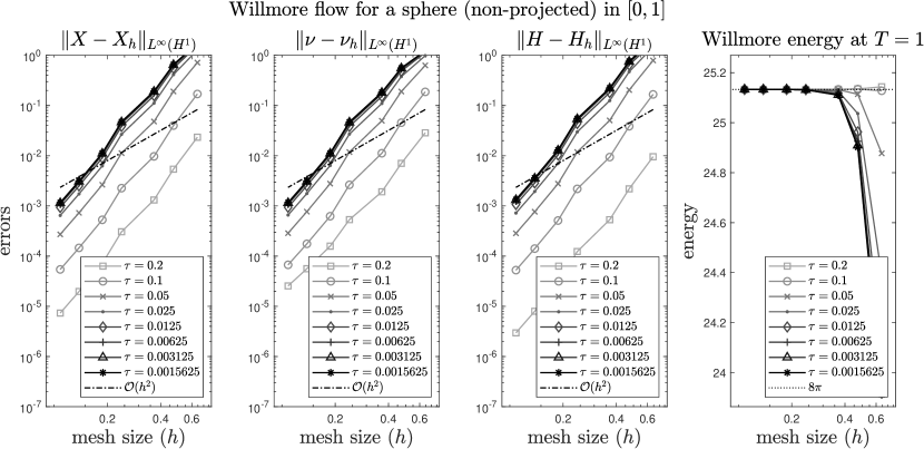
Figure 3: Spatial convergence of the BDF2 / quadratic ESFEM discretization (without projecting $nu_{h}$ and $z_{h}$) for the Willmore flow of a sphere for $T=1$.

In order to preserve important properties of the functions in the approximation, it is recommended to project the computed surface normal $\nu_{h}\approx\nu$ onto the unit sphere and the function $z_{h}\approx\nabla_{\Gamma}H$ onto the tangent space. This is done after every time step. The advantages of a normalising projection for $\nu_{h}$ were already explored in numerical experiments for mean curvature flow in KLL (19).

Figure 4 reports on the effect of the projections using a sphere of radius $1$: the left plots show the minimum ($\circ$) and maximum ($*$) lengths of the normal vectors, the middle plots the roundness of the surface (minimum ($\circ$) and maximum ($*$) distance from origin), and the right plots show the Willmore energy along the flows.

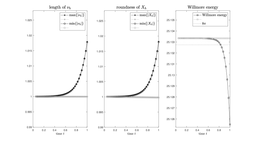
Figure 4: Comparing the effect of projecting $\nu_{h}$ and $z_{h}$ onto the unit sphere and the tangent plane, respectively, (black without projections, grey with projections) using a sphere (dof $=1914$, $\tau=0.025$) reporting on length of normal $\nu_{h}$, surface roundness (i.e. radius), and Willmore energy along the flow in $[0,1]$.

Figure 5 and 6 report on the same experiments for the algorithm with projections for the sphere and the Clifford torus, respectively. For the Clifford torus we used the linearly implicit Euler method (BDF1), whose damping property proved to be advantageous for this delicate experiment.

In Figures 3, 5 and 6 the spatial discretization error dominates, matching (exceeding even) the $O(h^{2})$ order of convergence (note the reference lines), in agreement with our theoretical results in Theorem 4.1.

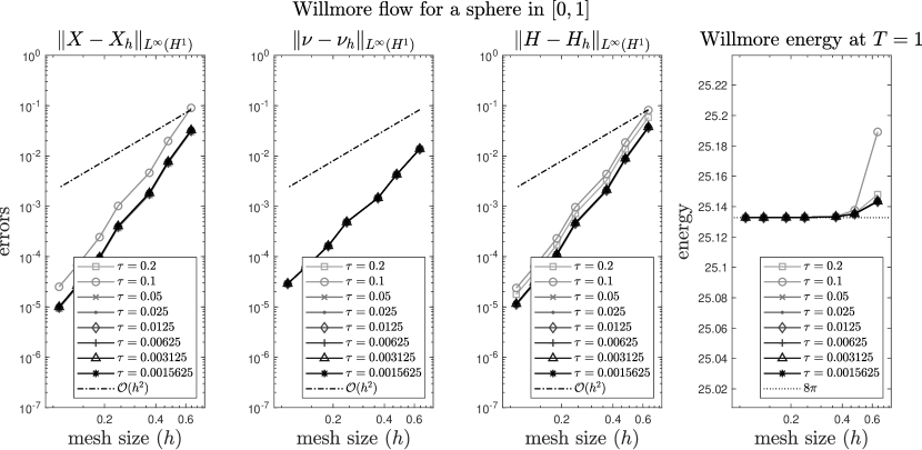
Figure 5: Spatial convergence of the BDF2 / quadratic ESFEM discretization (with projection of $\nu_{h}$ and $z_{h}$ onto the unit sphere and the tangent plane, respectively) for the Willmore flow of a sphere.

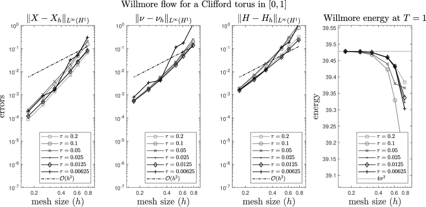
Figure 6: Spatial convergence of the BDF1 / quadratic ESFEM discretization (with projection of $\nu_{h}$ and $z_{h}$ onto the unit sphere and the tangent plane, respectively) for the Willmore flow of a Clifford torus.

7.2 Willmore flow towards stationary solutions

In Figure 7 we report on experiments for the surface evolution and Willmore energy for three surfaces: an ellipsoid, a surface of the shape of a red blood cell (cf. Dzi (08) and BGN (08)), and a periodically perturbed torus (cf. Dzi (08)). The meshes have $4978$, $8978$, and $12000$ nodes, respectively, and were integrated in $[0,4]$ with a time step size $\tau=0.2\cdot 2^{-8}\approx 7.8\cdot 10^{-4}$. In the last two rows, times $t=3$ and $4$, it can be observed that the algorithm leaves the surface stationary.

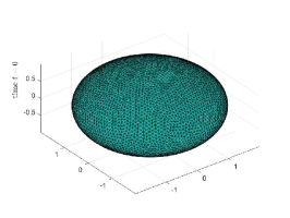
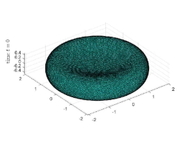
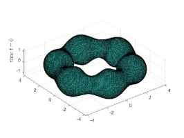
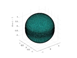
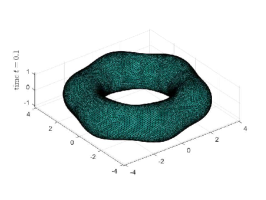
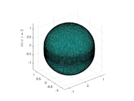
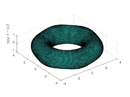
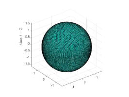
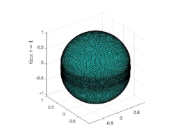
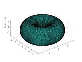
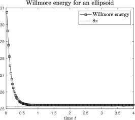
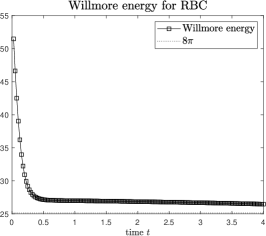
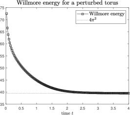
Figure 7: Surface evolutions at different times and corresponding Willmore energy

Appendix: Proof of Lemma 2

We came up with two independent proofs of Lemma 2, one based on local coordinates and the other one based on the formalism of Dziuk and Elliott in DE13a . As should be, both approaches yield the same result as stated in Lemma 2. Here we present the more straightforward proof based on DE13a .

The following commutator formula for tangential differential operators ($D_{i}=(\nabla_{\Gamma})_{i}$) is shown in (DE13a, , Lemma 2.6):

$$D_{i}D_{j}u-D_{j}D_{i}u=A_{jk}D_{k}u\nu_{i}-A_{ik}D_{k}u\nu_{j}\qquad(i,j=1,2,3),$$ (78)

where we use the convention to sum over repeated indices. We also recall that $A_{ij}=\ D_{i}\nu_{j}=A_{ji}$ and $H={\rm tr}(\nabla_{\Gamma}\nu)=D_{i}\nu_{i}$.

Using (78) we obtain (cf. the proof of Lemma 3.2 in DE13a )

$$D_{i}D_{i}D_{j}u= \ D_{i}\big{(}D_{j}D_{i}u+A_{jk}D_{k}u\nu_{i}-A_{ik}D_{k}u\nu_{j}\big{)}$$

$$= \ D_{i}D_{j}D_{i}u+D_{i}\big{(}D_{k}u(A_{jk}\nu_{i}-A_{ik}\nu_{j})\big{)}$$

$$= \ D_{i}D_{j}D_{i}u+D_{i}D_{k}u\big{(}A_{jk}\nu_{i}-A_{ik}\nu_{j}\big{)}$$

$$\ \phantom{D_{i}D_{j}D_{i}u}+D_{k}uD_{i}\big{(}A_{jk}\nu_{i}-A_{ik}\nu_{j}\big{)}.$$

The second term is then rewritten as

$$D_{i}D_{k}u\big{(}A_{jk}\nu_{i}-A_{ik}\nu_{j}\big{)}=\ A_{jk}D_{i}D_{k}u\nu_{i}-A_{ik}D_{i}D_{k}u\nu_{j}$$

$$= \ A_{jk}\big{(}D_{k}D_{i}u+A_{kl}D_{l}u\nu_{i}-A_{il}D_{l}u\nu_{k}\big{)}\nu_{i}-A_{ik}D_{i}D_{k}u\nu_{j}$$

$$= \ A_{jk}(D_{k}D_{i}u\nu_{i})+A_{jk}A_{kl}D_{l}u\nu_{i}\nu_{i}-A_{jk}A_{il}D_{l}u\nu_{k}\nu_{i}-A_{ik}D_{i}D_{k}u\nu_{j}$$

$$= \ -A_{jk}A_{ki}D_{i}u+A_{jk}A_{kl}D_{l}u-A_{jk}A_{il}D_{l}u\nu_{k}\nu_{i}-A_{ik}D_{i}D_{k}u\nu_{j}$$

$$= \ -(A^{2})_{ji}D_{i}u+(A^{2})_{jl}D_{l}u-A_{jk}A_{il}D_{l}u\nu_{k}\nu_{i}-A_{ik}D_{i}D_{k}u\nu_{j}$$

$$= \ -A_{jk}A_{il}D_{l}u\nu_{k}\nu_{i}-A_{ik}D_{i}D_{k}u\nu_{j}$$

$$= \ -A_{ik}D_{i}D_{k}u\nu_{j}.$$

In particular for the last term we have:

$$D_{i}\big{(}A_{jk}\nu_{i}-A_{ik}\nu_{j}\big{)}= \ D_{i}A_{jk}\nu_{i}-D_{i}A_{ik}\nu_{j}+A_{jk}D_{i}\nu_{i}-A_{ik}D_{i}\nu_{j}$$

$$= \ D_{i}A_{jk}\nu_{i}-D_{i}A_{ik}\nu_{j}+A_{jk}H-A_{ki}A_{ij}$$

$$= \ -\Delta_{\Gamma}\nu_{k}\nu_{j}\color[rgb]{0,0,0}+(HA-A^{2})_{jk}.$$

The third-order term is again rewritten using (78) as

$$D_{i}D_{j}D_{i}u= \ D_{j}D_{i}D_{i}u+A_{jk}D_{k}D_{i}u\nu_{i}-A_{ik}D_{k}D_{i}u\nu_{j},$$

which is further rewritten using

$$D_{k}D_{i}u\nu_{i}= \ D_{k}(D_{i}u\nu_{i})-D_{k}\nu_{i}D_{i}u=-A_{ki}D_{i}u,$$

$$D_{k}D_{i}u\nu_{j}= \ D_{k}(D_{i}u\nu_{j})-D_{k}\nu_{j}D_{i}u.$$

Therefore,

$$D_{i}D_{j}D_{i}u= \ D_{j}D_{i}D_{i}u-A_{jk}A_{ki}D_{i}u-A_{ik}D_{k}D_{i}u\nu_{j}$$

$$= \ D_{j}D_{i}D_{i}u-(A^{2})_{ji}D_{i}u-A_{ik}D_{k}D_{i}u\nu_{j}.$$

Altogether, the above calculations yield

$$D_{i}D_{i}D_{j}u$$

$$=D_{j}D_{i}D_{i}u-(A^{2})_{ji}D_{i}u-2A_{ik}D_{k}D_{i}u\nu_{j}-\Delta_{\Gamma}\nu_{k}\nu_{j}D_{k}u+(HA-A^{2})_{jk}D_{k}u$$

$$=D_{j}D_{i}D_{i}u-(A^{2})_{ji}D_{i}u-2D_{k}(A_{ik}D_{i}u)\nu_{j}+2D_{k}A_{ik}D_{i}u\nu_{j}$$

$$\quad-\Delta_{\Gamma}\nu_{k}\nu_{j}D_{k}u+(HA-A^{2})_{jk}D_{k}u$$

$$=D_{j}D_{i}D_{i}u-(A^{2})_{ji}D_{i}u-2D_{k}(A_{ik}D_{i}u)\nu_{j}+\Delta_{\Gamma}\nu_{k}\nu_{j}D_{k}u+(HA-A^{2})_{jk}D_{k}u.$$

This implies

$$\Delta_{\Gamma}\nabla_{\Gamma}u= \ \nabla_{\Gamma}\Delta_{\Gamma}u-A^{2}\nabla_{\Gamma}u-2\nabla_{\Gamma}\cdot(A\nabla_{\Gamma}u)\nu$$

$$\quad+(\Delta_{\Gamma}\nu\cdot\nabla_{\Gamma}u)\nu+(HA-A^{2})\nabla_{\Gamma}u,$$

which is the same as (8). ∎

References

- Bar [13] S. Bartels. A simple scheme for the approximation of the elastic flow of inextensible curves. IMA J. Numer. Anal., 33(4):1115–1125, 2013.
- [2] J.W. Barrett, H. Garcke, and R. Nürnberg. A parametric finite element method for fourth order geometric evolution equations. J. Comput. Phys., 222(1):441–467, 2007.
- [3] J.W. Barrett, H. Garcke, and R. Nürnberg. On the variational approximation of combined second and fourth order geometric evolution equations. SIAM J. Sci. Comput., 29(3):1006–1041, 2007.
- BGN [08] J.W. Barrett, H. Garcke, and R. Nürnberg. Parametric approximation of Willmore flow and related geometric evolution equations. SIAM J. on Sci. Comput., 31(1):225–253, 2008.
- BGN [15] J.W. Barrett, H. Garcke, and R. Nürnberg. Numerical computations of the dynamics of fluidic membranes and vesicles. Phys. Rev. E, 92(5):052704, 2015.
- BGN [19] J.W. Barrett, H. Garcke, and R. Nürnberg. Parametric finite element approximations of curvature driven interface evolutions. arXiv:1903.09462v1, 2019.
- BJSW [17] W. Bao, W. Jiang, D. J. Srolovitz, and Y. Wang. Stable equilibria of anisotropic particles on substrates: a generalized Winterbottom construction. SIAM J. Appl. Math., 77(6):2093–2118, 2017.
- BJWZ [17] W. Bao, W. Jiang, Y. Wang, and Q. Zhao. A parametric finite element method for solid-state dewetting problems with anisotropic surface energies. J. Comput. Phys., 330:380–400, 2017.
- Bla [29] W. Blaschke. Vorlesungen über Differentialgeometrie III. Grundlehren der mathematischen Wissenschaften. Springer-Verlag, Berlin, 1929.
- BMN [04] E. Bänsch, P. Morin, and R. H. Nochetto. Surface diffusion of graphs: variational formulation, error analysis, and simulation. SIAM J. Numer. Anal., 42(2):773–799, 2004.
- BMN [05] E. Bänsch, P. Morin, and R. H. Nochetto. A finite element method for surface diffusion: the parametric case. J. Comput. Phys., 203(1):321–343, 2005.
- BNP [10] A. Bonito, R. H. Nochetto, and M. S. Pauletti. Parametric FEM for geometric biomembranes. J. Comput. Phys., 229(9):3171–3188, 2010.
- CENC [96] J.W. Cahn, C.M. Elliott, and A. Novick-Cohen. The Cahn-Hilliard equation with a concentration dependent mobility: motion by minus the Laplacian of the mean curvature. European J. Appl. Math., 7(3):287–301, 1996.
- CLS+ [18] Y. Chen, J. Lowengrub, J. Shen, C. Wang, and S. Wise. Efficient energy stable schemes for isotropic and strongly anisotropic Cahn–Hilliard systems with the Willmore regularization. J. Comput. Phys., 365:56–73, 2018.
- DD [06] K. Deckelnick and G. Dziuk. Error analysis of a finite element method for the Willmore flow of graphs. Interfaces Free Bound., 8(1):21–46, 2006.
- DD [09] K. Deckelnick and G. Dziuk. Error analysis for the elastic flow of parametrized curves. Math. Comp., 78(266):645–671, 2009.
- DDE [03] K. Deckelnick, G. Dziuk, and C.M. Elliott. Error analysis of a semidiscrete numerical scheme for diffusion in axially symmetric surfaces. SIAM J. Numer. Anal., 41(6):2161–2179, 2003.
- [18] K. Deckelnick, G. Dziuk, and C. M. Elliott. Computation of geometric partial differential equations and mean curvature flow. Acta Numerica, 14:139–232, 2005.
- [19] K. Deckelnick, G. Dziuk, and C.M. Elliott. Fully discrete finite element approximation for anisotropic surface diffusion of graphs. SIAM J. Numer. Anal., 43(3):1112–1138, 2005.
- DE [07] G. Dziuk and C.M. Elliott. Finite elements on evolving surfaces. IMA J. Numer. Anal., 27(2):262–292, 2007.
- [21] G. Dziuk and C.M. Elliott. Finite element methods for surface PDEs. Acta Numerica, 22:289–396, 2013.
- [22] G. Dziuk and C.M. Elliott. –estimates for the evolving surface finite element method. Math. Comp., 82(281):1–24, 2013.
- Dem [09] A. Demlow. Higher–order finite element methods and pointwise error estimates for elliptic problems on surfaces. SIAM J. Numer. Anal., 47(2):805–807, 2009.
- DKS [15] K. Deckelnick, J. Katz, and F. Schieweck. A -finite element method for the Willmore flow of two-dimensional graphs. Math. Comp., 84(296):2617–2643, 2015.
- DLM [12] G. Dziuk, C. Lubich, and D.E. Mansour. Runge–Kutta time discretization of parabolic differential equations on evolving surfaces. IMA J. Numer. Anal., 32(2):394–416, 2012.
- Dzi [88] G. Dziuk. Finite elements for the Beltrami operator on arbitrary surfaces. Partial differential equations and calculus of variations, Lecture Notes in Math., 1357, Springer, Berlin, pages 142–155, 1988.
- Dzi [08] G. Dziuk. Computational parametric Willmore flow. Numer. Math., 111(1):55–80, 2008.
- Eck [12] K. Ecker. Regularity theory for mean curvature flow. Birkhäuser, Boston, 2012.
- ES [10] C.M. Elliott and B. Stinner. Modeling and computation of two phase geometric biomembranes using surface finite elements. J. Comput. Phys., 229(18):6585–6612, 2010.
- Hel [73] W. Helfrich. Elastic properties of lipid bilayers: theory and possible experiments. Zeitschrift für Naturforschung C, 28(11-12):693–703, 1973.
- Hui [84] G. Huisken. Flow by mean curvature of convex surfaces into spheres. J. Differential Geometry, 20(1):237–266, 1984.
- KLL [19] B. Kovács, B. Li, and C. Lubich. A convergent evolving finite element algorithm for mean curvature flow of closed surfaces. Numer. Math., 143(4):797–853, 2019.
- KLLP [17] B. Kovács, B. Li, C. Lubich, and C.A. Power Guerra. Convergence of finite elements on an evolving surface driven by diffusion on the surface. Numer. Math., 137(3):643–689, 2017.
- Kov [18] B. Kovács. High-order evolving surface finite element method for parabolic problems on evolving surfaces. IMA J. Numer. Anal., 38(1):430–459, 2018.
- KS [01] E. Kuwert and R. Schätzle. The Willmore flow with small initial energy. J. Differential Geom., 57(3):409–441, 2001.
- KS [02] E. Kuwert and R. Schätzle. Gradient flow for the Willmore functional. Comm. Anal. Geom., 10(2):307–339, 2002.
- LM [15] C. Lubich and D.E. Mansour. Variational discretization of wave equations on evolving surfaces. Math. Comp., 84(292):513–542, 2015.
- Man [12] C. Mantegazza. Lecture Notes on Mean Curvature Flow. Progress in Mathematics, Volume 290. Birkhäuser, Corrected Printing 2012.
- MN [14] F. C. Marques and A. Neves. Min-Max theory and the Willmore conjecture. Annals Math., 179(2):683–782, 2014.
- Mul [57] W. W. Mullins. Theory of thermal grooving. J. Appl. Phys., 28:333–339, 1957.
- Poz [15] P. Pozzi. Computational anisotropic Willmore flow. Interfaces Free Bound., 17(2):189–232, 2015.
- PS [04] P.-O. Persson and G. Strang. A simple mesh generator in MATLAB. SIAM Review, 46(2):329–345, 2004.
- PS [18] P. Pozzi and B. Stinner. Elastic flow interacting with a lateral diffusion process: the one-dimensional graph case. IMA J. Numer. Anal., 39(1):201–234, 03 2018.
- Rus [05] R.E. Rusu. An algorithm for the elastic flow of surfaces. Interfaces and Free Boundaries, 7(3):229–239, 2005.
- Tho [24] G. Thomsen. Grundlagen der konformen flächentheorie. Abh. Math. Seminar Univ. Hamburg, 3(1):31–56, 1924.
- Wal [15] S.W. Walker. The Shape of Things: a Practical Guide to Differential Geometry and the Shape Derivative. SIAM, Philadelphia, 2015.
- Wil [65] T.J. Willmore. Note on embedded surfaces. An. Sti. Univ.“Al. I. Cuza” Iasi Sect. I a Mat.(NS) B, 11:493–496, 1965.
- Wil [93] T. J. Willmore. Riemannian Geometry. Oxford Science Publications. The Clarendon Press, Oxford University Press, New York, 1993.
- ZJB [20] Q. Zhao, W. Jiang, and W. Bao. A parametric finite element method for solid-state dewetting problems in three dimensions. SIAM J. Sci. Comput., 42(1):B327–B352, 2020.