Correctness by construction
for probabilistic programs

Abstract

The “correct by construction” paradigm is an important component of modern Formal Methods, and here we use the probabilistic Guarded-Command Language pGCL to illustrate its application to probabilistic programming.

pGCL extends Dijkstra’s guarded-command language GCL with probabilistic choice, and is equipped with a correctness-preserving refinement relation $(\ref{)}$ that enables compact, abstract specifications of probabilistic properties to be transformed gradually to concrete, executable code by applying mathematical insights in a systematic and layered way.

Characteristically for “correctness by construction”, as far as possible the reasoning in each refinement-step layer does not depend on earlier layers, and does not affect later ones.

We demonstrate the technique by deriving a fair-coin implementation of any given discrete probability distribution. In the special case of simulating a fair die, our correct-by-construction algorithm turns out to be “within spitting distance” of Knuth and Yao’s optimal solution.

1 Testing probabilistic programs?

Edsger Dijkstra argued [1, p3] that the construction of correct programs requires mathematical proof, since “…program testing can be used very effectively to show the presence of bugs but never to show their absence.” But for programs that are constructed to exhibit some form of randomisation, regular testing can’t even establish that presence: odd program traces are almost always bound to turn up even in correctly operating probabilistic systems.

Thus evidence of quantitative errors in probabilistic systems would require many, many traces to be subjected to detailed statistical analysis — yet even then debugging probabilistic programs remains a challenge when that evidence has been assembled. Unlike standard (non-probabilistic programs), where a failed test can often pinpoint the source of the offending error in the code, it’s not easy to figure out what to change in the implementation of probabilistic programs in order to move closer towards “correctness” rather than further away.

Without that unambiguous relationship between failed tests and the coding errors that cause them, Dijkstra’s caution regarding proofs of programs is even more apposite. In this paper we describe such a proof method for probability: correctness-by-construction. In a sentence, to apply “CbC” one constructs the program and its proof at the same time, letting the requirement that there be a proof guide the design decisions taken while constructing the program.

Like standard programs, probabilistic programs incorporate mathematical insights into algorithms, and a correctness-by-construction method should allow a program developer to refer rigorously to those insights by applying development steps that preserve “probabilistic correctness”. Probabilistic correctness is however notoriously unintuitive. For example, the solution of the infamous Monty Hall problem caused such a ruckus in the mathematical community that even Paul Erdös questioned the correct analysis [14].  Yet once coded up as a program [10, p22], the Monty Hall problem is only four lines long! More generally though, many widely relied-upon programs in security are quite short, and yet still pose significant challenges for correctness.

We describe correctness-by-construction in the context of pGCL, a small programming language which restores demonic choice to Kozen’s landmark (purely) probabilistic semantics [7, 8] while using the syntax of Dijkstra’s GCL [2]. Its basic principles are that correctness for programs can be described by a generalisation of Hoare logic that includes quantitative analysis; and it has a definition of refinement that allows programs to be developed in such a way that both functional and probabilistic properties are preserved.

2 Enabling Correctness by Construction — pGCL

The setting for correctness-by-construction of probabilistic programs is provided by pGCL –the probabilistic Guarded-Command Language– which contains both abstraction and (stepwise) refinement [10]. We begin by reviewing its origins, then its treatment of probabilistic choice and demonic choice, and finally its realisation of CbC.

(This section can be skimmed on first reading: just collect pGCL syntax from Figs. 2–4, and then skip directly to Sec. 3.)

As we will not be treating non-terminating programs, we can base our description here on quite simple models for sequential (non-reactive) programs. The state space is some set $S$ and, in its simplest terms, a program takes an initial state to a final state: it (its semantics) therefore has type $S\,{\rightarrow}\,S$.

The three subsections that follow describe logics based on successive enrichments of this, the simplest model, and even the youngest of those logics is by now almost 25 years old: thus we will be “reviewing” rather than inventing.

The first enrichment, Sec. 2.1, is based on the model $S\,{\rightarrow}\,{\mathbb{P}}S$ that allows demonic nondeterminism,  so facilitating abstraction; then in Sec. 2.2 the model $S\,{\rightarrow}\,\mathbb{D}S$ replaces demonic nondeterminism by probabilistic choice, losing abstraction (temporarily) but in its place gaining the ability to describe probabilistic outcomes; and finally in Sec. 2.3 the model $S\,{\rightarrow}\,{\mathbb{P}}\mathbb{D}S$ restores demonic nondeterminism, allowing programs that can abstract from precise probabilities. Using syntax we will make more precise in those sections, simple examples of the three increments in expressivity are

1. x:= H    Set variable x to H (as in any sequential language);

2. x:$\in$ {H,T}    Set x’s value demonically from the set $\{\texttt{H},\texttt{T}\}$;

3. x:$\in$ H $\mathbin{{}_{{\nicefrac{{2}}{{3}}}}\kern-0.50003pt\oplus}$ T    Set x’s value from the set $\{\texttt{H},\texttt{T}\}$ with probability $\nicefrac{{2}}{{3}}$ for H and $\nicefrac{{1}}{{3}}$ for T, a “biased coin”; and

4. x:$\in$ H $\mathbin{{}_{{\nicefrac{{1}}{{3}}}}\kern-0.50003pt\oplus_{{\nicefrac{{1}}{{3}}}}}$ T    Set x from the set $\{\texttt{H},\texttt{T}\}$ with probability at least $\nicefrac{{1}}{{3}}$ each way, a “capricious coin”.

The last example of those (4) is the most general: for (3) is x:$\in$ H $\mathbin{{}_{{\nicefrac{{2}}{{3}}}}\kern-0.50003pt\oplus_{{\nicefrac{{1}}{{3}}}}}$ T; and (2) is x:$\in$ H $\mathbin{{}_{{0}}\kern-0.50003pt\oplus_{{0}}}$ T; and finally (1) is x:$\in$ H $\mathbin{{}_{{1}}\kern-0.50003pt\oplus_{{0}}}$ T.

2.1 Floyd/Hoare/Dijkstra: pre- and postconditions: (1,2) above

We assume a typical sequential programming language with variables, expressions over those variables, assignment (of expressions to variables), sequential composition (semicolon or line break), conditionals and loops. It is more or less Dijkstra’s guarded command language [2], and is based on the model $S\,{\rightarrow}\,{\mathbb{P}}S$, where ${\mathbb{P}}S$ is the set of all subsets of $S$.

The weakest precondition of program Prog in such a language, with respect to a postcondition post given as a first-order formula over the program variables, is written wp(Prog,post) and means

the weakest formula (again on the program variables) that must hold before Prog executes in order to ensure that post holds after Prog executes [2].

In a typical compositional style, the wp of a whole program is determined by the wp of its components.

At left is a “generic” Floyd annotation of a flowchart containing only one program element. If the annotation pre holds “on the way in” to the program Prog, then annotation post will hold on the way out. At right is an example with specific annotations and a specific program.

In the Hoare style the right-hand example would be written

$$\{{\tt x}=1\}~{}~{}\texttt{x:= x+1}~{}~{}\{{\tt x}=2\}\makebox[0.0pt][l]{{\quad.}}$$

In the Dijsktra style it would be written $\texttt{x=1}\mathbin{\Rightarrow}\texttt{{wp}({x:= x+1},~{}x=2)}$.

They all three have the same meaning.

Figure 1: Floyd-style annotated flowchart

We group Dijkstra, Hoare and Floyd together because the Dijkstra-style implication $~{}{\texttt{{pre}}}\mathbin{\Rightarrow}\textsf{wp}(\texttt{{{{Prog}}}},{\texttt{{post}}})~{}$ has the same meaning as the Hoare-style triple $~{}\{{\texttt{{pre}}}\}~{}{\texttt{{Prog}}}~{}\{{\texttt{{post}}}\}~{}$ which in turn has the same meaning as the original Floyd-style flowchart annotation, as shown in Fig. 1 [3, 4]. All three mean “If pre holds of the state before execution of Prog, then post will hold afterwards.”

Finally, a notable –but incidental– feature of Dijkstra’s approach was that (demonic) nondeterminism arose naturally, as an abstraction from possible concrete implementations.  That is why we use $S\,{\rightarrow}\,{\mathbb{P}}S$ rather than $S\,{\rightarrow}\,S$ here. In later work (by others) that abstraction was made more explicit by including explicit syntax for a binary “demonic choice” between program fragments, a composition Left $\mathbin{\sqcap}$ Right that could behave either as the program Left or as the program Right. But that operator ($\mathbin{\sqcap}$) was not really an extension of Dijkstra’s work, because his (more verbose) conditional

IF True $$\rightarrow \rightarrow$$ Left   – If True holds, then this branch may be taken.   True Right  – If True holds, then also this branch may be taken. FI – (Dijkstra terminated all IF’s with FI’s.)

was there in his original guarded-command language, introducing demonic choice naturally as an artefact of the program-design process — and it expressed exactly the same thing. The ($\mathbin{\sqcap}$) merely made it explicit.

2.2 Kozen: probabilistic program logic: (3) above

Kozen extended Dijkstra-style semantics to probabilistic programs, again over a sequential programming language but now based on the model $S\,{\rightarrow}\,\mathbb{D}S$, where $\mathbb{D}S$ is set of all discrete distributions in $S$.  He replaced Dijkstra’s demonic nondeterminism ($\mathbin{\sqcap}$) by a “probabilistic nondeterminism” operator ($\mathbin{{}_{{p}}\kern-0.50003pt\oplus}$) between programs, understood so that  Left $\mathbin{{}_{{p}}\kern-0.50003pt\oplus}$ Right  means “Execute Left with probability $p$ and Right with probability $1{-}p$.” The probability $p$ is (very) often $\nicefrac{{1}}{{2}}$ so that  coin:= Heads $\mathbin{{}_{{\nicefrac{{1}}{{2}}}}\kern-0.50003pt\oplus}$ coin:= Tails  means “Flip a fair coin.” But probability p can more generally be any real number, and more generally still it can even be an expression in the program variables.

Kozen’s corresponding extension of Floyd/Hoare/Dijkstra [7, 8] replaced Dijkstra’s logical formulae with real-valued expressions (still over the program variables); we give examples below. The “original” Dijkstra-style formulae remain as a special case where real number 1 represents $\mathit{True}$  and 0 represents $\mathit{False}$; and Dijkstra’s definitions of wp simply carry through essentially as they are… except that an extra definition is necessary, for the new construct ($\mathbin{{}_{{{\texttt{{p}}}}}\kern-0.50003pt\oplus}$), where Kozen defines that

$$\textsf{wp}(\texttt{{{{Left}}}\;$\mathbin{{}_{{{\texttt{{p}}}}}\kern-0.50003pt\oplus}$\;{{{Right}}}},{\texttt{{post}}})$$

is $${\texttt{{p}}}\cdot\textsf{wp}(\texttt{{{{Left}}}},{\texttt{{post}}})~{}+~{}(1{-}{\texttt{{p}}})\cdot\textsf{wp}(\texttt{{{{Right}}}},{\texttt{{post}}})\makebox[0.0pt][l]{{\quad.}}$$

With this single elegant extension, it turns out that in general wp(Prog,post) is the expected value, given as a (real valued) expression over the initial state, of what post will be in the final state, i.e. after Prog has finished executing from that initial state. (The initial/final emphasis simply reminds us that it is the same as for Dijkstra: the weakest precondition is what must be true in the initial state for the postcondition to be true in the final state.) For example we have that

$$\textsf{wp}(\texttt{x:= 1-y\,$\mathbin{{}_{{\nicefrac{{1}}{{3}}}}\kern-0.50003pt\oplus}$\;x:= 3*x},~{}~{}~{}\texttt{x}+3)~{}~{}~{}~{}~{}~{}\textrm{is}~{}~{}~{}~{}~{}~{}\nicefrac{{1}}{{3}}(1{-}\texttt{y}+3)~{}+~{}\nicefrac{{2}}{{3}}(3\texttt{x}{+}3)\quad,$$

that is the real-valued expression $3\frac{1}{3}+2\texttt{x}-\texttt{y}/3$ in which both x and y refer to their values in the initial state.

More impressive though is that if we introduce the convention that brackets $[-]$ convert Booleans to numbers, i.e. that $[\mathit{True}]=1$ and $[\mathit{False}]=0$, we have in general for Boolean-valued prop the convenient idiom

$$\textsf{wp}(\texttt{{{{Prog}}}},[\,{\texttt{{prop}}}])$$ (1)

is $$\textrm{``the probability that {{{Prog}}}\ establishes property {{{prop}}}''},\,$$

And if –further– it happens that the “probabilistic” program Prog actually contains no probabilistic choices at all, then (1) just above has value 1 just when Prog is guaranteed to establish post, and is 0 otherwise: it is in that sense that the Dijkstra-style semantics “carries through” into the Kozen extension. That is, if Prog contains no probabilistic choice, and post is a conventional (Boolean valued) formula, then we have

Dijkstra style $$[\,\textsf{wp}(\texttt{{{{Prog}}}},{\texttt{{post}}})\,]$$

is the same as Kozen style $$\textsf{wp}(\texttt{{{{Prog}}}},[\,{\texttt{{post}}}\,])\makebox[0.0pt][l]{.\,}$$

The full power of the Kozen approach, however, starts to appear in examples like this one below: we flip two fair coins and ask for the probability that they show the same face afterwards. Using the (Dijkstra) weakest-precondition rule that wp(Prog1;Prog2, post) is simply wp(Prog1, wp(Prog2,post)),  we can calculate

	$\begin{array}[t]{@{}llll}\textsf{wp}(\texttt{{\tt c1:= H $\mathbin{{}_{{\nicefrac{{1}}{{2}}}}\kern-0.50003pt\oplus}$\, c1:= T;~{}c2:= H $\mathbin{{}_{{\nicefrac{{1}}{{2}}}}\kern-0.50003pt\oplus}$\, c2:= T}},~{}~{}~{}[\texttt{c1}=\texttt{c2}])\end{array}$
=	$\begin{array}[t]{@{}llll}\textsf{wp}(\texttt{{\tt c1:= H $\mathbin{{}_{{\nicefrac{{1}}{{2}}}}\kern-0.50003pt\oplus}$\, c1:= T}},~{}~{}~{}\textsf{wp}(\texttt{{\tt c2:= H $\mathbin{{}_{{\nicefrac{{1}}{{2}}}}\kern-0.50003pt\oplus}$\, c2:= T}},[\texttt{c1}=\texttt{c2}]))\end{array}$
=	$\begin{array}[t]{@{}llll}\textsf{wp}(\texttt{{\tt c1:= H $\mathbin{{}_{{\nicefrac{{1}}{{2}}}}\kern-0.50003pt\oplus}$\, c1:= T}},~{}~{}~{}\nicefrac{{1}}{{2}}[\texttt{c1}=\texttt{H}]+(1{-}\nicefrac{{1}}{{2}})[\texttt{c1}=\texttt{T}])\end{array}$
=	$\begin{array}[t]{@{}llll}\nicefrac{{1}}{{2}}(\nicefrac{{1}}{{2}}[\texttt{H}=\texttt{H}]+\nicefrac{{1}}{{2}}[H=\texttt{T}])+\nicefrac{{1}}{{2}}(\nicefrac{{1}}{{2}}[\texttt{T}=\texttt{H}]+\nicefrac{{1}}{{2}}[\texttt{T}=\texttt{T}])\end{array}$
=	$\begin{array}[t]{@{}llll}\nicefrac{{1}}{{2}}(\nicefrac{{1}}{{2}}\cdot 1+\nicefrac{{1}}{{2}}\cdot 0)+\nicefrac{{1}}{{2}}(\nicefrac{{1}}{{2}}\cdot 0+\nicefrac{{1}}{{2}}\cdot 1)\end{array}$
=	$\begin{array}[t]{@{}llll}\nicefrac{{1}}{{4}}+\nicefrac{{1}}{{4}}\end{array}$
=	$\begin{array}[t]{@{}llll}\nicefrac{{1}}{{2}}\textrm{~{},\quad that is that the probability that $\texttt{c1}\,{=}\,\texttt{c2}$ is $\nicefrac{{1}}{{2}}$.}\end{array}$

A nice further exercise for seeing this probabilistic wp at work is to repeat the above calculation when one of the coins uses ($\mathbin{{}_{{{\texttt{{p}}}}}\kern-0.50003pt\oplus}$) but ($\mathbin{{}_{{\nicefrac{{1}}{{2}}}}\kern-0.50003pt\oplus}$) is retained for the other, confirming that the answer is still $\nicefrac{{1}}{{2}}$.

name	syntax	semantics
expectation post	real-valued expression over the program variables	(the usual)
expression E	expression over the program variables (of any type)	(the usual)
condition C	Boolean-valued expression over the program variables	(the usual)
substitution	E1[x$\backslash$E2]	Replace all free occurrences of x in E1 by E2 (with the usual caveats.)
assignment	x:= E	Evaluate E; assign it to x.
		wp(x:= E, post) = post[x$\backslash$E]
sequential composition	Prog1;Prog2	Execute Prog1 then Prog2.
	wp(Prog1;Prog2, post) = wp(Prog1, wp(Prog2,post))
conditional	IF C THEN Prog1 ELSE Prog2	Evaluate Boolean C, then execute Prog1 or Prog2 accordingly.
	wp(IF C THEN Prog1 ELSE Prog2, post)
	= $[{\texttt{{C}}}]{\cdot}\textsf{wp}(\texttt{{{{Prog1}}}},{\texttt{{post}}})+[\neg{\texttt{{C}}}]{\cdot}\textsf{wp}(\texttt{{{{Prog2}}}},{\texttt{{post}}})$
loop	WHILE C DO Prog	Evaluate Boolean C, then execute Prog (and repeat), or exit, accordingly.
The usual least fixed point, based on
$\texttt{WHILE {{{C}}}~{}DO {{{Prog}}}}\quad=\quad\texttt{IF {{{C}}}~{}THEN ({{{Prog}}};~{}WHILE {{{C}}}~{}DO {{{Prog}}})}$

The above cases cover the constructs of pGCL without probabilistic- or demonic choice, but nevertheless defined with Kozen-style “numeric” wp’s which, applied to “post-expectations” give “pre-expectations”.

Figure 2: Syntax and wp-semantics for “restricted” pGCL

2.3 McIver/Morgan: pre- and post-expectations

Following Kozen’s probabilistic semantics at Sec. 2.2 just above (which itself turned out later to be a special case of Jones and Plotkin’s probabilistic powerdomain contruction [5]) we restored demonic choice to the programming language and called it pGCL [12, 10]. It contains both demonic ($\mathbin{\sqcap}$) and probabilistic ($\mathbin{{}_{{{\texttt{{p}}}}}\kern-0.50003pt\oplus}$) choices; its model is $S\,{\rightarrow}\,{\mathbb{P}}\mathbb{D}S$; and it is the language we will use for the correct-by-construction program development we carry out below [10]. Figures 2–4 summarise its syntax and its wp-logic.

To illustrate demonic- vs. probabilistic choice, we’ll revisit the two-coin program from above. This time, one coin will have a probability-$p$ bias for some constant $0\,{\leq}\,p\,{\leq}\,1$ (thus acting as a fair coin just when $p$ is $\nicefrac{{1}}{{2}}$). The other choice will be purely demonic.

name	syntax	semantics
probabilistic choice	Prog1 $\mathbin{{}_{{{\texttt{{p}}}}}\kern-0.45003pt\oplus}$ Prog2	Evaluate p, which must be in $[0,1]$, then execute Prog1 with that probability; otherwise execute Prog2.
wp(Prog1$\mathbin{{}_{{{\texttt{{p}}}}}\kern-0.45003pt\oplus}$ Prog2, post)  $=$  p$\cdot$wp(Prog1​, post)+(1-p)$\cdot$wp(Prog2​, post)
demonic choice	Prog1$\;\mathbin{\sqcap}$ Prog2	Choose demonically whether to execute Prog1 or Prog2.
wp(Prog1 $\mathbin{\sqcap}$ Prog2, post)  $=$  wp(Prog1​, post) $\mathbin{\sf min}$ wp(Prog2​, post)

These “extra” cases cover the probabilistic- and demonic choice constructs of pGCL.

Figure 3: Syntax and wp-semantics for pGCL’s choice constructs

name	syntax	semantics
do nothing	SKIP	wp(SKIP, post) = post .
fail	ABORT	wp(ABORT, post) = 0 .
probabilistic assignment	x:$\in$ E1$\mathbin{{}_{{{\texttt{{p}}}}}\kern-0.45003pt\oplus}$ E2	As for (x:= E1) $\mathbin{{}_{{{\texttt{{p}}}}}\kern-0.45003pt\oplus}$ (x:= E2) .
demonic assignment	x:$\in$ E1 $\mathbin{\sqcap}$ E2	As for (x:= E1) $\mathbin{\sqcap}$ (x:= E2) .
probabilistic	IF p THEN Prog1	As for Prog1 $\mathbin{{}_{{{\texttt{{p}}}}}\kern-0.45003pt\oplus}$ Prog2 .
conditional	ELSE Prog2
probabilistic	WHILE p DO Prog	As for ordinary loop,
loop		but using probabilistic conditional.

The cases above introduce special commands, abbreviations and “syntactic sugar” for pGCL.

Command SKIP allows an “ELSE-less” conditional, as used e.g. in Fig. 2, to be defined in the usual way, as IF C THEN Prog1 ELSE SKIP.

Command ABORT allows wp(WHILE C DO Prog, post), as a least fixed point, to be defined as the supremum of

wp(ABORT, post)

wp(IF C THEN (Prog;ABORT), post)

wp(IF C THEN (Prog;(IF C THEN (Prog;ABORT))), post)

$\vdots$ ,

which exists (in spite of the reals’ being unbounded) because it can be shown by structural induction that

$$\textsf{wp}(\texttt{{{{Prog}}}},{\texttt{{post}}})~{}~{}~{}\leq~{}~{}~{}{\texttt{{post}}}\textrm{\quad,}$$

and that wp(Prog,$-$) is continuous, for all programs Prog. The above is therefore a chain, is dominated by post itself, and attains the limit at $\omega$.

Figure 4: Syntax and wp-semantics for pGCL’s choice constructs

We start with the (two-statement) program

c1:= H $$\mathbin{{}_{{p}}\kern-0.50003pt\oplus} \mathbin{\sqcap}$$  c1:= H c2:= H     c2:= T  ,

where the first statement is probabilistic and the second is demonic, and ask, as earlier, “What is the probability that the two coins end up equal?” We calculate

	$\begin{array}[t]{@{}llll}\textsf{wp}(\texttt{{\tt c1:= H $\mathbin{{}_{{p}}\kern-0.50003pt\oplus}$\, c1:= T;~{}c2:= H {$\mathbin{\sqcap}$}\;c2:= T}},~{}~{}~{}[\texttt{c1}=\texttt{c2}])\end{array}$
=	$\begin{array}[t]{@{}llll}\textsf{wp}(\texttt{{\tt c1:= H $\mathbin{{}_{{p}}\kern-0.50003pt\oplus}$\, c1:= T}},~{}~{}~{}\textsf{wp}(\texttt{{\tt c2:= H {$\mathbin{\sqcap}$}\;c2:= T}},~{}[\texttt{c1}=\texttt{c2}]))\end{array}$
=	$\begin{array}[t]{@{}llll}\textsf{wp}(\texttt{{\tt c1:= H $\mathbin{{}_{{p}}\kern-0.50003pt\oplus}$\, c1:= T}},~{}~{}~{}[\texttt{c1}=\texttt{H}]~{}\mathbin{\sf min}~{}[\texttt{c1}=\texttt{T}])\end{array}$
=	$\begin{array}[t]{@{}llll}p\,{\cdot}([\texttt{H}=\texttt{H}]~{}\mathbin{\sf min}~{}[\texttt{H}=\texttt{T}])+(1{-}{\it p}){\cdot}([\texttt{T}=\texttt{H}]~{}\mathbin{\sf min}~{}[\texttt{T}=\texttt{T}])\end{array}$
=	$\begin{array}[t]{@{}llll}p\,{\cdot}(1~{}\mathbin{\sf min}~{}0)+(1{-}p){\cdot}(0~{}\mathbin{\sf min}~{}1)\end{array}$
=	$\begin{array}[t]{@{}llll}p\,{\cdot}0+(1{-}p){\cdot}0\end{array}$
=	$\begin{array}[t]{@{}llll}0\quad,\end{array}$

to reach the conclusion that the probability of the two coins’ being equal finally… is zero. And that highlights the way demonic choice is usually treated: it’s a worst-case outcome. The “demon” –thought of as an agent– always tries to make the outcome as bad as possible: here because our desired outcome is that the coins be equal, the demon always sets the coin c2 so they will differ. If we repeated the above calculation with postcondition $\texttt{c1}{\neq}\texttt{c2}$ instead, the result would again be zero: if we change our minds, want the coins to differ, then the demon will change his mind too, and act to make them the same. 

Implicit in the above treatment is that the c2 demon knows the outcome of the c1 flip — which is reasonable because that flip has already happened by the time it’s the demon’s turn.

Now we reverse the statements, so that the demon goes first: it must set c2 without knowing beforehand what c1 will be. The program becomes

c2:= H   $$\mathbin{\sqcap} \mathbin{{}_{{p}}\kern-0.50003pt\oplus}$$  c2:= T c1:= H   c1:= T  ,

and we calculate

	$\begin{array}[t]{@{}llll}\textsf{wp}(\texttt{{\tt c2:= H \,$\mathbin{\sqcap}$\;c2:= T;~{}c1:= H $\mathbin{{}_{{\it p}}\kern-0.50003pt\oplus}$\, c1:= T}},~{}~{}~{}[\texttt{c1}=\texttt{c2}])\end{array}$
=	$\begin{array}[t]{@{}llll}\textsf{wp}(\texttt{{\tt c2:= H \,$\mathbin{\sqcap}$\;c2:= T}},~{}~{}~{}\textsf{wp}(\texttt{{\tt c1:= H $\mathbin{{}_{{\it p}}\kern-0.50003pt\oplus}$\, c1:= T}},~{}[\texttt{c1}=\texttt{c2}]))\end{array}$
=	$\begin{array}[t]{@{}llll}\textsf{wp}(\texttt{{\tt c2:= H \,$\mathbin{\sqcap}$\;c2:= T}},~{}~{}~{}p\,{\cdot}[\texttt{H}=\texttt{c2}]+(1{-}p){\cdot}[\texttt{T}=\texttt{c2}])\end{array}$
=	$\begin{array}[t]{@{}llll}p\,{\cdot}[\texttt{H}=\texttt{H}]+(1{-}p){\cdot}[\texttt{T}=\texttt{H}]~{}~{}\mathbin{\sf min}~{}~{}p\,{\cdot}[\texttt{H}=\texttt{T}]+(1{-}p){\cdot}[\texttt{T}=\texttt{T}]\end{array}$
=	$\begin{array}[t]{@{}llll}p\,{\cdot}1+(1{-}p){\cdot}0~{}~{}\mathbin{\sf min}~{}~{}p\,{\cdot}0+(1{-}p){\cdot}1\end{array}$
=	$\begin{array}[t]{@{}llll}p~{}\mathbin{\sf min}~{}(1{-}p)\makebox[0.0pt][l]{{\quad.}}\end{array}$

Since the demon set flip c2 without knowing what the c1-flip would be (because it had not happened yet), the worst it can do is to choose c2 to be the value that it is known c1 is least likely to be — which is just the result above, the lesser of $p$ and $1{-}p$. If –as before– we change our minds and decide instead that we would like the coins to be different, then the demon adapts by choosing c2 to be the value that c1 is most likely to be.

Either way, the probability our postcondition will be achieved, the pre-expectation of its characteristic function, is the same $p\,\mathbin{\sf min}\,(1{-}p)$ — so that only when $p\,{=}\,\nicefrac{{1}}{{2}}$, i.e. when $p\,{=}\,(1{-}p)$, does the demon gain no advantage.

3 Probabilistic correctness by construction in action 

Our first example problem conceptually will be to achieve a binary choice of arbitrary bias using only a fair coin. With the apparatus of Sec. 2.3 however, we can immediately move from conception to precision:

We must write a pGCL program that implements  Left $\mathbin{{}_{{p}}\kern-0.50003pt\oplus}$ Right ,under the constraint that the only probabilistic choice operator we are allowed to use in the final (pGCL) program is $(\mathbin{{}_{{\nicefrac{{1}}{{2}}}}\kern-0.50003pt\oplus})$.

This is not a hard problem mathematically: the probabilistic calculation that solves it is elementary. Our point here is to use this simple problem to show how such solutions can be calculated within a programming-language context, while maintaining rigour (possibly machine-checkable) at every step.

The final program is given at (8) in Sec. 3.5.

3.1 Step 1 — a simplification

We’ll start by simplifying the problem slightly, instantiating the programs Left and Right to x:= 1 and x:= 0 respectively. Our goal is thus to implement

x:$$\in \mathbin{{}_{{p}}\kern-0.50003pt\oplus}$$ 1  0 , (2)

for arbitrary $p$, and our first step is to create two other distributions $1\,{\mathbin{{}_{{q}}\kern-0.50003pt\oplus}}\,0$ and $1\,{\mathbin{{}_{{r}}\kern-0.50003pt\oplus}}\,0$ whose average is $1\,{\mathbin{{}_{{p}}\kern-0.50003pt\oplus}}\,0$ — that is

$$\nicefrac{{1}}{{2}}\times(\,(1\,{\mathbin{{}_{{q}}\kern-0.50003pt\oplus}}\,0)+(1\,{\mathbin{{}_{{r}}\kern-0.50003pt\oplus}}\,0)\,)~{}~{}~{}=~{}~{}~{}(1\,{\mathbin{{}_{{p}}\kern-0.50003pt\oplus}}\,0)\makebox[0.0pt][l]{{\quad.}}$$ (3)

A fair coin will then decide whether to carry on with $1\,\mathbin{{}_{{q}}\kern-0.50003pt\oplus}\,0$ or with $1\,\mathbin{{}_{{r}}\kern-0.50003pt\oplus}\,0$.

Trivially (3) holds just when $(q{+}r)/2=p$, and if we represent $p,q,r$ as variables in our program, we can achieve (3) by the double assignment

IF p $$\leq \nicefrac{{1}}{{2}} \rightarrow \geq \nicefrac{{1}}{{2}} \rightarrow \color[rgb]{0,0,1}\left\{\,{\tt{p=(q+r)/2}}\,\right\}$$   q,r:= 0,2p   p    q,r:= 2p-1,1   FI  , (4)

whose postcondition indicates what the assignment has established. If we follow that with a fair-coin flip between continuing with q or with r, viz.

IF p $$\leq \nicefrac{{1}}{{2}} \rightarrow \geq \nicefrac{{1}}{{2}} \rightarrow \in \mathbin{{}_{{\tt q}}\kern-0.50003pt\oplus} \mathbin{{}_{{\nicefrac{{1}}{{2}}}}\kern-0.50003pt\oplus} \in \mathbin{{}_{{\tt r}}\kern-0.50003pt\oplus} (\mathbin{{}_{{\nicefrac{{1}}{{2}}}}\kern-0.40002pt\oplus})$$   q,r:= 0,2p – Here q is 0.   p    q,r:= 2p-1,1 – Here r is 1. FI (x: 1  0)  (x: 1  0) – The fair coin here is permitted. (5)

then we should have implemented Program (2). But what have we gained?

The gain is that, whichever branch of the conditional is taken, there is a $\nicefrac{{1}}{{2}}$ probability that the problem we have yet to solve will be either $(\mathbin{{}_{{0}}\kern-0.50003pt\oplus})$ or $(\mathbin{{}_{{1}}\kern-0.50003pt\oplus})$, both of which are trivial. If we were unlucky, well… then we just try again. But how do we show rigorously that Program (2) and Program (5) are equal?

If we look back at Program (4), we find the assertion $\color[rgb]{0,0,1}\left\{\,{\tt{p=(q+r)/2}}\,\right\}$ which is easy to establish by conventional Hoare-logic or Dijkstra-wp reasoning from the conditional just before it. (We removed it from Program (5) just to reduce clutter.) Rigour is achieved by calculating

	$\begin{array}[t]{@{}llll}\textsf{wp}(\texttt{(x:\kern-1.00006pt$\in$\kern-1.99997pt\ 1\;$\mathbin{{}_{{\tt q}}\kern-0.50003pt\oplus}$\;0)~{}$\mathbin{{}_{{\nicefrac{{1}}{{2}}}}\kern-0.50003pt\oplus}$~{}(x:\kern-1.00006pt$\in$\kern-1.99997pt\ 1\;$\mathbin{{}_{{\tt r}}\kern-0.50003pt\oplus}$\;0)},~{}~{}~{}{\texttt{{post}}})\end{array}$
$=$	$\begin{array}[t]{@{}llll}\nicefrac{{1}}{{2}}\;\textsf{wp}(\texttt{(x:\kern-1.00006pt$\in$\kern-1.99997pt\ 1\;$\mathbin{{}_{{\tt q}}\kern-0.50003pt\oplus}$\;0)},{\texttt{{post}}})~{}+~{}\nicefrac{{1}}{{2}}\;\textsf{wp}(\texttt{(x:\kern-1.00006pt$\in$\kern-1.99997pt\ 1\;$\mathbin{{}_{{\tt r}}\kern-0.50003pt\oplus}$\;0)},{\texttt{{post}}})\end{array}$
$=$	$\begin{array}[t]{@{}llll}\nicefrac{{\tt q}}{{2}}\cdot{\texttt{{post}}}[\texttt{x}\backslash 1]+\nicefrac{{(1-\texttt{q})}}{{2}}\cdot{\texttt{{post}}}[\texttt{x}\backslash 0]+\nicefrac{{\tt r}}{{2}}\cdot{\texttt{{post}}}[\texttt{x}\backslash 1]+\nicefrac{{(1-\texttt{r})}}{{2}}\cdot{\texttt{{post}}}[\texttt{x}\backslash 0]\end{array}$
$=$	$\begin{array}[t]{@{}llll}(\texttt{q}{+}\texttt{r})/2\cdot{\texttt{{post}}}[\texttt{x}\backslash 1]~{}+~{}(1-(\texttt{q}{+}\texttt{r})/2)\cdot{\texttt{{post}}}[\texttt{x}\backslash 0]\end{array}$
$=$	$\begin{array}[t]{@{}llll}\texttt{p}\cdot{\texttt{{post}}}[\texttt{x}\backslash 1]~{}+~{}(1{-}\texttt{p})\cdot{\texttt{{post}}}[\texttt{x}\backslash 0]\end{array}$ “$\color[rgb]{0,0,1}\left\{\,{\tt{p=(q+r)/2}}\,\right\}$”
$=$	$\begin{array}[t]{@{}llll}\textsf{wp}(\texttt{x:\kern-1.00006pt$\in$\kern-1.99997pt\ 1\;$\mathbin{{}_{{\tt p}}\kern-0.50003pt\oplus}$\;0},~{}~{}~{}{\texttt{{post}}})\makebox[0.0pt][l]{{\quad,}}\end{array}$

for arbitrary postcondition post where at the end we used $\color[rgb]{0,0,1}\left\{\,{\tt{p=(q+r)/2}}\,\right\}$. Thus $(\ref{p1643})\,{=}\,(\ref{p1714})$ because for any post their pre-expectations agree.

3.2 Step 2 — intuition suggests a loop

We now return to the remark “… then we just try again.” If we replace the final fair-coin flip  (x:$\in$ 1 $\mathbin{{}_{{\tt q}}\kern-0.50003pt\oplus}$ 0) $\mathbin{{}_{{\nicefrac{{1}}{{2}}}}\kern-0.50003pt\oplus}$ (x:$\in$ 1 $\mathbin{{}_{{\tt r}}\kern-0.50003pt\oplus}$ 0)  by  p:$\in$ q $\mathbin{{}_{{\nicefrac{{1}}{{2}}}}\kern-0.50003pt\oplus}$ r  then –intuitively– we are in a position to “try again” with  x:$\in$ 1 $\mathbin{{}_{{p}}\kern-0.50003pt\oplus}$ 0 . Although it is the same as the statement we started with, we have made progress because variable p has been updated — and with probability $\nicefrac{{1}}{{2}}$ it is either 0 or 1 and we are done. If it is not, then we arrange for a second execution of

IF p $$\leq \nicefrac{{1}}{{2}} \rightarrow \geq \nicefrac{{1}}{{2}} \rightarrow \in \mathbin{{}_{{\nicefrac{{1}}{{2}}}}\kern-0.50003pt\oplus}$$   q,r:= 0,2p   p    q,r:= 2p-1,1 FI p: q  r (6)

and, if still p is neither 0 nor 1, then … we need a loop.

3.3 Step 3 — introduce a loop

We have already shown that

$$Program\,(\ref{p1643})~{}~{}~{}=~{}~{}~{}Program\,(\ref{p1852});~{}Program\,(\ref{p1643})\makebox[0.0pt][l]{{\quad.}}$$

A general equality for sequential programs (including probabilistic) tells us that in that case also we have

$$Program\,(\ref{p1643})~{}~{}~{}=~{}~{}~{}\texttt{WHILE {{{C}}}\ DO $Program\,(\ref{p1852})$ OD; $Program\,(\ref{p1643})$}\makebox[0.0pt][l]{\quad}$$

for any loop condition C, provided the loop terminates. Intuitively that is clear because, if Program (2) can annihilate Program (6) once from the right, then it can do so any number of times. A rigorous argument appeals to the fixed-point definition of WHILE, which is where termination is used. (If C were False, so that the loop did not terminate, the rhs would be Abort, thus providing a clear counter-example.)

For probabilistic loops, the usual “certain” termination is replaced with almost-sure termination, abbreviated AST, which means that the loop terminates with probability one: put the other way, that would be that the probability of iterating forever is zero. For example the program

c:= H; WHILE c=H DO c:$$\in \mathbin{{}_{{\nicefrac{{1}}{{2}}}}\kern-0.50003pt\oplus}$$ H  T OD .

terminates almost surely because the probability of flipping T forever is zero.

A reasonably good AST rule for probabilistic loops is that the variant is (as usual) a natural number, but must be bounded above; and instead of having to decrease on every iteration, it is sufficient to have a non-zero probability of doing so [13, 10].  The variant for our example loop just above is [c=H], which has probability $\nicefrac{{1}}{{2}}$ of decreasing from [H=H], that is 1, to [T=H] on each iteration.

The loop condition C for our program will be $0\,{<}\,\texttt{p}\,{<}\,1$ and the variant comes directly from there: it is [0$<$p$<$1], which has probability of $\nicefrac{{1}}{{2}}$ of decreasing from 1 to 0 on each iteration: and when it is 0, that is $0\,{<}\,\texttt{p}\,{<}\,1$ is false, the loop must exit. With that, we have established that our original Program (2) equals the looping program

WHILE 0 < p < 1 DO IF p $$\leq \nicefrac{{1}}{{2}} \rightarrow \geq \nicefrac{{1}}{{2}} \rightarrow \in \mathbin{{}_{{\nicefrac{{1}}{{2}}}}\kern-0.50003pt\oplus} \color[rgb]{0,0,1}\left\{\,{\tt{\texttt{p}=1\lor\texttt{p}=0}}\,\right\} \in \mathbin{{}_{{\texttt{p}}}\kern-0.50003pt\oplus}$$   q,r:= 0,2p   p    q,r:= 2p-1,1 FI p: q  r OD x: 1  0 ,

where the assertion at the loop’s end is the negation of the loop guard.

3.4 Step 4 — use the loop’s postcondition

There is still the final x:$\in$ 1 $\mathbin{{}_{{\texttt{p}}}\kern-0.50003pt\oplus}$ 0 to be dealt with, at the end; but the assertion $\color[rgb]{0,0,1}\left\{\,{\tt{\texttt{p}=1\lor\texttt{p}=0}}\,\right\}$ just before it means that it executes only when p is zero or one. So it can be replaced by IF p=0 THEN x:$\in$ 1$\mathbin{{}_{{1}}\kern-0.50003pt\oplus}$0 ELSE x:$\in$ 1$\mathbin{{}_{{0}}\kern-0.50003pt\oplus}$0 , i.e. with just  x:= p . Mathematically, that would be checked by showing for all post-expectations post that

$$\texttt{p}=1\lor\texttt{p}=0~{}~{}~{}\mathbin{\Rightarrow}~{}~{}~{}\textsf{wp}(\texttt{x:\kern-1.00006pt$\in$\kern-1.99997pt\ 1\,{$\mathbin{{}_{{\texttt{p}}}\kern-0.50003pt\oplus}$}\,0},{\texttt{{post}}})=\textsf{wp}(\texttt{x:= p},{\texttt{{post}}})\makebox[0.0pt][l]{{\quad.}}$$

But it’s a simple-enough step just to believe (unless you were using mechanical assistance, in which case it would be checked).

And so now the program is complete: we have implemented  x:$\in$ 1$\mathbin{{}_{{p}}\kern-0.50003pt\oplus}$0  by a step-by-step correctness-by-construction process that delivers the program

WHILE 0 < p < 1 DO IF p $$\leq \nicefrac{{1}}{{2}} \rightarrow \geq \nicefrac{{1}}{{2}} \rightarrow \in \mathbin{{}_{{\nicefrac{{1}}{{2}}}}\kern-0.50003pt\oplus}$$   q,r:= 0,2p   p    q,r:= 2p-1,1 FI p: q  r OD x:= p (7)

in which only fair choices appear. And each step is provably correct.

3.5 Step 5 — after-the-fact optimisation

There is still one more thing that can (provably) be done with this program, and it’s typical of this process: only when the pieces are finally brought together do you notice a further opportunity. It makes little difference — but it is irresistible.

Before carrying it out, however, we should be reminded of the way in which these five steps are isolated from each other, how all the layers are independent. This is an essential part of CbC, that the reasoning can be carried out in small, localised areas, and that it does not matter –for correctness– where the reasoning’s target came from; nor does it matter where it is going.

Thus even if we had absolutely no idea what Program (7) was supposed to be doing, still we would be able to see that if we are replacing x by p at the end, we could just as easily replace it at the beginning; and then we can remove the variable p altogether. That gives

– Now $$p p \leq \nicefrac{{1}}{{2}} \rightarrow \texttt{x}\,{=}\,\nicefrac{{1}}{{2}} \geq \nicefrac{{1}}{{2}} \rightarrow \in \mathbin{{}_{{\nicefrac{{1}}{{2}}}}\kern-0.50003pt\oplus} \in \mathbin{{}_{{p}}\kern-0.40002pt\oplus} 0\,{\leq}\,p\,{\leq}\,1$$ is again a parameter, as it was in the original specification. x:= WHILE 0 < x < 1 DO IF x    q,r:= 0,2x – When , these two   x    q,r:= 2x-1,1 – branches have the same effect. FI x: q  r OD , – The above implements  x: 10  for any . (8)

and we are done. When $p$ is 0 or 1, it takes no flips at all; when $p$ is $\nicefrac{{1}}{{2}}$, it takes exactly one flip; and for all other values the expected number of flips is 2.

We notice that Program (8) appears to contain demonic choice, in that when $\texttt{x}\,{=}\,\nicefrac{{1}}{{2}}$ the conditional could take either branch. The nondeterminism is real — even though the effect is the same in either case, that  q,r:= 0,1  occurs. But genuinely different computations are carried out to get there: in the first branch $2(\nicefrac{{1}}{{2}})\,-\,1$ is evaluated to 0; and in the second branch $2(\nicefrac{{1}}{{2}})$ is evaluated to 1.

This is not an accident: we recall from Sec. 2.1 that for Dijkstra such nondeterminism arises naturally as part of the program-construction process. Where did it come from in this case?

The specification from which this conditional IF $\cdots$ FI arose was set out much earlier, at (3) which given $p$ has many possible solutions in $q,r$. One of them for example is $q\,{=}\,r\,{=}\,p$ which however would have later given a loop whose non-termination would prevent Step 3 at Sec. 3.3. With an eye on loop termination, therefore, we took a design decision that at least one of $q,r$ should be “extreme”, that is 0 or 1. To end up with $q\,{=}\,0$, what is the largest that $p$ could be without sending $r$ out of range, that is strictly more than 1? It’s $p\,{=}\,\nicefrac{{1}}{{2}}$, and so the first IF-condition is $p\,{\leq}\,\nicefrac{{1}}{{2}}$. The other condition $p\,{\geq}\,\nicefrac{{1}}{{2}}$ arises similarly, and it absolutely does not matter that they overlap: the program will be correct whichever IF-branch taken in that case.

And, in the end –in (8) just above– we see that indeed that is so.

4 Implementing any discrete choice with a fair coin

Suppose instead of trying to implement a biased coin (as we have been doing so far), we want to implement a general (discrete) probabilistic choice of x’s value from its type, say a finite set $\cal X$, but still using only a fair coin in the implementation. An example would be choosing x uniformly from $\{x_{0},x_{1},x_{2}\}$, i.e. a three-way fair choice. But what we develop below will work for any discrete distribution on a finite set $\cal X$ of values: it does not have to be uniform.

The combination of probability and abstraction allows a development like the one in Sec. 3 just above to be replayed, but a greater level of generality. We begin with a variable d of type $\mathbb{D}{\cal X}$,  where we recall that $\cal X$ is the type of x; and our specification is  x:$\in$ d , that is “Set x according to distribution d.”

name	syntax	semantics
choose from set	x:$\in$ set
wp(x:$\in$ set, post) = ($\mathbin{\sf min}$ $e\,{\mid}\,e\,{\in}\,{\texttt{{set}}}$ . post[x$\backslash$$e$])
assign “such that”	x:$|$ property(x)
wp(x:$|$ property(x), post) = ($\mathbin{\sf min}$ $e\,{\mid}$ property($e$) . post[x$\backslash$$e$])

The above generalise to more than a single variable, and are consistent with the earlier definitions: thus

	$\begin{array}[t]{@{}llll}~{}\texttt{x:= a\;\,$\mathbin{\sqcap}$\,\;x:= b}{}\end{array}$
$=$	$\begin{array}[t]{@{}llll}~{}\texttt{x:\kern-0.90005pt$\in$\kern-1.79997pt\ \{a,b\}}{}\end{array}$
$=$	$\begin{array}[t]{@{}llll}~{}\texttt{x:\kern-0.90005pt$|$\kern-1.79997pt\ x$\,\in\,$\{a,b\}}~{}\makebox[0.0pt][l]{{\quad.}}\end{array}$

By analogy with “choose from set” (but not itself an abstraction) we have also

name	syntax	semantics
choose from distribution	x:$\in$ dist
wp(x:$\in$ dist, post) = ($\sum\,e\,{\mid}\,e\,{\in}\,\lceil{\texttt{{dist}}}\rceil$ . dist($e$)$\,\cdot\,$post[x$\backslash$$e$])    ,

where ${\texttt{{dist}}}(e)$ is the probability that dist assigns to $e$ and $\lceil{\texttt{{dist}}}\rceil$ is the support of dist, the set of elements to which it assigns non-zero probability. 

It is just the expected value of post, considered as a function of x, over the distribution dist on x. (Since  E1 $\mathbin{{}_{{p}}\kern-0.45003pt\oplus}$ E2  is a distribution, the definition above agrees with the earlier meaning of  x:$\in$ E1 $\mathbin{{}_{{p}}\kern-0.45003pt\oplus}$ E2  that we gave in Fig. 4 as an abbreviation.)

Figure 5: Abstraction in pGCL

4.1 Replaying earlier steps from Sec. 3

Our first step –Step 1– is to declare two more $\mathbb{D}{\cal X}$-typed variables d0 and d1, and –as in Sec. 3.1– specify that they must be chosen so that their average is the original distribution d; for that we use the pGCL nondeterministic-choice construct “assign such that” (with syntax borrowed from Dafny [9]), from Fig. 5, to write

d0,d1:$$| \texttt{d}=(\texttt{d0}{+}\texttt{d1})/2$$  – Choose d0,d1 so that their average is d. (9)

The analogy with our earlier development is that there the distribution d was specifically $1\,{\mathbin{{}_{{p}}\kern-0.50003pt\oplus}}\,0$, and we assigned

$$\begin{array}[]{p{6em}lcl@{~~}l}if $\texttt{p}\,{\leq}\nicefrac{{1}}{{2}}$&\texttt{d0},\texttt{d1}&=&(1\;\mathbin{{}_{{\tt 0}}\kern-0.50003pt\oplus}\;0),\hfil~{}~{}&(1\;\mathbin{{}_{{\tt 2\texttt{p}}}\kern-0.50003pt\oplus}\;0)\\ if $\texttt{p}\,{\geq}\nicefrac{{1}}{{2}}$&\texttt{d0},\texttt{d1}&=&(1\;\mathbin{{}_{{\tt 2\texttt{p}{-}1}}\kern-0.50003pt\oplus}\;0),\hfil~{}~{}&(1\;\mathbin{{}_{{\tt 1}}\kern-0.50003pt\oplus}\;0)\makebox[0.0pt][l]{{\quad,}}\end{array}$$

which is a refinement $(\ref{)}$ of (9).

Our second step is to re-establish the  x:$\in$ d  -annihilating property that

$$\texttt{Program\,(\ref{p1102}); d:\kern-1.00006pt$\in$\kern-1.99997pt\ d0\,{$\mathbin{{}_{{\nicefrac{{1}}{{2}}}}\kern-0.50003pt\oplus}$}\,d1; x:\kern-1.00006pt$\in$\kern-1.99997pt\ d}~{}~{}~{}=~{}~{}~{}\texttt{x:\kern-1.00006pt$\in$\kern-1.99997pt\ d}\makebox[0.0pt][l]{{\quad,}}$$ (10)

which is proved using wp-calculations agains a general post-expectation post, just as before: instead of the assertion $\color[rgb]{0,0,1}\left\{\,{\tt{\texttt{p}=(\texttt{q}+\texttt{r})/2}}\,\right\}$ used at the end of Step 1, we use the assertion $\color[rgb]{0,0,1}\left\{\,{\tt{\texttt{d}=(\texttt{d0}{+}\texttt{d1})/2}}\,\right\}$ established by the assign-such-that.

The third step is again to introduce a loop. But we recall from Step 3 earlier that the loop must be almost-surely terminating and, to show that, we need a variant function. Here we have no q,r that might be set to 0 or 1; we have instead d0,d1. Our variant will be that the “size” of one of these distributions must decrease strictly, where we define the size of a discrete distribution to be the number of elements to which it assigns non-zero probability.  But our specification  d0,d1:$|$ $\texttt{d}=(\texttt{d0}{+}\texttt{d1})/2$  above does not require that decrease; and so we must backtrack in our CbC and make sure that it does.

And we have made an important point: developments following CbC rarely proceed as they are finally presented: the dead-ends are cut off, and only the successful path is left for the audit trail. It highlights the multiple uses of CbC — that on the one hand, used for teaching, the dead-ends are shown in order to learn how to avoid them; used in production, the successful path remains so that it can be modified in the case that requirements change. 

Thus to establish AST of the loop –that it terminates with probability one– we strengthen the split of d achieved by  d0,d1:$|$ $(\texttt{d0}{+}\texttt{d1})/2=\texttt{d}$  with the decreasing-variant requirement, that either $|\texttt{d0}|\,{<}\,|\texttt{d}|$ or $|\texttt{d1}|\,{<}\,|\texttt{d}|$, where we are writing $|{-}|$ for “size of”. Then the variant $|\texttt{d}|$ is guaranteed strictly to decrease with probabililty $\nicefrac{{1}}{{2}}$ on each iteration. That is we now write

d0,d1:$$| (\texttt{d0}{+}\texttt{d1})/2=\texttt{d}\;\land\;(|\texttt{d0}|\,{<}\,|\texttt{d}|\lor|\texttt{d1}|\,{<}\,|\texttt{d}|)$$  , (11)

replacing (9), for the nondeterministic choice of d0 and d1. We do not have to re-prove its annihilation property, because the new statement (11) is a refinement of the (9) from before (It has a stronger postcondition.) and so preserves all its functional properties. In fact that is the definition of refinement.

Our next step is to reduce the nondeterminism in (11) somewhat, choosing a particular way of achieving it: to “split” d into two parts d0,d1 such that the size of at least one part is smaller, we choose two subsets $X_{0},X_{1}$ of $\cal X$ whose intersection contains at most one element. That is illustrated in Fig. 6, where $X_{0}=\{\textsf{A},\textsf{B},\textsf{C}\}$ and $X_{1}=\{\textsf{C},\textsf{D}\}$. Further, we require that the probabilities $\texttt{d}(X_{0})$ and $\texttt{d}(X_{1})$ assigned by d to $X_{0}{-}X_{1}$ and $X_{1}{-}X_{0}$ are both no more than $\nicefrac{{1}}{{2}}$.  Those constraints mean that we can always arrange the subsets so that the “$\nicefrac{{1}}{{2}}$-line” of Fig. 6 either goes strictly through $X_{0}\,{\cap}\,X_{1}$ (if they overlap) or runs between them (if they do not).

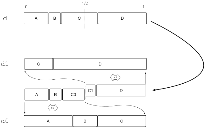
Suppose that $\cal X$ is $\{\textsf{A},\textsf{B},\textsf{C},\textsf{D}\}$, and that the distribution d in $\cal X$ that we start with is indicated by the size of the rectangles: the size $|\tt{d}|$ of d here is therefore 4, because it contains 4 rectangles. We choose $X_{0}$ to be $\{\textsf{A},\textsf{B},\textsf{C}\}$ and $X_{1}$ to be $\{\textsf{C},\textsf{D}\}$, so that $X_{0}{-}X_{1}$ is $\{\textsf{A},\textsf{B}\}$ and $X_{1}{-}X_{0}$ is $\{\textsf{D}\}$, and both $\texttt{d}(X_{0}{-}X_{1})$ and $\texttt{d}(X_{1}{-}X_{0})$ are no more than $\nicefrac{{1}}{{2}}$. Their overlap is $\{\textsf{C}\}$, whose probability the “$\nicefrac{{1}}{{2}}$-line” splits into two pieces: one piece joins d0 and the other piece joins d1.

Thus by dividing the overall rectangle (representing $\cal X$ itself) exactly in the middle, at least one side  must contain strictly fewer than $|\tt{d}|$ rectangles — and if we double the size of each small rectangle, we get our two distributions d1 and d2 such that $\texttt{d}=(\texttt{d0}+\texttt{d1})/2$ and either $|\texttt{d0}|\,{<}\,|\texttt{d}|$ or $|\texttt{d1}|\,{<}\,|\texttt{d}|$.

Figure 6: Dividing a discrete distribution into two pieces

We then construct d0 by restricting d to just $X_{0}$, then doubling all the probabilities in that restriction; if they sum to more than 1, we then trim any excess from the one element in $X_{0}\,{\cap}\,X_{1}$ that $X_{0}$ shares with $X_{1}$. The analogous procedure is applied to generate d1. In Fig. 6 for example we chose sizes $0.2$, $0.1$, $0.3$ and $0.4$ for the four regions, and the $\nicefrac{{1}}{{2}}$ line went through the third one. On the left, the $0.2$ and $0.1$ and $0.3$ are doubled to $0.4$ and $0.2$ and $0.6$, summing to $1.2$; thus $0.2$ is trimmed from the $0.6$, leaving $0.4$ assigned to C. The analogous procedure applies on the right.

4.2 “Decomposition of data into data structures”

The quote is from Wirth [15]. Our program is currently

WHILE |d|$$\neq | (\texttt{d0}{+}\texttt{d1})/2=\texttt{d}\;\land\;(|\texttt{d0}|\,{<}\,|\texttt{d}|\lor|\texttt{d1}|\,{<}\,|\texttt{d}|) \in \mathbin{{}_{{\nicefrac{{1}}{{2}}}}\kern-0.50003pt\oplus} \in =$$1 DO d0,d1:  d: d0  d1 OD x: d // This is aa trivial choice, because |d|1 here. (12)

And it is correct: it does refine x:$\in$ d — but it is rather abstract. Our next development step will be to make it concrete by realising the distribution-typed variables and the subsets of $\cal X$ as “ordinary” datatypes using scalars and lists. In correctness-by-construction this is done by deciding, before that translation process begins, what the realisations will be — and only then is the abstract program transformed, piece by piece. The relation between the abstract- and concrete types is called a coupling invariant.

Although an obvious approach is to order the type $\cal X$, say as $x_{1},x_{2},\ldots,x_{N}$ and then to realise discrete distributions as lists of length $N$ of probabilities (summing to 1), a more concise representation is suggested by the fact that for example we represent a two-point distribution $x_{1}\mathbin{{}_{{p}}\kern-0.50003pt\oplus}x_{2}$ as just one number $p$, with the $1{-}p$ implied. Thus we will represent the distribution $p_{1},p_{2},\ldots\,p_{N}$ as the list of length $N{-}1$ of “accumulated” probabilities: in this case for $p$ we would have a list

$$p_{1},~{}~{}p_{1}{+}p_{2},~{}~{}\ldots,~{}~{}\sum_{n=1}^{N-1}p_{n}\makebox[0.0pt][l]{{\quad,}}$$

leaving off the $N^{th}$ element of the list since it would always be 1 anyway. Subsets of $\cal X$ will be pairs low,high of indices, meaning $\{x_{\tt low},\ldots,x_{\tt high}\}$, and although that can’t represent all subsets of $\cal X$, contiguous subsets are all we will need. Carrying out that transformation gives following concrete version of our abstract program Program (12) below, where the abstract d is represented as the concrete dL[low:high] , which is the coupling invariant.

– Discrete distribution d in $$\cal X N N {\cal X} \neq \texttt{low}\,{=}\,\texttt{high} \{x_{\tt low}\} \{x_{\texttt{low}},\ldots,x_{\texttt{high}}\} X_{0} x_{1},x_{2},\ldots \,\land\, X_{0} \{x_{\texttt{low0}},\ldots,x_{\texttt{high0}}\} X_{1} x_{N},x_{N-1},\ldots \leq \,\land\, X_{1} \{x_{\texttt{low1}},\ldots,x_{\texttt{high1}}\} \in \mathbin{{}_{{\nicefrac{{1}}{{2}}}}\kern-0.50003pt\oplus} x_{\texttt{low}}$$ of size is realised here as dL (for “d-list”). low,high:= 1, – Initial support is all of . WHILE low  high DO –  means support is – Current support is . – Find by examining the probabilities of n:= low – Determine dL0 as in lhs of Fig. 6. WHILE  n<highdL[n]<1/2  DO dL0[n]:= 2*dL[n]; n:= n+1 OD low0,high0:= low,n – Subset is  . – Find by examining the probabilities of n:= high-1 – Determine dL1 as in rhs of Fig. 6. WHILE  lown1/2<dL[n]  DO dL1[n]:= 2*dL[n]-1; n:= n-1 OD low1,high1:= n+1,high – Subset is  . – Use fair coin to choose between dL0 and dL1. (dL,low,high): (dL0,low0,high0)  (dL1,low1,high1) OD x:= – Extract sole element of point distribution’s support. (13)

Figure 7: Implement any discrete choice using only a fair coin.

And in Program (13) of Fig. 7 we have, finally, a concrete program that can actually be run. Notice that it has exactly the same structure as Program (12): split (the realisations of) d into d0 and d1; overwrite d with one of them; exit the loop when |d| is one.

Neverthess, as earlier in Sec. 3.5, further development steps might still be possible now that everything is together in one place:  and indeed, recognising that only one of dL0,dL1 will be used, we can rearrange Program (13)’s body so that only that only one of them will be calculated — and it can be updated as we go. That gives our really-final-this-time program (14) in Fig. 8, which will -without further intervention– use a fair coin to choose a value $x_{n}$ according to any given discrete distribution $d$ on finite $\cal X$. Its expected number of coin flips is no worse than $2N{-}2$, where $N$ is the size of $\cal X$, thus agreeing with expected 2 flips for the program (8) in Sec. 3.5 that dealt with the simpler case $d=(1\mathbin{{}_{{p}}\kern-0.50003pt\oplus}0)$ where $\cal X$ was $\{1,0\}$.

– Assume discrete distribution $$d {\cal X}=\{x_{1},\ldots,x_{N}\} N N {\cal X} \neq \texttt{low}\,{=}\,\texttt{high} \{x_{\tt low}\} \,\land\, \leq \,\land\, x_{\texttt{low}}$$ over of size – has been represented cumulatively in list dL, as described above. low,high:= 1, – Initial support is all of . WHILE low  high DO –  means support is – Fair coin flipped here. (Recall Fig. 4.) IF 1/2 THEN – Then update dL as in lhs of Fig. 6. n:= low WHILE  n<highdL[n]<1/2 DO dL[n]:= 2*dL[n]; n:= n+1 OD high:= n ELSE – Else update dL as in rhs of Fig. 6. n:= high-1 WHILE  lown1/2<dL[n]  DO dL[n]:= 2*dL[n]-1; n:= n-1 OD low:= n+1 FI OD x:= – Extract sole element of point distribution dL’s support. (14)

Figure 8: Optimisation of Program (13)

It’s again worth emphasising –because it is the main point– that the correctness arguments for all of these steps are isolated from each other: in CbC every step’s correctness is determined by looking at that step alone. Thus for example nothing in the translation process just above involved reasoning about the earlier steps, whether Program (12) actually implemented the  x:$\in$ d  that we started with: we didn’t care, and we didn’t check. We just translated Program (12) into Program (13) regardless. And the subsequent rearrangement of (13) into Program (14) similarly made no use of Program (13)’s provenence.

All that is to be contrasted with the more common approach in which only intuition (and experience, and skill) is used, in which our final Program (14) might be written all at once at this concrete level, only then checking (testing, debugging, hoping) afterwards that our intuitions were correct. A transliteration of Program (14) into Python is given in App. 0.A.

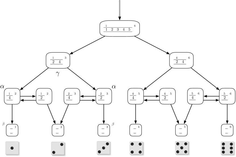
Each interior node has two possible successors chosen with equal probability, and each final-die node is reached with the same probability $\nicefrac{{1}}{{6}}$. There are 17 nodes, and the expected number of coin flips is 4.

The nodes’ origins are shown by labelling them with low, d and high from the states in the generating program that gave rise to them, representing the current probability distribution d yet to be realised over over the remaining subset $\{\texttt{low},\ldots,\texttt{high}\}$ of possible results. With probabilities normalised out of 6 for neatness, a typical label is

$$\begin{array}[]{llllll}{}^{\texttt{low}}&&&&&{}^{\texttt{high}}\\[-4.5pt] \cline{1-5}\cr\lx@intercol\hfil\longleftarrow 6{\times}\texttt{d}\longrightarrow\hfil\lx@intercol&\makebox[0.0pt][l]{{\quad,}}\\[-0.90005pt] \cline{1-5}\cr\end{array}$$

where we recall that d gives the sum of the probabilities for $x_{\tt{low}},x_{\tt{low}+1},\ldots,x_{\tt{high}-1}$ and that d for $x_{\texttt{high}}$ is left out, because it is always 1. Thus for example $\texttt{low}=2$ and $\texttt{high}=3$ and $\texttt{d}=[4]$ represents the distribution over support $\{2,3\}$ of $\nicefrac{{4}}{{6}}$ for 2 and $1{-}\nicefrac{{4}}{{6}}$ for 3, that is $2\mathbin{{}_{{\nicefrac{{2}}{{3}}}}\kern-0.45003pt\oplus}3$.

 

The well-known (optimal) algorithm of Knuth and Yao for simulating a die with a fair coin has 13 states and $\nicefrac{{11}}{{3}}$ expected coin flips [6] — and it can be obtained from here by one last correctness-preserving step. Eliminate the choice $\gamma$, so that the two $\alpha$ and the two $\beta$ nodes are merged; since that also merges the two die-rolls 1 and 3, restore the $\gamma$ choice as a new fair choice $\gamma^{\prime}$ over $\{1,3\}$, just below the merged $\beta$’s. (The nodes leading to die-roll 2 are merged as well, but it makes no difference.)

Concentrating on the left (justified by symmetry), we see that the original $\gamma$ choice must be done every time; but its replacement $\gamma^{\prime}$ is done only $\nicefrac{{2}}{{3}}$ of the time. That realises exactly the $\nicefrac{{1}}{{3}}$ efficiency advantage that Knuth/Yao optimal algorithm has over the one synthesised here by our general Program (14).

Figure 9: Simulating a fair die with a fair coin

5 An everyday application:
simulating a fair die using only a fair coin

Program (14) of the previous section works for any discrete distribution, without having to adapt the program in any way. However if the distribution’s probabilities are not too bizarre, then the number of different values for low and d and high might be quite small — and then the program’s behaviour for that distribution in particular can be set out as a small probabilistic state machine.

In Fig. 6 we take d to be the uniform distribution over the possible die-roll outcomes $\{1,2,3,4,5,6\}$, and show the state machine that results. For that state machine in particular, we propose one last correctness-preserving step: it takes us to the optimal die-roll algorithm of Knuth and Yao [6].

6 Why was this “correctness by construction”?

The programs here are not themselves remarkable in any way. (The optimality of the Knuth/Yao algorithm is not our contribution). Even the mathematical insights used in their construction are well known, examples of elementary probability theory. CbC means however applying those insights in a systematic, layered way so that the reasoning in each layer does not depend on earlier layers, and does not affect later ones. The steps were specifically

1. Start with the specification x:$\in$ d at the beginning of Sec. 4.

2. Prove a one-step annihilation property (10) for that specification.

3. Use a general loop rule to prove loop-annihilation Program (12), after Strengthening Program (9) to Program (11) to establish AST.

4. Propose strategy Fig. 6 for the loop body of Program (12).

5. Propose data representation of finite discrete distributions as lists, in Sec. 4.2, realising the strategy of Fig. 6 in the code of Program (13).

6. Rearrange Program (13) to produce a more efficient final program Program (14).

8. Note that correctness-by-construction guarantees that Program (14) refines x:$\in$ d for any d.

10. Apply Program (14) to the fair die, to produce state chart of Fig. 9.

11. Modify Fig. 9 to produce the Knuth/Yao (optimal) algorithm [6].

13. Note that correctness-by-construction guarantees that the Knuth/Yao (optimal) algorithm implements a fair die.

CbC also means that since all those steps are done explicitly and separately, they can be checked easily as you go along, and audited afterwards. But to apply CbC effectively, and honestly, one must have a rigorous semantics that justifies every single development step made. In our example here, that was supplied here by the semantics of pGCL [10]. But working in any “wide spectrum” language, right from the (abstract) start all the way to the (concrete) finish, means that many of those rigorous steps can be checked by theorem provers.

Appendix 0.A Program (14) implemented in Python

#   Run 1,000,000 trials on a fair-die simulation.
#
#   bash-3.2$ python ISoLA.py
#   1000000
#   1 1 1 1 1 1
#   Relative frequencies
#         0.998154 1.00092  0.996474 0.998664 1.004928  1.00086
#   realised, using 4.001938 flips on average.

import sys
from random import randrange

# Number of runs, an integer on the first line by itself.
runs = int(sys.stdin.readline())

# Discrete distribution unnormalised, as many subsequent integers as needed.
# Then EOT.
d= []
for line in sys.stdin.readlines():
    for word in line.split(): d.append(int(word))
sizeX= len(d) # Size of initial distribution’s support.

# Construct distribution’s representation as accumulated list dL_Init.
# Note that length of dL_Init is sizeX-1,
#    because final (normalised) entry of 1 is implied.
# Do not normalise, however: makes the arithmetic clearer.
sum,dL_Init= d[0],[]
for n in range(sizeX-1): dL_Init= dL_Init+[sum]; sum= sum+d[n+1]

tallies= []
for n in range(sizeX): tallies= tallies+[0]

allFlips= 0 # For counting average number of flips.
for r in range(runs): flips= 0

### Program (14) proper starts on the next page.

    ### Program (14) starts here.
    low,high,dL= 0,sizeX-1,dL_Init[:] # Must clone dL_Init.
    # print "Start:", low, dL[low:high], high

    while low<high:
        flip= randrange(2) # One fair-coin flip.
        flips= flips+1

        if flip==0:
            n= low
            while n<high and 2*dL[n]<sum: dL[n]= 2*dL[n]; n= n+1
            high= n # Implied dL0[high]=1 performs trimming automatically.
            # print "Took dL0:", low, dL[low:high], high # dL0 has overwritten dL.

        else: # flip==1
            n= high-1
            while low<=n and 2*dL[n]>sum: dL[n]= 2*dL[n]-sum; n= n-1
            low= n+1 # Implied dL1[low]=0 performs trimming automatically.
            # print "Took dL1", low, dL[low:high], high # dL1 has overwritten dL.

    # print "Rolled", low, "in", flips, "flips."
    ### Program (14) ends here.

    tallies[low]= tallies[low]+1
    allFlips= allFlips+flips

print "Relative frequencies"
for n in range(sizeX): print "     ", float(tallies[n])/runs * sum
print "realised, using", float(allFlips)/runs, "flips on average."

References

- [1] Edsger W Dijkstra. On the reliability of programs (EWD303).
- [2] Edsger W. Dijkstra. A Discipline of Programming. Prentice-Hall, 1976.
- [3] R.W. Floyd. Assigning meanings to programs. In J.T. Schwartz, editor, Mathematical Aspects of Computer Science, number 19 in Proc Symp Appl Math., pages 19–32. American Mathematical Society, 1967.
- [4] C. A. R. Hoare. An axiomatic basis for computer programming. Commun. ACM, 12(10):576–580, 1969.
- [5] C. Jones and G. Plotkin. A probabilistic powerdomain of evaluations. In Proceedings of the IEEE 4th Annual Symposium on Logic in Computer Science, pages 186–95, Los Alamitos, Calif., 1989. Computer Society Press.
- [6] D. Knuth and A. Yao. Algorithms and Complexity: New Directions and Recent Results, chapter The complexity of nonuniform random number generation. Academic Press, 1976.
- [7] D. Kozen. Semantics of probabilistic programs. Jnl Comp Sys Sci, 22:328–50, 1981.
- [8] D. Kozen. A probabilistic PDL. In Proceedings of the 15th ACM Symposium on Theory of Computing, pages 291–7, New York, 1983. ACM.
- [9] K.R.M. Leino. Dafny: An automatic program verifier for functional correctness. In Voronkov A. Clarke E.M., editor, Logic for Programming, Artificial Intelligence, and Reasoning. LPAR 2010., volume 6355 of Lecture Notes in Computer Science. Springer, 2010.
- [10] Annabelle McIver and Carroll Morgan. Abstraction, Refinement and Proof for Probabilistic Systems. Monographs in Computer Science. Springer, 2005.
- [11] Annabelle McIver, Carroll Morgan, Benjamin Lucien Kaminski, and Joost-Pieter Katoen. A new proof rule for almost-sure termination. Proc. ACM Program. Lang., 2(POPL), December 2017.
- [12] Carroll Morgan, Annabelle McIver, and Karen Seidel. Probabilistic predicate transformers. ACM Trans. Program. Lang. Syst., 18(3):325–353, May 1996.
- [13] C.C. Morgan. Proof rules for probabilistic loops. In He Jifeng, John Cooke, and Peter Wallis, editors, Proc BCS-FACS 7th Refinement Workshop, Workshops in Computing. Springer, July 1996. http://www.bcs.org/upload/pdf/ewic rw96 paper10.pdf.
- [14] Andrew Vazsonyi. Which Door has the Cadillac? Adventures of a Real-Life Mathematician. Writers Club Press, 2002.
- [15] N. Wirth. Program development by stepwise refinement. Comm ACM, 14(4):221–7, 1971.