$k$th Distance Distributions of $n$-Dimensional Matérn Cluster Process

Abstract

In this letter, we derive the CDF (cumulative distribution function) of $k$th contact distance (CD) and nearest neighbor distance (NND) of the $n$-dimensional ($n$-D) Matérn cluster process (MCP). We present a new approach based on the probability generating function (PGF) of the random variable (RV) denoting the number of points in a ball of arbitrary radius to derive its probability mass function (PMF). The proposed method is general and can be used for any point process with known probability generating functional (PGFL). We also validate our analysis via numerical simulations and provide insights using the presented analysis. We also discuss two applications, namely- macro-diversity in cellular networks and caching in D2D networks, to study the impact of clustering on the performance.

I Introduction

Owing to the tractability and simplicity, Poisson point process (PPP) where each point is distributed independently of other points, has been a popular choice to model nodes’ location in wireless networks. However, in modern networks, nodes may exhibit clustering or attraction toward each other. Examples include small cells that are usually clustered around hotspot areas such as downtown [1] and device-nodes located according to uneven population distribution in a device-to-device (D2D) network[2]. In such cases, the nodes can be more appropriately modeled as a clustered point process compared to PPP. Poisson cluster process is a widely used cluster process that has cluster centers (known as parent points) distributed as a PPP and each cluster is independent and identically distributed. Examples of PCP include MCP which is best suited for the modeling and analyses of network patterns in the urban area [3]. The interference, coverage, and rate analysis of various clustered wireless networks using MCP is presented in [4, 2, 5, 1] based on the PGFL of MCP. To analyze various performance metrics of a wireless network, stochastic geometry utilizes the CDF of $k$th CD (i.e. the distance of $k$th closest point from the origin) and $k$th NND (i.e. the distance of $k$th closest neighbor from a typical point). The knowledge of these distributions is useful in many applications. Two important examples include the analysis of cache-enabled D2D networks, where the content of interest may be cached at the $k$th closest device [6] and the analysis of geolocation, where we may need ranging measurements from at least $k$ anchor nodes to obtain a position fix [7]. The distribution can be used to derive the Ripley’s K function and the pair correlation function for any motion invariant process, which is useful in characterizing the point process (PP) of interferers in less tractable settings [8]. In a cellular network with $k$ successive interference cancellation [9], the interference at a typical user is due to base-stations (BSs) located further away than the $k$th closest BS and its coverage analysis requires the CDF of $k$th CD. In sensor networks, it can be used to compute the probability that an event is sensed by at least $k$ sensors [10]. Other applications include computation of dominant interference, optimum hops, power requirement to send data to the $k$th nearest device, analysis of cooperation diversity [11] and performance of localization of nodes. The CDF $F_{R_{k}}(r)$ of the $k$th CD for any PP is equal to the probability that there are at least $k$ points inside the ball of radius $r$. Similarly, for the NND, CDF is equal to the probability that there are at least $k$ points inside the ball of radius $r$ under Palm [12]. For MCP, the CDFs of CD and NND for $k=1$ is reported in [13, 14]. To the best of our knowledge, the expression for the $k$th CD and NND of MCP for general $k$ has not been reported in the past literature. The main issue is in calculating the probability that there are $m$ points inside a ball whose expression is not available in the literature.

In this letter, we present a new approach to derive the CDF of $k$th CD and NND for a $n$-D MCP using PGF-PMF relation. Using the PGFL of MCP, we first derive the expression for the PGF for a RV denoting the number of points in a ball of radius $r$ which is a non-negative positive integer valued RV. Utilizing the relation between PGF and PMF of the RV of this form, we derive the PMF of this RV which tells the probability that there are $m$ points in this ball. Using the PMF, we present the CDF of $k$th CD. The same exercise is repeated under conditioning on the occurrence of a point to get the CDF of $k$th NND. The technique presented in this paper is generic and can be used to derive the $k$th CD and NND of any PP with known PGFL and conditional PGFL including other variants of PCP. We considered MCP to demonstrate this technique owing to its suitably to model modern wireless networks. This PGF-PMF relation has been used in the past to compute the load distribution of Voronoi cells [15]. We also discuss two applications, namely- macro-diversity in cellular networks and caching in D2D networks, and study the impact of clustering on the performance of these networks.
Notation: For a location $\bm{x}$, $x=||\bm{x}||$. $\mathcal{B}(\bm{x},r)$ denotes a ball with radius $r$ and center $\bm{x}$. The notation $\mathcal{A}(r,r_{\mathrm{d}},x)$ denotes the volume of intersection of two $n$-D balls $\mathcal{B}(\mathrm{o},r)$ and $\mathcal{B}(\bm{x},r_{\mathrm{d}})$. $f^{(k)}(y)$ denotes the $k$th derivative of $f$ with respect to $y$. $f^{(0)}(y)=f(y)$. The volume of unit $n$-D ball is $v_{n}={\pi^{n/2}}/{\Gamma(\frac{n}{2}+1)}$. Let $\beta(r)=2\min(r,r_{\mathrm{d}})$.

II Matérn Cluster Process

In this paper, we consider a $n$-D MCP which is defined as follows. Let there be a parent PP which is a uniform PPP $\Phi_{\mathrm{p}}=\{\mathbf{X}_{i}:\mathbf{X}_{i}\in\mathbb{R}^{n}\}$ with intensity $\lambda_{\mathrm{p}}$. To each point $\mathbf{X}_{i}$ in the parent PP, associate a daughter PP (also known as cluster) $\Phi_{\mathbf{X}_{i}}$ such that $\Phi_{\mathbf{X}_{i}}$ is a finite homogeneous PPP with density $\lambda_{\mathrm{d}}(\bm{y})$ confined in a ball of $\mathcal{B}(\mathrm{o},r_{\mathrm{d}})$ i.e.

$$\lambda_{\mathrm{d}}{(\bm{y})} =\lambda_{\mathrm{d}}\times\mathbbm{1}(\|\bm{y}\|\leq r_{\mathrm{d}}).$$

This means that the number of points in each daughter PP is Poisson distributed with mean $\overline{m}=\lambda_{\mathrm{d}}{v_{n}r_{\mathrm{d}}^{n}}$. All daughter PPs are identically and independently distributed. For $i$-th daughter PP, let $\mathbf{Y}^{i}_{j}$ denote the location of $j$th point. The corresponding point in $\Phi$ is located at $\mathbf{Z}_{j}^{i}=\mathbf{X}_{i}+\mathbf{Y}^{i}_{j}$. Note that $\mathbf{Y}_{j}^{i}$ is uniformly distributed in $\mathcal{B}(\mathrm{o},r_{\mathrm{d}})$ independently of other points. The MCP $\Phi$ is defined as the following union

$$\Phi=\bigcup\nolimits_{\mathbf{X}_{i}\in\Phi_{\mathrm{p}}}\mathbf{X}_{i}+\Phi_{\mathbf{X}_{i}}.$$

MCP is characterized by its PGFL $\mathcal{G}[v]$. If $v:\mathbb{R}^{n}\rightarrow[0\,\,1]$ and $\int_{\mathbb{R}^{n}}(1-v(\bm{x}))\mathrm{d}\bm{x}<\infty$, $\mathcal{G}[v]$ is given as [16]:

$$\mathcal{G}[v] =\exp\left(-\lambda_{\mathrm{p}}\int_{\mathbb{R}^{n}}\left(1-\mathcal{H}_{\bm{x}}[v]\right)\mathrm{d}\bm{x}\right).$$ (1)

$$\text{with }\mathcal{H}_{\bm{x}}[v] =\exp\left(-\lambda_{\mathrm{d}}\int_{\mathcal{B}(\mathrm{o},r_{\mathrm{d}})}\left(1-v(\bm{x}+\bm{y})\right)\mathrm{d}\bm{y}\right)$$

III $k$-th Contact Distance Distribution

Let $R_{k}$ denote the $k$th CD i.e. distance of the $k$th closest point of the MCP from an arbitrary point. As discussed, the CCDF of $R_{k}$: $\overline{F}_{R_{k}}(r)$ is equal to the probability that there are at least $k$ points inside the ball $\mathcal{B}(\mathrm{o},r)$. Let $N$ be the RV denoting the number of point in $\mathcal{B}(\mathrm{o},r)$. Then,

$${F}_{R_{k}}(r)=1-\mathbb{P}\left[N<k\right]=1-\sum\nolimits_{m=0}^{k-1}\mathbb{P}\left[N=m\right].$$ (2)

To proceed further, we need the probability that $\mathcal{B}(\mathrm{o},r)$ contains $m$ points which is the PMF of $N$ at $m$.

III-A PGF of $N$

To get PMF of $N$, we will first present its PGF using PGFL of MCP as given in the Theorem 1 (See Appendix A for proof).

Theorem 1.

The PGF $\mathcal{P}_{N}(s)$, of $N$ is

$$\mathcal{P}_{N}(s)=\mathbb{E}\left[s^{N}\right]=\exp(g(s)),\ \ \ \ \ \ \ \text{where\,}$$ (3)

$$g(s)=v_{n}\lambda_{\mathrm{p}}\left(\int_{x=0}^{r+r_{\mathrm{d}}}ne^{\lambda_{\mathrm{d}}\mathcal{A}(r,r_{\mathrm{d}},x)(s-1)}x^{n-1}\mathrm{d}x-(r+r_{\mathrm{d}})^{n}\right).$$

The expression of $\mathcal{A}(r,r_{\mathrm{d}},x)$ for $n=1,2,3$ is well known [14]. For $n=1$, the closed form expression for PGF of $N$ is given in Corollary 1.1. For higher dimensions ($n>2)$, tight bounds for expressions can be computed using bounds over $\mathcal{A}(r,r_{\mathrm{d}},x)$. Readers are advised to refer [14] for the same.

Corollary 1.1.

For $n=1$,

$$\mathcal{A}(r,r_{\mathrm{d}},x)=\begin{cases}\beta(r)&\text{if }0\leq x\leq|r-r_{\mathrm{d}}|\\ r+r_{\mathrm{d}}-x&\text{if }|r-r_{\mathrm{d}}|\leq x\leq(r+r_{\mathrm{d}})\end{cases}.$$

Therefore, the PGF of $N$ is given by (3) with

$$g(s)=2\lambda_{\mathrm{p}}\left[|r-r_{\mathrm{d}}|e^{\lambda_{\mathrm{d}}\beta(r)(s-1)}-(r+r_{\mathrm{d}})+\frac{e^{\lambda_{\mathrm{d}}(s-1)\beta(r)}-1}{\lambda_{\mathrm{d}}(s-1)}\right].$$

III-B PMF of $N$

We now derive the PMF of $N$ from its PGF. We note that $N$ is a non-negative integer valued RV. There exists the following relation between PGF and PMF of a non-negative integer valued RV, $N$

$$\mathbb{P}(N=0) =\mathcal{P}_{N}(s=0),$$ (4)

$$\mathbb{P}\left(N=m\right) =\left[{\mathcal{P}^{(m)}_{N}(s)}/{m!}\right]_{s=0}.$$ (5)

$\mathcal{P}_{N}(s)$ is of the form $\exp{\left(g(s)\right)}$. Hence, to find the $m$-th derivative of $\mathcal{P}_{N}(s)$, we will use the Faà di Bruno’s formula which states that $m$-th derivative of $\exp(g(s))$ with respect to $s$ is given as

$$\frac{\mathrm{d}^{m}}{\mathrm{d}s^{m}}\exp{\left(g(s)\right)}=\exp\left(g(s)\right)\sum\frac{m!}{b_{1}!\cdots b_{m}!}\left(\frac{g^{(1)}(s)}{1!}\right)^{\!\!b_{1}}\cdots\left(\frac{g^{(m)}(s)}{m!}\right)^{\!\!b_{m}}$$ (6)

where the sum is over set $\mathsf{B}_{m}$ consisting of all $m-$tuples $\{b_{1}\cdots b_{m}\}$ with $b_{i}\geq 0$ and $b_{1}+2b_{2}...+mb_{m}=m$. Let us denote $h_{k}(r)=g^{{(k)}}(0)/k!,\,\text{and}\,\,h_{0}(r)=g(0)$. Using the the Faa di Bruno’s formula (6) in the PGF of $N$ (3), the PMF of $N$ is given as

$$\mathbb{P}\left[N=m\right]=e^{-\lambda_{\mathrm{p}}v_{n}(r+r_{\mathrm{d}})^{n}}e^{h_{0}(r)}\sum_{\mathsf{B}_{m}}\frac{\left({h_{1}(r)}\right)^{b_{1}}\cdots\left({{h_{m}(r)}}\right)^{b_{m}}}{b_{1}!\cdots b_{m}!}.$$ (7)

Now, it remains to compute $h_{k}(r)$. The $k$th derivative of $g(s)$- $g^{(k)}(s)$ can be computed as

$$g^{{(k)}}(s)=\lambda_{\mathrm{p}}nv_{n}\int_{0}^{r+r_{\mathrm{d}}}\!\!\!\!(\lambda_{\mathrm{d}}\mathcal{A}(r,r_{\mathrm{d}},x))^{k}e^{\lambda_{\mathrm{d}}\mathcal{A}(r,r_{\mathrm{d}},x)(s-1)}x^{n-1}\mathrm{d}x.$$

Therefore,

$$h_{k}(r)=\frac{\lambda_{\mathrm{p}}nv_{n}}{k!}\int_{0}^{r+r_{\mathrm{d}}}(\lambda_{\mathrm{d}}\mathcal{A}(r,r_{\mathrm{d}},x))^{k}e^{-\lambda_{\mathrm{d}}\mathcal{A}(r,r_{\mathrm{d}},x)}x^{n-1}\mathrm{d}x.$$

Moreover,

$$h_{0}(r)={\lambda_{\mathrm{p}}nv_{n}}\int_{0}^{r+r_{\mathrm{d}}}e^{-\lambda_{\mathrm{d}}\mathcal{A}(r,r_{\mathrm{d}},x)}x^{n-1}\mathrm{d}x.$$

Using the values of $h_{k}(r)$ in (7) and then using (2), we get the CDF of $R_{k}$ which is given in the following Theorem.

Theorem 2.

The CDF of $R_{k}$ is

$$F_{R_{k}}(r) =1-e^{h_{0}(r)-\lambda_{\mathrm{p}}v_{n}(r+r_{\mathrm{d}})^{n}}\sum_{m=0}^{k-1}\left[\sum_{\mathsf{B}_{m}}\frac{\left({h_{1}(r)}\right)^{b_{1}}\cdots\left({{h_{m}(r)}}\right)^{b_{m}}}{b_{1}!\cdots b_{m}!}\right].$$ (8)

Remark 1.

The set $\mathrm{B}_{m}=\{(b_{1},b_{2}...b_{m}):b_{1}+2b_{2}...+mb_{m}=m\}$ of all possible $m-$tuples can be easily computed for any $m$. For example, for $m=0,1,2$, it is:

$$\mathrm{B}_{0}=\{(0)\},\mathrm{B}_{2}=\{(1,0)\},\,\mathrm{B}_{2}=\{(2,0),(0,1)\}.$$

Furthermore, in the analysis of wireless networks, the first CD (just the CD) $R_{1}$ ($k=1$) plays a crucial role. For example, if BSs location follows MCP, then for any user under maximum power association, $R_{1}$ denotes the distance of the serving BS and $R_{2}$ and $R_{3}$ denote the distance of the two dominant interferers. Using Remark 1 and Theorem 2, we can easily derive the CDF of $R_{k}$ for $k=1,2,3$ as given in the following Corollary.

Corollary 2.1.

The CDF of $R_{k}$ for $k=1,2,3$ is:

$$F_{R_{1}}(r)=1-e^{h_{0}(r)-\lambda_{\mathrm{p}}v_{n}(r+r_{\mathrm{d}})^{n}},$$

$$F_{R_{2}}(r)=1-e^{h_{0}(r)-\lambda_{\mathrm{p}}v_{n}(r+r_{\mathrm{d}})^{n}}(1+h_{1}(r)),$$

$$F_{R_{3}}(r)=F_{R_{2}}(r)-e^{h_{0}(r)-\lambda_{\mathrm{p}}v_{n}(r+r_{\mathrm{d}})^{n}}\left({h_{2}(r)}+{h_{1}^{2}(r)}/2\right).$$

IV $k$th Nearest Neighbor Distance Distribution

The $k$th NND $R^{{}^{\prime}}_{k}$ of a PP is defined as the distance between the typical point of the PP to its $k$-nearest neighbor. Without loss of generality, we assume that the typical point $\bm{z}_{\mathrm{o}}$ of $\Phi$ is located at the origin $\mathrm{o}$. The CDF of $R^{{}^{\prime}}_{k}(r)$ is:

$$F_{R^{{}^{\prime}}_{k}}(r)=1-\mathbb{P}[\Phi(\mathcal{B}(\mathrm{o},r))-1\leq k-1|\bm{z}_{\mathrm{o}}=\mathrm{o}\in\Phi]$$

$$=1-\mathbb{P}^{!\mathrm{o}}[N\leq k-1]=1-\sum_{m=0}^{k-1}\mathbb{P}^{!\mathrm{o}}{\left[N=m\right]},$$ (9)

where $\mathbb{P}^{!\mathrm{o}}[\cdot]$ denote the reduced Palm measure which is the distribution of $\Phi\setminus\{\mathrm{o}\}$ conditioned on occurrence of a point at $\mathrm{o}$ [12, 16]. Similar to the CD, we will first compute the PGF of $N$ under reduced Palm and then derive PMF.

IV-A The PGF of $N$ under reduced Palm

To derive PGF of $N$ under reduced Palm, we would need PGFL of MCP under reduced Palm which is defined as conditional PGFL of MCP excluding $\bm{z}_{\mathrm{o}}$ conditioned on the occurance of a point at $\bm{z}_{\mathrm{o}}$, and is given as [17], $\mathcal{G}^{!}_{\bm{z}_{\mathrm{o}}}[v]=$

$$\mathbb{E}^{!{\bm{z}_{\mathrm{o}}}}\left[\prod_{\mathbf{Z}_{i}\in\Phi}v(\mathbf{Z}_{i})\right]=\mathcal{G}[v]\ \frac{1}{v_{n}r_{\mathrm{d}}^{n}}\int_{\mathcal{B}(\mathrm{o},r_{\mathrm{d}})}\!\!\!\!\!\mathcal{H}_{-\bm{x}_{\mathrm{o}}}[v]\mathrm{d}\bm{x}_{\mathrm{o}}.$$ (10)

Here $\bm{x}_{\mathrm{o}}$ denotes the cluster center of the typical cluster $\bm{z}_{\mathrm{o}}$ belongs to. Using the conditional PGFL of GPP, we derive the PGF of $N$ under reduced Palm which is given in Theorem 3. See Appendix B for the complete proof.

Theorem 3.

The PGF of the number of point ($N$) of $\Psi\setminus\{\mathrm{o}\}$ conditioned on $\mathrm{o}\in\Phi$, falling in the ball $\mathcal{B}(\mathrm{o},r)$ is

$$\mathcal{P}^{!\mathrm{o}}_{{N}}(s)=\mathcal{P}_{N}(s)\int_{0}^{r_{\mathrm{d}}}e^{(s-1)\lambda_{\mathrm{d}}\mathcal{A}(r,r_{\mathrm{d}},y)}{ny^{n-1}}{r_{\mathrm{d}}^{-n}}\mathrm{d}y.$$

IV-B The PMF of $N$ under reduced Palm

Using the approach similar to Section III, we get:

Corollary 3.1.

The PMF of $N$ is

$$\mathbb{P}^{!\mathrm{o}}{\left[N=m\right]}=\sum_{i=0}^{m}{\Delta_{i}(r)}q_{m-i}(r),$$

where $\Delta_{i}=\overline{F}_{R_{i+1}}(r)-\mathbbm{1}(i\geq 1)\overline{F}_{R_{i}}(r)$ and

$$q_{j}(r)=\frac{1}{j!}\int_{0}^{r_{\mathrm{d}}}(\lambda_{\mathrm{d}}\mathcal{A}(r,r_{\mathrm{d}},y))^{j}e^{-\lambda_{\mathrm{d}}\mathcal{A}(r,r_{\mathrm{d}},y)}\frac{ny^{n-1}}{r_{\mathrm{d}}^{n}}\mathrm{d}y.$$

Proof.

See Appendix C. ∎

Now, using Corollary 3.1 in (9) and some manipulations (See Appendix D for details), we get the following theorem.

Theorem 4.

The CDF of the $k$th NND $R^{{}^{\prime}}_{k}$ for the MCP is:

$$F_{R^{{}^{\prime}}_{k}}(r) =1-\sum_{i=1}^{k}q_{k-i}(r)\overline{F}_{R_{i}}(r)$$ (11)

where $\overline{F}_{R_{k}}(r)$ denotes the complementary CDF (CCDF) of $R_{k}$ i.e. $\overline{F}_{R_{k}}(r)=1-F_{R_{k}}(r).$

Corollary 4.1.

The CDF of $R^{{}^{\prime}}_{k}$ for $k=1,2,3$ is:

$$F_{R^{{}^{\prime}}_{1}}(r)=1-\overline{F}_{R_{1}}(r)q_{0}(r),$$

$$F_{R^{{}^{\prime}}_{2}}(r)=1-q_{1}(r)\overline{F}_{R_{1}}(r)-q_{0}(r)\overline{F}_{R_{2}}(r),$$

$$F_{R^{{}^{\prime}}_{3}}(r)=1-q_{2}(r)\overline{F}_{R_{1}}(r)-{q_{1}(r)}\overline{F}_{R_{2}}(r)-{q_{0}(r)}\overline{F}_{R_{3}}(r).$$

Fig. 1 shows CDF for $k$th CD and NND for MCP obtained from analysis and simulation which validates our analysis.

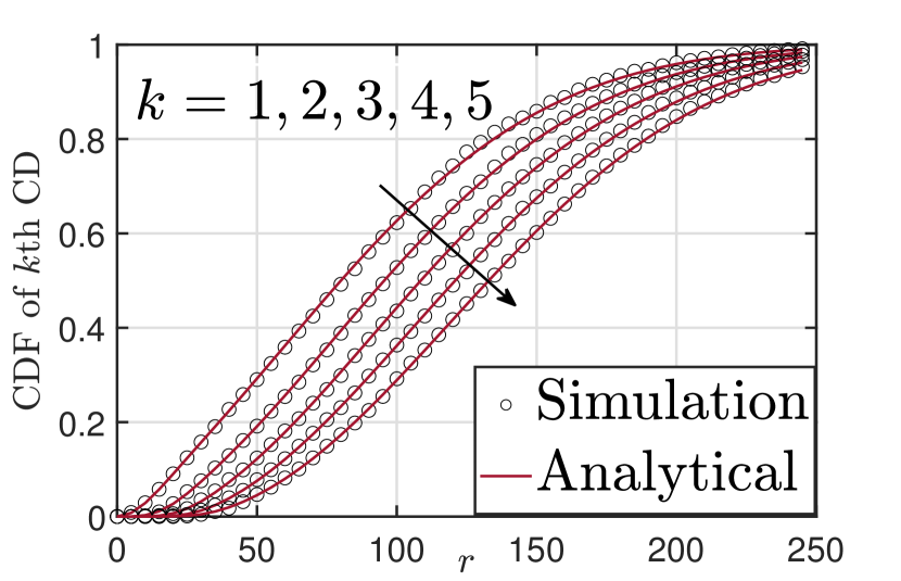
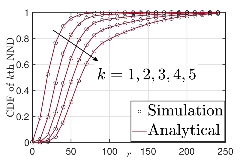
Figure 1: The CDFs of $k$th CD and NND with $\lambda_{\mathrm{p}}=2\times 10^{-5},\overline{m}=5,r_{\mathrm{d}}=50$.

V Relation between CD and NND Distributions

(11) establishes a relation between the CDF of $R_{k}$ and $R^{{}^{\prime}}_{k}$. Note that

$$\lim_{k\rightarrow\infty}\sum\nolimits_{i=0}^{k}q_{j}(r)=1,$$ (12)

and therefore $q_{j}\leq 1$ $\forall$ $j$. This means that the CCDF of $R^{{}^{\prime}}_{k}$ is a linear combination of CCDFs of $\{R_{i},\,\forall i\leq k\}$. Moreover, $q_{j}(r)$ denotes the probability that the typical point has more intra-cluster $j$ points within distance $r$ from it.

V-A The first order stochastic dominance of $R_{k}$ over $R^{{}^{\prime}}_{k}$:

The stochastic dominance of $R_{1}$ over $R^{{}^{\prime}}_{1}$ is proved in [13]. Note that

$$\overline{F}_{R^{{}^{\prime}}_{k}}\!(r) =\sum_{i=1}^{k}q_{k-i}(r)\overline{F}_{R_{i}}\!(r)\leq\sum_{i=1}^{k}q_{k-i}\!(r)\overline{F}_{R_{k}}\!(r)\leq\overline{F}_{R_{k}}(r).$$

This implies the stochastic dominance of $R_{k}$ over $R^{{}^{\prime}}_{k}$ $\forall$ $k$.

V-B Asymptotic results with respect to $r_{\mathrm{d}}$ and fixed $\overline{m}$:

As we decrease the cluster radius $r_{\mathrm{d}}\rightarrow 0$, $\mathcal{A}(r,r_{\mathrm{d}},y)\rightarrow v_{n}r_{\mathrm{d}}^{n}$. Therefore, the CDF of NND simplifies to

$$F_{R^{{}^{\prime}}_{k}}(r)=1-e^{-\overline{m}}\sum_{i=1}^{k}\frac{{\overline{m}}^{k-i}\overline{F}_{R_{i}}(r)}{(k-i)!}.$$ (13)

Similarly, as $r_{\mathrm{d}}\rightarrow\infty$, $\mathcal{A}(r,r_{\mathrm{d}},y)\rightarrow v_{n}r^{n}$. Hence, $\mathcal{P}_{N}(s)\rightarrow\exp{\left(\pi\lambda_{\mathrm{p}}\overline{m}(s-1_{r}^{n}\right)}$ which is the PGF of $N$ for a PPP with density $\lambda_{\mathrm{p}}\overline{m}$. This implies that $k$ CD distribution of MCP also converges to that of PPP. Also, from Theorem 3,

$${\mathcal{P}}^{!\mathrm{o}}_{{N}}(s)=\mathcal{P}_{N}(s)\implies\lim_{r_{\mathrm{d}}\rightarrow\infty}F_{R^{{}^{\prime}}_{k}}(r)\rightarrow F_{R_{k}}(r).$$

VI Applications in Large Wireless Networks

We now discuss two applications to understand how obtained results can be used in the analysis of wireless networks.

VI-A Cellular networks with macro-diversity

To enhance the communication reliability, cellular networks can utilize macro-diversity [18] where a user can receive transmission from multiple BSs. Let us consider a cellular network with BSs deployed as a MCP and a typical user at the origin. We assume that the user can establish a connection to a BS if its distance is less than a certain range $R$, termed connectivity radius. Then, $k$-connectivity probability ($\mathrm{p}_{k}$) is defined as the probability that the user can connect to at least $k$ BS i.e.

$$\mathrm{p}_{k}=\mathbb{P}[R_{k}\leq R]=F_{R_{k}}(R).$$

We are interested in studying the impact of cluster radius on the connectivity probability. Fig. 2 shows the variation of $\mathrm{p}_{k}$ with $r_{\mathrm{d}}$, while keeping $\overline{m}$ constant, to show the impact of clustering. The left extreme $r_{\mathrm{d}}\rightarrow 0$ denotes very high level of clustering and right extreme denotes no clustering (PPP behavior). The main observations are as follows:

$k=1$: $\mathrm{p}_{1}$ always increases with $r_{\mathrm{d}}$ implying that clustering hurts the first connection. This can be shown from the expression of $F_{R_{1}}(R)$. This behavior is observed because higher $r_{\mathrm{d}}$ causes nodes to spread more, making the closest node come within $R$ with higher probability.

$k>1$: An increase in $r_{\mathrm{d}}$ spreads nodes. With $r_{\mathrm{d}}$, the following two competing factors determine $\mathrm{p}_{k}$’s behavior

• if the $k$th closest node belongs to the same cluster of the first closest node, it moves away from $\mathrm{o}$ decreasing $\mathrm{p}_{k}$

• if the $k$th closest node belongs to any other cluster, this node comes closer increasing $\mathrm{p}_{k}$.

If the $\lambda_{\mathrm{p}}$ is low, then first case is more likely, while second case is more likely for high $\lambda_{\mathrm{p}}$. Therefore, $\lambda_{\mathrm{p}}$ determines which one of the two factor dominates. We can observe that, with $r_{\mathrm{d}}$, $\mathrm{p}_{k}$ increases for high $\lambda_{\mathrm{p}}$ and decreases for low $\lambda_{\mathrm{p}}$.

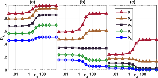
Figure 2: The variation of $k$-connectivity probability with $r_{\mathrm{d}}$ for three values of $\lambda_{\mathrm{p}}$: (a) $3\times 10^{-2}$, (b) $1.3\times 10^{-2}$ and (c) $0.4\times 10^{-2}$. Here $\overline{m}=2$, $R=5$.

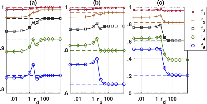
Figure 3: The variation of $\mathrm{f}_{k}$ with $r_{\mathrm{d}}$ for three values of $\lambda_{\mathrm{p}}$: (a) $4.5\times 10^{-2}$, (b) $3.5\times 10^{-2}$ and (c) $2\times 10^{-2}$. Here $\overline{m}=2$, $R=5$.

VI-B Caching in D2D networks

To reduce the file access time and dependency on central servers, nodes in a D2D network can implement caching where each node keeps copies of some popular files locally. A node can access content available at other nodes in its communication range $R$ [19]. To have a right balance between space and latency requirements, only few files are kept at each node while ensuring that all popular files are kept at at least one node of $k$ neighboring nodes. Consider a D2D networks with nodes located as MCP and a typical node $\bm{z}_{\mathrm{o}}$ at the origin requesting a file. The performance of the D2D network can be measured by file retrieval probability or cache hit probability which is defined as the the probability that at least $k$ neighbors are in the communication range of a typical node, i.e.

$$\mathrm{f}_{k}=\mathbb{P}^{\mathrm{o}}[R^{\prime}_{k}\leq R]=F_{R^{\prime}_{k}}(R).$$

Our goal is to understand the impact of $r_{\mathrm{d}}$ on $\mathrm{f}_{k}$. Fig. 3 shows the variation of $\mathrm{f}_{k}$ with $r_{\mathrm{d}}$, while keeping $\overline{m}$ constant, to show the impact of clustering. The dashed lines represent the corresponding $\mathrm{f}_{k}$ for a PPP with density $\overline{m}\lambda_{\mathrm{p}}$. The observed behavior can be justified in the following way. Here also, with $r_{\mathrm{d}}$, there are two competing factors determining $\mathrm{f}_{k}$’s behavior

• if the $k$th neighbor belongs to the typical cluster, it moves away from $\bm{z}_{\mathrm{o}}$ decreasing $\mathrm{f}_{k}$

• if the $k$th neighbor belongs to any other cluster, this nodes comes closer increasing $\mathrm{f}_{k}$.

When $r_{\mathrm{d}}$ is very small, all nodes of the typical cluster are within communication range. Changing $r_{\mathrm{d}}$ doesn’t affect $\mathrm{f}_{k}$.

Now, at lower $\lambda_{\mathrm{p}}$, increasing $r_{\mathrm{d}}$ can spill intra-cluster nodes outside the communication range, decreasing the $\mathrm{f}_{k}$ significantly. Since other clusters are far away, changing $r_{\mathrm{d}}$ doesn’t bring them in communication range. At large $r_{\mathrm{d}}$, nodes start exhibiting the PPP behavior, making $\mathrm{f}_{k}$ independent of $r_{\mathrm{d}}$.

At higher $\lambda_{\mathrm{p}}$, nodes from other clusters start playing role in determining $\mathrm{f}_{k}$. As $r_{\mathrm{d}}$ increases, these nodes can come inside the connection region and become one of $k$ neighbors which increases $\mathrm{f}_{k}$. As $r_{\mathrm{d}}$ further increases, intra-cluster nodes goes outside the connection range decreasing $\mathrm{f}_{k}$ sharply. This fall continues until $r_{\mathrm{d}}$ becomes significantly larger than $R$. After that, intra-cluster nodes are outside the connection radius with high probability. Hence, $\mathrm{f}_{k}$ again starts increasing due to increasing proximity of nodes of other clusters. At large $r_{\mathrm{d}}$, $\mathrm{f}_{k}$ becomes independent of $r_{\mathrm{d}}$ due to limiting PPP nature.

Appendix A

The PGF of $N$ is defined as

$$\mathcal{P}_{N}(s)=\mathbb{E}\left[s^{N}\right]=\mathbb{E}\left[\prod_{\mathbf{Z}\in\Phi}s^{\mathbbm{1}\left({\mathbf{Z}\in\mathcal{B}(\mathrm{o},r)}\right)}\right]$$

which is nothing but the PGFL $\mathcal{G}[v]$ of MCP for $v(\bm{x})=s^{\mathbbm{1}(\bm{x}\in\mathcal{B}(\mathrm{o},r_{\mathrm{d}})(\mathrm{o},r))}$. Further note that

$$v(\bm{x}) =s\times\mathbbm{1}(\bm{x}\in\mathcal{B}(\mathrm{o},r))+1\times(1-\mathbbm{1}(\bm{x}\in\mathcal{B}(\mathrm{o},r)))$$

$$=1+(s-1)\mathbbm{1}(\bm{x}\in\mathcal{B}(\mathrm{o},r)).$$

From the PGFL (1), we get

$$\mathcal{P}_{N}(s)=\mathcal{G}[v] =\exp\left(-\lambda_{\mathrm{p}}\int_{\mathbb{R}^{n}}\left(1-\mathcal{H}_{\bm{x}}[v]\right)\mathrm{d}\bm{x}\right)$$ (14)

with

$$\mathcal{H}_{\bm{x}}[v] =\exp\left(-\lambda_{\mathrm{d}}\int_{\mathcal{B}(\mathrm{o},r_{\mathrm{d}})}\left(1-v(\bm{x}+\bm{y})\right)\mathrm{d}\bm{y}\right)$$

$$=\exp\left(\lambda_{\mathrm{d}}\int_{\mathcal{B}(\mathrm{o},r_{\mathrm{d}})}\left((s-1)\mathbbm{1}(\bm{x}+\bm{y}\in\mathcal{B}(\mathrm{o},r))\right)\mathrm{d}\bm{y}\right)$$

$$=\exp\left(\lambda_{\mathrm{d}}(s-1)\mathcal{A}(r,r_{\mathrm{d}},\|\bm{x}\|)\right).$$ (15)

Replacing the expression of $\mathcal{H}_{\bm{x}}[v]$ in (14) we get

$$\mathcal{P}_{N}(s)=\exp\left(-\lambda_{\mathrm{p}}\int_{\mathbb{R}^{n}}\left(1-e^{\lambda_{\mathrm{d}}\mathcal{A}(r,r_{\mathrm{d}},\|\bm{x}\|)(s-1)}\right)\mathrm{d}\bm{x}\right).$$

Simplifying the above expression, we get the Theorem 1.

Appendix B

The typical point $\bm{z}_{\mathrm{o}}$ is located at the origin $\mathrm{o}$. Under reduced Palm, the number of points falling in the ball $\mathcal{B}(\mathrm{o},r)$ is:

$${N} =\sum\nolimits_{\mathbf{Z}_{i}\in\Phi\setminus\{\bm{z}_{\mathrm{o}}\}}\mathbbm{1}(\mathbf{Z}_{i}\in\mathcal{B}(\mathrm{o},r)).$$

The PGF of $N$ under reduced Palm is

$$\mathcal{P}^{!\mathrm{o}}_{N}(s)=\mathbb{E}^{\mathrm{o}}\left[s^{\sum_{\mathbf{Z}_{i}\in\Phi\setminus\{\mathrm{o}\}}\mathbbm{1}(\mathbf{Z}_{i}\in\mathcal{B}(\mathrm{o},r))}\right],$$

$$=\mathbb{E}^{\mathrm{o}}\left[\prod_{\mathbf{Z}_{i}\in\Phi\setminus\{\mathrm{o}\}}s^{\mathbbm{1}(\bm{X}_{i}\in\mathcal{B}(\mathrm{o},r))}\right]=\mathbb{E}^{!\mathrm{o}}\left[\prod_{\mathbf{Z}_{i}\in\Phi}s^{\mathbbm{1}(\mathbf{Z}_{i}\in\mathcal{B}(\mathrm{o},r))}\right],$$

which is nothing but the PGFL under reduced Palm $\mathcal{G}^{!}_{\mathrm{o}}[v]$ of MCP (given in (10)) for

$v(\bm{x})=s^{\mathbbm{1}(\bm{x}\in\mathcal{B}(\mathrm{o},r_{\mathrm{d}}))}=1+(s-1)\mathbbm{1}(\bm{x}\in\mathcal{B}(\mathrm{o},r_{\mathrm{d}}))$.

Therefore

$$\mathcal{P}^{!\mathrm{o}}_{N}(s) =\mathcal{P}_{N}(s)\ \frac{1}{v_{n}r_{\mathrm{d}}^{n}}\int_{\mathcal{B}(\mathrm{o},r_{\mathrm{d}})}\!\!\!\!\!\mathcal{H}_{-\bm{x}_{\mathrm{o}}}[v]\mathrm{d}\bm{x}_{\mathrm{o}}$$

Now using (15) and converting to polar coordinates, we get

$$\mathcal{P}^{!\mathrm{o}}_{{N}}(s)=\mathcal{P}_{N}(s)\int_{0}^{r_{\mathrm{d}}}e^{(s-1)\lambda_{\mathrm{d}}\mathcal{A}(r,r_{\mathrm{d}},x)}\frac{nx^{n-1}}{r_{\mathrm{d}}^{n}}\mathrm{d}x.$$

Appendix C

Applying PGF-PMF relationship similar to Section III-B and Theorem 3, the PMF of $N$ under Palm is given as

$$\mathbb{P}^{!\mathrm{o}}[N=m]=\frac{1}{m!}\frac{\mathrm{d}^{m}}{\mathrm{d}s^{m}}\mathcal{P}^{!\mathrm{o}}_{N}(s)\left.\vphantom{\frac{3}{4}}\right|_{s=0}$$

$$\stackrel{{\scriptstyle(a)}}{{=}}\frac{1}{m!}\sum_{i=0}^{m}{m\choose i}\mathcal{P}^{(i)}_{N}(0)\int_{0}^{r_{\mathrm{d}}}{(\lambda_{\mathrm{d}}\mathcal{A}(r,r_{\mathrm{d}},x))}^{m-i}e^{-\lambda_{\mathrm{d}}\mathcal{A}(r,r_{\mathrm{d}},x)}\frac{nx^{n-1}}{r_{\mathrm{d}}^{n}}\mathrm{d}x,$$

where $(a)$ is achieved using general Leibniz rule. Using (5) and definition of $q_{j}()$,

$$\mathbb{P}^{!\mathrm{o}}[N=m] =\sum_{i=0}^{m}\frac{1}{m!}{m\choose i}i!\mathbb{P}[N=i]q_{m-i}(r)(m-i)!$$

$$=\sum_{i=0}^{m}\mathbb{P}[N=i]q_{m-i}(r).$$

Now noting that $\mathbb{P}[N=i]=\overline{F}_{R_{i+1}}(r)-\mathbbm{1}(i\geq 1)\overline{F}_{R_{i}}(r)$, we get the desired result.

Appendix D

Now, using Corollary 3.1 in (9), the CDF of $R^{{}^{\prime}}_{k}$ is

$$F_{R^{{}^{\prime}}_{k}}(r)=1-\sum_{m=0}^{k-1}\left[\sum_{i=0}^{m}q_{m-i}(r)\overline{F}_{R_{i+1}}(r)-\sum_{i=1}^{m}\overline{F}_{R_{i}}(r)q_{m-i}(r)\right].$$

Replacing $i^{{}^{\prime}}=i+1$, and $m^{{}^{\prime}}=m+1$ in the first term, enables us to cancel all terms except the term corresponding to $m=k-1$ which gives the desired result.

References

- [1] C. Saha, M. Afshang, and H. S. Dhillon, “3GPP-inspired HetNet model using Poisson cluster process: Sum-product functionals and downlink coverage,” IEEE Trans. Commun., vol. 66, no. 5, pp. 2219–2234, May 2018.
- [2] M. Afshang, H. S. Dhillon, and P. H. J. Chong, “Modeling and performance analysis of clustered device-to-device networks,” IEEE Trans. Wireless Commun., vol. 15, no. 7, pp. 4957–4972, Apr. 2016.
- [3] C.-H. Lee, C.-Y. Shih, and Y.-S. Chen, “Stochastic geometry based models for modeling cellular networks in urban areas,” Wireless networks, vol. 19, no. 6, pp. 1063–1072, Aug. 2013.
- [4] S. M. Azimi-Abarghouyi, B. Makki, M. Haenggi, M. Nasiri-Kenari, and T. Svensson, “Stochastic geometry modeling and analysis of single-and multi-cluster wireless networks,” IEEE Trans. Commun., vol. 66, Oct. 2018.
- [5] Y. Wang and Q. Zhu, “Performance analysis of clustered device-to-device networks using Matérn cluster process,” Wireless Networks, vol. 25, no. 8, pp. 4849–4858, Nov. 2019.
- [6] M. Afshang, H. S. Dhillon, and P. H. J. Chong, “Fundamentals of cluster-centric content placement in cache-enabled device-to-device networks,” IEEE Trans. Commun., vol. 64, no. 6, pp. 2511–2526, Jun. 2016.
- [7] J. Schloemann, H. S. Dhillon, and R. M. Buehrer, “Toward a tractable analysis of localization fundamentals in cellular networks,” IEEE Trans. Wireless Commun., vol. 15, no. 3, pp. 1768–1782, Mar. 2016.
- [8] P. D. Mankar, H. S. Dhillon, and M. Haenggi, “Meta distribution analysis of the downlink SIR for the typical cell in a Poisson cellular network,” in Proc. GLOBECOM, 2019, pp. 1–6.
- [9] X. Zhang and M. Haenggi, “The performance of successive interference cancellation in random wireless networks,” IEEE Trans. Inf. Theory, vol. 60, no. 10, pp. 6368–6388, Jul. 2014.
- [10] K. Pandey and A. K. Gupta, “Coverage improvement of wireless sensor networks via spatial profile information,” in Proc. SPCOM, July 2020.
- [11] M. Haenggi, “On distances in uniformly random networks,” IEEE Trans. Inf. Theory, vol. 51, no. 10, pp. 3584–3586, Sep. 2005.
- [12] J. Andrews, A. Gupta, and H. Dhillon, “A primer on cellular network analysis using stochastic geometry,” arXiv preprint 1604.03183, 2016.
- [13] M. Afshang, C. Saha, and H. S. Dhillon, “Nearest-neighbor and contact distance distributions for Matérn cluster process,” IEEE Commun. Lett., vol. 21, no. 12, pp. 2686–2689, Aug. 2017.
- [14] K. Pandey, H. S. Dhillon, and A. K. Gupta, “On the contact and nearest-neighbor distance distributions for the dimensional Matérn cluster process,” IEEE Wireless Commun. Lett., vol. 9, no. 3, pp. 394–397, Dec. 2020.
- [15] S. Singh, H. S. Dhillon, and J. G. Andrews, “Offloading in heterogeneous networks: modeling, analysis and design insights,” IEEE Trans. Wireless Commun., vol. 12, no. 5, pp. 2484–2497, May 2013.
- [16] M. Haenggi, Stochastic geometry for wireless networks. Cambridge University Press, 2012.
- [17] R. K. Ganti and M. Haenggi, “Interference and outage in clustered wireless ad hoc networks,” IEEE Trans. on Inf. Theory, vol. 55, no. 9, pp. 4067–4086, Aug. 2009.
- [18] A. K. Gupta, J. G. Andrews, and R. W. Heath, “Macrodiversity in cellular networks with random blockages,” IEEE Trans. Wireless Commun., vol. 17, no. 2, pp. 996–1010, Feb 2018.
- [19] D. Malak, M. Al-Shalash, and J. G. Andrews, “Optimizing the spatial content caching distribution for device-to-device communications,” in Proc. IEEE ISIT, 2016, pp. 280–284.