AMM: Adaptive Multilinear Meshes

Abstract

Adaptive representations are increasingly indispensable for reducing the in-memory and on-disk footprints of large-scale data. Usual solutions are designed broadly along two themes: reducing data precision, e.g., through compression, or adapting data resolution, e.g., using spatial hierarchies. Recent research suggests that combining the two approaches, i.e., adapting both resolution and precision simultaneously, can offer significant gains over using them individually. However, there currently exist no practical solutions to creating and evaluating such representations at scale. In this work, we present a new resolution-precision-adaptive representation to support hybrid data reduction schemes and offer an interface to existing tools and algorithms. Through novelties in spatial hierarchy, our representation, Adaptive Multilinear Meshes (AMM), provides considerable reduction in the mesh size. AMM creates a piecewise multilinear representation of uniformly sampled scalar data and can selectively relax or enforce constraints on conformity, continuity, and coverage, delivering a flexible adaptive representation. AMM also supports representing the function using mixed-precision values to further the achievable gains in data reduction. We describe a practical approach to creating AMM incrementally using arbitrary orderings of data and demonstrate AMM on six types of resolution and precision datastreams. By interfacing with state-of-the-art rendering tools through VTK, we demonstrate the practical and computational advantages of our representation for visualization techniques. With an open-source release of our tool to create AMM, we make such evaluation of data reduction accessible to the community, which we hope will foster new opportunities and future data reduction schemes.

1 Introduction

As scientific datasets continue to grow in size and complexity, adaptive representations have become key to enabling interactive analysis and visualization [1]. Such representations can reduce the memory footprint and processing costs of large-scale data by orders of magnitude, often without perceptible degradation of visualization quality or analysis results [2]. However, existing approaches are limited to either compressed representations of regular grids [3, 4] or multiresolution structures, such as octrees and k-d trees [5, 6]. The former typically provide little spatial adaptivity and, thus, do not benefit from the sparsity that is common in scientific datasets, where often only small portions of space are of interest. With few exceptions [4], data is usually stored uncompressed in memory, limiting the overall grid resolution. Spatially adaptive structures overcome this problem by selectively refining regions of interest, resulting in a smaller memory footprint. However, many multiresolution representations imply structural constraints, causing unnecessary refinement in unimportant regions, especially for odd-sized domains like skinny rectangles or L-shapes. Finally, both approaches are limited to their respective notions of fidelity, adapting either numerical precision or spatial resolution.

The recent work of Hoang et al. [7, 8] has demonstrated that combining both concepts — adapting both resolution and precision simultaneously — can provide significant advantages in reduced storage and/or improved accuracy. Unfortunately, there currently exists no data structure that can easily exploit this idea, as precision-based compression methods do not provide spatial adaptivity, whereas multiresolution grids do not generally adapt in precision.

Figure 1: Adaptive Multilinear Meshes (AMM) are a resolution-precision-adaptive representation of uniformly sampled scalar fields. AMM facilitates a flexible spatial hierarchy — to adapt in space — and mixed-precision storage — to adapt in precision. AMM allows creating and comparing data reduction through arbitrary resolution-precision streams and facilitates interfacing with state-of-the-art tools for visualization and analysis. The figure visualizes data reduction after ingesting 8 MB of data through two streams, $\mathcal{S}_{\text{lcf}}$ and $\mathcal{S}_{\text{cen}}$. The smaller renderings on the sides visualize the types of cells (top; type-1 in green and type-2 in pink) and depths of cells (bottom; deeper cells are darker) in AMM’s spatial hierarchy.

Given a lossy data reduction scheme, we address the challenge of representing the resulting data faithfully and without further loss of information, while minimizing the number of cells and vertices in the representation as well as the number of bits to store for each vertex. Unlike existing multiresolution approaches, we enable varying the precision spatially, e.g., features of interest can be represented with more precision bits than the rest. Unlike common compression techniques, we allow adaptive spatial refinement, i.e., prevent representation of large regions of uninteresting space. In this way, our framework leverages both types of reduction to provide gains in the memory footprint not realizable by either type of approach individually.

Furthermore, our approach aims not necessarily for the best compression ratio, but rather for the flexibility of generating, storing, and accessing data at reduced resolution and precision. Since future data will likely increase much more in resolution than in precision, we anticipate that these unique capabilities of our framework will become increasingly more essential to the design, evaluation, and comparison of different data reduction strategies. This work offers an important step toward a potential synergy between resolution adaptivity and precision adaptivity in the future.

The ability to “incrementally” update the reduced representation through streaming of partial data (e.g., in a client-server setting or simply choosing when to stop) offers significant benefits. First, downstream processing can start without waiting for a potentially long decompression step. Second, with fewer vertices and fewer bits per vertex, such downstream tasks can be performed with improved memory efficiency and, thus, can finish significantly faster to provide the user with approximate results that converge over time. Therefore, we focus on scalar fields defined on uniform grids and introduce an adaptive mesh that can be constructed incrementally from arbitrarily ordered datastreams (sequences of complete or partial values).

Built upon a new type of tree, our representation — Adaptive Multilinear Meshes (AMM), see Fig. 1 — utilizes rectangular cuboidal cells to represent multilinear data. AMM does not require a complete global coverage of space but performs minimal refinement to allow isolated regions of interest without needing all surrounding elements, which minimizes the size of the representation. AMM representations can be created using an easy-to-use, open-source tool and exported to the community-standard VTK [9] meshes, making it straightforward to adopt for commonly used visualization and analysis tasks, e.g., with standard and generic tools, such as Paraview [10] and VisIt [11], or with specific rendering approaches [12, 13, 14].

AMM can be constructed through superpositioning piecewise multilinear C⁰ fields in overlapping subgrids. Specifically, we build upon the recent work by Weiss and Lindstrom [15], who use an octree-based approach to encode data using tensor products of linear B-spline wavelets [16], where the basis functions are defined on piecewise multilinear, spatially overlapping stencils. Compared to their work, our representation uses a more-flexible spatial hierarchy that further reduces the mesh considerably, represents vertex values using a mixed-precision scheme, and supports progressive refinement. AMM can also be created by directly reading in arbitrary axis-aligned multilinear cells with values at the corresponding corners, representing continuous as well as discontinuous functions.

Finally, AMM can be constructed through incremental updates using datastreams that update the representation with additional resolution, additional precision, or both. A key novelty in AMM is that it ingests datastreams with arbitrary orderings. Prior work [7] has shown that different analysis tasks may prefer different types of datastreams — some may need more resolution (e.g., gradient computation) whereas others more precision (e.g., histogram computation). All such datastreams, and others that arbitrarily combine resolution and precision, are supported by our representation. In this way, AMM offers a framework to evaluate in a consistent manner the impact and performance of different data reduction strategies (see Fig. 1).

Contributions.   We present AMM, a new resolution-precision-adaptive representation that can ingest arbitrary data orderings and provide an interface to existing tools and algorithms. Specifically, we make the following contributions:

• AMM is a compact, adaptive representation of piecewise multilinear scalar fields. AMM reduces the number of cells and vertices by supporting (1) arbitrary axis-aligned splits through the center to create rectangular cuboidal cells, and (2) incomplete splitting of cells and their optimal resolution with lazy updates. Using a tensor-product wavelet basis, we extend the work of Weiss and Lindstrom [15] and reduce the size of equivalent representations.

• AMM uses a mixed-precision, block-based encoding of values at the vertices, providing superior data reduction than spatial adaptivity alone.

• AMM is the first-of-its-kind adaptive representation that can be updated progressively using arbitrarily ordered datastreams, offering new opportunities to explore dynamic and hybrid data reduction strategies [7, 8].

• For wavelet transforms that require boundary conditions or are defined only for square grids of certain dimensions, we present a novel linear-lifting method to extrapolate the data to avoid discontinuities and artificially large coefficients at the domain boundary, preventing unnecessary mesh refinement.

• We present an open-source implementation of the tool to create and export AMM to standard VTK meshes (github.com/llnl/amm), allowing for its wider adoption and use with state-of-the-art tools.

2 Background and Related Work

Tree-based hierarchies,   such as k-d trees [17, 18] and octrees [19], are among the most popular spatial-subdivision schemes due to their simplicity. Octrees, in particular, have found widespread adoption across diverse domains. They are especially useful when the data contains sparse details, so the smooth-varying regions can be stored at coarser octree levels, thereby reducing storage, e.g., using sparse voxel octrees [20, 21, 22]. Recent approaches have made modifications to traditional octrees to leverage modern computational architectures. For example, OpenVDB [23] increases the tree branching factor to ensure that sibling nodes are stored contiguously in a cache-friendly layout; SPGrid [24] stores octree levels separately as sparse and nonoverlapping grids, taking advantage of virtual memory handling capacities in modern operating systems. Similar to SPGrid, we store per-level vertices separately and aggregate them on demand, but use hash tables instead of the OS’s virtual memory to handle sparsity.

Adaptive mesh refinement (AMR)   [25, 26] is another popular class of multiresolution schemes, especially for simulations. In structured AMR, each resolution level consists of a set of nonoverlapping uniform grids. As the grids can be placed arbitrarily, fine-resolution grids can be used to quickly resolve fine details. An AMR mesh can be either vertex-centered or cell-centered, depending upon where the data points are stored. Although the cell-centered approach is more common, visualizing the resulting mesh requires preprocessing steps, such as remeshing and stitching [27, 28] and ad hoc interpolation [29, 30]. In contrast, our representation is vertex-based, with a principled method for (multilinear) interpolation.

Wavelets   provide a rigorous framework for multiresolution decomposition that is also amenable for data reduction and, thus, is commonly used in visualization frameworks for large data [31, 32, 33, 34]. There also have been works that study data simplification and approximation using wavelet-based subdivision schemes [35, 36], as well as representing multilinear functions using a minimal number of mesh elements to reduce memory footprints [15, 37].

Linsen et al. [37] subdivide cubes into simplices and use linear interpolation for function reconstruction. Weiss and Lindstrom [15] later demonstrated that using multilinear interpolation produces superior quality meshes with respect to approximation error. Conceptually, our representation is most similar to Weiss and Lindstrom’s approach, although AMM is a more general representation. In particular, our framework utilizes rectangular cuboidal cells as opposed to cube-shaped cells (of a standard octree hierarchy) exclusively, thereby significantly reducing memory requirements.

We use linear B-spline wavelets [16] to populate AMM, since multilinear interpolants are at the foundation of many visualization techniques [38, 39, 40, 41]. Sparse grids [42, 43], a common solution for circumventing the curse of dimensionality when solving partial differential equations, also form a piecewise multilinear multiresolution basis and would fit into our hierarchical framework.

Compression techniques.   Beside hierarchical decomposition, data compression is effective at reducing data sizes. Prominent compression methods for scientific data, such as zfp [4], SZ [44], and TTHRESH [45], focus more on reducing data precision through transform/prediction steps followed by quantization of the resulting coefficients or residuals. Compression techniques that reduce resolution have also been investigated. Recently, Ainsworth et al. [46, 47] presented a multigrid approach that offers compression at different levels of the hierarchy. Zhao et al. [48] introduced a multilevel spline-based approach for lossy compression. However, these techniques can support only a one-shot data reduction whereas AMM is designed to handle arbitrary datastreams and incremental updates. Wavelet-based compression [49, 50, 51, 52, 53, 8] often produces progressive bitstreams that improve the data resolution as well as precision. However, such ideas do not provide any adaptive in-memory representation that could be constructed from such streams. This gap is filled by AMM, which complements these wavelet coders by offering a compact in-memory representation for data approximations constructed from compressed bitstreams.

It is not meaningful to directly compare compact meshes, such as the one by Weiss and Lindstrom [15] or AMM, with pure compression techniques, since the former have overheads of embedded data structures needed to support resolution adaptivity, and they also need to put more emphasis on data access speed instead of data reduction alone. Rather than focusing on providing unbalanced comparisons, we consider AMM and compression to be complementary approaches and highlight the flexibility offered by AMM that may be used to leverage compression in the future.

2.1 Octree and Regular Refinement

AMM is based on an advanced tree representation that builds upon the idea of regular refinement of octrees, which are a common way of defining a spatial hierarchy over regular grids. With a slight abuse of notation, we use octree to refer to both octrees (in 3D) and quadtrees (in 2D). An octree is a spatial hierarchy defined on a $d$-dimensional space; it is defined as a collection of $d$-cubes, which form the nodes of the tree. Under regular refinement, a parent node (a $d$-cube) is decomposed into $2^{d}$ child nodes (also $d$-cubes), by splitting each dimension in half. The root node covers the entire domain. The nodes that have no children are referred to as leaf nodes, whereas all others are internal nodes. The number of refinements needed to obtain a given node from the root node defines the depth (also referred to as the level) of the node. An adaptive representation can be obtained by selectively refining the nodes of interest. When an octree is defined over a regular grid, such that the vertices of the grid form the corners of the $d$-cubes, standard representations require the size of the domain (number of vertices in each dimension) to be $2^{L}+1$, where $L$ defines the maximum depth of the hierarchy; the size of a node at depth $\ell$ is given by $s_{\ell}=2^{L-\ell}+1$. The midpoints of the parent node and its facets (i.e., edges, faces) form the vertices of the child nodes, and each child contains one of the vertices of the parent node. Given a regular cubical mesh defined by an octree, we refer to the $k$-dimensional faces of the tree as primal cubes, and to the axis-aligned $(d-k)$-cubes defined by connecting the centers of their adjacent $d$-cubes as dual cubes.

2.2 Multilinear Tensor-Product Wavelets

Wavelet transforms create multiscale data representations. Such representations are defined by translations and dilations of a wavelet basis function, W, which extracts the detail at a given scale, and a scaling basis function, S, which captures the coarse representation after removing the details. Here, W is a high-pass filter whereas S is a low-pass filter that represents the wavelet bases across all remaining scales.

Lifting scheme for linear B-spline wavelet transform.   Given a 1D uniform grid of length $2^{L}+1$, (discrete) wavelet transforms are often implemented in the form of lifting schemes. The forward lifting transform associated with linear B-spline wavelets consists of two phases. The first phase, the w-lift, defines the wavelet coefficient for every odd-indexed vertex on the grid as the prediction residual of the average of its two immediate neighbors from the given function value. The second phase, the s-lift, is then optionally applied to preserve the mean of the function. The s-lift updates the values of the even-indexed vertices by adding a weighted sum of the values obtained in the w-lift. Mathematically, w-lift is $\hat{f}(v_{2i+1})=f(v_{2i+1})-\frac{1}{2}\left[f(v_{2i})+f(v_{2i+2})\right]$, and s-lift is $\hat{f}(v_{2i})=f(v_{2i})+\frac{1}{4}\left[\hat{f}(v_{2i-1})+\hat{f}(v_{2i+1})\right]$, where, $f$ denotes the input function, $\hat{f}$ the wavelet (odd-indexed) and scaling (even-indexed) coefficients, and $v_{i}$ denotes the indexed vertex in the grid. Multiple resolutions of wavelet transforms are obtained by recursively applying lifting steps to the even-indexed vertices at each level. The inverse wavelet transform simply inverts these operations.

When only the w-lift step is performed, the resulting wavelet bases satisfy the Lagrange property, leading to an interpolation of the function, and the corresponding wavelets are commonly called interpolating wavelets. On the other hand, using both the w-lift and the s-lift leads to approximating wavelets. The wavelet synthesis bases for the interpolating and approximating wavelets correspond to piecewise-linear spatial stencils with nodal values $\textbf{{W}}^{I}=[0,1,0]$ and $\textbf{{W}}^{A}=\frac{1}{8}[0,-1,-2,6,-2,-1,0]$, respectively, whereas the stencil corresponding to the scaling function for both types is $\textbf{{S}}=\frac{1}{2}[0,1,2,1,0]$. Wavelet transforms exhibit the two-scale relation [54], i.e., both the scaling and the wavelet functions at a given scale can be expressed in terms of (translated and dilated) scaling functions at the next finer scale. When combined with the piecewise linear nature of the basis functions, the spatial stencils described above produce a hierarchical representation in terms of a regular grid, i.e., a stencil at a given level can be described in terms of the vertices at the next (finer) level.

Multilinear tensor-product wavelets in 2D and 3D.   These ideas can be generalized to higher dimensions by taking the tensor product of the basis functions. Shown by Weiss and Lindstrom [15], a basis function defined by the tensor product of $k$ wavelets and $d-k$ scaling functions (for a $d$-dimensional regular grid) is associated with the midpoint of a $k$-cube in the $d$-dimensional grid. For example, refer to Fig. 6 and note that in 2D the tensor product scaling functions $\textbf{{S}}_{x}\textbf{{S}}_{y}$ are associated with the vertices of the grid, the wavelets $\textbf{{S}}_{x}\textbf{{W}}_{y}$ and $\textbf{{W}}_{x}\textbf{{S}}_{y}$ with the midpoints of edges, and the wavelets $\textbf{{W}}_{x}\textbf{{W}}_{y}$ with midpoints of the square cells. Since the scaling functions for linear B-spline wavelets correspond to linear interpolation, their tensor product corresponds to multilinear interpolation.

3 Adaptive Multilinear Meshes

AMM provides flexible adaptivity in representing uniformly gridded scalar data through a new type of spatial hierarchy that supports more-general splitting operations as compared to existing tree-based hierarchies, such as octrees and k-d trees. Our data structure enables significant reduction of the size of the representation through two novelties: (1) rectangular cuboidal cells, which ensure a tree node is split only along the axes required, and (2) improper nodes, which facilitate partial splitting and representation of a node.

We draw a distinction between nodes of the tree, which define the spatial hierarchy, and cells of the resulting mesh, which are the leaf nodes of the tree after resolving improper nodes (discussed in Section 3.1.3 and Section 4.2.4) that lie partially or completely inside the given domain (as discussed in Section 3.1.1, the tree may cover a larger spatial extent than that of the given data). The corners of nodes/cells form the vertices of the tree/mesh and are associated with function values. The function can be reconstructed anywhere using multilinear interpolation of vertices.

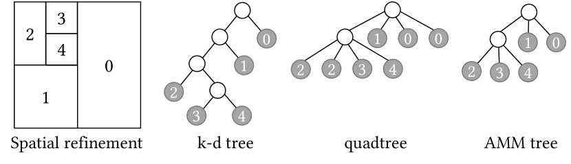
Figure 2: AMM’s tree supports flexible axis-aligned split configurations, which avoids artificially deep hierarchies (like with k-d trees), or an excessive number of subdivisions (like with quad/octrees), which leads to redundant cells and vertices. In this example, the leaf nodes (shaded) in all three trees represent the same partitioning of space.

3.1 Spatial Adaptivity Using a New Tree Data Structure

Spatial hiearchies are commonly created as octrees or k-d trees. For the former, each node (a $d$-cube) is either a leaf node (i.e., no child nodes) or is fully refined along $d$ axes (i.e., $2^{d}$ child nodes). Hence, octrees provide only one degree of freedom: no refinement or full refinement. Similarly, k-d trees, which split a spatial region along a hyperplane, also offer only a binary, axis-based hierarchy, usually alternating through the splitting dimension. Both types of hierarchy are limited in their spatial adaptivity to two configurations only.

In contrast, AMM creates a spatial hierarchy that subdivides a $d$-cube through its center with respect to any arbitrary combination of axes. Hence, the subdivision is restricted neither to a single axis (as in a k-d tree) nor to all axes (as in an octree). This subdivision flexibility facilitates many types of refinement configurations, ultimately allowing us to reduce size of the resulting mesh (see Fig. 2).

3.1.1 Sizes of the Tree and Nodes

Similar to standard approaches, we enforce our spatial hierarchy to sizes that are powers of two plus one and require the root node to represent a $d$-cube, i.e., equal sizes in all dimensions. Given data extents $[X\times Y\times Z]$ in 3D, the spatial extent of the tree and the size (number of vertices in each dimension) of the root node are $2^{L}+1$, where $L=\lceil\log_{2}\left(\max(X,Y,Z)\right)\rceil$ is the maximum depth of the tree. We also borrow the regular refinement operation from octrees, which splits a node (a $d$-cube) with size $s_{\ell}=2^{L-\ell}+1$ is split into child nodes that are also $d$-cubes of size $s_{\ell+1}$. Recall that $\ell$ is called the depth of the node.

The overhead associated with expanding the spatial extent is negligible, since when properly constructed (see Section 4.2), the regions outside the original domain contain a small number of nodes. Furthermore, the expansion offers opportunities for efficient storage and representation of the tree (discussed in Section 3.1.4). Finally, using $2^{L}+1$ sizes also offers a way to avoid the boundary artifacts, where otherwise arbitrary refinement can happen near the boundary of the data domain (see Section 4.3).

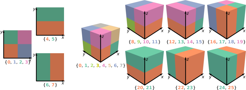
Figure 3: AMM provides flexible spatial adaptivity through arbitrary combinations of axis-aligned subdivisions of a spatial cube (nodes of the underlying tree). The figure shows the different types of child nodes (spatial subdivisions) in 2D and 3D, and their color-corresponded ids. AMM can support any combination of nonoverlapping child nodes, referred to as a valid node configuration, e.g., {0,4,18,25} and {10,11,12,13} in 3D, and, thus, represent more-general configurations of cells, reducing the memory footprint.

3.1.2 Rectangular Cuboidal Leaf Nodes

Toward the goal of creating as few cells as possible, AMM’s leaf nodes are allowed to be rectangular cuboidal in shape whenever possible (i.e., as large as they can be). On the other hand, internal nodes are required to have equal sides (i.e., $d$-cubes only) to favor simplicity and efficiency of traversal. Specifically, as illustrated in Fig. 3, there can be 8 and 26 types of leaf nodes in 2D and 3D, respectively, as compared to 4 and 8 types of “regular” child nodes ($d$-cubes) for the 2D and 3D cases (quadtrees and octrees). Intuitively, the types of rectangular nodes can be enumerated by fixing $k$ dimensions that are not split and splitting the remaining $d-k$ dimensions and counting the combinations of axes that are split and not split. Here, $k$ can be used to categorize the type of nodes. AMM leaf nodes can be type-0 (all $d$ sides equal to $s_{\ell+1}$), type-1 (one side, $s_{\ell}$, longer than the other $d-1$ sides, $s_{\ell+1}$), and type-2 (two equal sides, $s_{\ell}$, longer than the third, $s_{\ell+1}$); type-2 does not exist in 2D. Formally, a penultimate level node in AMM (a $d$-cube) may have $2^{d}+d\sum_{k=1}^{d-1}{2^{d-k}}$ types of child nodes. Here, the first term, $2^{d}$, represents the regular child nodes ($d$-cubes of size $s_{\ell+1}$), and the term in the summation captures child nodes that have $k$ “long” dimensions (cuboids).

A valid node configuration is a subdivision of a node into a set of nonoverlapping child nodes of the same or different types. For example, in 2D, child ids {0,1,2,3} (all type-0) and {1,3,6} (type-0 and type-1), and in 3D, {10,11,12,13} (all type-1) and {0,4,18,25} (type-0, type-1, and type-2), are all valid configurations. Additionally, a leaf node’s configuration, {} (i.e., no subdivision), is also counted as valid. In this context, octrees and k-d trees support only two valid configurations each — either no refinement or full refinement, whereas AMM allows $n_{2}=8$ in 2D and $n_{3}=146$ in 3D unique valid configurations. Both numbers can be derived as $n_{d}=2+\left(d-\sum_{p=1}^{d-1}2^{-p}\right)n_{d-1}^{2}$, with the base case of $n_{0}=0$. Here, $n_{d-1}^{2}$ enumerates the possible combinations of child nodes when a node is split along a single axes, the multiplication by $d$ accounts for all $d$ axes, the expression in the summation subtracts the redundancies, and the constant “2” adds the two configurations for full refinement and no refinement (which get subtracted while removing redundancies). The expression holds true for $n_{1}=2$ as well, i.e., for a 1D binary hiearchy, which has only two configurations — refinement and no refinement.

During the construction of AMM, rectangular cuboidal leaf nodes are created whenever possible. In addition to the regular refinement that splits a node into child nodes, AMM also allows splitting rectangular cuboidal leaf nodes into smaller sibling nodes, when needed. For example, when a 3-cube is split along $x$ axis, only two leaf nodes, 24 and 25, are created, whereas, if the node is split along $x$ and $y$ axes, four leaf nodes, {16, 17, 18, 19}, are created. If the refinement next requires creating leaf node 0, only leaf node 16 is split (along $z$), and the remaining leaf nodes are left untouched, giving the new configuration as {0,4,17,18,19}. Each rectangular leaf node is handled independently, thus preventing any unnecessary splits.

Furthermore, the two halves {24,25} of the node can be split along $y$ and $z$, respectively, leading to the configuration {13,15,16,18}. By allowing creation only of the cells explicitly needed for the representation, AMM’s flexible spatial hierarchy reduces collateral memory usage Fig. 2). Finally, whereas creating similar decomposition using k-d trees is conceivable, k-d trees allow splitting only one dimension at a time, artificially deepening the hierarchy.

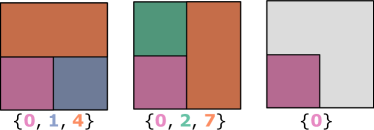
Figure 4: AMM uses improper nodes (right) to preserve ambiguity in refinement (left and middle) by refining a node partially. Here, the child {0} could be created greedily by subdividing the node into {0,1,4} or {0,2,7}, both of which could be suboptimal. Instead, AMM creates only {0} and maintains the remaining region as unresolved until more data is available to make the optimal choice.

3.1.3 Improper Internal Nodes

Although rectangular cuboidal nodes provide highly flexible spatial adaptivity, these additional degrees of freedom may lead to nonessential cells. For example, referring to Fig. 4, consider splitting a 2D node to create the child node {0}. It is possible to split the given node in two ways: splitting along $y$ and then $x$, creating configuration {0,1,4}, or splitting along $x$ and then $y$, giving {0,2,7}. Both these choices can lead to redundant subdivision, depending upon the future requests, e.g., {0,2,7} is not optimal if child {1} is requested next because it will create {0,1,2,3}, whereas {0,1,4} is already sufficient. Rather than making potentially unsuitable choices, AMM defers the subdivision by creating only the requested children. We call a node that is not partitioned fully but has at least one child an improper node.

Partial subdivision within improper nodes creates a subset of child nodes that can be used to represent noncuboidal shapes, e.g., an L-shaped domain. Improper nodes can also be used to represent a region of interest without requiring a complete coverage. Fig. 2 illustrates an example where AMM can reduce the size of the mesh using improper nodes. Improper nodes are our solution to capture the degrees of freedom that have not yet been resolved. By design, the “unresolved” portions of improper nodes do not overlap with any existing child nodes. Therefore, the resulting configurations are also considered valid, e.g., {0} is a valid configuration.

Improper nodes represent a temporary state of AMM to support incremental construction and can be resolved by creating the missing child nodes on demand to support intermediate queries without sacrificing incremental construction (discussed further in Section 4.2.4).

3.1.4 Pointerless Representation of the Tree

AMM uses a pointerless representation of its tree using the notion of location codes, which are commonly used for efficient representation of octrees [55, 56]. Any node within an octree with a maximum depth of $L$ can be uniquely encoded using $d\times L+1$ bits, where $d$ bits are used to locate a child with respect to (the location code of) its parent. In comparison, a location code in AMM requires $d-1$ additional bits per level to support rectangular cuboidal nodes, totaling $(2d-1)\times L+1$ bits per location code. Using 64-bit unsigned integers for location codes, AMM can represent a 3D tree with $L=12$, i.e., data sizes up to $4097^{3}$.

Location codes offer efficient tree traversal as they can be converted into the coordinates of the vertex at the center of the node efficiently using bit shift operations only. For standard octrees, centers of (regular) nodes can be reached by capturing and concatenating every $d$th bit of the location code (from the right) to create the spatial coordinates. AMM follows the same procedure but also discards the $d-1$ additional bits for each level. Since all internal nodes are regular nodes by design, all such discarded bits are zeros. Given a location code, AMM first looks at the $2d-1$ least significant bits, which encode the child id of the node (with respect to its parent). For regular nodes, the standard traversal is sufficient, whereas for rectangular nodes, the standard traversal is used to first find the parent node (a $d$-cube), and then a special case is used to find the correct child. AMM uses location codes also as search keys. Leaf nodes are not stored, and internal nodes are stored as hash maps of location codes to an 8-bit unsigned integer that encodes its node configuration. AMM makes extensive use of hashmaps and switch statements in the code to manipulate node configurations efficiently. Given a valid node configuration and a desired operation (e.g., splitting along $z$ axis), the resulting configuration is known and predefined in the code to optimize computational cost.

Additionally, AMM also stores the vertex values as hash maps from the index to the value of the vertex. Using sizes that are $2^{L}+1$ also offers a way to efficiently encode vertex ids. Whereas the simple and commonly used row-major order requires multiplication and modulo operators to convert between coordinates and index, we leverage the fact that each coordinate requires at most $L+1$ bits and compute the index of a vertex $(x,y,z)$ efficiently using bit-shifts, as $(z<<2(L+1))+(y<<(L+1))+(x)$.

3.2 Precision Adaptivity using Blocks of Vertices

To support mixed-precision representation, AMM stores vertices as blocks of size $4\times 4\times 4$ in 3D and $8\times 8$ in 2D. Values are stored in block floating-point format [4], where each value $v_{i}=2^{e}\times m_{i}$ is expressed with respect to the largest exponent, $e$, in the block. For each block, an exponent is stored only once, and the mantissa bits $m_{i}$ are stored in negabinary format (to avoid special handling of the sign bit) to a fixed precision, i.e., a fixed number of bits, $p$. A block’s precision is defined as the smallest multiple of $8$ (bits) that captures all nonzero bits in every $m_{i}$; each block may have a different precision. AMM also allows spatial adaptivity, i.e., not all vertices in a block may exist. To identify which vertices exist, a 64-bit unsigned integer mask is stored whose bits correspond to vertices in the block. Each block thus comprises a bytestream that encodes the mantissa bits for all existing vertices, the vertex mask (eight bytes), the common exponent $e$ (two bytes), and the precision $p$ (one byte). To index the blocks themselves, AMM uses a hashmap indexed by blocks’ row-major indices.

If a new vertex is added to the block, the bytestream is recreated to insert the new value at its correct location (in order of the local index in the block). We note, however, that updating bytestreams in this way is expensive. For nonprogressive, state-of-the-art compression approaches, the encoding usually happens with the availability of all data, and there is no need to update the bytestream, which provides high throughput. However, supporting incremental updates poses computational challenges because the encoding is dynamic and can change as new values in the block or new bits for existing values are received. In order to support progressive adaptivity, AMM strives to reduce the number of times the bytestream is recreated. As mentioned, AMM represents function values with precision in multiples of bytes, not bits, so that the cost of update is amortized over many bitplanes, i.e., the bytestream does not need to grow with each new bit. We further amortize the computational cost of update through an effective use of staging.

4 Construction of AMM

Although AMM can also be created by simply reading in a collection of multilinear cuboidal cells, in this section, we focus on an important way of creating AMM— using tensor products of biorthogonal linear B-spline wavelets [16].

Here, Section 4.1 describes the relevant properties of the corresponding wavelet basis and draws comparison between AMM and the framework of Weiss and Lindstrom [15]. Section 4.2 presents a practical algorithm to incrementally create AMM through arbitrarily-ordered datastreams of wavelet coefficients. Finally, Section 4.3 discusses a new linear-lifting extrapolation scheme to expand the input data to a $2^{L}+1$ size without boundary artifacts.

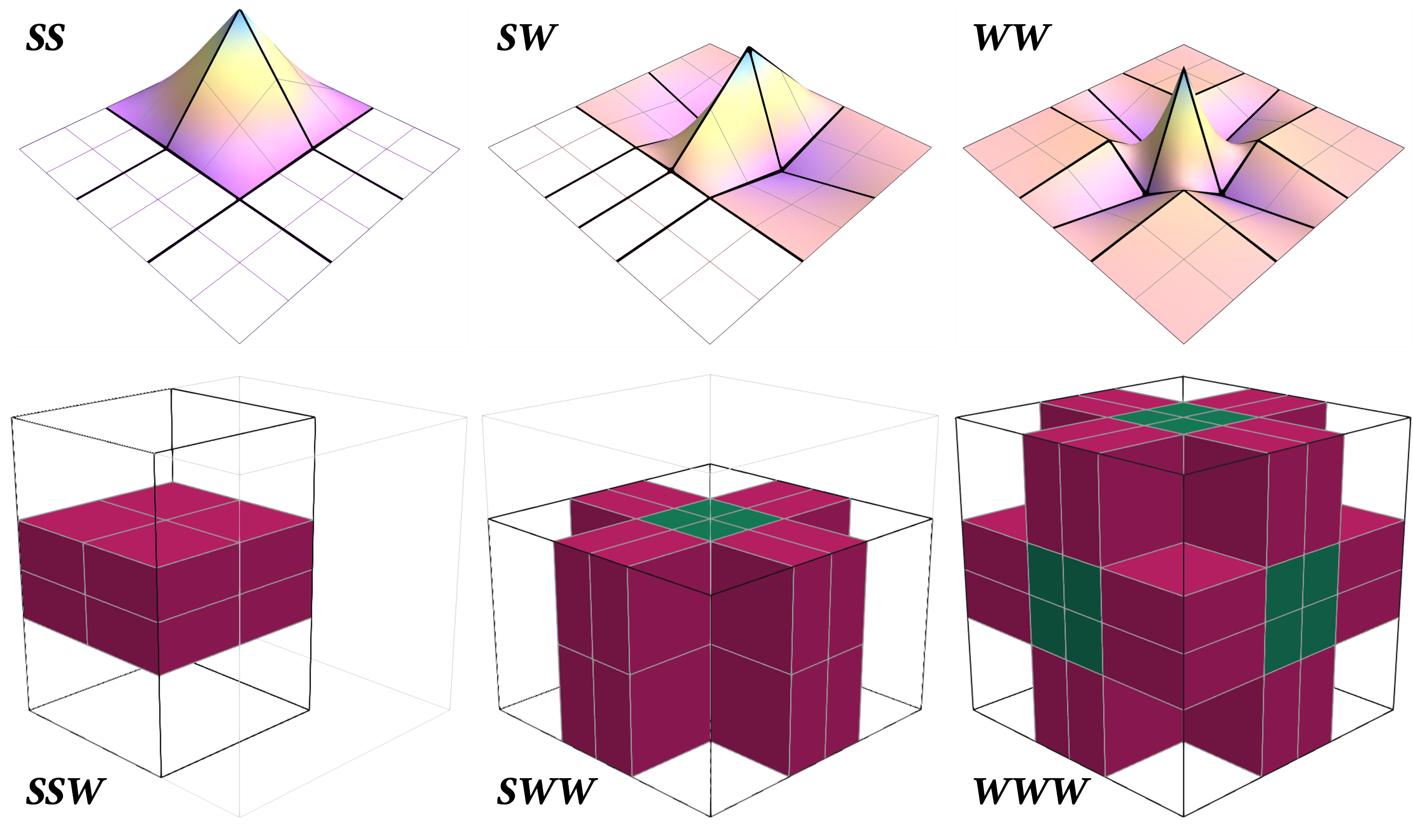
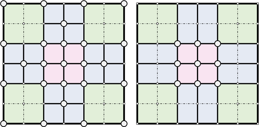
Figure 5: Spatial stencils for bilinear and trilinear tensor-product B-spline wavelets. Top: The 2D stencils are shown with respect to an underlying regular grid, given the cells at two adjacent levels (bold and light lines), with color and height mapped to function value. With respect to the coarser level, the scaling stencil (SS) is associated with vertices, the wavelet stencils (WW) with faces, and mixed stencil (SW and WS) with edges. Bottom: For easier visualization in 3D, only the rectangular cuboidal cells are shown (type-1 = green, type-2 = magenta) within the bounding box of the stencil (black). The scaling stencil (SSS) is not shown.

	Total	[15]		AMM
	#V	#C	#V	#C	#V
SS	25	4	1	4	1
SW	35	12	15	8	3
WW	49	24	25	16	9
SSS	125	8	1	8	1
SSW	175	40	45	16	3
SWW	245	119	63	32	9
WWW	343	160	125	64	27

Figure 6: A WW stencil (placed at the center vertex) as used by Weiss and Lindstrom [15] (left) and AMM (middle). Using rectangular cells and other properties of the stencil, AMM reduces the representation to 9 vertices and 16 cells (4 square green, 4 square pink, and 8 rectangular blue), as compared to 25 vertices and 24 cells [15, Table 1]. The associated table lists such comparisons for all types of stencils in 2D and 3D.

4.1 Wavelet Coefficients and Associated Stencils

As shown in Fig. 6, 2D/3D tensor products of linear B-spline wavelets are associated with “spatial stencils” consisting of multilinear cells at two adjacent levels of refinement. Superposition of such stencils onto a spatial grid is equivalent to performing an inverse transform (the lifting step), but using sparse wavelet coefficients. Previously, Weiss and Lindstrom [15] leveraged these stencils to create reduced and adaptive representations using a restricted set of wavelet coefficients (filtered by magnitude). Nevertheless, since their hierarchy is built upon a regular octree, they are unable to fully exploit the shape of these stencils. Specifically, their representation cannot directly represent the “rectangular portions” of these stencils and instead decomposes such cells into sets of smaller, square cells. This additional decomposition implies a finer mesh to represent sets of cells and vertices that can be trivially interpolated and, therefore, do not provide any additional information. We discuss how AMM’s flexible spatial hierarchy outperforms previous work [15] by reducing the size of the representation.

As an example, consider the approximating wavelet stencil in 2D (WW), illustrated in Fig. 6. When corresponding to a wavelet coefficient at level $\ell$, the stencil is defined on a subgrid at level $\ell+1$ and contains a total of $7\times 7=49$ vertices. Illustrated in Fig. 6, properties of these stencils can be exploited to reduce the number of “effective” vertices (i.e., those that need to be stored to reconstruct the function). According to Weiss and Lindstrom [15], using the zero-valued boundary and the multilinear interpolation of cells in the stencil, only $25$ effective vertices need to be represented.

Our framework further improves this reduction by allowing for rectangular cells using AMM. Specifically, it becomes possible to represent the subdivisions in the axis-aligned neighboring cells of the center point from $4\times 4$ to $4\times 2$, which also removes the need to represent $8$ vertices. Our final representation for this stencil, therefore, contains only $16$ cells and $9$ effective vertices. Unsurprisingly, the gains are substantially higher in 3D; Fig. 6 tabulates the reduction in every type of stencil using our framework.

“Stamping” stencils to the mesh.   Our approach for creating AMM from a given set of wavelet coefficients utilizes a “stamping” procedure for the corresponding spatial stencils. Here, we use the ideas presented by Weiss and Lindstrom [15] to identify the spatial context of a stencil (i.e., cells to be created) using iterators of the primal and dual $k$-cells of regular octree refinement and other standard queries, such as neighhboring cells of a cell and incident cells of a vertex. However, the actual approach of creating these cells is different because of the differences in the spatial hierarchy. To simplify the construction process, AMM exposes an API to create a cell and split a cell along any combination of axes.

The second step in the stamping procedure is the addition of vertices. Given the center vertex of the stencil and its level in the wavelet hierarchy, it is trivial to identify all vertices that need to be updated. As discussed in Section 4.2.3, stencil vertices are also “stamped” into a staging phase and combined with the vertices from coarser and finer levels later in the unstaging step.

4.2 A Practical Approach Toward Creating AMM

Our approach toward creating a resolution-precision-adaptive representation is guided by four goals: (1) the smallest number of cells and vertices that can represent the function faithfully, (2) speed of construction, (3) ability to perform incremental updates through arbitrary data streams, and (4) ability to represent the function using mixed-precision values. To achieve these goals, we utilize three staging phases (see Fig. 7) to create AMM.

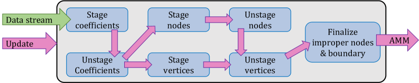
Figure 7: For computational efficiency, construction of AMM is performed using three staging phases. Whereas AMM continues to ingest and stage the incoming datastream (green), this data is processed only when a request to update the mesh is received (e.g., a visualization query). The pink arrows follow the movement of data within the construction pipeline after receiving the update request.

4.2.1 Staging and Unstaging of Wavelet Coefficients

The first challenge is posed by the arbitrary nature of data streams as incoming coefficients may be in any order and may represent complete (all bits) or partial (some bits) values. In the case of partial values, updating the mesh through stamping the corresponding stencils (tree traversals to create nodes and update vertex values) every time a bit is received is wasteful. Even when complete values are to be received, the order of coefficients may require excessive tree traversal, e.g., updating a coarse node in a deep tree requires traversing down and updating the corners of all child nodes.

To mitigate the cost of excessive traversals, AMM collects incoming coefficients without updating the tree. This staging is particularly useful for collecting all bits of the same coefficient and then stamping the stencil only once, preventing redundant operations. At the time of unstaging, these coefficients are sorted coarse-to-fine before stamping to ensure that coarser nodes are created first, preventing the need to propagate the values at the corners of coarse nodes all the way down to the leaf nodes. Finally, this staging process also acts as a filter by discarding any wavelet coefficients whose stencils lie completely outside the data domain (to avoid boundary artifacts, the wavelet transform may be performed on a larger, $2^{L}+1$ domain).

4.2.2 Staging and Unstaging of Tree Nodes

The next optimization our algorithm makes is to prevent unnecessary updates to the spatial hierarchy, i.e., creation and splitting of nodes. Since the stencils of different wavelet coefficients overlap in their spatial extent, different stencils may require updating the same nodes. For example, one stencil may create a node, followed by another that splits it vertically, and another that splits it horizontally.

Instead of processing the tree for each stencil, which requires tree traversals, a few hash map queries, and interpolations to identify the values of the split points, AMM collects all such requests to identify the final state of each node. At the time of unstaging (i.e., when all stencils have been accounted for), each node is processed only once, reducing the overall computational cost.

4.2.3 Staging and Unstaging of Tree Vertices

Whereas the coefficient staging reorders the received data from coarse-to-fine, it can work only on the coefficients received since the last mesh update. During incremental construction, one may already have a deep tree when coarse coefficients are received. The resulting challenge is that any new updates require propagating those changes down to the leaf nodes through recursive interpolation within parent nodes, which quickly becomes computationally prohibitive, especially when nodes at the coarse levels are updated frequently in a deep and/or dense tree.

AMM’s vertex staging mitigates this cost by collecting the updates to vertex values and storing them separately by their level in the tree because vertex updates corresponding to a given level are additive. At the time of unstaging, the tree is traversed down only once for each node updated in the current stage. During this traversal, the corners of a given node are multilinearly interpolated to add to the values of all corners of all child nodes — the corners of the child nodes that are also the corners of the parent node do not need this update. Temporary caches are used to prevent duplicate updates to a vertex for each of its incident nodes.

Mixed-precision representation of vertex values.   The unstaging of vertices naturally separates the vertex values that are created/modified during the current staging/unstaging step from those that existed before. The final task in the vertex unstaging is to combine the two sets of vertex values to give the final and correct values. At this time, if a mixed-precision representation is requested, the vertex values aggregated from the current stage are finalized into the bytestream representation of the vertex values.

4.2.4 Finalization of Improper Nodes and Boundary Nodes

As described earlier, AMM uses improper nodes to preserve unresolved degrees of freedom. However, since typical analysis and visualization tasks expect a complete coverage of space, any improper nodes in the tree must be resolved before preparing the mesh for use. Improper nodes may be resolved by simply creating additional child nodes (by design, these will be leaf nodes of the tree) and associated vertices. AMM preserves the current state of the tree by storing these additional leaf nodes and vertices in a separate and temporary data structure that is used only to respond to the query at hand, without sacrificing the improper nodes for incremental construction.

Furthermore, the underlying tree may also have a larger spatial extent than the given data, in which case there may exist no leaf nodes whose boundary aligns with the boundary of the data domain. In such cases, it is straightforward to identify the leaves that exist across the data boundary and split them using multilinear interpolation to create cells and vertices for the output mesh. Similar to the case of improper nodes, the boundary leaf nodes and the additional vertices are also stored in a temporary data structure to not affect the state of the tree. The AMM API abstracts these temporary data structures, allowing the application to use the mesh directly through cell and vertex iterators and accessors.

4.3 Data Extrapolation Using a Linear-Lifting Scheme

Since wavelet transforms are computed for power-of-two sized grids, their practical application often requires extending the signal to suitable lengths. Whereas several approaches exist for this extension (e.g., zero padding, linear extrapolation, and symmetric extension), each is associated with different types of boundary artifacts, such as discontinuity and nonsmoothness, that lead to large wavelet coefficients, which may not be conducive to the application. For AMM, these artificial coefficients typically result in unnecessary refinement, inflating the memory footprint significantly and needlessly.

Here, we present a new, linear-lifting approach to extend the input function at the boundary to avoid such artifacts and reduce the number of unneccesary cells near the boundary. Conceptually, we perform the usual lifting steps everywhere in an extended domain of size $(2^{L}+1)^{d}$, but assign values lazily to grid points outside the original domain, $[X\times Y\times Z]$ (see Section 3.1.1). Denoted symbolically as (*--*--*), the w-lift step updates the value at the center using the adjacent ones. With respect to the original and extended domains, there exist four possible scenarios: (x--x--x), (x--x--o), (x--o--o), and (o--o--o), where x represents a grid point within the original domain whereas o has an uninitialized value due to being outside the original domain (but within the extended domain). In the first case, all three relevant grid points exist within the original domain and the standard w-lift can be applied. In the second case, we linearly extrapolate the two known values to assign a value to the rightmost grid point when needed, resulting in a zero-valued wavelet coefficient. For the third and the fourth case, we set the wavelet coefficient to zero but defer setting the value for the rightmost sample to an extrapolation step on some coarser level. Furthermore, s-lift is applied only to values that have been initialized — standard step for the first case, but no effect for the remaining three. With this scheme, uninitialized grid points are given values such that when they are used for lifting, the resulting wavelet coefficients are always zero. Table I illustrates our approach using a concrete 1D example.

Input function	56	8	48	44	32	8
Level 1: Extrapolate	56	8	48	44	32	8	-16
Level 1: Forward w-lift	56	-44	48	4	32	0	-16
Level 1: Forward s-lift	45	-44	38	4	33	0	-16
Level 2: Extrapolate	45		38		33		-16		-65
Level 2: Forward w-lift	45		-1		33		0		-65
Level 2: Forward s-lift	45		-1		33		0		-65
Coefficients stored in memory	45	-44	-1	4	33		-16		-65
Level 2: Insert w-coefficients	45		-1		33		0		-65
Level 2: Inverse s-lift	45		-1		33		0		-65
Level 2: Inverse w-lift	45		38		33		-16		-65
Level 1: Insert w-coefficients	45	-44	38	4	33	0	-16	0	-65
Level 1: Inverse s-lift	56	-44	48	4	32	0	-16	0	-65
Level 1: Inverse w-lift	56	8	48	44	32	8	-16	-41	-65
Extrapolated function	56	8	48	44	32	8	-16	-41	-65

TABLE I: Our linear-lifting approach extrapolates a 6-point function using two levels of transform with integer arithmetic. A (forward) lifting phase begins with linear extrapolation (pink), followed by w-lift (brown) and s-lift (blue). Inverse lifting extends the input function to 9 points, but only 7 coefficients are stored for full reconstruction. Note that the extrapolated function is different from one obtained via simple linear extrapolation in the last two elements.

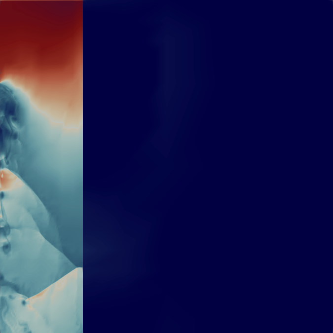
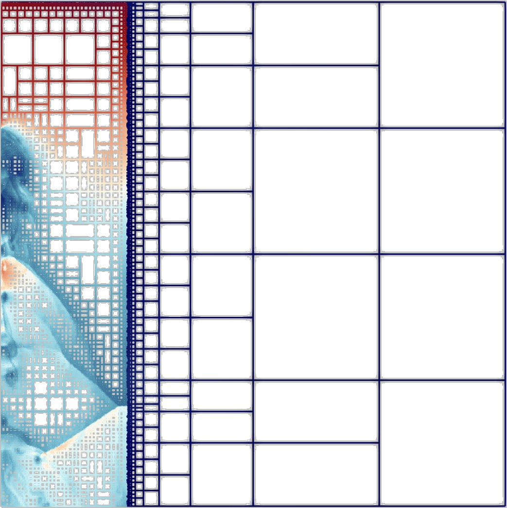
(a) Zero padding
(7997, 9918, 4664)

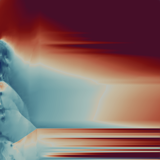
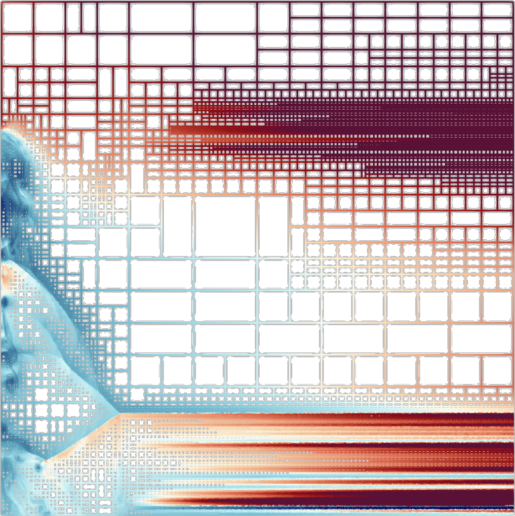
(b) Linear extrap.
(6263, 34742, 19007)

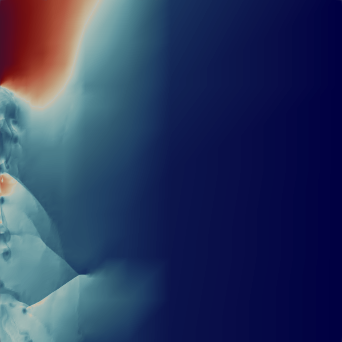
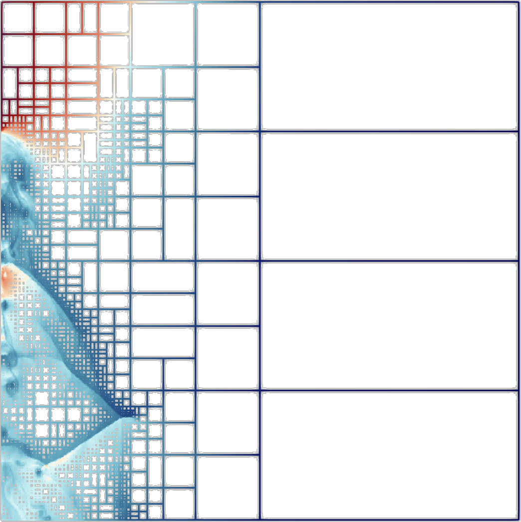
(c) Linear-lifting
(6263, 6342, 2965)

Figure 8: Function extensions (top) and the corresponding meshes (bottom) for a shockwave defined on $[256\times 1024]$ domain and extrapolated to $[1025\times 1025]$ using different methods. The associated metrics are number of (cells, leaf nodes, internal nodes). Zero padding introduces artificial discontinuities at the boundary of the input domain (notice the vertical blue streak of finest-level cells). Linear extrapolation maintains smoothness near the boundary, but can create discontinuities farther out from the original domain. Our linear-lifting approach avoids artificially large wavelet coefficients at the boundary and in the extrapolated region.

Our scheme differs from simple linear extrapolation in that it interleaves the potential linear extrapolation steps described above with lifting steps. Simple linear extrapolation does not ensure smoothness along dimensions orthogonal to the one being extrapolated, while also failing to correct for the nonlinear reconstruction introduced by s-lift steps. In contrast, by interleaving lifting steps with extrapolation steps across the hierarchy and across spatial dimensions, our method ensures smoothness in the extended function both across the boundary of the domain as well as across all dimensions (see Fig. 8). Naive linear extrapolation is also entirely local as it depends only on the last two values near the domain boundary, whereas our method extrapolates at multiple scales and therefore is globally influenced.

In the example from Table I, the extrapolated function is longer than the original function by three elements unlike the traditional wavelet transform, where the two functions have the same length. However, in practice, the inverse lifting steps are never performed, and thus the extrapolated function is never explicitly computed or stored. We do need to store the potentially extrapolated value at each lifting step to support perfect reconstruction, but this requires storing at most a single extra value along each dimension of the original domain, as the same slot can be reused on the next coarser transform level without compromising reconstruction using inverse lifting steps. Since the wavelet coefficients in the extrapolated domain are all zero, in the resulting mesh, AMM’s adaptivity allows the overhead (the extra cells and vertices) to remain small, as seen in Fig. 8c.

5 Evaluation

In our evaluation, we focus on the three design goals of AMM: adaptivity in spatial resolution, adaptivity in precision, and incremental construction, and consider the size of the resulting representation, the reconstruction quality, and the time it takes to compute AMM.

We report the size of our adaptive representation in terms of the number cells and vertices; we also report the approximate memory footprint of the representation by counting eight bytes for each cell and vertex (to store indices) and the number of bytes used (one to eight) to represent function values, but ignore the additional overhead of data structures such as hash maps. To quantify the quality of a reconstructed function $\hat{f}$ against the original function $f$, we measure the peak signal-to-noise ratio, PSNR $=20\log_{10}\left((f_{\max{}}-f_{\min{}})/2\right)-10\log_{10}\left(\sum{(f-\hat{f})^{2}}/N\right)$, where $N$ is the total number of samples in the given data.

Datastreams.   In this work, we consider six types of datastreams. We borrow four datastreams from Hoang et al. [7] — “by-magnitude” ($\mathcal{S}_{\text{mag}}$), “by-level” ($\mathcal{S}_{\text{lvl}}$), “by-bit-plane” ($\mathcal{S}_{\text{bit}}$), and “by-wavelet-norm” ($\mathcal{S}_{\text{wav}}$). Here, $\mathcal{S}_{\text{mag}}$ is a resolution stream since it transmits complete coefficients, which are ordered by their magnitude. Streams $\mathcal{S}_{\text{lvl}}$, $\mathcal{S}_{\text{bit}}$ and $\mathcal{S}_{\text{wav}}$ are precision streams since they may transmit bits of a coefficient separately; $\mathcal{S}_{\text{lvl}}$ orders coefficients by level in the wavelet hierarchy (coarse to fine) but transmits the bits after discarding leading zeros; $\mathcal{S}_{\text{bit}}$ picks the bits in order of bit plane (most significant to least significant); and $\mathcal{S}_{\text{wav}}$ combines the functionality of $\mathcal{S}_{\text{bit}}$ and $\mathcal{S}_{\text{lvl}}$ to order the bits based on both the bit plane and the wavelet basis on the subband of the coefficient. We consider two additional resolution streams — “by-level-coeff”, ($\mathcal{S}_{\text{lcf}}$), which transmits complete coefficients ordered by level in the wavelet hierarchy; and “by-coeffient-energy”, ($\mathcal{S}_{\text{cen}}$), which orders the coefficients based on both the magnitude of the coefficient and the norm of the wavelet basis function for the corresponding subband.

Interfacing with other tools for visualization.   Although several visualization tools support spatially adaptive representations, precision adaptivity is generally not well supported due to both software and hardware limitations, and the data is typically inflated first to full-precision (floats or doubles) before visualization. Whereas utilizing AMM directly at reduced precision remains a task for the future, currently AMM facilitates analysis and visualization by providing a simple interface to the visualization toolkit (VTK) [9]. It is straightforward to output AMM as a VTK unstructured grid, which can be used with standard tools, such as Paraview [10], VisIt [11], and OSPRay [14], as well as to support hardware-accelerated rendering [12, 13].

Volume renderings of the original, uniform-grid data in this paper are generated using nanovdb [57], and those of AMM are generated using the GPU-based unstructured volume rendering approach of Morrical et al. [12], which employs fixed function tree traversal units to efficiently locate and interpolate unstructured elements. For this work, we improved the performance of this approach by leveraging the properties of AMM — axis-aligned cells with predictable sizes. Given axis-aligned cells, we invert the per-vertex interpolants using analytical voxel-trilinear interpolation instead of the root-finding method required for general, curved hexahedra. Likewise, memory bandwidth is reduced by reading only two, diagonally opposite vertices instead of all eight as done for arbitrary hexahedra.

Using these tools, we compare the performance of volume rendering for the original data and AMM in terms of the memory footprint and rendering time (as milliseconds per frame). Whereas our current pipeline demonstrates the computational benefits of AMM (small meshes with axis-aligned cells) using external tools, we envision a more-integrated visualization directly using AMM in the future.

5.1 Evaluation of Spatial Hierarchy

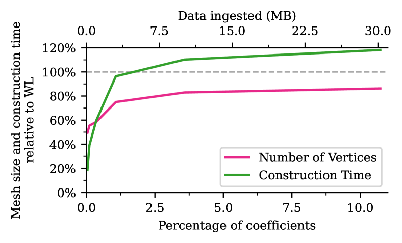
Figure 9: In this example, AMM improves the data reduction by 20%–50% as compared to the framework of Weiss and Lindstrom [15], while taking up to 20% more time to construct. However, in the relevant levels of reduction ($<$2% of the coefficients), AMM provides significant improvement.

First, we compare AMM’s adaptivity in spatial resolution to the recent work of Weiss and Lindstrom (WL) [15]. To set up this comparison, we note that the competing tool creates a reduced representation by filtering wavelet coefficients by magnitude, akin to the $\mathcal{S}_{\text{mag}}$ stream. Therefore, for this comparison, AMM was generated without the incremental mode, i.e., consuming all filtered data at once.

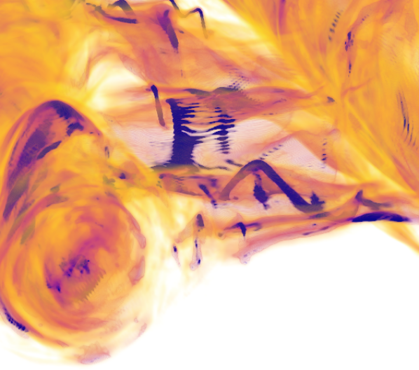
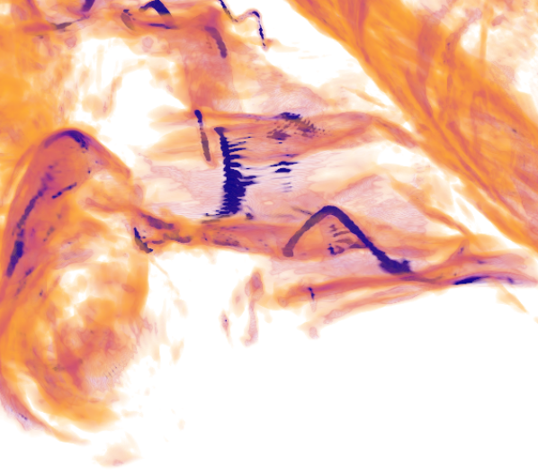
Figure 10: Volume rendering of the magnetic reconnection event dataset at full resolution (left, 512 MB) and AMM (right, 9.86 MB) are shown, highlighting the flexibility of AMM to handle different types of (dense vs. sparse) datasets and still highlight important features therein.

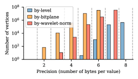
Figure 11: Using mixed-precision format for vertex values, AMM provides additional savings in the representation. The figure compares reduced volumes (upper row) with the original, and also provides analysis on the distribution of precision (lower row) in the reduced data as a histogram and as volume renderings (darker color means low precision).

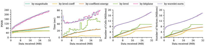
Figure 12: AMM provides a simple and consistent framework to create and compare reduced representations using different resolution and precision streams. The plots compare six streams and show that two precision streams (by-bitplane and by-wavelet-norm) drastically outperform others in terms of quality, but at commensurately large mesh sizes.

To concisely present the comparisons, Fig. 9 reports the relative size and time to compute AMM with respect to WL. Here, the horizontal axis captures an unusually large range of coefficients — given the nature and size of this dataset, good quality reconstructions can be obtained within the first 1–2% of the coefficients (also shown by WL [15, Fig. 9]). Within this more reasonable range, AMM produces about 20–50% smaller meshes (not even counting cells) while taking about the same time for construction. Once the mesh is refined further, AMM’s gains stabilize, since at this time, there are fewer rectangular nodes, but it still takes longer to process the more sophisticated hierarchy.

For comparisons, we added a “standard hierarchy mode” in AMM, where rectangular and improper nodes are disallowed. In the absence of a standard output mesh from WL, the next result uses AMM to create meshes both with and without our proposed hierarchy, with the latter acting as a proxy for [15]. Next, we reduce a $[512\times 512\times 512]$ float32 dataset (512 MB), which represents a magnetic reconnection event in relativistic plasmas [58], to roughly the same footprint using both techniques (about 10 MB each). Without using rectangular nodes, one can process only 8192 largest coefficients, giving a mesh with 9.94 MB footprint. On the other hand, with AMM’s hierarchy, it is possible to utilize 23,040 coefficients with a 9.86 MB footprint, which allows capturing features of interest in the data (see Fig. 10).

Next, we consider the entropy field from a Richtmyer-Meshkov instability simulation [59] and use AMM to compare the reduction obtained using $\mathcal{S}_{\text{lcf}}$ and $\mathcal{S}_{\text{cen}}$. As shown in Fig. 1, $\mathcal{S}_{\text{lcf}}$ (which streams the data in order of wavelet subbands) sweeps through space rather evenly, refining large regions to the same depth. On the other hand, $\mathcal{S}_{\text{cen}}$ (which scales the coefficients by wavelet function norm) allows capturing more quickly the turbulent regions of interest. When streamed for 8 MB each, both streams create different representation sizes, with $\mathcal{S}_{\text{cen}}$ creating an almost 4$\times$ denser mesh. Not only does AMM provide improved data reduction due to its subdivision flexibility, it also facilitates comparing different modes of data reduction easily and through a consistent interface. For this comparison, creating AMM using $\mathcal{S}_{\text{lcf}}$ and $\mathcal{S}_{\text{cen}}$ took 72.5 s and 86.1 s, respectively. Volume rendering of the reduced meshes achieved 22.2 ms and 19.7 ms per frame, with peak memory consumption 2.13 and 2.71 GB, respectively. Comparing these numbers with 31.9 ms per frame and 35.07 GB for the original data demonstrates the computational benefits of AMM.

5.2 Evaluation of Mixed-Precision Representation

To demonstrate mixed-precision capabilities in AMM, we consider the three precision streams introduced above ($\mathcal{S}_{\text{bit}}$, $\mathcal{S}_{\text{lvl}}$, and $\mathcal{S}_{\text{wav}}$) and use a $[2025\times 1600\times 400]$ float64 dataset from the simulation of a lifted flame. We stream 4 MB data (partial coefficients) through these streams and create AMM. Referring to the histogram plot in Fig. 11, we note the distribution of precision captured by AMM. Whereas all streams show a wide distribution, $\mathcal{S}_{\text{bit}}$, in particular, represents several vertex values using two bytes only. Using AMM, it is straightforward to also highlight the differences between the precision distribution visually by rendering it as a volume on the mesh (as shown in the figure for $\mathcal{S}_{\text{lvl}}$ and $\mathcal{S}_{\text{bit}}$). Here, we observe, unsurprisingly, that $\mathcal{S}_{\text{lvl}}$ provides a wider spatial coverage but with lower precision, whereas $\mathcal{S}_{\text{bit}}$ invests bits heavily based on spatial resolution. Finally, the top row of the figure visualizes the resulting volumes and compares the reduced data with the original dataset at full resolution and full precision.

Figure 13: Visual comparison of data reconstructed after streaming 8 MB for each of the six streams against the original, full-resolution data. The numbers at the bottom right provide the approximate memory footprint of the respective meshes.

5.3 Evaluation of Incremental Updates

Finally, we demonstrate the incremental construction of AMM using different types of streams. Here, we work with the Rayleigh-Taylor instability [60] data defined using float64 values on a $[384\times 384\times 256]$ grid. AMM was created for a stream of 32 MB in chunks of 1 MB, i.e., mesh update requests were sent after every 1 MB. Fig. 12 shows the evolution of the representation with respect to these streams in terms of the reconstruction quality (PSNR), time to update the mesh for each chunk, and the size of the resulting mesh (number of cells and vertices). First, we note $\mathcal{S}_{\text{mag}}$ and $\mathcal{S}_{\text{cen}}$ provide almost equivalent reconstruction and performance, because the two streams are quite similar and differ by a scaling factor only, which appears to be nonconsequential for this particular dataset. Next, we look at $\mathcal{S}_{\text{lcf}}$ and $\mathcal{S}_{\text{lvl}}$, which although providing almost equivalent reconstruction quality, refine the mesh very differently. Whereas $\mathcal{S}_{\text{lvl}}$ creates larger mesh sizes and, therefore, is slower to compute, the result indicates that $\mathcal{S}_{\text{lcf}}$ should be the choice of stream among the two. Finally, we observe that, as expected, $\mathcal{S}_{\text{bit}}$ and $\mathcal{S}_{\text{wav}}$, both precision streams, refine the mesh drastically from the beginning by transmitting the most significant bits for most of the turbulent domain, thus not only creating a dense mesh but also providing a much higher quality. By providing such analysis in a consistent manner, AMM facilitates, for the first time, comparing such datastreams in a much more scalable manner than before [7]. Finally, we leave the reader with Fig. 13 to observe the visual quality of the resulting representations for each of the streams.

6 Conclusion and Discussion

In this paper, we present a resolution-precision-adaptive representation that can ingest arbitrary datastreams progressively to provide an interface to existing tools and algorithms. By representing uniformly sampled, scalar-valued data as piecewise multilinear functions using tensor products of linear B-spline wavelets, we produce meshes based on a flexible spatial hierarchy to reduce the size of the mesh and demonstrate faithful reconstruction. AMM uses a mixed-precision representation of function values to further reduce the memory footprint and to facilitate precision adaptivity. Mixed-precision AMM can also be used to trim down superfluous bits in the (full-precision) coefficients received through spatial streams. Currently, AMM’s mixed-precision mode provides a lossless representation, but it is straightforward to expand this framework to achieve lossy reduction by dropping additional bits within acceptable error.

AMM provides a VTK interface through output files, which still somewhat introduces additional overhead in using AMM representations. In the future, we would like to expand our framework to expose an improved API with efficient iterators, accessors, and common visualization queries, such as point queries and contouring, which will facilitate leveraging this framework directly for visualization.

The current implementation of AMM is serial and CPU-based. Whereas it is easy to conceive porting key operations to GPU kernels and/or to a distributed algorithm, the primary challenge appears to be reducing data movement across host and device or across MPI ranks, especially in a streaming setting where it is not known a priori which parts of the tree will be updated. Addressing these challenges offers interesting directions for future research.

We have also identified several opportunities for further improvement in the performance of AMM creation. Most notably, the stamping process for vertices requires tree traversals and is the key bottleneck in further scaling. On the other hand, the lifting process is a standard and efficient technique for inverse transforms, but works with dense data (coefficients on uniform grid). In the future, we will explore the possibilities of utilizing the lifting approach for sparse data (restricted coefficients) and their stencils.

When compared to state-of-the-art compressors, such as zfp or SZ, AMM does not offer competitive rate-distortion curves, since it does not currently employ sophisticated compression to further reduce the memory footprint of the adaptive mesh. On the other hand, such compressors do not reduce the number of vertices and cells and, thus, do not benefit the performance of downstream tasks most of the time. In contrast, by reducing the number of vertices and cells in the representation, AMM offers significant computational advantages during traversal; current work demonstrates about 50% faster volume rendering. Compared to the technique closest to our own [15], AMM produces significantly smaller meshes (20–50% gain) at the same data quality. An important research direction for the future is to combine the best of AMM and compression, e.g., by utilizing zfp to replace the mixed-precision, block-based representation of vertices currently used by AMM.

Finally, a key enabling technology in AMM is the support for incremental updates using arbitrary sequences of data. By relaxing the assumption that the data must be ordered in specific, predefined ways, we aim to position our open-source tool (github.com/llnl/amm) as a standard framework to explore and evaluate the reduction of data in the space of precision and resolution, ultimately resulting in next-generation data reduction techniques.

Harsh Bhatia is a Computer Scientist at the Center for Applied Scientific Computing at Lawrence Livermore National Laboratory. His research spans broad areas of visualization and computational topology, ML-based approaches, high-performance computing, and workflow technologies, with special focus on scientific data. Prior to joining LLNL, Harsh earned his Ph.D. from the Scientific Computing and Imaging Institute at The University of Utah in 2015, where he developed mathematical and combinatorial techniques for feature extraction for vector fields.

Duong Hoang is a Ph.D. student in computer science at the Scientific Computing and Imaging (SCI) Institute, University of Utah. Before joining Utah, he obtained Bachelor and Masters degrees in computer science from the National University of Singapore. His research interests include data compression, scientific data visualization and analysis, computer graphics and scientific computing.

Nate Morrical is a Ph.D. student at the University of Utah, intern alumni from the NVIDIA OptiX team and Pixar’s RenderMan group and a current member of the Scientific Computing and Imaging Institute (SCI). His research interests include high-performance ray-tracing frameworks and computing, scientific data visualization, computational geometry, and real-time ray tracing. Before joining SCI, Nate received his B.S. in computer science from Idaho State University, where he researched interactive computer graphics and computational geometry.

Valerio Pascucci received the EE laurea (master’s) degree from the University La Sapienza, Rome, Italy, in December 1993, as a member of the Geometric Computing Group, and the PhD degree in computer science from Purdue University, in May 2000. He is a faculty member at the Scientific Computing and Imaging (SCI) Institute, University of Utah. Before joining SCI, he served as a project leader at the Lawrence Livermore National Laboratory (LLNL), Center for Applied Scientific Computing (from May 2000) and as an adjunct professor at the Computer Science Department of the University of California, Davis (from July 2005). Prior to his tenure at CASC, he was a senior research associate at the University of Texas at Austin, Center for Computational Visualization, CS, and TICAM Departments. He is a member of the IEEE.

Peer-Timo Bremer is a member of technical staff and project leader at the Center for Applied Scientific Computing (CASC) at the Lawrence Livermore National Laboratory (LLNL) and Associated Director for Research at the Center for Extreme Data Management, Analysis, and Visualization at the University of Utah. He also serves on the research council of the Data Science Institute and as the ASCR point of contact for Data science. His research interests include scientific machine learning, large scale data analysis, topological techniques, and visualization. Prior to his tenure at CASC, he was a postdoctoral research associate at the University of Illinois, Urbana-Champaign. Peer-Timo earned a Ph.D. in Computer science at the University of California, Davis in 2004 and a Diploma in Mathematics and Computer Science from the Leibniz University in Hannover, Germany in 2000. He is a member of the IEEE Computer Society and ACM.

Peter Lindstrom is a Computer Scientist at the Center for Applied Scientific Computing at Lawrence Livermore National Laboratory, where he leads several research efforts that span data compression, scientific visualization, and scientific computing. He received a Ph.D. in computer science from Georgia Institute of Technology in 2000 and B.S. degrees in computer science, mathematics, and physics from Elon University in 1994. Peter previously served as Editor in Chief for Graphical Models, Associate Editor for IEEE Transactions on Visualization and Computer Graphics, and Paper Chair for IEEE VIS. He is a Senior Member of IEEE.

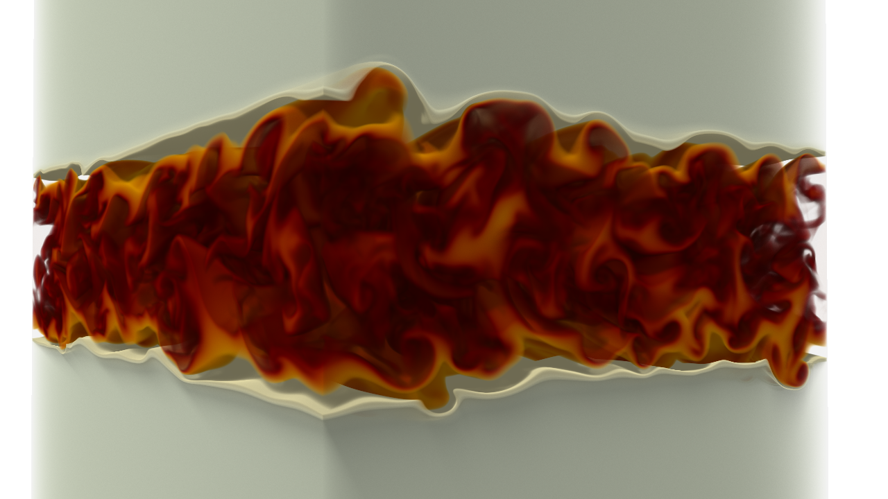
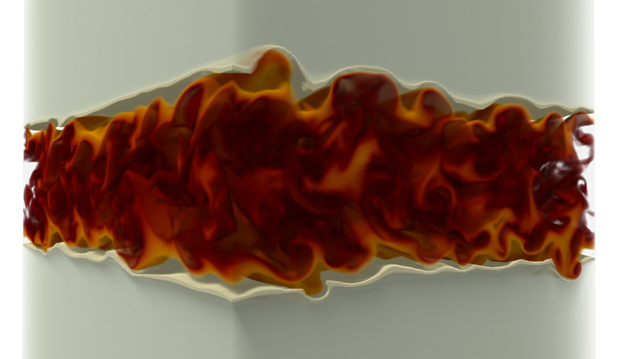
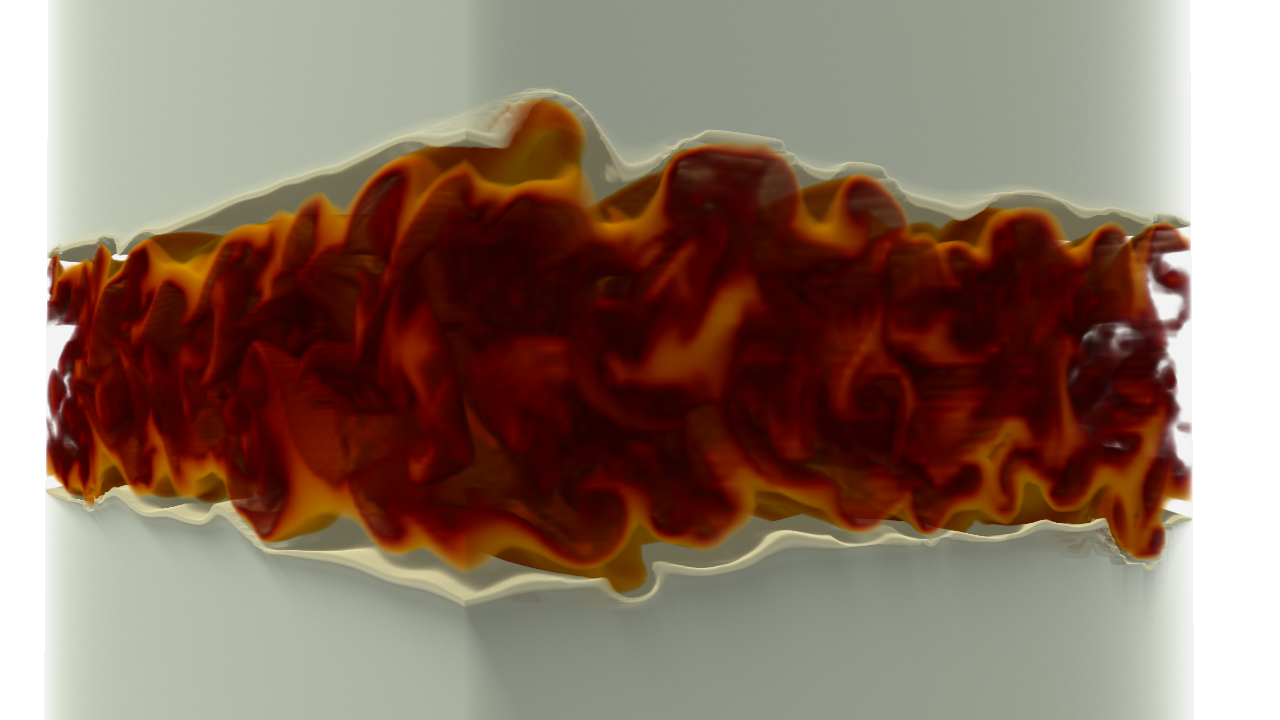
Figure 14: Volume renderings of a turbulent jet flame dataset. The original data at full resolution $[920\times 1400\times 72]$ is shown at the top. The middle row shows the reduced meshes obtained after ingesting 8 MB and 16 MB, respectively, using the by-coefficient-energy stream. The bottom row shows reduced meshes using the by-level-coeff stream. Both streams produce high quality visualizations, particularly after ingesting 16 MB.

References

- [1] J. Chen, A. Choudhary, S. Feldman, B. Hendrickson, C. R. Johnson, R. Mount, V. Sarkar, V. White, and D. Williams, Synergistic Challenges in Data-Intensive Science and Exascale Computing: DOE ASCAC Data Subcommittee Report, 2013.
- [2] D. E. Laney, S. Langer, C. Weber, P. Lindstrom, and A. Wegener, “Assessing the effects of data compression in simulations using physically motivated metrics,” in Int. Conf. for High Perf. Computing, Networking, Storage, and Analysis (SC), 2013, pp. 1–12.
- [3] J. Iverson, C. Kamath, and G. Karypis, “Fast and effective lossy compression algorithms for scientific datasets,” in European Conf. on Parallel Processing, 2012, pp. 843–856.
- [4] P. Lindstrom, “Fixed-rate compressed floating-point arrays,” IEEE Trans. on Vis. and Comp. Graph., vol. 20, no. 12, pp. 2674–2683, 2014.
- [5] R. Shekhar, E. Fayyad, R. Yagel, and J. F. Cornhill, “Octree-based decimation of marching cubes surfaces,” in Proc. of 7th Annual IEEE Vis., 1996, pp. 335–342.
- [6] V. Pascucci and R. Frank, “Global static indexing for real-time exploration of very large regular grids,” in Proc. of the 2001 ACM/IEEE Conf. on Supercomputing, 2001, pp. 45–45.
- [7] D. Hoang, P. Klacansky, H. Bhatia, P.-T. Bremer, P. Lindstrom, and V. Pascucci, “A study of the trade-off between reducing precision and reducing resolution for data analysis and visualization,” IEEE Trans. on Vis. and Comp. Graph., vol. 25, no. 1, pp. 1193–1203, 2019.
- [8] D. Hoang, B. Summa, H. Bhatia, P. Lindstrom, P. Klacansky, W. Usher, P.-T. Bremer, and V. Pascucci, “Efficient and flexible hierarchical data layouts for a unified encoding of scalar field precision and resolution,” IEEE Trans. on Vis. and Comp. Graph., vol. 27, no. 2, pp. 603–613, 2021.
- [9] W. Schroeder, K. Martin, and B. Lorensen, The Visualization Toolkit, 4th ed. Kitware, 2006.
- [10] J. Ahrens, B. Geveci, and C. Law, “ParaView: An end-user tool for large data visualization,” Visualization Handbook, 2005.
- [11] H. Childs, E. Brugger, B. Whitlock, J. Meredith, S. Ahern, D. Pugmire, K. Biagas, M. Miller, C. Harrison, G. H. Weber, H. Krishnan, T. Fogal, A. Sanderson, C. Garth, E. W. Bethel, D. Camp, O. Rübel, M. Durant, J. M. Favre, and P. Navrátil, “VisIt: An end-user tool for visualizing and analyzing very large data,” in High Performance Visualization–Enabling Extreme-Scale Scientific Insight, 2012.
- [12] N. Morrical, W. Usher, I. Wald, and V. Pascucci, “Efficient space skipping and adaptive sampling of unstructured volumes using hardware accelerated ray tracing,” in IEEE Vis. Conf. (VIS), 2019, pp. 256–260.
- [13] N. Morrical, I. Wald, W. Usher, and V. Pascucci, “Accelerating unstructured mesh point location with RT cores,” IEEE Trans. Vis. Comp. Graph., 2020.
- [14] I. Wald, G. P. Johnson, J. Amstutz, C. Brownlee, A. Knoll, J. Jeffers, J. Günther, and P. Navrátil, “OSPRay - A CPU Ray Tracing Framework for Scientific Visualization,” IEEE Trans. Vis. Comp. Graph., vol. 23, no. 1, pp. 931–940, 2017.
- [15] K. Weiss and P. Lindstrom, “Adaptive multilinear tensor product wavelets,” IEEE Trans. on Vis. and Comp. Graph., vol. 22, no. 1, pp. 985–994, 2016.
- [16] A. Cohen, I. Daubechies, and J.-C. Feauveau, “Biorthogonal bases of compactly supported wavelets,” Comm. on Pure and Appl. Math., vol. 45, no. 5, pp. 485–560, 1992.
- [17] T. Fogal, H. Childs, S. Shankar, J. Krüger, R. D. Bergeron, and P. Hatcher, “Large data visualization on distributed memory multi-GPU clusters,” in High Perf. Graph., 2010, p. 57–66.
- [18] J. Woodring, J. Ahrens, J. Figg, J. Wendelberger, S. Habib, and K. Heitmann, “In-situ sampling of a large-scale particle simulation for interactive visualization and analysis,” in Proc. of the 13th Eurographics Conf. on Vis., 2011, pp. 1151–1160.
- [19] C. L. Jackins and S. L. Tanimoto, “Oct-trees and their use in representing three-dimensional objects,” Comput. Graph. Image Process., vol. 14, no. 3, pp. 249–270, 1980.
- [20] C. Crassin, F. Neyret, S. Lefebvre, and E. Eisemann, “GigaVoxels: Ray-guided streaming for efficient and detailed voxel rendering,” in Proc. of the Symp. on Interactive 3D Graph. and Games, 2009, pp. 15–22.
- [21] E. Gobbetti, F. Marton, and J. A. Iglesias Guitián, “A single-pass gpu ray casting framework for interactive out-of-core rendering of massive volumetric datasets,” Vis. Comput., vol. 24, no. 7, pp. 797–806, 2008.
- [22] J. Beyer, M. Hadwiger, and H. Pfister, “State-of-the-art in GPU-based large-scale volume visualization,” Comp. Graph. Forum, vol. 34, no. 8, p. 13–37, 2015.
- [23] K. Museth, “VDB: High-resolution sparse volumes with dynamic topology,” ACM Trans. Graph., vol. 32, no. 3, 2013.
- [24] R. Setaluri, M. Aanjaneya, S. Bauer, and E. Sifakis, “SPGrid: A sparse paged grid structure applied to adaptive smoke simulation,” ACM Trans. Graph., vol. 33, no. 6, 2014.
- [25] M. Berger and P. Colella, “Local adaptive mesh refinement for shock hydrodynamics,” J. Comp. Phys., vol. 82, no. 1, pp. 64–84, 1989.
- [26] A. Dubey, A. Almgren, J. Bell, M. Berzins, S. Brandt, G. Bryan, P. Colella, D. Graves, M. Lijewski, F. Löffler, B. O’Shea, E. Schnetter, B. Van Straalen, and K. Weide, “A survey of high level frameworks in block-structured adaptive mesh refinement packages,” J. Parallel Distrib. Comput., vol. 74, no. 12, p. 3217–3227, 2014.
- [27] G. H. Weber, O. Kreylos, T. J. Ligocki, J. M. Shalf, H. Hagen, B. Hamann, and K. I. Joy, “Extraction of crack-free isosurfaces from adaptive mesh refinement data,” in Eurographics / IEEE VGTC Symp. on Visualization, 2001.
- [28] P. Moran and D. Ellsworth, “Visualization of AMR data with multi-level dual-mesh interpolation,” IEEE Trans. Vis. Comp. Graph., vol. 17, no. 12, pp. 1862–1871, 2011.
- [29] P. Ljung, C. F. Lundström, and A. Ynnerman, “Multiresolution interblock interpolation in direct volume rendering,” in Proc. of the Eighth Joint Eurographics / IEEE VGTC Conf. on Vis., 2006, pp. 259–266.
- [30] F. Wang, I. Wald, Q. Wu, W. Usher, and C. R. Johnson, “CPU isosurface ray tracing of adaptive mesh refinement data,” IEEE Trans. Vis. Comp. Graph., vol. 25, no. 1, pp. 1142–1151, 2019.
- [31] S. Li, S. Jaroszynski, S. Pearse, L. Orf, and J. Clyne, “Vapor: A visualization package tailored to analyze simulation data in earth system science,” Atmosphere, vol. 10, no. 9, 2019.
- [32] M. Treib, K. Bürger, F. Reichl, C. Meneveau, A. Szalay, and R. Westermann, “Turbulence visualization at the terascale on desktop pcs,” IEEE Trans. Vis. Comp. Graph., vol. 18, no. 12, pp. 2169–2177, 2012.
- [33] S. Li, S. Sane, L. Orf, P. Mininni, J. Clyne, and H. Childs, “Spatiotemporal wavelet compression for visualization of scientific simulation data,” in IEEE Int. Conf. on Cluster Computing, 2017, pp. 216–227.
- [34] J. Woodring, S. Mniszewski, C. Brislawn, D. DeMarle, and J. Ahrens, “Revisiting wavelet compression for large-scale climate data using jpeg 2000 and ensuring data precision,” in IEEE Symp. on Large Data Analysis and Vis., 2011, pp. 31–38.
- [35] M. Bertram, M. A. Duchaineau, B. Hamann, and K. I. Joy, “Generalized b-spline subdivision-surface wavelets for geometry compression,” IEEE Trans. Vis. Comp. Graph., vol. 10, no. 3, pp. 326–338, 2004.
- [36] M. H. Gross, O. G. Staadt, and R. Gatti, “Efficient triangular surface approximations using wavelets and quadtree data structures,” IEEE Trans. on Vis. and Comp. Graph., vol. 2, no. 2, pp. 130–143, 1996.
- [37] L. Linsen, V. Pascucci, M. Duchaineau, B. Hamann, and K. Joy, “Wavelet-based multiresolution with n-th-root-of-2,” in Dagstuhl Seminar on Geometric Modeling, 2004.
- [38] W. E. Lorensen and H. E. Cline, “Marching Cubes: A high resolution 3D surface construction algorithm,” SIGGRAPH Comput. Graph., vol. 21, no. 4, 1987.
- [39] P. Cignoni, F. Ganovelli, C. Montani, and R. Scopigno, “Reconstruction of topologically correct and adaptive trilinear isosurfaces,” Comput. Graph., vol. 24, no. 3, pp. 399–418, 2000.
- [40] G. M. Nielson, “On marching cubes,” IEEE Trans. Vis. Comp. Graph., vol. 9, no. 3, pp. 283–297, 2003.
- [41] M. Ament, D. Weiskopf, and H. Carr, “Direct interval volume visualization,” IEEE Trans. Vis. Comp. Graph., vol. 16, no. 6, pp. 1505–1514, 2010.
- [42] C. Zenger and W. Hackbusch, “Sparse grids,” in Research Workshop of the Israel Science Foundation on Multiscale Phenomenon, Modelling and Computation, 1991, p. 86.
- [43] J. Garcke, “Sparse grids in a nutshell,” in Sparse grids and applications. Springer, 2012, pp. 57–80.
- [44] D. Tao, S. Di, Z. Chen, and F. Cappello, “Significantly improving lossy compression for scientific data sets based on multidimensional prediction and error-controlled quantization,” in IEEE Int. Par. and Dist. Process. Symp., 2017, pp. 1129–1139.
- [45] R. Ballester-Ripoll, P. Lindstrom, and R. Pajarola, “TTHRESH: Tensor compression for multidimensional visual data,” IEEE Trans. on Vis. and Comp. Graph., vol. 26, no. 9, pp. 2891–2903, 2020.
- [46] M. Ainsworth, O. Tugluk, B. Whitney, and S. Klasky, “Multilevel techniques for compression and reduction of scientific data–the univariate case,” Comput. Vis. Sci., vol. 19, no. 5-6, pp. 65–76, 2018.
- [47] ——, “Multilevel techniques for compression and reduction of scientific data—the multivariate case,” SIAM Journal on Scientific Computing, vol. 41, no. 2, pp. A1278–A1303, 2019.
- [48] K. Zhao, S. Di, M. Dmitriev, T.-L. D. Tonellot, Z. Chen, and F. Cappello, “Optimizing error-bounded lossy compression for scientific data by dynamic spline interpolation,” in IEEE 37th Int. Conf. on Data Eng., 2021, pp. 1643–1654.
- [49] C. Chrysafis, A. Said, A. Drukarev, A. Islam, and W. Pearlman, “Sbhp-a low complexity wavelet coder,” in IEEE Int. Conf. on Acoustics, Speech, and Signal Processing, vol. 4, 2000, pp. 2035–2038.
- [50] W. Pearlman, A. Islam, N. Nagaraj, and A. Said, “Efficient, low-complexity image coding with a set-partitioning embedded block coder,” IEEE Trans. Circuits Sys. Video Tech., vol. 14, no. 11, pp. 1219–1235, 2004.
- [51] A. Said and W. Pearlman, “A new, fast, and efficient image codec based on set partitioning in hierarchical trees,” IEEE Trans. Circuits Sys. Video Tech., vol. 6, no. 3, pp. 243–250, 1996.
- [52] A. Skodras, C. Christopoulos, and T. Ebrahimi, “The JPEG 2000 still image compression standard,” IEEE Signal Process. Mag., vol. 18, no. 5, pp. 36–58, 2001.
- [53] S. Li, S. Jaroszynski, S. Pearse, L. Orf, and J. Clyne, “Vapor: A visualization package tailored to analyze simulation data in earth system science,” Atmosphere, vol. 10, no. 9, p. 488, 2019.
- [54] S. Mallat, A wavelet tour of signal processing. Academic Press, 2008.
- [55] S. F. Frisken and R. N. Perry, “Simple and efficient traversal methods for quadtrees and octrees,” J. Graphics Tools, vol. 7, no. 3, pp. 1–11, 2002.
- [56] I. Gargantini, “An effective way to represent quadtrees,” Commun. ACM, vol. 25, no. 12, 1982.
- [57] K. Museth, “Nanovdb: A gpu-friendly and portable vdb data structure for real-time rendering and simulation,” in ACM SIGGRAPH Talks, 2021.
- [58] F. Guo, H. Li, W. Daughton, and Y.-H. Liu, “Formation of hard power laws in the energetic particle spectra resulting from relativistic magnetic reconnection,” Phys. Rev. Lett., vol. 113, 2014.
- [59] R. H. Cohen, W. P. Dannevik, A. M. Dimits, D. E. Eliason, A. A. Mirin, Y. Zhou, D. H. Porter, and P. R. Woodward, “Three-dimensional simulation of a richtmyer–meshkov instability with a two-scale initial perturbation,” Phys. of Fluids, vol. 14, no. 10, pp. 3692–3709, 2002.
- [60] W. H. Cabot and A. W. Cook, “Reynolds number effects on Rayleigh–Taylor instability with possible implications for type Ia supernovae,” Nature Phys., vol. 2, pp. 562–568, 2006.