The magnetic moment of $Z_{c}(3900)$ as an axial-vector molecular state

Yong-Jiang Xu1111xuyongjiang13@nudt.edu.cn, Yong-Lu Liu1, and Ming-Qiu Huang1,2222corresponding author: mqhuang@nudt.edu.cn 1Department of Physics, College of Liberal Arts and Sciences, National University of Defense Technology , Changsha, 410073, Hunan, China 2Synergetic Innovation Center for Quantum Effects and Applications, Hunan Normal University, Changsha, 410081, Hunan, China
Abstract

In this paper, we tentatively assign $Z_{c}(3900)$ to be an axialvector molecular state, and calculate its magnetic moment using the QCD sum rule method in external weak electromagnetic field. Starting with the two-point correlation function in external electromagnetic field and expanding it in power of the electromagnetic interaction Hamiltonian, we extract the mass and pole residue of $Z_{c}(3900)$ state from the leading term in the expansion and the magnetic moment from the linear response to the external electromagnetic field. The numerical values are $m_{Z_{c}}=3.97\pm 0.12\mbox{GeV}$ in agreement with the experimental value $m^{exp}_{Z_{c}}=3899.0\pm 3.6\pm 4.9\mbox{MeV}$, $\lambda_{Z_{c}}=2.1\pm 0.4\times 10^{-2}\mbox{GeV}^{5}$ and $\mu_{Z_{c}}=0.19^{+0.04}_{-0.01}\mu_{N}$.

pacs:
11.25.Hf,Β  11.55.Hx,Β  12.38.Lg,Β  12.39.Mk.

I Introduction

$Z_{c}(3900)$, as a good candidate of exotic hadrons, was observed by BESIII collaboration in 2013 in the $\pi^{\pm}J/\psi$ invariant mass distribution of the process $e^{+}e^{-}\rightarrow\pi^{+}\pi^{-}J/\psi$ at a center-of-mass energy of $4.260\mbox{GeV}$ bes1 . Then the Belle and CLEO collaborations confirmed the existence of $Z_{c}(3900)$ belle ; cleo . In 2017, the BESIII collaboration determined the $J^{P}$ quantum number of $Z_{c}(3900)$ to be $J^{P}=1^{+}$ with a statistical significance larger than $7\sigma$ over other quantum numbers in a partial wave analysis of the process $e^{+}e^{-}\rightarrow\pi^{+}\pi^{-}J/\psi$ bes2 . Inspired by these experimental progress, there have been plentiful theoretical studies on $Z_{c}(3900)$’s properties through different approaches (see review article H.X.Chen and references therein for details). However, the underlying structure of $Z_{c}(3900)$ is not understood completely and more endeavors are necessary in order to arrive at a better understanding for the properties of $Z_{c}(3900)$.

The electromagnetic multipole moments of hadron encode the spatial distributions of charge and magnetization in the hadron and provide important information about the quark configurations of the hadron and the underlying dynamics. So it is interesting to study the electromagnetic multipole moments of hadron.

The studies on the properties of hadrons inevitably involve the nonperturbative effects of quantum chromodynamics (QCD). The QCD sum rule method SVZ is a nonperturbative analytic formalism firmly entrenched in QCD with minimal modeling and has been successfully applied in almost every aspect of strong interaction physics. In Ref.Balitsky ; Ioffe1 ; Ioffe2 , the QCD sum rule method was extended to calculate the magnetic moments of the nucleon and hyperon in the external field method. In this method, a statics electromagnetic field is introduced which couples to the quarks and polarizes the QCD vacuum and magnetic moments can be extracted from the linear response to this field. Later, a more systematic studies was made for the magnetic moments of the octet baryons octet1 ; octet2 ; octet3 ; octet4 , the decuplet baryons decuplet1 ; decuplet2 ; decuplet3 ; decuplet4 and the $\rho$ meson rho . In the case of the exotic X, Y, Z states, only the magnetic moment of $Z_{c}(3900)$ as an axialvector tetraquark state was calculated through this method wangzhigang .

In this article, we study the magnetic moment of $Z_{c}(3900)$ as an axialvector molecular state with quantum number $J^{P}=1^{+}$ by the QCD sum rule method. The mass and pole residue, two of the input parameters needed to determine the magnetic moment, are calculated firstly including contributions of operators up to dimension 10. Then the magnetic moment is extracted from the linear term in $F_{\mu\nu}$ (external electromagnetic filed) of the correlation function.

The rest of the paper is arranged as follows. In Sec.II, we derive the sum rules for the mass, pole residue and magnetic moment of $Z_{c}(3900)$ state. Sec.III is devoted to the numerical analysis and a short summary is given in Sec.IV. In the Appendix B, the spectral densities are shown.

II The derivation of the sum rules

The starting point of our calculation is the time-ordered correlation function in the QCD vacuum in the presence of a constant background electromagnetic field $F_{\mu\nu}$,

Πμ​ν​(p)=iβ€‹βˆ«π‘‘x4​ei​p​xβ€‹βŸ¨0∣T​[Jμ​(x)​Jν†​(0)]∣0⟩F=Πμ​ν(0)​(p)+Πμ​ν​α​β(1)​(p)​Fα​β+β‹―,subscriptΞ πœ‡πœˆπ‘π‘–differential-dsuperscriptπ‘₯4superscript𝑒𝑖𝑝π‘₯subscriptquantum-operator-product0Tdelimited-[]subscriptπ½πœ‡π‘₯subscriptsuperscriptπ½β€ πœˆ00𝐹subscriptsuperscriptΞ 0πœ‡πœˆπ‘subscriptsuperscriptΞ 1πœ‡πœˆπ›Όπ›½π‘superscript𝐹𝛼𝛽⋯\Pi_{\mu\nu}(p)=i\int dx^{4}e^{ipx}\langle 0\mid\textsl{T}[J_{\mu}(x)J^{\dagger}_{\nu}(0)]\mid 0\rangle_{F}=\Pi^{(0)}_{\mu\nu}(p)+\Pi^{(1)}_{\mu\nu\alpha\beta}(p)F^{\alpha\beta}+\cdots, (1)

where

$$J_{\mu}(x)=\frac{1}{\sqrt{2}}\{[\bar{u}(x)i\gamma^{5}c(x)][\bar{c}(x)\gamma_{\mu}d(x)]+[\bar{u}(x)\gamma_{\mu}c(x)][\bar{c}(x)i\gamma^{5}d(x)]\}$$ (2)

is the interpolating current of $Z_{c}(3900)$ as a molecular state with $J^{P}=1^{+}$ cuichunyu . The Πμ​ν(0)​(p)subscriptsuperscriptΞ 0πœ‡πœˆπ‘\Pi^{(0)}_{\mu\nu}(p) term is the correlation function without external electromagnetic field, and give rise to the mass and pole residue of $Z_{c}(3900)$. The magnetic moment will be extracted from the linear response term, Πμ​ν​α​β(1)​(p)​Fα​βsubscriptsuperscriptΞ 1πœ‡πœˆπ›Όπ›½π‘superscript𝐹𝛼𝛽\Pi^{(1)}_{\mu\nu\alpha\beta}(p)F^{\alpha\beta}.

The external electromagnetic field can interact directly with the quarks inside the hadron and also polarize the QCD vacuum. As a consequence, the vacuum condensates involved in the operator product expansion of the correlation function in the external electromagnetic field $F_{\mu\nu}$ are,

  • β€’

    dimension-2 operator,

    $$F_{\mu\nu},$$ (3)
  • β€’

    dimension-3 operator,

    $$\langle 0|\bar{q}\sigma_{\mu\nu}q|0\rangle_{F},$$ (4)
  • β€’

    dimension-5 operators,

    $$\langle 0|\bar{q}q|0\rangle F_{\mu\nu},\langle 0|\bar{q}g_{s}G_{\mu\nu}q|0\rangle_{F},\epsilon_{\mu\nu\alpha\beta}\langle 0|\bar{q}g_{s}G^{\alpha\beta}q|0\rangle_{F},$$ (5)
  • β€’

    dimension-6 operators,

    $$\langle 0|\bar{q}q|0\rangle\langle 0|\bar{q}\sigma_{\mu\nu}q|0\rangle_{F},\langle 0|g^{2}_{s}GG|0\rangle F_{\mu\nu},\cdots,$$ (6)
  • β€’

    dimension-7 operators,

    ⟨0|gs2​G​G|0βŸ©β€‹βŸ¨0|q¯​σμ​ν​q|0⟩F,⟨0|gs​q¯​σ⋅G​q|0βŸ©β€‹Fμ​ν,β‹―,quantum-operator-product0subscriptsuperscript𝑔2𝑠𝐺𝐺0subscriptquantum-operator-product0Β―π‘žsubscriptπœŽπœ‡πœˆπ‘ž0𝐹quantum-operator-product0β‹…subscriptπ‘”π‘ Β―π‘žπœŽπΊπ‘ž0subscriptπΉπœ‡πœˆβ‹―\langle 0|g^{2}_{s}GG|0\rangle\langle 0|\bar{q}\sigma_{\mu\nu}q|0\rangle_{F},\langle 0|g_{s}\bar{q}\sigma\cdot Gq|0\rangle F_{\mu\nu},\cdots, (7)
  • β€’

    dimension-8 operators,

    ⟨0|q¯​q|0⟩2​Fμ​ν,⟨0|gs​q¯​σ⋅G​q|0βŸ©β€‹βŸ¨0|q¯​σμ​ν​q|0⟩F,⟨0|q¯​q|0βŸ©β€‹βŸ¨0|q¯​gs​Gμ​ν​q|0⟩F,superscriptquantum-operator-product0Β―π‘žπ‘ž02subscriptπΉπœ‡πœˆquantum-operator-product0β‹…subscriptπ‘”π‘ Β―π‘žπœŽπΊπ‘ž0subscriptquantum-operator-product0Β―π‘žsubscriptπœŽπœ‡πœˆπ‘ž0𝐹quantum-operator-product0Β―π‘žπ‘ž0subscriptquantum-operator-product0Β―π‘žsubscript𝑔𝑠subscriptπΊπœ‡πœˆπ‘ž0𝐹\displaystyle\langle 0|\bar{q}q|0\rangle^{2}F_{\mu\nu},\langle 0|g_{s}\bar{q}\sigma\cdot Gq|0\rangle\langle 0|\bar{q}\sigma_{\mu\nu}q|0\rangle_{F},\langle 0|\bar{q}q|0\rangle\langle 0|\bar{q}g_{s}G_{\mu\nu}q|0\rangle_{F},
    $\displaystyle\epsilon_{\mu\nu\alpha\beta}\langle 0|\bar{q}q|0\rangle\langle 0|\bar{q}g_{s}G^{\alpha\beta}q|0\rangle_{F},\cdots,$ (8)

The new vacuum condensates induced by the external electromagnetic field $F_{\mu\nu}$ can be described by introducing new parameters, $\chi$, $\kappa$ and $\xi$, called vacuum susceptibilities as follows,

$\displaystyle\langle 0|\bar{q}\sigma_{\mu\nu}q|0\rangle_{F}=ee_{q}\chi\langle 0|\bar{q}q|0\rangle F_{\mu\nu},$
$\displaystyle\langle 0|\bar{q}g_{s}G_{\mu\nu}q|0\rangle_{F}=ee_{q}\kappa\langle 0|\bar{q}q|0\rangle F_{\mu\nu},$
$\displaystyle\epsilon_{\mu\nu\alpha\beta}\langle 0|\bar{q}g_{s}G^{\alpha\beta}q|0\rangle_{F}=iee_{q}\xi\langle 0|\bar{q}q|0\rangle F_{\mu\nu}.$ (9)

In order to express the two-point correlation function (1) physically, we expand it in powers of the electromagnetic interaction Hamiltonian $H_{int}=-ie\int d^{4}yj^{em}_{\alpha}(y)A^{\alpha}(y)$,

Πμ​ν​(p)=subscriptΞ πœ‡πœˆπ‘absent\displaystyle\Pi_{\mu\nu}(p)= iβ€‹βˆ«π‘‘x4​ei​p​xβ€‹βŸ¨0∣T​[Jμ​(x)​Jν†​(0)]∣0βŸ©π‘–differential-dsuperscriptπ‘₯4superscript𝑒𝑖𝑝π‘₯quantum-operator-product0Tdelimited-[]subscriptπ½πœ‡π‘₯subscriptsuperscriptπ½β€ πœˆ00\displaystyle i\int dx^{4}e^{ipx}\langle 0\mid\textsl{T}[J_{\mu}(x)J^{\dagger}_{\nu}(0)]\mid 0\rangle (10)
+iβ€‹βˆ«π‘‘x4​ei​p​xβ€‹βŸ¨0∣T​{Jμ​(x)​[βˆ’i​eβ€‹βˆ«d4​y​jΞ±e​m​(y)​Aα​(y)]​Jν†​(0)}∣0⟩+β‹―,𝑖differential-dsuperscriptπ‘₯4superscript𝑒𝑖𝑝π‘₯quantum-operator-product0Tsubscriptπ½πœ‡π‘₯delimited-[]𝑖𝑒superscript𝑑4𝑦subscriptsuperscriptπ‘—π‘’π‘šπ›Όπ‘¦superscript𝐴𝛼𝑦subscriptsuperscriptπ½β€ πœˆ00β‹―\displaystyle+i\int dx^{4}e^{ipx}\langle 0\mid\textsl{T}\{J_{\mu}(x)[-ie\int d^{4}yj^{em}_{\alpha}(y)A^{\alpha}(y)]J^{\dagger}_{\nu}(0)\}\mid 0\rangle+\cdots,

where $j^{em}_{\alpha}(y)$ is the electromagnetic current and $A^{\alpha}(y)$ is the electromagnetic four-vector.

Inserting complete sets of relevant states with the same quantum numbers as the current operator $J_{\mu}(x)$ and carrying out involved integrations, one has

Πμ​νh​a​d​(p)=subscriptsuperscriptΞ β„Žπ‘Žπ‘‘πœ‡πœˆπ‘absent\displaystyle\Pi^{had}_{\mu\nu}(p)= $\displaystyle\frac{\lambda^{2}_{Z_{c}}}{m^{2}_{Z_{c}}-p^{2}}(-g_{\mu\nu}+\frac{p_{\mu}p_{\nu}}{p^{2}})$ (11)
$\displaystyle-i\frac{\lambda^{2}_{Z_{c}}G_{2}(0)}{(p^{2}-m^{2}_{Z_{c}})^{2}}F_{\mu\nu}+i\frac{a}{m^{2}_{Z_{c}}-p^{2}}F_{\mu\nu}+\cdots,$

where we make use of the following matrix elements

$$\langle 0|J_{\mu}(0)|Z_{c}(p)\rangle=\lambda_{Z_{c}}\epsilon_{\mu}(p)$$ (12)

with $\lambda_{Z_{c}}$ and $\epsilon_{\mu}(p)$ being the pole residue and polarization vector of $Z_{c}(3900)$, respectively,

$\displaystyle\langle Z_{c}(p)|j^{em}_{\alpha}(0)|Z_{c}(p^{\prime})\rangle=$ $\displaystyle G_{1}(Q^{2})\epsilon^{*}(p)\cdot\epsilon(p^{\prime})(p+p^{\prime})_{\alpha}+G_{2}(Q^{2})[\epsilon_{\alpha}(p^{\prime})\epsilon^{*}(p)\cdot q-\epsilon^{*}_{\alpha}(p)\epsilon(p^{\prime})\cdot q]$ (13)
$\displaystyle-\frac{G_{3}(Q^{2})}{2m^{2}_{Z_{c}}}\epsilon^{*}(p)\cdot q\epsilon(p^{\prime})\cdot q(p+p^{\prime})_{\alpha}$

with $q=p^{\prime}-p$ and $Q^{2}=-q^{2}$. The Lorentz-invariant functions $G_{1}(Q^{2})$, $G_{2}(Q^{2})$ and $G_{3}(Q^{2})$ are related to the charge, magnetic and quadrupole form-factors,

$\displaystyle G_{C}(Q^{2})=G_{1}(Q^{2})+\frac{2}{3}\eta G_{Q}(Q^{2}),$
$\displaystyle G_{M}(Q^{2})=-G_{2}(Q^{2}),$
$\displaystyle G_{Q}(Q^{2})=G_{1}(Q^{2})+G_{2}(Q^{2})+(1+\eta)G_{3}(Q^{2}),$ (14)

respective, where $\eta=\frac{Q^{2}}{4m^{2}_{Z_{c}}}$. At zero momentum transfer, these form-factors are proportional to the usual static quantities of the charge $e$, magnetic moment $\mu_{Z_{c}}$ and quadrupole moment $Q_{1}$,

$\displaystyle eG_{C}(0)=e,$
$\displaystyle eG_{M}(0)=2m_{Z}\mu_{Z_{c}},$
$\displaystyle eG_{Q}(0)=m^{2}_{Z_{c}}Q_{1}.$ (15)

The constant $a$ parameterizes the contributions from the pole-continuum transitions.

On the other hand, Πμ​ν​(p)subscriptΞ πœ‡πœˆπ‘\Pi_{\mu\nu}(p) can be calculated theoretically via OPE method at the quark-gluon level. To this end, one can insert the interpolating current $J_{\mu}(x)$ (2) into the correlation function (1), contract the relevant quark fields via Wick’s theorem and obtain

Πμ​νO​P​E​(p)=i2β€‹βˆ«d4​x​ei​p​xsubscriptsuperscriptΞ π‘‚π‘ƒπΈπœ‡πœˆπ‘π‘–2superscript𝑑4π‘₯superscript𝑒𝑖𝑝π‘₯\displaystyle\Pi^{OPE}_{\mu\nu}(p)=\frac{i}{2}\int d^{4}xe^{ipx} $\displaystyle(Tr[(i\gamma_{5})S^{(u)}_{ca}(-x)(i\gamma_{5})S^{(c)}_{ac}(x)]Tr[\gamma_{\mu}S^{(d)}_{bd}(x)\gamma_{\nu}S^{(c)}_{db}(-x)]$ (16)
$\displaystyle+Tr[(i\gamma_{5})S^{(c)}_{db}(-x)\gamma_{\mu}S^{(d)}_{bd}(x)]Tr[(i\gamma_{5})S^{(c)}_{ac}(x)\gamma_{\nu}S^{(u)}_{ca}(-x)]$
$\displaystyle+Tr[(i\gamma_{5})S^{(u)}_{ca}(-x)\gamma_{\mu}S^{(c)}_{ac}(x)]Tr[(i\gamma_{5})S^{(d)}_{bd}(x)\gamma_{\nu}S^{(c)}_{db}(-x)]$
$\displaystyle+Tr[(i\gamma_{5})S^{(d)}_{bd}(x)(i\gamma_{5})S^{(c)}_{db}(-x)]Tr[\gamma_{\mu}S^{(c)}_{ac}(x)\gamma_{\nu}S^{(u)}_{ca}(-x)]),$

where $S^{(c)}(x)=\langle 0|T[c(x)\bar{c}(0)]|0\rangle$ and $S^{(q)}(x)=\langle 0|T[q(x)\bar{q}(0)]|0\rangle,q=u,d$ are the full charm- and up (down)-quark propagators, whose expressions are given in the Appendix A, $Tr$ denotes the trace of the Dirac spinor indices, and $a$, $b$, $c$ and $d$ are color indices. Through dispersion relation, Πμ​νO​P​E​(p)subscriptsuperscriptΞ π‘‚π‘ƒπΈπœ‡πœˆπ‘\Pi^{OPE}_{\mu\nu}(p) can be written as

Πμ​νO​P​E​(p)=∫4​mc2βˆžπ‘‘s​ρ(0)​(s)sβˆ’p2​(βˆ’gμ​ν+pμ​pΞ½p2)+∫4​mc2βˆžπ‘‘s​ρ(1)​(s)sβˆ’p2​(i​Fμ​ν)+other Lorentz structures,subscriptsuperscriptΞ π‘‚π‘ƒπΈπœ‡πœˆπ‘subscriptsuperscript4subscriptsuperscriptπ‘š2𝑐differential-d𝑠superscript𝜌0𝑠𝑠superscript𝑝2subscriptπ‘”πœ‡πœˆsubscriptπ‘πœ‡subscriptπ‘πœˆsuperscript𝑝2subscriptsuperscript4subscriptsuperscriptπ‘š2𝑐differential-d𝑠superscript𝜌1𝑠𝑠superscript𝑝2𝑖subscriptπΉπœ‡πœˆother Lorentz structures\Pi^{OPE}_{\mu\nu}(p)=\int^{\infty}_{4m^{2}_{c}}ds\frac{\rho^{(0)}(s)}{s-p^{2}}(-g_{\mu\nu}+\frac{p_{\mu}p_{\nu}}{p^{2}})+\int^{\infty}_{4m^{2}_{c}}ds\frac{\rho^{(1)}(s)}{s-p^{2}}(iF_{\mu\nu})+\mbox{other Lorentz structures}, (17)

where ρi​(s)=1π​Im​ΠiO​P​E​(s),i=0,1formulae-sequencesuperscriptπœŒπ‘–π‘ 1πœ‹ImsubscriptsuperscriptΠ𝑂𝑃𝐸𝑖𝑠𝑖01\rho^{i}(s)=\frac{1}{\pi}\mbox{Im}\Pi^{OPE}_{i}(s),i=0,1 are the spectral densities. The spectral densities ρi​(s)superscriptπœŒπ‘–π‘ \rho^{i}(s) are given in the Appendix B.

Finally, matching the phenomenological side (11) and the QCD representation (17), we obtain

$$\frac{\lambda^{2}_{Z_{c}}}{m^{2}_{Z_{c}}-p^{2}}+\cdots=\int^{\infty}_{4m^{2}_{c}}ds\frac{\rho^{(0)}(s)}{s-p^{2}},$$ (18)

for the Lorentz-structure $(-g_{\mu\nu}+\frac{p_{\mu}p_{\nu}}{p^{2}})$, and

$$\frac{\lambda^{2}_{Z_{c}}G_{M}(0)}{(m^{2}_{Z_{c}}-p^{2})^{2}}+\frac{a}{m^{2}_{Z_{c}}-p^{2}}+\cdots=\int^{\infty}_{4m^{2}_{c}}ds\frac{\rho^{(1)}(s)}{s-p^{2}},$$ (19)

for the Lorentz-structure $iF_{\mu\nu}$.

According to quark-hadron duality, the excited and continuum states’ spectral density can be approximated by the QCD spectral density above some effective threshold $s^{0}_{Z_{c}}$, whose vale will be determined in Sec.III,

$\displaystyle\frac{\lambda^{2}_{Z_{c}}}{m^{2}_{Z_{c}}-p^{2}}+\int^{\infty}_{s^{0}_{Z_{c}}}ds\frac{\rho^{(0)}(s)}{s-p^{2}}=\int^{\infty}_{4m^{2}_{c}}ds\frac{\rho^{(0)}(s)}{s-p^{2}},$
$\displaystyle\frac{\lambda^{2}_{Z_{c}}G_{M}(0)}{(m^{2}_{Z_{c}}-p^{2})^{2}}+\frac{a}{m^{2}_{Z_{c}}-p^{2}}+\int^{\infty}_{s^{0}_{Z_{c}}}ds\frac{\rho^{(1)}(s)}{s-p^{2}}=\int^{\infty}_{4m^{2}_{c}}ds\frac{\rho^{(1)}(s)}{s-p^{2}}.$ (20)

Subtracting the contributions of the excited and continuum states, one gets

$\displaystyle\frac{\lambda^{2}_{Z_{c}}}{m^{2}_{Z_{c}}-p^{2}}=\int^{s^{0}_{Z_{c}}}_{4m^{2}_{c}}ds\frac{\rho^{(0)}(s)}{s-p^{2}},$
$\displaystyle\frac{\lambda^{2}_{Z_{c}}G_{M}(0)}{(m^{2}_{Z_{c}}-p^{2})^{2}}+\frac{a}{m^{2}_{Z_{c}}-p^{2}}=\int^{s^{0}_{Z_{c}}}_{4m^{2}_{c}}ds\frac{\rho^{(1)}(s)}{s-p^{2}}.$ (21)

In order to improve the convergence of the OPE series and suppress the contributions from the excited and continuum states, it is necessary to make a Borel transform. As a result, we have

$\displaystyle\lambda^{2}_{Z_{c}}e^{-m^{2}_{Z_{c}}/M^{2}_{B}}=\int^{s^{0}_{Z_{c}}}_{4m^{2}_{c}}ds\rho^{(0)}(s)e^{-s/M^{2}_{B}},$
$\displaystyle\lambda^{2}_{Z_{c}}(\frac{G_{M}(0)}{M^{2}_{B}}+A)e^{-m^{2}_{Z_{c}}/M^{2}_{B}}=\int^{s^{0}_{Z_{c}}}_{4m^{2}_{c}}ds\rho^{(1)}(s)e^{-s/M^{2}_{B}}.$ (22)

where $M^{2}_{B}$ is the Borel parameter and $A=\frac{a}{\lambda^{2}_{Z_{c}}}$. Taking derivative of the first equation in (II) with respect to $-\frac{1}{M^{2}_{B}}$ and dividing it by the original expression, one has

$$m^{2}_{Z_{c}}=\frac{\frac{d}{d(-\frac{1}{M^{2}_{B}})}\int^{s^{0}_{Z_{c}}}_{4m^{2}_{c}}ds\rho^{(0)}(s)e^{-\frac{s}{M^{2}_{B}}}}{\int^{s^{0}_{Z_{c}}}_{4m^{2}_{c}}ds\rho^{(0)}(s)e^{-\frac{s}{M^{2}_{B}}}},$$ (23)

In the next section, (II) and (23) will be analysed numerically to obtain the numerical values of the mass, the pole residue and the magnetic moment of the $Z_{c}(3900)$.

III Numerical analysis

The input parameters needed in numerical analysis are presented in Table 1. For the vacuum susceptibilities $\chi$, $\kappa$ and $\xi$, we take the values $\chi=-(3.15\pm 0.30)\mbox{GeV}^{-2}$, $\kappa=-0.2$ and $\xi=0.4$ determined in the detailed QCD sum rules analysis of the photon light-cone distribution amplitudes P.Ball . Besides these parameters, we should determine the working intervals of the threshold parameter $s^{0}_{Z_{c}}$ and the Borel mass $M^{2}_{B}$ in which the mass, the pole residue and the magnetic moment vary weakly. The continuum threshold is related to the square of the first exited states having the same quantum number as the interpolating field, while the Borel parameter is determined by demanding that both the contributions of the higher states and continuum are sufficiently suppressed and the contributions coming from higher dimensional operators are small.

Table 1: Some input parameters needed in the calculations.
Parameter Value
$\langle\bar{q}q\rangle$ $-(0.24\pm 0.01)^{3}\mbox{GeV}^{3}$
⟨gs​q¯​σ​G​q⟩delimited-⟨⟩subscriptπ‘”π‘ Β―π‘žπœŽπΊπ‘ž\langle g_{s}\bar{q}\sigma Gq\rangle $(0.8\pm 0.1)\langle\bar{q}q\rangle\mbox{GeV}^{2}$
$\langle g^{2}_{s}GG\rangle$ $0.88\pm 0.25\mbox{GeV}^{4}$
$m_{c}$ $1.275^{+0.025}_{-0.035}\mbox{GeV}$M.Tanabashi

We define two quantities, the ratio of the pole contribution to the total contribution (RP) and the ratio of the highest dimensional term in the OPE series to the total OPE series (RH), as followings,

R​Piβ‰‘βˆ«4​mc2sZc0𝑑s​ρ(i)​(s)​eβˆ’sMB2∫4​mc2βˆžπ‘‘s​ρ(i)​(s)​eβˆ’sMB2,𝑅subscript𝑃𝑖subscriptsuperscriptsubscriptsuperscript𝑠0subscript𝑍𝑐4subscriptsuperscriptπ‘š2𝑐differential-d𝑠superscriptπœŒπ‘–π‘ superscript𝑒𝑠subscriptsuperscript𝑀2𝐡subscriptsuperscript4subscriptsuperscriptπ‘š2𝑐differential-d𝑠superscriptπœŒπ‘–π‘ superscript𝑒𝑠subscriptsuperscript𝑀2𝐡\displaystyle RP_{i}\equiv\frac{\int^{s^{0}_{Z_{c}}}_{4m^{2}_{c}}ds\rho^{(i)}(s)e^{-\frac{s}{M^{2}_{B}}}}{\int^{\infty}_{4m^{2}_{c}}ds\rho^{(i)}(s)e^{-\frac{s}{M^{2}_{B}}}},
R​Hiβ‰‘βˆ«4​mc2sZc0𝑑s​ρi(d=n)​(s)​eβˆ’sMB2∫4​mc2sZc0𝑑s​ρ(i)​(s)​eβˆ’sMB2,𝑅subscript𝐻𝑖subscriptsuperscriptsubscriptsuperscript𝑠0subscript𝑍𝑐4subscriptsuperscriptπ‘š2𝑐differential-d𝑠subscriptsuperscriptπœŒπ‘‘π‘›π‘–π‘ superscript𝑒𝑠subscriptsuperscript𝑀2𝐡subscriptsuperscriptsubscriptsuperscript𝑠0subscript𝑍𝑐4subscriptsuperscriptπ‘š2𝑐differential-d𝑠superscriptπœŒπ‘–π‘ superscript𝑒𝑠subscriptsuperscript𝑀2𝐡\displaystyle RH_{i}\equiv\frac{\int^{s^{0}_{Z_{c}}}_{4m^{2}_{c}}ds\rho^{(d=n)}_{i}(s)e^{-\frac{s}{M^{2}_{B}}}}{\int^{s^{0}_{Z_{c}}}_{4m^{2}_{c}}ds\rho^{(i)}(s)e^{-\frac{s}{M^{2}_{B}}}}, (24)

where $i=0,1$ and $n=10(8)$ as $i=0(1)$, respectively.

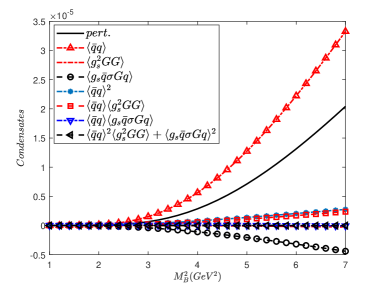
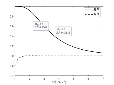
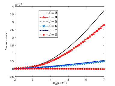
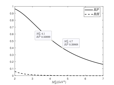
In Fig.1(a), we compare the various terms in the OPE series as functions of $M^{2}_{B}$ with $\sqrt{s^{0}_{Z_{c}}}=4.6\mbox{GeV}$. From it one can see that except the quark condensate $\langle\bar{q}q\rangle$, other vacuum condensates are much smaller than the perturbative term. So the OPE series are under control. Fig.1(b) shows $RP_{0}$ and $RH_{0}$ varying with $M^{2}_{B}$ at $\sqrt{s^{0}_{Z_{c}}}=4.6\mbox{GeV}$. The figure shows that the requirement $RP_{0}\geq 50\%$ ($RP_{0}\geq 40\%$) gives $M^{2}_{B}\leq 3.3\mbox{GeV}^{2}$ ($M^{2}_{B}\leq 3.7\mbox{GeV}^{2}$) and $RH_{0}=5\%$ at $M^{2}_{B}=1.25\mbox{GeV}^{2}$.

Refer to caption
Refer to caption
Figure 1: (a) denotes the various condensates as functions of $M^{2}_{B}$ with $\sqrt{s^{0}_{Z_{c}}}=4.6\mbox{GeV}$; (b) represents $RP_{0}$ and $RH_{0}$ varying with $M^{2}_{B}$ at $\sqrt{s^{0}_{Z_{c}}}=4.6\mbox{GeV}$.

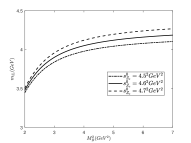
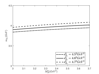
From Fig.2(a), we know that the sum rule for the mass $m_{Z_{c}}$ depends strongly on the Borel parameter $M^{2}_{B}$ as $M^{2}_{B}\leq 3\mbox{GeV}^{2}$. Along with the criterions of pole dominance, this fact confines $M^{2}_{B}$ from $3\mbox{GeV}^{2}$ to $3.7\mbox{GeV}^{2}$. In the analysis, we take $RP_{0}\geq 40\%$ so that we can obtain a larger interval of the Borel parameter. Within the interval of $M^{2}_{B}$ determined above, the mass varies weakly with $M^{2}_{B}$ as depicted in Fig.2(b). Fig.2(b) also shows the weak dependence of the mass on the threshold parameter $s^{0}_{Z_{c}}$ as $4.5^{2}\mbox{GeV}^{2}\leq s^{0}_{Z_{c}}\leq 4.7^{2}\mbox{GeV}^{2}$. As a result, we can reliably read the value of the mass, $m_{Z_{c}}=3.97\pm 0.12\mbox{GeV}$, in agreement with the experimental value $m^{exp}_{Z_{c}}=3899.0\pm 3.6\pm 4.9\mbox{MeV}$.

Refer to caption
Refer to caption
Figure 2: The dependence of the mass $m_{Z_{c}}$ on the Borel parameter $M^{2}_{B}$ with $\sqrt{s^{0}_{Z_{c}}}=4.5\mbox{GeV}$ (dot-dashed line), $\sqrt{s^{0}_{Z_{c}}}=4.6\mbox{GeV}$ (real line) and $\sqrt{s^{0}_{Z_{c}}}=4.6\mbox{GeV}$ (dashed line).

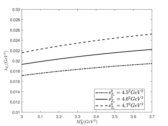
In Fig.3, we show the variation of the pole residue with the Borel parameter $M^{2}_{B}$ in the determined interval at three different values of $s^{0}_{Z_{c}}$. It is obvious that the pole residue depends weakly on $M^{2}_{B}$ and $s^{0}_{Z_{c}}$ and $\lambda_{Z_{c}}=2.1\pm 0.4\times 10^{-2}\mbox{GeV}^{5}$.

Refer to caption
Figure 3: The figure shows the dependence of the pole residue $\lambda_{Z_{c}}$ on the Borel parameter $M^{2}_{B}$ in the determined interval at three different values of $s^{0}_{Z_{c}}$.

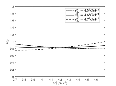
The same procedure can be done for the sum rule of the magnetic moment. The results are shown in Fig.4, from which the value of $G_{M}(0)$ can be read as $G_{M}(0)=0.82^{+0.17}_{-0.07}$. Finally, we obtain

$$\mu_{Z_{c}}=G_{M}(0)\frac{e}{2m_{Z_{c}}}=0.82^{+0.17}_{-0.07}\frac{e}{2m_{Z_{c}}}=0.19^{+0.04}_{-0.01}\mu_{N},$$ (25)

where $\mu_{N}$ is the nucleon magneton.

Refer to caption
Refer to caption
Refer to caption
Figure 4: (a) shows the various condensates as functions of $M^{2}_{B}$ with $\sqrt{s^{0}_{Z_{c}}}=4.6\mbox{GeV}$; (b) presents $RP_{1}$ and $RH_{1}$ varying with $M^{2}_{B}$ at $\sqrt{s^{0}_{Z_{c}}}=4.6\mbox{GeV}$; (c) depicts the dependence of $G_{M}$ on $M^{2}_{B}$ in the determined interval at three different values of $s^{0}_{Z_{c}}$.

In Ref.wangzhigang , the author gave $\mu_{Z_{c}}=0.47^{+0.27}_{-0.22}\mu_{N}$ assuming $Z_{c}(3900)$ as an axialvector tetraquark state by the same method used in this article. In Ref.U.Ozdem , $\mu_{Z_{c}}=0.67\pm 0.32\mu_{N}$ was predicted using light-cone sum rule under the axialvector tetraquark assumption. In Table 2, we summarize the values of the magnetic moment of $Z_{c}(3900)$ under different assumptions about the quark configuration and with different methods. It is obvious that the magnetic moment of $Z_{c}(3900)$ has different values if $Z_{c}(3900)$ has different quark configurations. The theoretical predictions can be confronted to the experimental data in the future and give important information about the inner structure of $Z_{c}(3900)$ state.

Table 2: The magnetic moment of $Z_{c}(3900)$($\mu_{N}$ is the nucleon magneton).
Quark Configuration Method Value
Axialvector Tetraquark Light-Cone Sum Rule $0.67\pm 0.32\mu_{N}$U.Ozdem
Axialvector Tetraquark QCD Sum Rule $0.47^{+0.27}_{-0.22}\mu_{N}$wangzhigang
Axialvector Molecule QCD Sum Rule $0.19^{+0.04}_{-0.01}\mu_{N}$(this work)

IV Conclusion

In this paper, we tentatively assign $Z_{c}(3900)$ to be an axialvector molecular state, calculate its magnetic moment using the QCD sum rule method in the external weak electromagnetic field. Starting with the two-point correlation function in the external electromagnetic field and expanding it in power of the electromagnetic interaction Hamiltonian, we extract the mass and pole residue of $Z_{c}(3900)$ state from the leading term in the expansion and the magnetic moment from the linear response to the external electromagnetic field. The numerical values are $m_{Z_{c}}=3.97\pm 0.12\mbox{GeV}$ in agreement with the experimental value $m^{exp}_{Z_{c}}=3899.0\pm 3.6\pm 4.9\mbox{MeV}$, $\lambda_{Z_{c}}=2.1\pm 0.4\times 10^{-2}\mbox{GeV}^{5}$ and $\mu_{Z_{c}}=0.19^{+0.04}_{-0.01}\mu_{N}$ with $\mu_{N}$ the nucleon magneton. The prediction can be confronted to the experimental data in the future and give important information about the inner structure of $Z_{c}(3900)$ state.

Acknowledgements.
This work was supported by the National Natural Science Foundation of China under Contract No.11675263.

Appendix A The quark propagators

The full quark propagators are

$\displaystyle S^{q}_{ij}(x)=$ i​​x2​π2​x4​δi​jβˆ’mq4​π2​x2​δi​jβˆ’βŸ¨q¯​q⟩12​δi​j+iβ€‹βŸ¨q¯​q⟩48​mq​​x​δi​jβˆ’x2192β€‹βŸ¨gs​q¯​σ​G​qβŸ©β€‹Ξ΄i​j𝑖π‘₯2superscriptπœ‹2superscriptπ‘₯4subscript𝛿𝑖𝑗subscriptπ‘šπ‘ž4superscriptπœ‹2superscriptπ‘₯2subscript𝛿𝑖𝑗delimited-βŸ¨βŸ©Β―π‘žπ‘ž12subscript𝛿𝑖𝑗𝑖delimited-βŸ¨βŸ©Β―π‘žπ‘ž48subscriptπ‘šπ‘žπ‘₯subscript𝛿𝑖𝑗superscriptπ‘₯2192delimited-⟨⟩subscriptπ‘”π‘ Β―π‘žπœŽπΊπ‘žsubscript𝛿𝑖𝑗\displaystyle\frac{i\not\!{x}}{2\pi^{2}x^{4}}\delta_{ij}-\frac{m_{q}}{4\pi^{2}x^{2}}\delta_{ij}-\frac{\langle\bar{q}q\rangle}{12}\delta_{ij}+i\frac{\langle\bar{q}q\rangle}{48}m_{q}\not\!{x}\delta_{ij}-\frac{x^{2}}{192}\langle g_{s}\bar{q}\sigma Gq\rangle\delta_{ij} (26)
+i​x2​​x1152​mqβ€‹βŸ¨gs​q¯​σ​G​qβŸ©β€‹Ξ΄i​jβˆ’i​gs​ti​ja​Gμ​νa32​π2​x2​(​x​σμ​ν+σμ​ν​​x)𝑖superscriptπ‘₯2π‘₯1152subscriptπ‘šπ‘ždelimited-⟨⟩subscriptπ‘”π‘ Β―π‘žπœŽπΊπ‘žsubscript𝛿𝑖𝑗𝑖subscript𝑔𝑠subscriptsuperscriptπ‘‘π‘Žπ‘–π‘—subscriptsuperscriptπΊπ‘Žπœ‡πœˆ32superscriptπœ‹2superscriptπ‘₯2π‘₯superscriptπœŽπœ‡πœˆsuperscriptπœŽπœ‡πœˆπ‘₯\displaystyle+i\frac{x^{2}\not\!{x}}{1152}m_{q}\langle g_{s}\bar{q}\sigma Gq\rangle\delta_{ij}-i\frac{g_{s}t^{a}_{ij}G^{a}_{\mu\nu}}{32\pi^{2}x^{2}}(\not\!{x}\sigma^{\mu\nu}+\sigma^{\mu\nu}\not\!{x})
$\displaystyle+i\frac{\delta_{ij}e_{q}F_{\mu\nu}}{32\pi^{2}x^{2}}(\not\!{x}\sigma^{\mu\nu}+\sigma^{\mu\nu}\not\!{x})-\frac{\delta_{ij}e_{q}\chi\langle\bar{q}q\rangle\sigma^{\mu\nu}F_{\mu\nu}}{24}$
$\displaystyle+\frac{\delta_{ij}e_{q}\langle\bar{q}q\rangle F_{\mu\nu}}{288}(\sigma^{\mu\nu}-2\sigma^{\alpha\mu}x_{\alpha}x^{\nu})$
$\displaystyle+\frac{\delta_{ij}e_{q}\langle\bar{q}q\rangle F_{\mu\nu}}{576}[(\kappa+\xi)\sigma^{\mu\nu}x^{2}-(2\kappa-\xi)\sigma^{\alpha\mu}x_{\alpha}x^{\nu}]+\cdots$

for light quarks, and

$\displaystyle S^{Q}_{ij}(x)=i\int\frac{d^{4}k}{(2\pi)^{4}}e^{-ikx}$ $\displaystyle[\frac{\not\!{k}+m_{Q}}{k^{2}-m^{2}_{Q}}\delta_{ij}-\frac{g_{s}t^{a}_{ij}G^{a}_{\mu\nu}}{4}\frac{\sigma^{\mu\nu}(\not\!{k}+m_{Q})+(\not\!{k}+m_{Q})\sigma^{\mu\nu}}{(k^{2}-m^{2}_{Q})^{2}}$ (27)
$\displaystyle+\frac{\langle g^{2}_{s}GG\rangle}{12}\delta_{ij}m_{Q}\frac{k^{2}+m_{Q}\not\!{k}}{(k^{2}-m^{2}_{Q})^{4}}$
$\displaystyle+\frac{\delta_{ij}e_{Q}F_{\mu\nu}}{4}\frac{\sigma^{\mu\nu}(\not\!{k}+m_{Q})+(\not\!{k}+m_{Q})\sigma^{\mu\nu}}{(k^{2}-m^{2}_{Q})^{2}}+\cdots]$

for heavy quarks. In these expressions $t^{a}=\frac{\lambda^{a}}{2}$ and $\lambda^{a}$ are the Gell-Mann matrix, $g_{s}$ is the strong interaction coupling constant, and $i,j$ are color indices, $e_{Q(q)}$ is the charge of the heavy (light) quark and $F_{\mu\nu}$ is the external electromagnetic field.

Appendix B The spectral densities

On the QCD side, we carry out the OPE up to dimension-10 and dimension-8 for the spectral densities $\rho^{(0)}(s)$ and $\rho^{(1)}(s)$ respectively. The explicit expressions of the spectral densities are given below.

$$\rho^{(0)}(s)=\rho^{(d=0)}_{0}+\rho^{(d=3)}_{0}(s)+\rho^{(d=4)}_{0}(s)+\rho^{(d=5)}_{0}(s)+\rho^{(d=6)}_{0}(s)+\rho^{(d=7)}_{0}(s)+\rho^{(d=8)}_{0}(s)+\rho^{(d=10)}_{0}(s),$$ (28)

with

ρ0(d=0)​(s)=34096​π6β€‹βˆ«am​i​nam​a​x𝑑aβ€‹βˆ«bm​i​n1βˆ’a𝑑b​1a3​b3​(1βˆ’aβˆ’b)​(1+a+b)​(mc2​(a+b)βˆ’a​b​s)4,subscriptsuperscriptπœŒπ‘‘00𝑠34096superscriptπœ‹6subscriptsuperscriptsubscriptπ‘Žπ‘šπ‘Žπ‘₯subscriptπ‘Žπ‘šπ‘–π‘›differential-dπ‘Žsubscriptsuperscript1π‘Žsubscriptπ‘π‘šπ‘–π‘›differential-d𝑏1superscriptπ‘Ž3superscript𝑏31π‘Žπ‘1π‘Žπ‘superscriptsubscriptsuperscriptπ‘š2π‘π‘Žπ‘π‘Žπ‘π‘ 4\rho^{(d=0)}_{0}(s)=\frac{3}{4096\pi^{6}}\int^{a_{max}}_{a_{min}}da\int^{1-a}_{b_{min}}db\frac{1}{a^{3}b^{3}}(1-a-b)(1+a+b)(m^{2}_{c}(a+b)-abs)^{4}, (29)
ρ0(d=3)​(s)=βˆ’3​mcβ€‹βŸ¨0|q¯​q|0⟩256​π4β€‹βˆ«am​i​nam​a​x𝑑aβ€‹βˆ«bm​i​n1βˆ’a𝑑b​1a2​b2​(a+b)​(1+a+b)​(mc2​(a+b)βˆ’a​b​s)2,subscriptsuperscriptπœŒπ‘‘30𝑠3subscriptπ‘šπ‘quantum-operator-product0Β―π‘žπ‘ž0256superscriptπœ‹4subscriptsuperscriptsubscriptπ‘Žπ‘šπ‘Žπ‘₯subscriptπ‘Žπ‘šπ‘–π‘›differential-dπ‘Žsubscriptsuperscript1π‘Žsubscriptπ‘π‘šπ‘–π‘›differential-d𝑏1superscriptπ‘Ž2superscript𝑏2π‘Žπ‘1π‘Žπ‘superscriptsubscriptsuperscriptπ‘š2π‘π‘Žπ‘π‘Žπ‘π‘ 2\rho^{(d=3)}_{0}(s)=-\frac{3m_{c}\langle 0|\bar{q}q|0\rangle}{256\pi^{4}}\int^{a_{max}}_{a_{min}}da\int^{1-a}_{b_{min}}db\frac{1}{a^{2}b^{2}}(a+b)(1+a+b)(m^{2}_{c}(a+b)-abs)^{2}, (30)
$\displaystyle\rho^{(d=4)}_{0}(s)=$ mc2β€‹βŸ¨0|gs2​G​G|0⟩4096​π6β€‹βˆ«am​i​nam​a​x𝑑aβ€‹βˆ«bm​i​n1βˆ’a𝑑b​1a3​b3​(a3+b3)​(1βˆ’aβˆ’b)​(1+a+b)​(mc2​(a+b)βˆ’a​b​s)subscriptsuperscriptπ‘š2𝑐quantum-operator-product0subscriptsuperscript𝑔2𝑠𝐺𝐺04096superscriptπœ‹6subscriptsuperscriptsubscriptπ‘Žπ‘šπ‘Žπ‘₯subscriptπ‘Žπ‘šπ‘–π‘›differential-dπ‘Žsubscriptsuperscript1π‘Žsubscriptπ‘π‘šπ‘–π‘›differential-d𝑏1superscriptπ‘Ž3superscript𝑏3superscriptπ‘Ž3superscript𝑏31π‘Žπ‘1π‘Žπ‘subscriptsuperscriptπ‘š2π‘π‘Žπ‘π‘Žπ‘π‘ \displaystyle\frac{m^{2}_{c}\langle 0|g^{2}_{s}GG|0\rangle}{4096\pi^{6}}\int^{a_{max}}_{a_{min}}da\int^{1-a}_{b_{min}}db\frac{1}{a^{3}b^{3}}(a^{3}+b^{3})(1-a-b)(1+a+b)(m^{2}_{c}(a+b)-abs) (31)
+⟨0|gs2​G​G|0⟩4096​π6β€‹βˆ«am​i​nam​a​x𝑑aβ€‹βˆ«bm​i​n1βˆ’a𝑑b​1a2​b2​(a+b)​(2​a+2​bβˆ’1)​(mc2​(a+b)βˆ’a​b​s)2,quantum-operator-product0subscriptsuperscript𝑔2𝑠𝐺𝐺04096superscriptπœ‹6subscriptsuperscriptsubscriptπ‘Žπ‘šπ‘Žπ‘₯subscriptπ‘Žπ‘šπ‘–π‘›differential-dπ‘Žsubscriptsuperscript1π‘Žsubscriptπ‘π‘šπ‘–π‘›differential-d𝑏1superscriptπ‘Ž2superscript𝑏2π‘Žπ‘2π‘Ž2𝑏1superscriptsubscriptsuperscriptπ‘š2π‘π‘Žπ‘π‘Žπ‘π‘ 2\displaystyle+\frac{\langle 0|g^{2}_{s}GG|0\rangle}{4096\pi^{6}}\int^{a_{max}}_{a_{min}}da\int^{1-a}_{b_{min}}db\frac{1}{a^{2}b^{2}}(a+b)(2a+2b-1)(m^{2}_{c}(a+b)-abs)^{2},
$\displaystyle\rho^{(d=5)}_{0}(s)=$ 3​mcβ€‹βŸ¨0|gs​q¯​σ⋅G​q|0⟩256​π4β€‹βˆ«am​i​nam​a​x𝑑aβ€‹βˆ«bm​i​n1βˆ’a𝑑b​1a2​b2​(a2+b2)​(a+b)​(mc2​(a+b)βˆ’a​b​s)3subscriptπ‘šπ‘quantum-operator-product0β‹…subscriptπ‘”π‘ Β―π‘žπœŽπΊπ‘ž0256superscriptπœ‹4subscriptsuperscriptsubscriptπ‘Žπ‘šπ‘Žπ‘₯subscriptπ‘Žπ‘šπ‘–π‘›differential-dπ‘Žsubscriptsuperscript1π‘Žsubscriptπ‘π‘šπ‘–π‘›differential-d𝑏1superscriptπ‘Ž2superscript𝑏2superscriptπ‘Ž2superscript𝑏2π‘Žπ‘subscriptsuperscriptπ‘š2π‘π‘Žπ‘π‘Žπ‘π‘ \displaystyle\frac{3m_{c}\langle 0|g_{s}\bar{q}\sigma\cdot Gq|0\rangle}{256\pi^{4}}\int^{a_{max}}_{a_{min}}da\int^{1-a}_{b_{min}}db\frac{1}{a^{2}b^{2}}(a^{2}+b^{2})(a+b)(m^{2}_{c}(a+b)-abs) (32)
+3​mcβ€‹βŸ¨0|gs​q¯​σ⋅G​q|0⟩512​π4β€‹βˆ«am​i​nam​a​x𝑑aβ€‹βˆ«bm​i​n1βˆ’a𝑑b​1a​b​(a+b)​(mc2​(a+b)βˆ’a​b​s)3subscriptπ‘šπ‘quantum-operator-product0β‹…subscriptπ‘”π‘ Β―π‘žπœŽπΊπ‘ž0512superscriptπœ‹4subscriptsuperscriptsubscriptπ‘Žπ‘šπ‘Žπ‘₯subscriptπ‘Žπ‘šπ‘–π‘›differential-dπ‘Žsubscriptsuperscript1π‘Žsubscriptπ‘π‘šπ‘–π‘›differential-d𝑏1π‘Žπ‘π‘Žπ‘subscriptsuperscriptπ‘š2π‘π‘Žπ‘π‘Žπ‘π‘ \displaystyle+\frac{3m_{c}\langle 0|g_{s}\bar{q}\sigma\cdot Gq|0\rangle}{512\pi^{4}}\int^{a_{max}}_{a_{min}}da\int^{1-a}_{b_{min}}db\frac{1}{ab}(a+b)(m^{2}_{c}(a+b)-abs)
βˆ’3​mcβ€‹βŸ¨0|gs​q¯​σ⋅G​q|0⟩256​π4β€‹βˆ«am​i​nam​a​x𝑑a​1a​(1βˆ’a)​(mc2βˆ’a​(1βˆ’a)​s),3subscriptπ‘šπ‘quantum-operator-product0β‹…subscriptπ‘”π‘ Β―π‘žπœŽπΊπ‘ž0256superscriptπœ‹4subscriptsuperscriptsubscriptπ‘Žπ‘šπ‘Žπ‘₯subscriptπ‘Žπ‘šπ‘–π‘›differential-dπ‘Ž1π‘Ž1π‘Žsubscriptsuperscriptπ‘š2π‘π‘Ž1π‘Žπ‘ \displaystyle-\frac{3m_{c}\langle 0|g_{s}\bar{q}\sigma\cdot Gq|0\rangle}{256\pi^{4}}\int^{a_{max}}_{a_{min}}da\frac{1}{a(1-a)}(m^{2}_{c}-a(1-a)s),
$$\rho^{(d=6)}_{0}(s)=\frac{m^{2}_{c}\langle 0|\bar{q}q0|\rangle^{2}}{16\pi^{2}}\frac{\sqrt{s(s-4m^{2}_{c})}}{s},$$ (33)
$\displaystyle\rho^{(d=7)}_{0}(s)=$ $\displaystyle-\frac{m_{c}\langle 0|\bar{q}q0|\rangle\langle 0|g^{2}_{s}GG|0\rangle}{512\pi^{4}}\int^{a_{max}}_{a_{min}}da\int^{1-a}_{b_{min}}db\frac{1}{a^{2}}b(1+a+b)$ (34)
βˆ’mcβ€‹βŸ¨0|q¯​q|0βŸ©β€‹βŸ¨0|gs2​G​G|0⟩1536​π4β€‹βˆ«am​i​nam​a​x𝑑a​(1+a+bm​i​n)​a​s+mc2mc2,subscriptπ‘šπ‘quantum-operator-product0Β―π‘žπ‘ž0quantum-operator-product0subscriptsuperscript𝑔2𝑠𝐺𝐺01536superscriptπœ‹4subscriptsuperscriptsubscriptπ‘Žπ‘šπ‘Žπ‘₯subscriptπ‘Žπ‘šπ‘–π‘›differential-dπ‘Ž1π‘Žsubscriptπ‘π‘šπ‘–π‘›π‘Žπ‘ subscriptsuperscriptπ‘š2𝑐subscriptsuperscriptπ‘š2𝑐\displaystyle-\frac{m_{c}\langle 0|\bar{q}q|0\rangle\langle 0|g^{2}_{s}GG|0\rangle}{1536\pi^{4}}\int^{a_{max}}_{a_{min}}da(1+a+b_{min})\frac{as+m^{2}_{c}}{m^{2}_{c}},
ρ0(d=8)​(s)=⟨0|q¯​q|0βŸ©β€‹βŸ¨0|gs​q¯​σ⋅G​q|0⟩32​π2​mc2s​(sβˆ’4​mc2)​(2​mc2MB2+2​mc2sβˆ’1),subscriptsuperscriptπœŒπ‘‘80𝑠quantum-operator-product0Β―π‘žπ‘ž0quantum-operator-product0β‹…subscriptπ‘”π‘ Β―π‘žπœŽπΊπ‘ž032superscriptπœ‹2subscriptsuperscriptπ‘š2𝑐𝑠𝑠4subscriptsuperscriptπ‘š2𝑐2subscriptsuperscriptπ‘š2𝑐subscriptsuperscript𝑀2𝐡2subscriptsuperscriptπ‘š2𝑐𝑠1\rho^{(d=8)}_{0}(s)=\frac{\langle 0|\bar{q}q|0\rangle\langle 0|g_{s}\bar{q}\sigma\cdot Gq|0\rangle}{32\pi^{2}}\frac{m^{2}_{c}}{\sqrt{s(s-4m^{2}_{c})}}(2\frac{m^{2}_{c}}{M^{2}_{B}}+2\frac{m^{2}_{c}}{s}-1), (35)
$\displaystyle\rho^{(d=10)}_{0}(s)=$ $\displaystyle\frac{\langle 0|\bar{q}q|0\rangle^{2}\langle 0|g^{2}_{s}GG|0\rangle}{576\pi^{2}}\frac{1}{\sqrt{s(s-4m^{2}_{c})}}(\frac{s(s-3m^{2}_{c})}{M^{4}_{B}}-3\frac{s-2m^{2}_{c}}{M^{2}_{B}})$ (36)
+⟨0|gs​q¯​σ⋅G​q|0⟩2128​π2​mc2​sMB4​s​(sβˆ’4​mc2)​(1βˆ’mc2MB2).superscriptquantum-operator-product0β‹…subscriptπ‘”π‘ Β―π‘žπœŽπΊπ‘ž02128superscriptπœ‹2subscriptsuperscriptπ‘š2𝑐𝑠subscriptsuperscript𝑀4𝐡𝑠𝑠4subscriptsuperscriptπ‘š2𝑐1subscriptsuperscriptπ‘š2𝑐subscriptsuperscript𝑀2𝐡\displaystyle+\frac{\langle 0|g_{s}\bar{q}\sigma\cdot Gq|0\rangle^{2}}{128\pi^{2}}\frac{m^{2}_{c}s}{M^{4}_{B}\sqrt{s(s-4m^{2}_{c})}}(1-\frac{m^{2}_{c}}{M^{2}_{B}}).
$$\rho^{(1)}(s)=\rho^{(d=2)}_{1}+\rho^{(d=3)}_{1}(s)+\rho^{(d=5)}_{1}(s)+\rho^{(d=6)}_{1}(s)+\rho^{(d=7)}_{1}(s)+\rho^{(d=8)}_{1}(s),$$ (37)

with

ρ1(d=2)​(s)=βˆ’31024​π6β€‹βˆ«am​i​nam​a​x𝑑aβ€‹βˆ«bm​i​n1βˆ’a𝑑b​1a2​b2​(a+b)​(mc2​(a+b)βˆ’a​b​s)3,subscriptsuperscriptπœŒπ‘‘21𝑠31024superscriptπœ‹6subscriptsuperscriptsubscriptπ‘Žπ‘šπ‘Žπ‘₯subscriptπ‘Žπ‘šπ‘–π‘›differential-dπ‘Žsubscriptsuperscript1π‘Žsubscriptπ‘π‘šπ‘–π‘›differential-d𝑏1superscriptπ‘Ž2superscript𝑏2π‘Žπ‘superscriptsubscriptsuperscriptπ‘š2π‘π‘Žπ‘π‘Žπ‘π‘ 3\rho^{(d=2)}_{1}(s)=-\frac{3}{1024\pi^{6}}\int^{a_{max}}_{a_{min}}da\int^{1-a}_{b_{min}}db\frac{1}{a^{2}b^{2}}(a+b)(m^{2}_{c}(a+b)-abs)^{3}, (38)
ρ1(d=3)​(s)=3​mcβ€‹Ο‡β€‹βŸ¨0|q¯​q|0⟩256​π4β€‹βˆ«am​i​nam​a​x𝑑aβ€‹βˆ«bm​i​n1βˆ’a𝑑b​1a​b2​(mc2​(a+b)βˆ’a​b​s)2,subscriptsuperscriptπœŒπ‘‘31𝑠3subscriptπ‘šπ‘πœ’quantum-operator-product0Β―π‘žπ‘ž0256superscriptπœ‹4subscriptsuperscriptsubscriptπ‘Žπ‘šπ‘Žπ‘₯subscriptπ‘Žπ‘šπ‘–π‘›differential-dπ‘Žsubscriptsuperscript1π‘Žsubscriptπ‘π‘šπ‘–π‘›differential-d𝑏1π‘Žsuperscript𝑏2superscriptsubscriptsuperscriptπ‘š2π‘π‘Žπ‘π‘Žπ‘π‘ 2\rho^{(d=3)}_{1}(s)=\frac{3m_{c}\chi\langle 0|\bar{q}q|0\rangle}{256\pi^{4}}\int^{a_{max}}_{a_{min}}da\int^{1-a}_{b_{min}}db\frac{1}{ab^{2}}(m^{2}_{c}(a+b)-abs)^{2}, (39)
$\displaystyle\rho^{(d=5)}_{1}(s)=$ βˆ’mcβ€‹βŸ¨0​|q¯​q​0|⟩32​π4β€‹βˆ«am​i​nam​a​x𝑑aβ€‹βˆ«bm​i​n1βˆ’a𝑑b​1b​(mc2​(a+b)βˆ’a​b​s)subscriptπ‘šπ‘delimited-⟨⟩0Β―π‘žπ‘ž032superscriptπœ‹4subscriptsuperscriptsubscriptπ‘Žπ‘šπ‘Žπ‘₯subscriptπ‘Žπ‘šπ‘–π‘›differential-dπ‘Žsubscriptsuperscript1π‘Žsubscriptπ‘π‘šπ‘–π‘›differential-d𝑏1𝑏subscriptsuperscriptπ‘š2π‘π‘Žπ‘π‘Žπ‘π‘ \displaystyle-\frac{m_{c}\langle 0|\bar{q}q0|\rangle}{32\pi^{4}}\int^{a_{max}}_{a_{min}}da\int^{1-a}_{b_{min}}db\frac{1}{b}(m^{2}_{c}(a+b)-abs) (40)
βˆ’mc​(2β€‹ΞΊβˆ’ΞΎ)β€‹βŸ¨0|q¯​q|0⟩512​π4β€‹βˆ«am​i​nam​a​x𝑑aβ€‹βˆ«bm​i​n1βˆ’a𝑑b​1b​(mc2​(a+b)βˆ’a​b​s)subscriptπ‘šπ‘2πœ…πœ‰quantum-operator-product0Β―π‘žπ‘ž0512superscriptπœ‹4subscriptsuperscriptsubscriptπ‘Žπ‘šπ‘Žπ‘₯subscriptπ‘Žπ‘šπ‘–π‘›differential-dπ‘Žsubscriptsuperscript1π‘Žsubscriptπ‘π‘šπ‘–π‘›differential-d𝑏1𝑏subscriptsuperscriptπ‘š2π‘π‘Žπ‘π‘Žπ‘π‘ \displaystyle-\frac{m_{c}(2\kappa-\xi)\langle 0|\bar{q}q|0\rangle}{512\pi^{4}}\int^{a_{max}}_{a_{min}}da\int^{1-a}_{b_{min}}db\frac{1}{b}(m^{2}_{c}(a+b)-abs)
+3​mc​(2​κ+ΞΎ)β€‹βŸ¨0|q¯​q|0⟩256​π4β€‹βˆ«am​i​nam​a​x𝑑aβ€‹βˆ«bm​i​n1βˆ’a𝑑b​1b2​(mc2​(a+b)βˆ’a​b​s)3subscriptπ‘šπ‘2πœ…πœ‰quantum-operator-product0Β―π‘žπ‘ž0256superscriptπœ‹4subscriptsuperscriptsubscriptπ‘Žπ‘šπ‘Žπ‘₯subscriptπ‘Žπ‘šπ‘–π‘›differential-dπ‘Žsubscriptsuperscript1π‘Žsubscriptπ‘π‘šπ‘–π‘›differential-d𝑏1superscript𝑏2subscriptsuperscriptπ‘š2π‘π‘Žπ‘π‘Žπ‘π‘ \displaystyle+\frac{3m_{c}(2\kappa+\xi)\langle 0|\bar{q}q|0\rangle}{256\pi^{4}}\int^{a_{max}}_{a_{min}}da\int^{1-a}_{b_{min}}db\frac{1}{b^{2}}(m^{2}_{c}(a+b)-abs)
+mcβ€‹βŸ¨0|q¯​q|0⟩64​π4β€‹βˆ«am​i​nam​a​x𝑑a​1a​(mc2βˆ’a​(1βˆ’a)​s)subscriptπ‘šπ‘quantum-operator-product0Β―π‘žπ‘ž064superscriptπœ‹4subscriptsuperscriptsubscriptπ‘Žπ‘šπ‘Žπ‘₯subscriptπ‘Žπ‘šπ‘–π‘›differential-dπ‘Ž1π‘Žsubscriptsuperscriptπ‘š2π‘π‘Ž1π‘Žπ‘ \displaystyle+\frac{m_{c}\langle 0|\bar{q}q|0\rangle}{64\pi^{4}}\int^{a_{max}}_{a_{min}}da\frac{1}{a}(m^{2}_{c}-a(1-a)s)
βˆ’mc​(ΞΊ+ΞΎ)β€‹βŸ¨0|q¯​q|0⟩256​π4β€‹βˆ«am​i​nam​a​x𝑑a​1a​(mc2βˆ’a​(1βˆ’a)​s)subscriptπ‘šπ‘πœ…πœ‰quantum-operator-product0Β―π‘žπ‘ž0256superscriptπœ‹4subscriptsuperscriptsubscriptπ‘Žπ‘šπ‘Žπ‘₯subscriptπ‘Žπ‘šπ‘–π‘›differential-dπ‘Ž1π‘Žsubscriptsuperscriptπ‘š2π‘π‘Ž1π‘Žπ‘ \displaystyle-\frac{m_{c}(\kappa+\xi)\langle 0|\bar{q}q|0\rangle}{256\pi^{4}}\int^{a_{max}}_{a_{min}}da\frac{1}{a}(m^{2}_{c}-a(1-a)s)
$\displaystyle\rho^{(d=6)}_{1}(s)=$ $\displaystyle-\frac{m^{2}_{c}\langle 0|g^{2}_{s}GG|0\rangle}{2048\pi^{6}}\int^{a_{max}}_{a_{min}}da\int^{1-a}_{b_{min}}db\frac{1}{b^{2}}a(a+b)$ (41)
+3β€‹βŸ¨0|gs2​G​G|0⟩4096​π6β€‹βˆ«am​i​nam​a​x𝑑aβ€‹βˆ«bm​i​n1βˆ’a𝑑b​1b​(mc2​(a+b)βˆ’a​b​s)3quantum-operator-product0subscriptsuperscript𝑔2𝑠𝐺𝐺04096superscriptπœ‹6subscriptsuperscriptsubscriptπ‘Žπ‘šπ‘Žπ‘₯subscriptπ‘Žπ‘šπ‘–π‘›differential-dπ‘Žsubscriptsuperscript1π‘Žsubscriptπ‘π‘šπ‘–π‘›differential-d𝑏1𝑏subscriptsuperscriptπ‘š2π‘π‘Žπ‘π‘Žπ‘π‘ \displaystyle+\frac{3\langle 0|g^{2}_{s}GG|0\rangle}{4096\pi^{6}}\int^{a_{max}}_{a_{min}}da\int^{1-a}_{b_{min}}db\frac{1}{b}(m^{2}_{c}(a+b)-abs)
βˆ’3β€‹βŸ¨0|gs2​G​G|0⟩4096​π6β€‹βˆ«am​i​nam​a​x𝑑a​1a​(mc2βˆ’a​(1βˆ’a)​s)3quantum-operator-product0subscriptsuperscript𝑔2𝑠𝐺𝐺04096superscriptπœ‹6subscriptsuperscriptsubscriptπ‘Žπ‘šπ‘Žπ‘₯subscriptπ‘Žπ‘šπ‘–π‘›differential-dπ‘Ž1π‘Žsubscriptsuperscriptπ‘š2π‘π‘Ž1π‘Žπ‘ \displaystyle-\frac{3\langle 0|g^{2}_{s}GG|0\rangle}{4096\pi^{6}}\int^{a_{max}}_{a_{min}}da\frac{1}{a}(m^{2}_{c}-a(1-a)s)
$\displaystyle-\frac{m^{2}_{c}\chi\langle 0|\bar{q}q|0\rangle^{2}}{32\pi^{2}}\frac{\sqrt{s(s-4m^{2}_{c})}}{s},$
$\displaystyle\rho^{(d=7)}_{1}(s)=$ $\displaystyle\frac{m_{c}\chi\langle 0|\bar{q}q|0\rangle\langle 0|g^{2}_{s}GG|0\rangle}{1024\pi^{4}}\int^{a_{max}}_{a_{min}}da\int^{1-a}_{b_{min}}db\frac{a}{b^{2}}$ (42)
+Ο‡β€‹βŸ¨0|q¯​q|0βŸ©β€‹βŸ¨0|gs2​G​G|0⟩3072​π4β€‹βˆ«am​i​nam​a​x𝑑a​a​s+3​mc2mcπœ’quantum-operator-product0Β―π‘žπ‘ž0quantum-operator-product0subscriptsuperscript𝑔2𝑠𝐺𝐺03072superscriptπœ‹4subscriptsuperscriptsubscriptπ‘Žπ‘šπ‘Žπ‘₯subscriptπ‘Žπ‘šπ‘–π‘›differential-dπ‘Žπ‘Žπ‘ 3subscriptsuperscriptπ‘š2𝑐subscriptπ‘šπ‘\displaystyle+\frac{\chi\langle 0|\bar{q}q|0\rangle\langle 0|g^{2}_{s}GG|0\rangle}{3072\pi^{4}}\int^{a_{max}}_{a_{min}}da\frac{as+3m^{2}_{c}}{m_{c}}
+3​mcβ€‹βŸ¨0​|gs​q¯​σ⋅G​q​0|⟩256​π4β€‹βˆ«am​i​nam​a​x𝑑aβ€‹βˆ«bm​i​n1βˆ’a𝑑b​ab3subscriptπ‘šπ‘delimited-⟨⟩0β‹…subscriptπ‘”π‘ Β―π‘žπœŽπΊπ‘ž0256superscriptπœ‹4subscriptsuperscriptsubscriptπ‘Žπ‘šπ‘Žπ‘₯subscriptπ‘Žπ‘šπ‘–π‘›differential-dπ‘Žsubscriptsuperscript1π‘Žsubscriptπ‘π‘šπ‘–π‘›differential-dπ‘π‘Žπ‘\displaystyle+\frac{3m_{c}\langle 0|g_{s}\bar{q}\sigma\cdot Gq0|\rangle}{256\pi^{4}}\int^{a_{max}}_{a_{min}}da\int^{1-a}_{b_{min}}db\frac{a}{b}
βˆ’3​mcβ€‹βŸ¨0​|gs​q¯​σ⋅G​q​0|⟩256​π4β€‹βˆ«am​i​nam​a​x𝑑a​1βˆ’aa3subscriptπ‘šπ‘delimited-⟨⟩0β‹…subscriptπ‘”π‘ Β―π‘žπœŽπΊπ‘ž0256superscriptπœ‹4subscriptsuperscriptsubscriptπ‘Žπ‘šπ‘Žπ‘₯subscriptπ‘Žπ‘šπ‘–π‘›differential-dπ‘Ž1π‘Žπ‘Ž\displaystyle-\frac{3m_{c}\langle 0|g_{s}\bar{q}\sigma\cdot Gq0|\rangle}{256\pi^{4}}\int^{a_{max}}_{a_{min}}da\frac{1-a}{a}
βˆ’3​mc3β€‹βŸ¨0​|gs​q¯​σ⋅G​q​0|⟩512​π4​1s​(sβˆ’4​mc2)3subscriptsuperscriptπ‘š3𝑐delimited-⟨⟩0β‹…subscriptπ‘”π‘ Β―π‘žπœŽπΊπ‘ž0512superscriptπœ‹41𝑠𝑠4subscriptsuperscriptπ‘š2𝑐\displaystyle-\frac{3m^{3}_{c}\langle 0|g_{s}\bar{q}\sigma\cdot Gq0|\rangle}{512\pi^{4}}\frac{1}{\sqrt{s(s-4m^{2}_{c})}}
+3​mcβ€‹βŸ¨0​|gs​q¯​σ⋅G​q​0|⟩1024​π4​s​(sβˆ’4​mc2)s,3subscriptπ‘šπ‘delimited-⟨⟩0β‹…subscriptπ‘”π‘ Β―π‘žπœŽπΊπ‘ž01024superscriptπœ‹4𝑠𝑠4subscriptsuperscriptπ‘š2𝑐𝑠\displaystyle+\frac{3m_{c}\langle 0|g_{s}\bar{q}\sigma\cdot Gq0|\rangle}{1024\pi^{4}}\frac{\sqrt{s(s-4m^{2}_{c})}}{s},
$\displaystyle\rho^{(d=8)}_{1}(s)=$ βˆ’mc2β€‹Ο‡β€‹βŸ¨0​|q¯​q​|0βŸ©β€‹βŸ¨0|​gs​q¯​σ⋅G​q​0|⟩64​π2​1s​(sβˆ’4​mc2)​(mc2MB2+mc2sβˆ’1)subscriptsuperscriptπ‘š2π‘πœ’delimited-⟨⟩0β‹…Β―π‘žπ‘žket0bra0subscriptπ‘”π‘ Β―π‘žπœŽπΊπ‘ž064superscriptπœ‹21𝑠𝑠4subscriptsuperscriptπ‘š2𝑐subscriptsuperscriptπ‘š2𝑐subscriptsuperscript𝑀2𝐡subscriptsuperscriptπ‘š2𝑐𝑠1\displaystyle-\frac{m^{2}_{c}\chi\langle 0|\bar{q}q|0\rangle\langle 0|g_{s}\bar{q}\sigma\cdot Gq0|\rangle}{64\pi^{2}}\frac{1}{\sqrt{s(s-4m^{2}_{c})}}(\frac{m^{2}_{c}}{M^{2}_{B}}+\frac{m^{2}_{c}}{s}-1) (43)
$\displaystyle+\frac{m^{4}_{c}\langle 0|\bar{q}q|0\rangle^{2}}{48\pi^{2}}\frac{1}{\sqrt{s(s-4m^{2}_{c})}}(\frac{1}{M^{2}_{B}}+\frac{2}{s})$
$\displaystyle+\frac{m^{4}_{c}(2\kappa-\xi)\langle 0|\bar{q}q|0\rangle^{2}}{192\pi^{2}}\frac{1}{s\sqrt{s(s-4m^{2}_{c})}}$
$\displaystyle+\frac{m^{4}_{c}(\kappa+\xi)\langle 0|\bar{q}q|0\rangle^{2}}{96\pi^{2}}\frac{1}{\sqrt{s(s-4m^{2}_{c})}}(\frac{1}{M^{2}_{B}}+\frac{1}{s})$
$\displaystyle-\frac{m^{2}_{c}(2\kappa+\xi)\langle 0|\bar{q}q|0\rangle^{2}}{64\pi^{2}}\frac{1}{\sqrt{s(s-4m^{2}_{c})}}.$

In the above equations, $a_{max}=\frac{1+\sqrt{1-\frac{4m^{2}_{c}}{s}}}{2}$, $a_{min}=\frac{1-\sqrt{1-\frac{4m^{2}_{c}}{s}}}{2}$ and bm​i​n=a​mc2a​sβˆ’mc2subscriptπ‘π‘šπ‘–π‘›π‘Žsubscriptsuperscriptπ‘š2π‘π‘Žπ‘ subscriptsuperscriptπ‘š2𝑐b_{min}=\frac{am^{2}_{c}}{as-m^{2}_{c}}.

References

  • (1) M. Ablikim et al, Phys. Rev. Lett. 110 (2013) 252001.
  • (2) Z. Q. Liu et al, Phys. Rev. Lett. 110 (2013) 252002.
  • (3) T. Xiao, S. Dobbs, A. Tomaradze and K. K. Seth, Phys. Lett. B727 (2013) 366.
  • (4) M. Ablikim et al, Phys. Rev. Lett. 119 (2017) 072001.
  • (5) Y. R. Liu, H. X. Chen, W. Chen, X. Liu, and S. L. Zhu, Prog. Part. Nucl. Phys. 107 (2019) 237; H. X. Chen, W. Chen, X. Liu, Y. R. Liu and S. L. Zhu, Rept. Prog. Phys. 80 (2017) no. 7, 076201; H. X. Chen, W. Chen, X. Liu and S. L. Zhu, Phys. Rept. 639 (2016) 1.
  • (6) M. A. Shifman, A. I. Vainshtein and V. I. Zakharov, Nucl. Phys. B147 (1979) 385; Nucl. Phys. B147 (1979) 448.
  • (7) I. I. Balitsky and A. V. Yung, Phys. Lett. B129 (1983) 328.
  • (8) B. L. Ioffe and A. V. Smilga, Nucl. Phys. B232 (1984) 109.
  • (9) B. L. Ioffe and A. V. Smilga, Phys. Lett. B133 (1983) 436.
  • (10) C. B. Chiu, J. Pasupathy and S. L. Wilson, Phys. Rev. D33 (1986) 1961.
  • (11) J. Pasupathy, J. P. Singh, S. L. Wilson and C. B. Chiu, Phys. Rev. D36 (1986) 1442.
  • (12) S. L. Wilson, J. Pasupathy and C. B. Chiu, Phys. Rev. D36 (1987) 1451.
  • (13) S. Zhu, W. Hwang and Z. Yang, Phys. Rev. D57 (1998) 1527.
  • (14) F. X. Lee, Phys. Rev. D57 (1998) 1801.
  • (15) F. X. Lee, Phys. Lett. B419 (1998) 14.
  • (16) J. Dey, M. Dey and A. Iqubal, Phys. Lett. B477 (2000) 125.
  • (17) M. Sinha, A. Iqubal, M. Dey and J. Dey, Phys. Lett. B610 (2005) 283.
  • (18) A. Samsonov, Phys. Atom. Nucl. 68 (2005) 114.
  • (19) Z. G. Wang, Eur. Phys. J. C78 (2018)4 297.
  • (20) C. Y. Cui, X. H. Liao, Y. L. Liu and M. Q. Huang, J. Phys. G41 (2014) 075003.
  • (21) M. Tanabashi et al[Particle Data Group], Phys. Rev. D98 (2018) 030001.
  • (22) P. Ball, V. M. Braun and N. Kivel, Nucl. Phys. B649 (2003) 263.
  • (23) U. Ozdem and K. Azizi, Phys. Rev. D96 (2017) 074030.