Communication-Efficient Federated Learning via Optimal Client Sampling

Abstract

Federated learning (FL) ameliorates privacy concerns in settings where a central server coordinates learning from data distributed across many clients. The clients train locally and communicate the models they learn to the server; aggregation of local models requires frequent communication of large amounts of information between the clients and the central server. We propose a novel, simple and efficient way of updating the central model in communication-constrained settings based on collecting models from clients with informative updates and estimating local updates that were not communicated. In particular, modeling the progression of model’s weights by an Ornstein-Uhlenbeck process allows us to derive an optimal sampling strategy for selecting a subset of clients with significant weight updates. The central server collects updated local models from only the selected clients and combines them with estimated model updates of the clients that were not selected for communication. We test this policy on a synthetic dataset for logistic regression and two FL benchmarks, namely, a classification task on EMNIST and a realistic language modeling task using the Shakespeare dataset. The results demonstrate that the proposed framework provides significant reduction in communication while maintaining competitive or achieving superior performance compared to a baseline. Our method represents a new line of strategies for communication-efficient FL that is orthogonal to the existing user-local methods such as quantization or sparsification, thus complementing rather than aiming to replace those existing methods.

1 Introduction

Federated learning (FL) is a privacy-preserving framework for training machine learning models in settings where the data is distributed across many clients. Such settings are common in applications that involve mobile devices (McMahan et al., 2017), automated vehicles, and Internet-of-Things (IoT) systems, as well as in cross-silo applications including healthcare (Ribero et al., 2020) and banking. In FedAvg, the baseline FL procedure proposed in (McMahan et al., 2017) (included in the supplementary material as Algorithm 4), a server distributes an initial model to clients who independently update the model using their local training data. These updates are aggregated by the server which broadcasts a new global model to the clients and selects a subset of them to start a new round of local training; the procedure is repeated until convergence. Since clients communicate only their models to the server, FL offers data security that can be further strengthened using privacy mechanisms including those that provide differential privacy guarantees (Abadi et al., 2016; Wu et al., 2017; McMahan et al., 2018).

The number of clients in FL systems may be in the order of millions, and the models that they locally train could be rather large; for example, VGG-16, the widely known neural network for image recognition has 138M parameters (Simonyan and Zisserman, 2014), weighing 526MB when represented by 32 bits. Moreover, many settings where FL is applied are highly dynamic (e.g., mobile devices, IoT), with new users joining at any moment and old users continuing to generate new data. Such settings may lead to a large number of training rounds and clients’ model uploads, even though the contributions of some locally updated models to the global one may be rather limited. Since transmitting large models requires considerable communication resources, it is desirable to reduce the amount of information that has to be collected by the server. This is being explored in a promising line of work focused on reducing each client’s communication budget by compressing the ML model through strategies such as quantization and sparsification (Tang et al., 2019; Konečnỳ et al., 2016; Suresh et al., 2017; Konečnỳ and Richtárik, 2018; Alistarh et al., 2017; Horvath et al., 2019).

In the existing FL systems, the number of clients participating in each round of updates (and, therefore, the required communication budget) is typically fixed. Yet the contributions of many clients in any given round may have limited impact, especially near convergence. Following this intuition, we propose a novel approach to reducing communication in FL by identifying and transmitting only the client updates that are deemed informative. In particular, we model the progression of users’ vector of weights during stochastic gradient descent (SGD) as a multidimensional stochastic process, and let each user decide whether or not to send an update to the server based on how informative is the observed segment of a sample path (e.g., how far is the process from its steady-state). Specifically, we rely on the Ornstein-Uhlenbeck process (OU) – a continuous stochastic process parameterized by the mean and covariance functions – and interpret weights in SGD iterations as the points obtained by discretizing a sample path of the underlying OU process. Relying on this connection, we borrow techniques for optimal sampling of OU processes and adapt them to the problem of optimal client sampling. The optimal strategy turns out to be a simple threshold on the update’s norm and can thus be efficiently implemented at the client side.

We develop a dynamic strategy for selecting the threshold value; the threshold varies adaptively during the training process. In particular, after a round of training on local data, the clients share their updates’ norm with the server; the server computes a threshold and broadcasts it to the clients who in turn rely on the received threshold to decide whether or not to send their updates to the server. Updates of the clients who chose not to communicate are predicted using the server’s estimate of the parameters of the underlying OU process. Heuristics that discard small model updates in distributed learning have previously been proposed Hsieh et al. (2017); Chen et al. (2018); Singh et al. (2019); however, in this prior work the missing models are replaced with either historic values or simply ignored. In contrast, we rely on our OU model assumptions to estimate missing model updates, and demonstrate that such a non-trivial update boosts performance of the FL scheme.

Efficacy of the proposed formulation is demonstrated in practical settings where we show that it may reduce communication during an FL training loop up to 50 % while achieving the same rate of convergence and competitive (or better) model accuracy. In particular, we test our methods on a logistic regression with synthetic data, and two FL benchmark tests: a 62 character classification task on a real federated dataset EMNIST Cohen et al. (2017) using a convolutional neural network architecture, and on the Shakespeare dataset McMahan et al. (2017) where we trained a model for a character prediction task.

We summarize our proposed scheme in Fig 1. Our approach requires two major modifications of the original Federated Averaging algorithm (FedAvg, included for completeness in Sec A.1 as Algorithm 4). As in the original FedAvg McMahan et al. (2017), the server selects $N$ clients and broadcasts the current model, but now includes a threshold $\tau_{t}$ (Fig 1(a)). The selected clients train for $E$ epochs and evaluate how much their update differs from the original model by computing the norm of the difference between the models. If this difference exceeds threshold $\tau_{t}$, the update is transmitted; otherwise, only the norm of the update is sent to the server (Fig 1(b)). The server relies on the model history to estimate parameters of the underlying OU process, and uses them to predict missing clients updates (rather than zeroing or ignoring these clients updates). This is described in details in Sec 3. By combining received and estimated updates, the server generates a new model. Finally, the server uses the collected local model norms to produce a new threshold for the next round; the described procedure repeats until a stopping criterion is met.

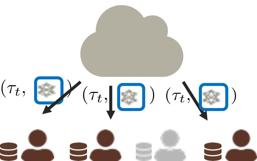
(a) Server selects $N$ clients, and broadcasts the current global model and threshold.

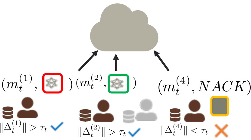
(b) Client $k$ locally updates her model and computes $\Delta_{t}^{(k)}$. If clients meet the threshold, they send back the update and its norm (in the illustration, clients 1 and 2). Otherwise, clients only send the norm of their update (client 4).

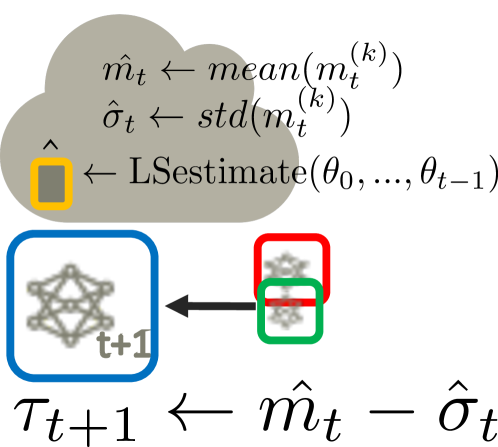
(c) In round $t$, server: (i) computes the mean and standard deviation of the received norms of the updates; (ii) estimates missing clients updates via (7); (iii) updates the global model and computes the threshold for round $t+1$.

Figure 1: One round $(t)$ of communication efficient federated learning system through client sampling and estimation

2 Background and Related Work

2.1 Federated Learning

The FL algorithm introduced in McMahan et al. (2017), FedAvg, requires a random subset of clients to send their updates to the server after having trained locally for $E$ epochs on mini-batches of size $B$. For more details, please see Algorithm 4 in the supplementary document. In subsequent years, various aspects of FL systems have attracted a lot of attention including privacy and security Abadi et al. (2016); Geyer et al. (2017); Amin et al. (2019); Bonawitz et al. (2016), optimization Reddi et al. (2020), adversarial attacks Bagdasaryan et al. (2018); Bhagoji et al. (2018) and personalization Smith et al. (2017) – see Kairouz et al. (2019) for a comprehensive overview. Our focus is on communication challenges in FL.

2.2 Communication reduction strategies

Highly relevant to our problem is the line of research on distributed estimation under communication constraints (see, e.g., Boyd et al. (2011); Duchi et al. (2011); Balcan et al. (2012); Zhang et al. (2013b) and the references therein). Recently, work by Zhang et al. (2013a); Braverman et al. (2016); Han et al. (2018); Acharya et al. (2018) provided bounds on the minimax risk, i.e., the worst-case estimation error for a distributed system operating under a constraint on the maximum number of bits that remote nodes are allowed to transmit. Under the same constraint, Barnes et al. (2019) leveraged Fisher information to derive lower bounds on the estimation error.

Existing schemes for reducing communication overhead in FL systems typically perform compression on the client side and thus require additional computation for encoding and decoding. Deterministic approaches such as low rank approximation, sparsification, subsampling, and quantization (Konečnỳ et al., 2016; Alistarh et al., 2017; Horvath et al., 2019), as well as randomized approaches including random rotations and stochastic rounding (Suresh et al., 2017) and randomized approximation (Konečnỳ and Richtárik, 2018), can be used to reduce the communication while maintaining high accuracy. Note that these methods may be leveraged on the server side as well (Caldas et al., 2018).

Orthogonal to compression-based methods, approaches that dismiss updates of some workers have been proposed in the distributed learning literature Hsieh et al. (2017); Chen et al. (2018); Singh et al. (2019). Hsieh et al. (2017) propose to threshold significant updates where the significance is measured in terms of relative magnitude change; only those updates that exceed a threshold are communicated and averaged. A major drawback of this method is ignoring updates near convergence, thus causing stagnation in training. Our experiments demonstrate that such effects lead to unstable behavior, particularly in the case of heterogeneous data. Thresholding method in Chen et al. (2018) explores settings that rely on a central server for coordination and proposes to replace the update of a client that did not communicate by the client’s previous update. This approach requires the server to store for all clients their updates from the previous round. Singh et al. (2019) considers a similar approach for the fully decentralized setting, with a notable difference of setting the threshold according to a schedule $c_{t}=o(t)$ to guarantee convergence. These last two approaches are challenging to implement in FL settings because the number of clients in FL can be on the order of millions, and it is thus very likely that in each training round new clients are sampled. Therefore, updates of the clients that did not communicate should be replaced by the latest model they received, likely slowing down the training process. Nevertheless, this direction is worth pursuing since reducing the number of clients that send updates to a server may significantly reduce the amount of communication, as demonstrated by the heuristics which impose limits on the uploading times of updates (Nishio and Yonetani, 2019). On a different vein, Cho et al. (2020) theoretically analyzes the effect of biased sampling on convergence.

Another approach to learning under resource constraints is focused on reducing the overall model complexity, e.g., by bounding the model size (Lin et al., 2016; Oktay et al., 2019), pruning (Han et al., 2015; Aghasi et al., 2016; Dong et al., 2017; Zhu and Gupta, 2017), or restricting weights to be binary (Courbariaux et al., 2015). Adaptation of these methods to FL and their analysis in such context are open research questions.

2.3 Ornstein-Uhlenbeck Process

In this section we provide a brief background on the Ornstein-Uhlenbeck process and overview an efficient procedure for the estimation of the process parameters. These concepts are at the core of our proposed approach to estimating client updates that due to thresholding are not communicated to the server in FL systems.

Definition.

The Ornstein-Uhlenbeck process (OU) is a stationary Gauss-Markov process which, over time, drifts towards its mean function. Unlike the Wiener process whose drift is constant, the drift of the OU process depends on how far is its current realization from the mean. The OU processes have been extensively studied in a wide range of fields including physics (Lemons and Langevin, 2002), finance (Stein and Stein, 1991; Evans et al., 1994; Siu-tang and Xin, 2015), and biology (Ricciardi and Sacerdote, 1979; Rohlfs et al., 2014), to name a few. Formally, the OU process $\{x_{t}\}_{t}$ is described by the stochastic differential equation

$$d\theta_{t}=\lambda(\mu-\theta_{t})dt+\sigma dW_{t},$$ (1)

where $W_{t}$ denotes the standard Wiener process. Expression (1) specifies the process that is drifting towards $\mu$ with velocity $\lambda$, and has volatility driven by a Brownian motion with variance $\sigma$.

Estimating parameters of the OU process.

Various techniques for estimating parameters of the OU process from the observations of its sample path have been proposed in literature, including least-squares, maximum likelihood (Liptser and Shiryaev, 2013) and Jackknife method (Shao and Tu, 2012). For convenience, we here summarize the computationally efficient least-squares solution. First, note that by discretizing the continuous OU process we obtain

$$\theta_{t+1}=e^{-\lambda\Delta t}\theta_{t}+(1-e^{-\lambda\Delta t})\mu+\sigma\sqrt{\frac{1-e^{-\lambda\Delta t}}{2\lambda}}\Delta W_{t},$$ (2)

where $\Delta t$ denotes the discretization (sampling) period and $\Delta W_{t}$ are i.i.d. increments of the Wiener process. This leads to a linear measurement model

$$\theta_{t+1}=a\theta_{t}+b+\epsilon_{t}$$ (3)

where $\epsilon_{t}$ denotes i.i.d. noise and where

$$a=e^{-\lambda\Delta t},\;b=\mu(1-e^{\lambda\Delta t}),\;std(\epsilon_{t})=\sigma\sqrt{\frac{(1-e^{2\lambda\Delta})}{2\lambda}}.$$

To enable efficient online (i.e., recursive) estimation of the relevant process parameters, let us define

$$S_{x,t}=\sum_{i=1}^{t}\theta_{i-1}, S_{y,t}=\sum_{i=1}^{t}\theta_{i},$$

$$S_{xx,t}=\sum_{i=1}^{t}\theta^{2}_{i-1}, S_{yy,t}=\sum_{i=1}^{t}\theta_{i}^{2},$$

$$S_{xy,t}=\sum_{i=1}^{t}\theta_{i-1}\theta_{i},$$ (4)

where $\theta_{1},\theta_{2},\dots\theta_{t}$ denote samples of the OU process. It is straightforward to show that the least-square estimates of $a_{t}$, $b_{t}$ and $std(\epsilon_{t})$ given $\theta_{1},\theta_{2},\dots\theta_{t}$ can be found as

$$\hat{a}_{t}=\frac{tS_{xy,t}-S_{x,t}S_{y,t}}{tS_{xx,t}S_{xx,t}}, \quad\hat{b}_{t}=\frac{S_{y,t}-\hat{a}_{t}S_{x,t}}{t}$$ (5)

and

$$\widehat{std(\epsilon_{t})}=\sqrt{\frac{tS_{yy,t}-S_{y,t}^{2}-\hat{a}_{t}(tS_{xy,t}-S_{x,t}S_{y,t})}{t(t-1)}}.$$

Finally, the next value of the sample path, $\theta_{t+1}$, is predicted as

$$\hat{\theta}_{t+1}=\hat{a}_{t}\theta_{t}+\hat{b}_{t}.$$ (6)

Optimal sampling of the OU process.

Rate-constrained sampling of stochastic processes has been widely studied in literature, primarily in the context of communications and control (Imer and Basar, 2005; Bommannavar and Başar, 2008; Nayyar et al., 2013; Rabi et al., 2012; Nar and Başar, 2014; Sun et al., 2017; Ornee and Sun, 2019; Guo and Kostina, 2020). In (Imer and Basar, 2005; Bommannavar and Başar, 2008), this problem is studied for random i.i.d. sequences and Gauss-Markov processes; Nayyar et al. (2013) present a similar study in the scenario where the nodes of a sensor network collaboratively estimate environment while operating under energy constraints that limit the amount of information sensors can transmit to a central processor. Rabi et al. (2012) study linear diffusion processes and formulate sampling as a stopping time problem; Nar and Başar (2014) extend these results to multidimensional problems.

The setting where samples are observed locally (by nodes/clients) but used for estimation only if communicated to the central processor is studied in (Sun et al., 2017; Ornee and Sun, 2019). As shown there, thresholding the signal magnitude increment is an optimal sampling policy for estimating parameters of an OU process. An extension of these results to a larger class of continuous Markov processes with regularity conditions is considered in Guo and Kostina (2020).

Connection between OU processes and SGD.

Recently, Blanc et al. (2019); Wang (2017); Li et al. (2018); Mandt et al. (2016) have studied SGD in various settings by relying on stochastic differential equation models. Mandt et al. (2016) model SGD as an OU process and leverage its properties to derive optimal model parameters. Wang (2017) investigates asymptotic behaviour of descent algorithms using stochastic process models. Li et al. (2018) show that SGD can be used for statistical inference and demonstrate that the average of SGD sequences can be approximated by an OU process. Blanc et al. (2019) show that when learning a neural network with SGD and independent label noise, the dynamics of weight updates can be interpreted as an OU process. This connection is formalized in the next section.

3 Efficient Training via Client Sampling

Here we introduce the techniques from optimal process sampling to FL systems, with the goal of reducing communication and improving accuracy. In particular, we present a strategy where a client transmits its weights to the server only if the norm of the client’s model update exceeds a pre-determined threshold, and provide a non-trivial estimator of the model updates that did not meet the communication threshold.

For convenience, the notation, including definition of variables, is summarized in Table 1

Variable	Definition
$N$	Number of clients to sample
	each round
$T$	Total number of rounds
$\tau_{t}$	Threshold sent by the server to
	users at the beginning of round $t$
$\theta_{t}$	Global model at round $t$
$\theta^{(k)}_{t+1}$	Local model at the end of
	round $t$ at client $k$
$\Delta^{(k)}_{t}:=\theta^{(k)}_{t+1}-\theta_{t}$	Update for client $k$ at round $t$
$m_{t}^{(k)}:=\|\Delta^{(k)}_{t}\|_{2}$	$\ell_{2}$- norm of client $k$ update at $t$
$m_{t}$	Mean of updates norms at the
	end of round $t$
$s_{t}$	Standard deviation of norms
	at the end of round $t$

Table 1: Notation used in the paper.

3.1 SGD as an OU process

Consider the loss function $\mathcal{L}(\theta;X)=\sum_{i=1}^{N}\ell_{i}(\theta)$, where $X$ is a dataset with $N$ samples and $\ell_{i}(\theta)$ is the loss of point $x_{i}\in X$ for $i=1,\dots,N$. In gradient descent, $\mathcal{L}$ is minimized by evaluating in each iteration an approximation of the gradient using a mini-batch $\mathcal{S}\subseteq X$ of the data. In particular,

$$\theta_{t+1}\leftarrow\theta_{t}-\frac{\eta}{|\mathcal{S}|}\sum_{i\in\mathcal{S}}g_{i}(\theta).$$

The following observations and assumptions are commonly encountered in literature (see, e.g., (Mandt et al., 2016)).

Observation 1: The central limit theorem implies that $\frac{1}{|\mathcal{S}|}\sum_{i\in\mathcal{S}}g_{i}(\theta)\rightarrow\mathcal{N}(g(\theta),B(\theta)B(\theta)^{T})$, where $g(\theta)$ denotes the full gradient and $B(\theta)B(\theta)^{T}$ is the corresponding covariance matrix.

Assumption 1: When $\theta$ approaches a stationary value, $B(\theta)=B$ is constant (Mandt et al., 2016).

Assumption 2: The iterates $\theta_{t}$ lie in a region where the loss can be approximated by a quadratic form $\mathcal{L}(\theta)=\frac{1}{2}\theta^{T}A\theta$ (readily justified in the case of smooth loss functions), and the process reaches a quasi-stationary distribution around a local minimum.

Predicated on the above, the discrete process

$$\Delta\theta=\theta_{t+1}-\theta_{t}\approx-\eta g(\theta)-\sqrt{\frac{\eta}{N}}B\mathcal{N}(0,\eta I)$$

can be interpreted as obtained by discretizing the OU process

$$d\theta_{t}=-g(\theta)dt+\sqrt{\frac{\eta}{N}}BdW_{t}=-A\theta_{t}dt+\sqrt{\frac{\eta}{N}}BdW_{t}$$

in the relative proximity of the steady state. In the supplementary material (Sec B.1) we illustrate these arguments by showing plots of the sample paths of randomly selected weights in a convolutional neural network trained on the Fashion MNIST dataset Xiao et al. (2017) using SGD with a constant learning rate. At each iteration, distribution of the weight increments is approximately Gaussian; as expected, the weights follow trajectories typical of OU sample paths.

3.2 Optimal sampling of OU processes in FL settings

The OU process sampling strategies discussed in Sec 2 assume a network of nodes with unlimited access to the process, while the estimator is located on a central server. When a sampling frequency constraint (i.e., uplink bandwidth) limits the number of samples that could be collected by the server, the nodes should locally decide when to send an update. Guo et al. Guo and Kostina (2020) show that the optimal strategy minimizing Mean Squared Error (MSE) is to sample at time $\tau=\inf\{t\geq 0:|\theta_{t}-\mathbb{E}[\theta_{t}|\theta_{0}]|>\gamma\}$, and that the optimal decoding policy is given by $\hat{\theta}_{t}=\mathbb{E}[\theta_{t}|\theta_{0}]$, for $t\in[0,\tau)$. In particular, for the OU process in (1),

$$\hat{\theta}_{t}=e^{-\lambda\Delta t}\theta_{0}+(1-e^{-\lambda\Delta t})\mu.$$ (7)

To establish a connection to FL, we recall the arguments from the previous subsection and note that in each round $t$ of an FL procedure, client $k$ “observes” a partial sample path of an OU process that terminates in $\theta_{t}^{(k)}$ (i.e., the client records progression of its weights during local training); the sample path starts from point $\theta_{t}$ (i.e., model weights) broadcasted by the server at the beginning of the current training round. Let $\Delta^{(k)}_{t}:=\theta^{(k)}_{t}-\theta_{t}$ be the difference between a locally updated (by client $k$) and the previously broadcasted model. Invoking the above sampling optimality results, we propose to schedule transmission of updates if $\|\Delta^{(k)}_{t}\|_{2}$ exceeds a judiciously selected threshold. We formalize this modified client update procedure as Algorithm 2.

If following the result of a thresholding test client $k$ decides not to communicate with the server, the server may estimate the client’s update according to (7). Since the process parameters $\lambda$ and $\mu$ are unknown, they need to be estimated; equivalently, we replace (7) by (6) where $\hat{a}_{t}$ and $\hat{b}_{t}$ are inferred using the previously aggregated $\theta_{0},\dots,\theta_{t}$ available to the server (as described in Sec 2.3). By storing rolling sums of the previous models, defined in (4), the server can recursively update $\hat{a}_{t}$ and $\hat{b}_{t}$ and thus efficiently evaluate $\hat{\theta}_{t+1}$. We formalize this procedure as Algorithm 3.

3.3 Adaptively selecting the threshold

The policy of deciding whether or not to communicate based on comparing $\|\Delta^{(k)}_{t}\|_{2}$ to a threshold $\tau_{t}$ aims to reduce communication without incurring significant accuracy loss compared to a baseline. Since the norm of the gradients is expected to decrease as the training progresses, a fixed threshold may have detrimental effect on the learning process as we get close to a minimum. We empirically explore this point in Sec 4.2.1; in particular, we propose a strategy for adaptive modification of $\tau_{t}$ based on the magnitudes of the updates of participating clients. At $t=0$, clients receive an initial threshold $\tau_{0}=0$, implying that everyone transmits in the first round. In the following rounds, clients transmit either their updates and the norm of their update $m_{t}^{(k)}$, or a NACK message along with the norm of their update. At the end of round $t$, server estimates the mean of the norms of updates, $m_{t}$, their standard deviation, $s_{t}$, and computes the threshold for the next round, $\tau_{t+1}=m_{t}-s_{t}$.

3.4 A communication-efficient algorithm

Summarizing the discussions, we formalize our framework for communication-efficient FL as Algorithm 1. In brief, $N$ clients are selected at the beginning of round $t$. The server broadcasts the model parameters $\theta_{t}$, and the selected clients locally performs SGD with mini-batches of size $B$ for $E$ epochs. Following a comparison of the norm of the local model update to a threshold, each client locally decides whether to communicate its updates or not, and transmits either the model updates $\theta^{(k)}_{t+1}$ or a negative-acknowledgement message, respectively. In both cases, the client sends its training data size $n_{k}$ to enable weighting by $w_{k}=\frac{n_{k}}{\sum_{j}n_{j}}$ (line 16). Each client also transmits to server the norm of its update (only one float, 32 bits, compared with full model), even if it does not transmit the actual update. Finally, the server estimates $k^{th}$ client’s parameters as

$$\hat{\theta}_{t+1}^{(k)}=\begin{cases}\theta^{(k)}_{t+1},&\mbox{if received an update,}\\ \hat{a}_{t}\theta_{t}+\hat{b}_{t},&\mbox{ otherwise. }\end{cases}$$ (8)

Parameters $\hat{a}_{t}$ and $\hat{b}_{t}$ are estimated via the least-squares procedure in Sec 2.3. Note that the server’s computationally cheap alternative to estimation is to reuse the client’s model from the previous round, i.e., to set $\hat{\theta}_{t+1}^{(k)}=\theta_{t}$, or to simply ignore the client; as reported in the next section, these alternatives consistently underperform our proposed policy. Finally, the server computes a new model according to $\theta_{t+1}=\sum_{k=1}^{N}w_{k}\hat{\theta}_{t+1}^{(k)}$ (line 13 of the pseudo-code), updates the threshold and the rolling sums used for parameter estimation, and proceeds to the next round of training.

Input: $K$ clients, local minibatch size $B$, number of local epochs $E$, learning rate $\eta$, threshold selection rule $R$

Output: Global model $\theta$

1 initialize $\theta_{0}$;

2 initialize prediction $\hat{\theta}_{1}$ and rolling sums $\mathcal{S}=[S_{x},S_{xx},S_{y},S_{yy},S_{xy}]$ at server;

3 for $t=1,2,...$ do

4       $C_{t}\leftarrow$ random set of $N$ clients ;

5       for  $k\in C_{t}\quad$ in parallel clients do

6             $M_{t}^{(k)}\leftarrow$ ClientUpdate($k,\theta_{t},E,B,\tau_{t}$) ;

7            

8       end for

9      for $k\in C_{t}\quad$ Server      do

10             $\hat{\theta}_{t+1}^{{}^{(k)}}\leftarrow\text{ServerEstimate}(M_{t}^{(k)},\hat{\theta}_{t+1})$(Eq 8) ;

11            

12       end for

13      Server: ;

14       $\tau_{t+1}=\text{mean}(m_{t}^{(k)}-\text{std}(m_{t}^{(k)})$;

15       $\theta_{t+1}\leftarrow\sum_{k=1}^{K}w_{k}\hat{\theta}_{t+1}^{(k)}$ ;

16       Update $\mathcal{S}$ with $\theta_{t+1}\quad$ (Eq 4);

17       Predict $\hat{\theta}_{t+2}\quad$ (Eq 6) ;

18      

19 end for

Algorithm 1 Communication-Efficient FedAvg

Input: Intitial global model $\theta_{t}$, threshold $\tau_{t}$, batch size $B$, number of epochs $E$, total number of samples $n_{k}$ at client $k$

Output: Message to server $M_{t}^{(k)}$

1 initialize $\theta_{t+1}^{(k)}\leftarrow\theta_{t}$;

2 $\mathcal{B}\leftarrow$ split data $\mathcal{P}_{k}$ into batches of size $B$ ;

3 for $i=1,...,E$ do

4       for $b\in\mathcal{B}$ do

5             $\theta_{t+1}^{(k)}\leftarrow\theta_{t+1}^{(k)}-\eta\nabla\ell(\theta_{t+1}^{(k)},b)$ ;

6            

7       end for

8      

9 end for

10$\Delta_{t}^{(k)}=\theta^{(k)}_{t+1}-\theta^{(k)}_{t+1}$;

11 $m_{t}^{k}=\|\Delta_{t}^{(k)}\|_{2}$;

12 if $m_{t}>\tau_{t}$ then

13       $M_{t}^{(k)}\leftarrow(\Delta_{t}^{(k)},n_{i},m_{t}^{(k)})$;

14else

15       $M_{t}^{(k)}\leftarrow(NACK,n_{i},m_{t}^{(k)})$ ;

16      

17 end if

18return $M_{t}^{(k)}$ to server ;

Algorithm 2 ClientUpdate at client $k$

Input: Client $k$ message at time $t$, $M_{t}^{(k)}$, estimated model $\hat{\theta}_{t+1}$ for time $t+1$

Output: Estimate $\theta_{t+1}^{(k)}$ of client $k$for next global model

1

$$\hat{\theta}_{t+1}^{(k)}=\begin{cases}\theta^{(k)}_{t+1},&\mbox{ received updates}\\ \hat{\theta}_{t+1},&\mbox{ otherwise. }\end{cases}$$ (9)

return Estimate $\hat{\theta}_{t+1}^{(k)}$ for client $k$ ;

Algorithm 3 ServerEstimate for client $k$

3.5 Computational complexity

Computational complexity on the client side is a major challenge in FL due to limited power and memory of users’ devices. Our proposed framework does not contribute to the clients’ computational burden since the only additional operations on the client side are: (1) computing the update norm, and (2) comparing the norm with the threshold. The former is often already computed in FL systems to enable clipping large updates or to bound gradient sensitivity and guarantee differential privacy; the latter is negligible. On the server side, our framework increases memory consumption linearly in the number of parameters (in order to store the five arrays in $\mathcal{S}$, see Algorithm 1). Moreover, an additional computational overhead is needed to predict missing model updates via recursive least squares. This step is performed independently for each weight, and only requires element-wise sums and multiplications; thus the computational cost increases only linearly in the number of parameters, and does not change asymptotically.

4 Experiments

In this section we present a number of FL experiments that demonstrate the performance of our proposed algorithm on different datasets and for various settings and models. In particular, we benchmark the proposed client selection strategy on three different datasets (a synthetic dataset, EMNIST, and Shakespeare) with three different models: (1) logistic regression on the synthetic dataset; (2) a more sophisticated convolutional neural network applied to EMNIST with 62 categories Cohen et al. (2017); and (3) a recurrent neural network for the next character prediction on the Shakespeare dataset McMahan et al. (2018). Further details and additional experimental results can be found in the supplementary document.

4.1 Federated Datasets

Here we elaborate on the different datasets used in benchmarking and model validation experiments. For the federated experiments with homogeneous data and convex learning objective, we use a synthetic dataset and a logistic regression task. We generate this data by taking $10^{4}$ samples $X_{i}\in\mathbb{R}^{100}\sim\mathcal{N}(0,I_{100})$. Moreover, we generate $\beta\sim\mathcal{N}(0,I_{100})$ and, finally, set labels $y_{i}=round(X_{i}^{T}\beta)$. The samples are split evenly among $100$ clients.

For more realistic tasks we rely on the EMNIST dataset Cohen et al. (2017), a reprocessed version of the original MNIST dataset with 62 categories: each image is a character linked to its original writer, providing a non-i.i.d. natural distribution and allowing us to emulate an FL setting. This dataset consists of images attributed to 3843 users. For the task of interest, character recognition, we train and test a convolutional neural network (CNN).

To investigate a language modelling task under data heterogeneity, we use the Shakespeare dataset McMahan et al. (2017) – a language modelling dataset with 725 clients, each one a different speaking role in each play from the collective works of William Shakespeare. Each client’s dataset is restricted to have at most 128 sentences, and is split into training and validation sets. Following the previous work with this dataset Reddi et al. (2020), we use a build vocabulary with 86 characters contained in the text, and 4 characters representing padding, out-of-vocabulary, beginning, and end of line tokens. We use padding and truncation to enforce 20 word sentences, and represent them with index sequences corresponding to the vocabulary words, out of vocabulary words, beginning and end of sentences. Finally, we train a recurrent neural network (RNN) with just under 1M parameters for the next character prediction task. Further details on the model architectures can be found in the appendix in Sec B.3.

4.2 Results

Details of the experiments on the aforementioned federated datasets with three different architectures are elaborated below. The main results are presented in this section, with further details, plots and tables found in the supplementary document.

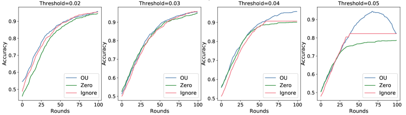
Figure 2: Accuracy of FedAvg with a fixed threshold communication strategy for varied values of the threshold. High thresholds prohibit convergence to an accurate model since all clients stop transmitting once their updates become smaller than the threshold.

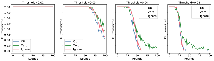
Figure 3: Per round communication of FedAvg with a fixed threshold communication strategy for varied thereshold values. Small thresholds fail to reduce communication, while high thresholds completely stop communication as training progresses thus leading to bad models.

We study the described FL systems in regards to the following main aspects of the client sampling problem: (i) communication efficiency vs. accuracy achieved by a client selection strategy; and (ii) the effects of different approaches to dealing with the clients that did not communicate their model updates to the server.

We first test our proposed client selection strategy and compare it with two baselines. In particular, we test our adaptive thresholding as well as its simpler variant wherein the threshold is fixed, and compare the results with those of the following baselines: (i) an approach where a fraction $q$ of $N$ clients is randomly dropped, with $q$ chosen to ensure a fair comparison with our thresholding schemes (specifically, $q$ is set equal to the average number of communicating clients per round in the thresholding scheme achieving the highest accuracy); and (ii) a non-restricted communication scheme where all clients communicate their model updates to the server.

Then we turn our attention to the policy for dealing with missing updates and consider two simple alternatives: (i) zero strategy, where the server replaces missing updates with zeros (essentially assuming that the model of a client which did not send its update is identical to the latest global model); and (ii) ignore, where the server averages only the updates it received. For notational convenience, we refer to our strategy for predicting missing updates as OU.

Note that in the experiments with EMNIST and Shakespeare datasets we fix hyperparameters as in the prior work Reddi et al. (2020), selecting $N=10$ clients at random in each round. All the models are trained for 100 rounds.

4.2.1 Fixed threshold

As described in Section 3, our proposed thresholding strategy relies on varying the value of the threshold according to the mean and standard deviation of the norms of the model updates. It is worth considering if a simpler scheme employing a fixed threshold might suffice. First, note that for the fixed threshold strategy OU client selection outperforms competing methods. Specifically, we observe in two right-most plots in Fig 2 that zero and ignore strategies stagnate and tend to converge slower than the OU strategy. However, using a fixed threshold fails to provide accurate yet communication-efficient FL systems. First, treating threshold as a hyperparameter adds a layer of complexity to the system design problem since different values of the threshold may lead to very different results, as observed in Fig 2. Tuning the threshold would go against the objective of reducing communication since a large number of rounds might be needed to facilitate the tuning. Finally, we observe that fixing the threshold to small values fails to reduce communication (left-most plot in Fig 3) while setting it to large values leads to inaccurate models (right-most plot in Fig 2).

4.2.2 Evaluation of the system end-to-end

We now evaluate our adaptive thresholding with OU estimation and compare it with the random selection strategy. In both contexts, random and thresholding, we perform OU, zero, and ignore estimation strategies, both on EMNIST and Shakespeare datasets. We use a full communication strategy as a baseline for accuracy.

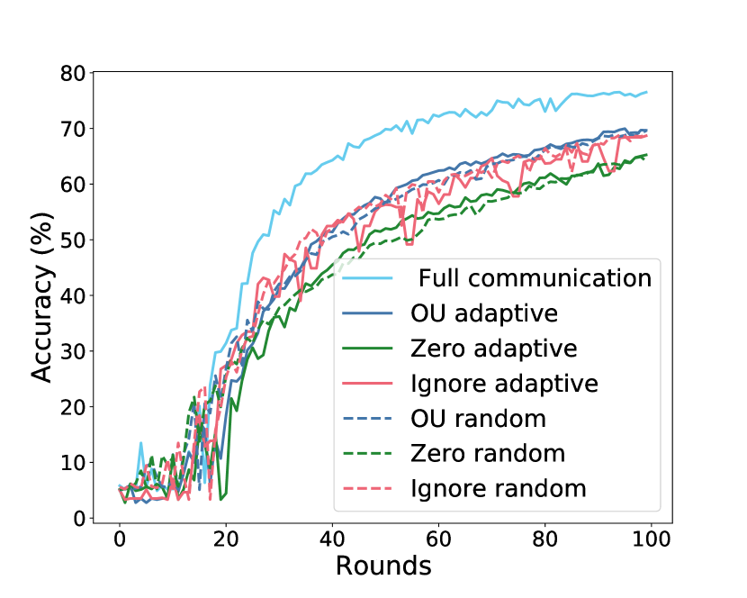
(a) Test accuracy of EMNIST CNN.

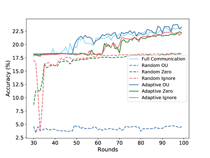
(b) Test accuracy of Shakespeare RNN.

Figure 4: Model accuracy on synthetic logistic regression, EMNIST, and Shakespeare. The OU client sampling strategy consistently outperforms the competing methods.

Accuracy.

In Fig 4, we plot the test accuracy progression during training for all combinations of random/adaptive selection and the three estimation strategies, namely OU, zero, and ignore, both on EMNIST and Shakespeare datasets. We observe that the OU estimation is consistently better than the other strategies. Ignoring updates also achieves high accuracy, although it experiences a significantly more unstable convergence. Finally, zero strategy achieves the worst performance. We notice that the approaches which take into account missing updates and replace them with an estimate, OU and zero, help smooth the training process. However, by zeroing out clients’ updates convergence is considerably slowed down on both datasets. On the other hand, OU is able to incorporate missing updates without rendering the convergence unstable. In both cases, the OU strategy achieves the best final accuracy; for the task involving Shakespeare dataset, OU even achieves better accuracy than the full-communication baseline scheme.

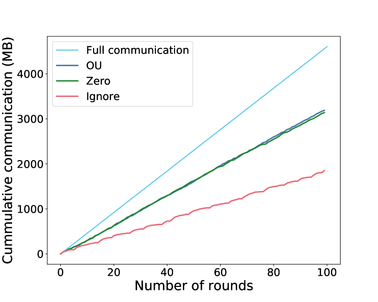
(a) EMNIST CNN.

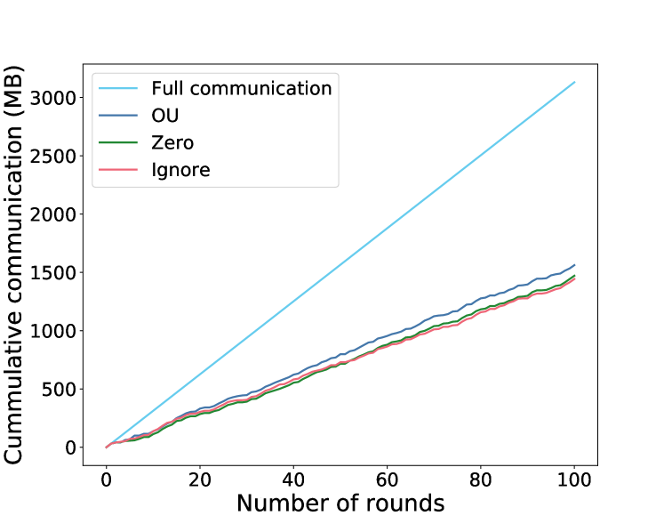
(b) Shakespeare RNN.

Figure 5: Cumulative communication of each system during training measured in total KBs sent. Ignore strategy saves much more communication in the case of EMNIST CNN but does so at the expense of accuracy.

Communication savings.

As shown in Fig 5, our thresholding with the OU sampling and estimation requires smaller amount of communication to achieve accuracy comparable to the baseline (i.e., to the scheme using updates of all clients). The zero estimation strategy has similar communication savings to OU in all cases, but with slower convergence rates and inferior final accuracy. Among all strategies, the ignore strategy achieves the highest communication savings but is ultimately not capable of matching the accuracy of the OU method. This lower communication rate of the ignore strategy is due to the fact that by ignoring certain clients, they will continue to have high norm value in the subsequent iterations, which further inflates the threshold and leads to even fewer clients in the next round. We further elaborate on this in the supplementary (Sec B.5).

While randomly dropping clients trivially achieves low communication rate (by definition equivalent to its adaptive estimation counterpart in each case), the random client selection scheme suffers from a deterioration in accuracy in heterogeneous and non-convex settings. In non-homogeneous, non-convex settings, estimating the true gradient from a subset of clients is much harder, and thus randomly dropping clients slows down the convergence. It is also in part consequence of dropping too many clients near the optimum where gradient norms might become smaller. Our adaptive thresholding strategy overcomes aforementioned problems by changing the threshold in each round based on the clients’ update norms. In the random setting, we observe that ignoring or zeroing updates is better, which accentuates the coupling of our thresholding and estimation strategies: by thresholding and using the MSE estimator we optimally incorporate the missing clients.

Our results demonstrate that the level of accuracy in FL can be maintained, or even outperformed, while reducing communication by using a smaller number of clients; however, these clients have to be carefully selected, and their updates have to be carefully incorporated in the new model.

The results in Table 2 suggest that while there is no single method which is uniformly superior in exploring accuracy-communication trade-offs, the thresholding strategies are an efficient way of subselecting clients without a significant deterioration of accuracy.

Table 2: Accuracy and communication cost of communication-reduction strategies in EMNIST and Shakespeare dataset experiment.

	Accuracy		Overall		Communication
	(%)		comm. (Gb)		used (%)
Dataset	EMNIST	Shakespeare	EMNIST	Shakespeare	EMNIST	Shakespeare
Baseline	76.51	22.86	4.5	3.1	100	100
Adaptive OU	69.67	23.3	3.15	1.53	70	49.9
Adaptive zero	65.25	22.18	3.01	1.44	68.9	47
Adaptive ignore	68.69	22.23	1.85	1.41	41.1	46.1
Random OU	69.58	4.56	3.16	1.46	70.34	47.9
Random zero	64.11	18.22	3.17	1.45	70.6	47.3
Random ignore	68.91	18.06	1.75	1.39	38.9	45.4

5 Conclusion

In this paper, we propose a novel approach to reducing communication rates in FL by judiciously subselecting clients instead of relying on traditional compression strategies. A parallel between OU processes and SGD suggests strategies for identifying clients whose updates are informative and therefore should be communicated to the server. Furthermore, utilizing this connection leads to an estimator for missing client model updates that can be calculated at the server using the previous updates. This estimation helps maintain and even improve the accuracy of the baseline scheme, while cutting communication by up to 50%. Experimental results demonstrate efficacy of the proposed methods in various settings. Moreover, our approach can be combined with compression strategies to lower the communication rates even further.

The proposed client selection protocol based on thresholding is theoretically justified by the existing results on optimal OU process sampling. Future work involves combining the methods proposed in this paper with the techniques that attempt to reduce communication burden by sparsifying transmitted information.

Appendix A Background details

A.1 Federated Averaging algorithm

For convenience and completeness, we here provide FedAvg, the baseline federated learning algorithm proposed in McMahan et al. [2017].

1

Input: $K$ clients, $B$ is the local minibatch size,$E$ is the number of local epochs, and $\eta$ is the learning rate.

Output: Global model $w$

2 initialize $w_{0}$;

3 for t=1,2,… do

4       $m\leftarrow\max(CK,1)$ ;

5       $S_{t}\leftarrow$ random set of $m$ clients ;

6       for  $k\in S_{t}$ in parallel do

7             $w^{k}_{t+1}\leftarrow$ ClientUpdate($k,w_{t}$) ;

8            

9       end for

10      $w_{t+1}\leftarrow\sum_{k=1}^{K}\frac{n_{k}}{n}w_{t+1}^{k}$ ;

11      

12 end for

13Clients execute: ;

14 ClientUpdate($k,w$) : Run on client $k$ ;

15 $\mathcal{B}\leftarrow$ split data $\mathcal{P}_{k}$ into batches of size $B$ ;

16 for $i=1,...,E$ do

17       for $b\in\mathcal{B}$ do

18             $w\leftarrow w-\eta\nabla\ell(w,b)$ ;

19            

20       end for

21      

22 end for

23return $w$ to server ;

Algorithm 4 FederatedAveraging McMahan et al. [2017]

Appendix B Experimental Details

B.1 Numerical illustration of SGD: Aptness of the OU process model

To illustrate the aptness of using OU process for modeling sequences of weights/parameters during SGD, we performed a simple experiment on the Fashion MNIST dataset Xiao et al. [2017]. This dataset consists of 60,000 training images and 10,000 test examples; each sample is a 28x28 image, belonging to one out of 10 categories. No user or id information is available.

We train a feed forward neural network with a single hidden layer consisting of 128 units, ReLU activation, and a softmax output layer. We train the model for 5 epochs with the batch size set to 100, for a final test accuracy of 84%, when the model saturates.

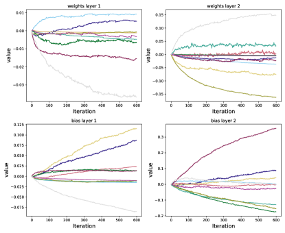
Figure 6: Parameter drift when retuning the model with new data. The weights follow trajectories reminiscent of the OU process sample paths.

In Fig 6 we show the trajectories of individual weights $w^{i}$ randomly selected from each layer (we plot the trajectories after centering by setting $w^{i}_{0}=0$). Similar to sample paths of an OU process, all trajectories in Fig 1 ultimately deviate towards a mean where they stabilize.

B.2 Datasets

The datasets used for benchmarking and model validation experiments are: (i) EMNIST dataset, a reprocessed version of the original MNIST dataset where each image is linked to its original writer, providing a non-i.i.d. natural distribution and allowing us to emulate an FL setting; and (ii) Shakespeare dataset, a language modelling dataset with questions and answers collected from users. Size of the datasets is summarized in the table below.

Table 3: Datasets

Dataset	Users	Samples
EMNIST	3.4 K	60 K
Shakespeare	715	16 K

B.3 Models

The ML architectures that we used are presented in Tables 1-2 below.

EMNIST CR

We train a convolutional neural network with the following architecture: two 5x5 convolution layers, with 32 and 64 channels respectively, interleaved with 2x2 max-pooling, a dense layer with 512 neurons with ReLU activation and a 10 unit softmax output layer. The network has a total of 1,663,370 parameters. At each round, 50 clients are uniformly selected to update the model. Each client locally trains for $E=20$ epochs using stochastic gradient descent (SGD) with a batch size of $B=10$.

Table 4: EMNIST digit recognition convolutional model architecture

Layer	Output	# Trainable parameters	Activation	Hyperparameters
Input	(28,28,1)
Conv2d	(26,26,32)	320	ReLU	kernel size = 3; strides(1,1)
Conv2d	(24,24,64)	18496		kernel size = 3; strides(1,1)
MaxPool2d	(12,12,64)	0		pool size= (2, 2)
Dropout	(12,12,64)	0		p=0.25
Flatten	9216	0
Dense	128	1179776
Dropout	128	0		p=0.5
Dense	62	7998	Softmax
Total		1,206,590

Shakespeare

We train a recursive neural network for the next character prediction that first embeds characters into an 8-dimensional space, followed by 2 LSTMs and finally a dense layer. The architecture is presented in Table 5.

Table 5: Shakespeare next character prediction model architecture

Layer	Output	# Trainable parameters	Activation
Input	80
Embedding	(80,8)	720
LSTM	(80,256)	271360
LSTM	(80,256)	525312
Dense	(80,90)	23130	Softmax
Total		4,050,748

B.4 Number of clients

Recall that when a new round starts, the server samples a fixed predetermined number $N$ of clients. As one would expect, increasing $N$ leads to improvement of accuracy of all the methods considered. We test how the performance vary with $N$ and show that our method consistently outperforms all the other strategies (see Table 7).

Table 6: Accuracy (%) on Shakespeare after $120$ rounds, with varying number of initial clients $N$

Method	Ada. OU	Ada. ignore	Ada. zero	Random OU	Random ignore	Random zero	Full comm.
N=10	23.3	22.22	22.18	4.98	18.05	18.22	22.8
N=20	23.96	23.37	23.06	0.0	20.57	18.26	23.55
N=50	25.17	24.31	24.78	24.51	21.24	21.03	26.63

Table 7: Communication rate (%) on Shakespeare with varying number of initial clients $N$

Method	Ada. OU	Ada. ignore	Ada. zero
N=10	46.6	46.02	47.3
N=20	47.43	47.14	47.98
N=50	48.95	48.93	49.13

B.5 Comparing thresholds across strategies

Assume adaptive thresholding schemes where a threshold is re-computed in each round based on statistics of the norms of the updates of participating clients (see line 12 in Algorithm 1); we empirically study thresholds generated by different strategies and the resulting communication rates. As expected, a strategy has an effect on the distribution of the magnitudes of the updates, leading to different thresholds and varied communication savings. In particular, in Fig 5 we observe that while OU and zero utilize similar levels of communication, ignore achieves more savings; this is particularly pronounced on EMNIST.

In Fig 7 we show the progression of thresholds for each strategy and in Table 8 we display the mean and variance of threshold across rounds. We observe the instability of ignore: by ignoring certain clients, the global model becomes inadequate for this group of clients; consequently, this estimation strategy may lead to larger future updates of those clients. The thresholds may take on larger values as well while, at the same time, experiencing an increased variance that may drive the threshold in some rounds to 0 (or to negative values which simply means that all clients transmit). OU and zero have a significantly more stable schedule of thresholds leading to smoother behavior of the magnitudes of model update norms; clearly, such benefits stem from incorporating estimates of the missing client updates in the computation of the next global model.

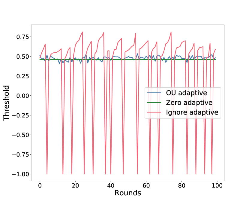
(a) Threshold EMNIST CNN.

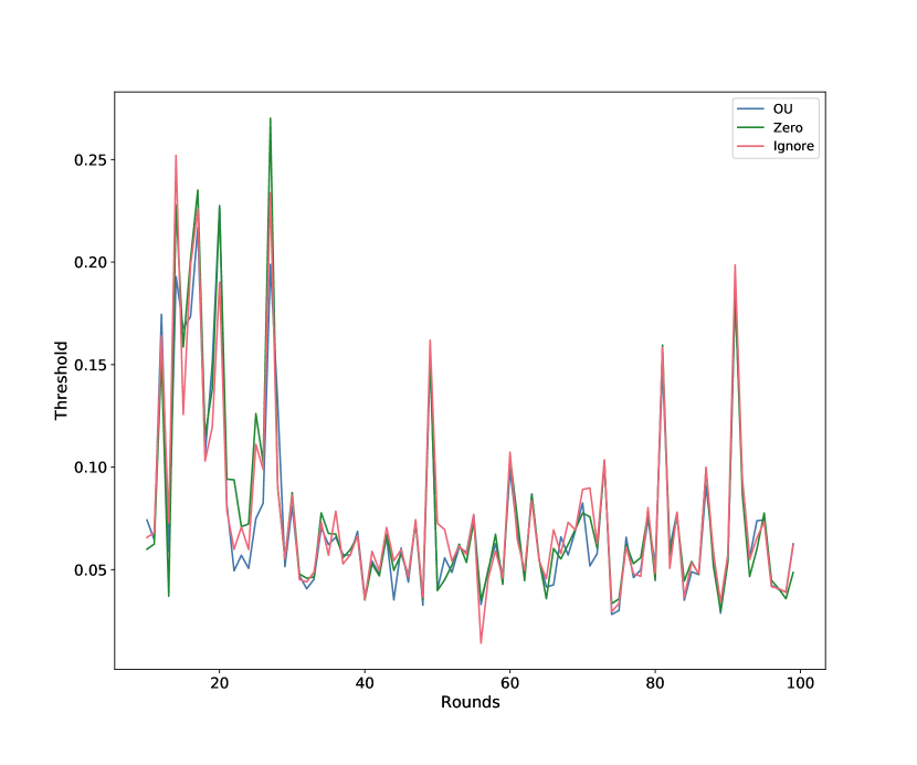
(b) Threshold of Shakespeare RNN.

Figure 7: Threshold values across rounds for different strategies.

Table 8: Mean threshold values across rounds.

	EMNIST	Shakespeare
OU	0.476 $\pm$ 0.03	0.746
Zero	0.459 $\pm$ 0.0	0.776
Ignore	0.515 $\pm$ 0.24	0.775

References

- Abadi et al. (2016) M. Abadi, A. Chu, I. Goodfellow, H. B. McMahan, I. Mironov, K. Talwar, and L. Zhang. Deep learning with differential privacy. pages 308–318. ACM, 2016.
- Acharya et al. (2018) J. Acharya, C. L. Canonne, and H. Tyagi. Inference under information constraints i: Lower bounds from chi-square contraction. arXiv preprint arXiv:1812.11476, 2018.
- Aghasi et al. (2016) A. Aghasi, N. Nguyen, and J. Romberg. Net-trim: A layer-wise convex pruning of deep neural networks. arXiv preprint arXiv:1611.05162, 2, 2016.
- Alistarh et al. (2017) D. Alistarh, D. Grubic, J. Li, R. Tomioka, and M. Vojnovic. Qsgd: Communication-efficient sgd via gradient quantization and encoding. In Advances in Neural Information Processing Systems, pages 1709–1720, 2017.
- Amin et al. (2019) K. Amin, A. Kulesza, A. Munoz, and S. Vassilvtiskii. Bounding user contributions: A bias-variance trade-off in differential privacy. In K. Chaudhuri and R. Salakhutdinov, editors, Proceedings of the 36th International Conference on Machine Learning, volume 97 of Proceedings of Machine Learning Research, pages 263–271, Long Beach, California, USA, 09–15 Jun 2019. PMLR. URL http://proceedings.mlr.press/v97/amin19a.html.
- Bagdasaryan et al. (2018) E. Bagdasaryan, A. Veit, Y. Hua, D. Estrin, and V. Shmatikov. How to backdoor federated learning. arXiv preprint arXiv:1807.00459, 2018.
- Balcan et al. (2012) M. F. Balcan, A. Blum, S. Fine, and Y. Mansour. Distributed learning, communication complexity and privacy. In Conference on Learning Theory, pages 26–1, 2012.
- Barnes et al. (2019) L. P. Barnes, Y. Han, and A. Ozgur. Learning distributions from their samples under communication constraints. arXiv preprint arXiv:1902.02890, 2019.
- Bhagoji et al. (2018) A. N. Bhagoji, S. Chakraborty, P. Mittal, and S. Calo. Analyzing federated learning through an adversarial lens. arXiv preprint arXiv:1811.12470, 2018.
- Blanc et al. (2019) G. Blanc, N. Gupta, G. Valiant, and P. Valiant. Implicit regularization for deep neural networks driven by an ornstein-uhlenbeck like process. arXiv preprint arXiv:1904.09080, 2019.
- Bommannavar and Başar (2008) P. A. Bommannavar and T. Başar. Optimal estimation over channels with limits on usage. IFAC Proceedings Volumes, 41(2):6632–6637, 2008.
- Bonawitz et al. (2016) K. Bonawitz, V. Ivanov, B. Kreuter, A. Marcedone, H. B. McMahan, S. Patel, D. Ramage, A. Segal, and K. Seth. Practical secure aggregation for federated learning on user-held data. arXiv preprint arXiv:1611.04482, 2016.
- Boyd et al. (2011) S. Boyd, N. Parikh, E. Chu, B. Peleato, and J. Eckstein. Distributed optimization and statistical learning via the alternating direction method of multipliers. Foundations and Trends® in Machine learning, 3(1):1–122, 2011.
- Braverman et al. (2016) M. Braverman, A. Garg, T. Ma, H. L. Nguyen, and D. P. Woodruff. Communication lower bounds for statistical estimation problems via a distributed data processing inequality. In Proceedings of the forty-eighth annual ACM symposium on Theory of Computing, pages 1011–1020, 2016.
- Caldas et al. (2018) S. Caldas, J. Konečny, H. B. McMahan, and A. Talwalkar. Expanding the reach of federated learning by reducing client resource requirements. arXiv preprint arXiv:1812.07210, 2018.
- Chen et al. (2018) T. Chen, G. Giannakis, T. Sun, and W. Yin. Lag: Lazily aggregated gradient for communication-efficient distributed learning. In Advances in Neural Information Processing Systems, pages 5050–5060, 2018.
- Cho et al. (2020) Y. J. Cho, J. Wang, and G. Joshi. Client selection in federated learning: Convergence analysis and power-of-choice selection strategies. arXiv preprint arXiv:2010.01243, 2020.
- Cohen et al. (2017) G. Cohen, S. Afshar, J. Tapson, and A. Van Schaik. Emnist: Extending mnist to handwritten letters. In 2017 International Joint Conference on Neural Networks (IJCNN), pages 2921–2926. IEEE, 2017.
- Courbariaux et al. (2015) M. Courbariaux, Y. Bengio, and J.-P. David. Binaryconnect: Training deep neural networks with binary weights during propagations. In Advances in neural information processing systems, pages 3123–3131, 2015.
- Dong et al. (2017) X. Dong, S. Chen, and S. Pan. Learning to prune deep neural networks via layer-wise optimal brain surgeon. In Advances in Neural Information Processing Systems, pages 4857–4867, 2017.
- Duchi et al. (2011) J. C. Duchi, A. Agarwal, and M. J. Wainwright. Dual averaging for distributed optimization: Convergence analysis and network scaling. IEEE Transactions on Automatic control, 57(3):592–606, 2011.
- Evans et al. (1994) L. T. Evans, S. P. Keef, and J. Okunev. Modelling real interest rates. Journal of banking & finance, 18(1):153–165, 1994.
- Geyer et al. (2017) R. C. Geyer, T. Klein, and M. Nabi. Differentially private federated learning: A client level perspective. arXiv preprint arXiv:1712.07557, 2017.
- Guo and Kostina (2020) N. Guo and V. Kostina. Optimal causal rate-constrained sampling for a class of continuous markov processes. arXiv preprint arXiv:2002.01581, 2020.
- Han et al. (2015) S. Han, H. Mao, and W. J. Dally. Deep compression: Compressing deep neural networks with pruning, trained quantization and huffman coding. arXiv preprint arXiv:1510.00149, 2015.
- Han et al. (2018) Y. Han, A. Özgür, and T. Weissman. Geometric lower bounds for distributed parameter estimation under communication constraints. arXiv preprint arXiv:1802.08417, 2018.
- Horvath et al. (2019) S. Horvath, C.-Y. Ho, L. Horvath, A. N. Sahu, M. Canini, and P. Richtarik. Natural compression for distributed deep learning. arXiv preprint arXiv:1905.10988, 2019.
- Hsieh et al. (2017) K. Hsieh, A. Harlap, N. Vijaykumar, D. Konomis, G. R. Ganger, P. B. Gibbons, and O. Mutlu. Gaia: Geo-distributed machine learning approaching LAN speeds. In 14th USENIX Symposium on Networked Systems Design and Implementation (NSDI 17), pages 629–647, 2017.
- Imer and Basar (2005) O. C. Imer and T. Basar. Optimal estimation with limited measurements. In Proceedings of the 44th IEEE Conference on Decision and Control, pages 1029–1034. IEEE, 2005.
- Kairouz et al. (2019) P. Kairouz, H. B. McMahan, B. Avent, A. Bellet, M. Bennis, A. N. Bhagoji, K. Bonawitz, Z. Charles, G. Cormode, R. Cummings, et al. Advances and open problems in federated learning. arXiv preprint arXiv:1912.04977, 2019.
- Konečnỳ and Richtárik (2018) J. Konečnỳ and P. Richtárik. Randomized distributed mean estimation: Accuracy vs. communication. Frontiers in Applied Mathematics and Statistics, 4:62, 2018.
- Konečnỳ et al. (2016) J. Konečnỳ, H. B. McMahan, F. X. Yu, P. Richtárik, A. T. Suresh, and D. Bacon. Federated learning: Strategies for improving communication efficiency. arXiv preprint arXiv:1610.05492, 2016.
- Lemons and Langevin (2002) D. S. Lemons and P. Langevin. An introduction to stochastic processes in physics. JHU Press, 2002.
- Li et al. (2018) T. Li, L. Liu, A. Kyrillidis, and C. Caramanis. Statistical inference using sgd. In Thirty-Second AAAI Conference on Artificial Intelligence, 2018.
- Lin et al. (2016) D. Lin, S. Talathi, and S. Annapureddy. Fixed point quantization of deep convolutional networks. In International Conference on Machine Learning, pages 2849–2858, 2016.
- Liptser and Shiryaev (2013) R. S. Liptser and A. N. Shiryaev. Statistics of random processes II: Applications, volume 6. Springer Science & Business Media, 2013.
- Mandt et al. (2016) S. Mandt, M. Hoffman, and D. Blei. A variational analysis of stochastic gradient algorithms. In International conference on machine learning, pages 354–363, 2016.
- McMahan et al. (2017) B. McMahan, E. Moore, D. Ramage, S. Hampson, and B. A. y Arcas. Communication-Efficient Learning of Deep Networks from Decentralized Data. In A. Singh and J. Zhu, editors, Proceedings of the 20th International Conference on Artificial Intelligence and Statistics, volume 54 of Proceedings of Machine Learning Research, pages 1273–1282, Fort Lauderdale, FL, USA, 20–22 Apr 2017. PMLR. URL http://proceedings.mlr.press/v54/mcmahan17a.html.
- McMahan et al. (2018) H. B. McMahan, G. Andrew, U. Erlingsson, S. Chien, I. Mironov, N. Papernot, and P. Kairouz. A general approach to adding differential privacy to iterative training procedures. arXiv preprint arXiv:1812.06210, 2018.
- Nar and Başar (2014) K. Nar and T. Başar. Sampling multidimensional wiener processes. In 53rd IEEE Conference on Decision and Control, pages 3426–3431, Dec 2014. doi: 10.1109/CDC.2014.7039920.
- Nayyar et al. (2013) A. Nayyar, T. Başar, D. Teneketzis, and V. V. Veeravalli. Optimal strategies for communication and remote estimation with an energy harvesting sensor. IEEE Transactions on Automatic Control, 58(9):2246–2260, 2013.
- Nishio and Yonetani (2019) T. Nishio and R. Yonetani. Client selection for federated learning with heterogeneous resources in mobile edge. In ICC 2019 - 2019 IEEE International Conference on Communications (ICC), pages 1–7, 2019.
- Oktay et al. (2019) D. Oktay, J. Ballé, S. Singh, and A. Shrivastava. Model compression by entropy penalized reparameterization. arXiv preprint arXiv:1906.06624, 2019.
- Ornee and Sun (2019) T. Z. Ornee and Y. Sun. Sampling for remote estimation through queues: Age of information and beyond. arXiv preprint arXiv:1902.03552, 2019.
- Rabi et al. (2012) M. Rabi, G. V. Moustakides, and J. S. Baras. Adaptive sampling for linear state estimation. SIAM Journal on Control and Optimization, 50(2):672–702, 2012.
- Reddi et al. (2020) S. Reddi, Z. Charles, M. Zaheer, Z. Garrett, K. Rush, J. Konečnỳ, S. Kumar, and H. B. McMahan. Adaptive federated optimization. arXiv preprint arXiv:2003.00295, 2020.
- Ribero et al. (2020) M. Ribero, J. Henderson, S. Williamson, and H. Vikalo. Federating recommendations using differentially private prototypes. arXiv preprint arXiv:2003.00602, 2020.
- Ricciardi and Sacerdote (1979) L. M. Ricciardi and L. Sacerdote. The ornstein-uhlenbeck process as a model for neuronal activity. Biological cybernetics, 35(1):1–9, 1979.
- Rohlfs et al. (2014) R. V. Rohlfs, P. Harrigan, and R. Nielsen. Modeling gene expression evolution with an extended ornstein–uhlenbeck process accounting for within-species variation. Molecular biology and evolution, 31(1):201–211, 2014.
- Shao and Tu (2012) J. Shao and D. Tu. The jackknife and bootstrap. Springer Science & Business Media, 2012.
- Simonyan and Zisserman (2014) K. Simonyan and A. Zisserman. Very deep convolutional networks for large-scale image recognition. arXiv preprint arXiv:1409.1556, 2014.
- Singh et al. (2019) N. Singh, D. Data, J. George, and S. Diggavi. Sparq-sgd: Event-triggered and compressed communication in decentralized stochastic optimization. arXiv preprint arXiv:1910.14280, 2019.
- Siu-tang and Xin (2015) L. T. Siu-tang and L. Xin. Optimal mean reversion trading: Mathematical analysis and practical applications, volume 1. World Scientific, 2015.
- Smith et al. (2017) V. Smith, C.-K. Chiang, M. Sanjabi, and A. S. Talwalkar. Federated multi-task learning. In Advances in Neural Information Processing Systems, pages 4424–4434, 2017.
- Stein and Stein (1991) E. M. Stein and J. C. Stein. Stock price distributions with stochastic volatility: an analytic approach. The review of financial studies, 4(4):727–752, 1991.
- Sun et al. (2017) Y. Sun, Y. Polyanskiy, and E. Uysal-Biyikoglu. Remote estimation of the wiener process over a channel with random delay. In 2017 IEEE International Symposium on Information Theory (ISIT), pages 321–325. IEEE, 2017.
- Suresh et al. (2017) A. T. Suresh, F. X. Yu, S. Kumar, and H. B. McMahan. Distributed mean estimation with limited communication. In Proceedings of the 34th International Conference on Machine Learning-Volume 70, pages 3329–3337. JMLR. org, 2017.
- Tang et al. (2019) H. Tang, X. Lian, T. Zhang, and J. Liu. Doublesqueeze: Parallel stochastic gradient descent with double-pass error-compensated compression. arXiv preprint arXiv:1905.05957, 2019.
- Wang (2017) Y. Wang. Asymptotic analysis via stochastic differential equations of gradient descent algorithms in statistical and computational paradigms. arXiv preprint arXiv:1711.09514, 2017.
- Wu et al. (2017) X. Wu, F. Li, A. Kumar, K. Chaudhuri, S. Jha, and J. Naughton. Bolt-on differential privacy for scalable stochastic gradient descent-based analytics. pages 1307–1322. ACM, 2017.
- Xiao et al. (2017) H. Xiao, K. Rasul, and R. Vollgraf. Fashion-mnist: a novel image dataset for benchmarking machine learning algorithms, 2017.
- Zhang et al. (2013a) Y. Zhang, J. Duchi, M. I. Jordan, and M. J. Wainwright. Information-theoretic lower bounds for distributed statistical estimation with communication constraints. In Advances in Neural Information Processing Systems, pages 2328–2336, 2013a.
- Zhang et al. (2013b) Y. Zhang, J. C. Duchi, and M. J. Wainwright. Communication-efficient algorithms for statistical optimization. The Journal of Machine Learning Research, 14(1):3321–3363, 2013b.
- Zhu and Gupta (2017) M. Zhu and S. Gupta. To prune, or not to prune: exploring the efficacy of pruning for model compression. arXiv preprint arXiv:1710.01878, 2017.