Effect of quantum resonances on local temperature in nonequilibrium open systems

Abstract

Measuring local temperatures of open systems out of equilibrium is emerging as a novel approach to study the local thermodynamic properties of nanosystems. An operational protocol has been proposed to determine the local temperature by coupling a probe to the system and then minimizing the perturbation to a certain local observable of the probed system. In this paper, we first show that such a local temperature is unique for a single quantum impurity and the given local observable. We then extend this protocol to open systems consisting of multiple quantum impurities by proposing a local minimal perturbation condition (LMPC). The influence of quantum resonances on the local temperature is elucidated by both analytic and numerical results. In particular, we demonstrate that quantum resonances may give rise to strong oscillations of the local temperature along a multi-impurity chain under a thermal bias.

I INTRODUCTION

Local temperatures of systems out of equilibriumZhang2019local are of fundamental importance in many sub-fields of modern science, including physics,Hof09779 ; menges2013thermal ; Men1610874 ; Inu184304 chemistryLee13209 ; Cui18122 ; Nov19016806 and biology.Zei04871 ; Kuc1354 ; He1626737 With the development of high-resolution thermometric techniques,Sadat2012High ; mecklenburg2015Nanoscale ; Men1610874 the measurement of local temperature distributions in nonequilibrium nanoscopic systems has been realized, such as in graphene-metal contacts,Gro11287 aluminum nanowires,mecklenburg2015Nanoscale and two-dimensional metallic films.Gurrum2005Scanning

A nonequilibrium system under an external driving source, such as a bias voltage or a thermal gradient, often possesses a local temperature somewhat higher than the background temperature.di2008electrical Such a local heating effect usually originates from the electronic and phononic excitations occurring in the system and has significant influence on some physical propertiesLiu2015Density and processes.Hua061240 ; huang2007local ; Kim14203107 ; Thi15854 ; Ivo16014301 ; Idr18095901

Theoretically, the concept of temperature has been extended from equilibrium systems to local subregions of nonequilibrium systems.scovil1959three ; curzon1975efficiency ; lieb1999physics ; allahverdyan2001breakdown ; casas2003temperature ; kieu2004second ; bustamante2005nonequilibrium ; horhammer2008information ; bergfield2009many ; levy2012quantum ; horodecki2013fundamental ; skrzypczyk2014work ; hardal2015superradiant ; clos2016time ; puglisi2017temperature ; marcantoni2017entropy ; monsel2018autonomous ; bialas2019quantum ; Zhang2019local Ideally, the definition of local temperature should be universal (so that it can be applied to as many nonequilibrium situations as possible), unique (so that it yields one and only one value of temperature), operationally feasible (so that it can be measured experimentally), and has the correct asymptotic limit (so that it retrieves the thermodynamic temperature as the system approaches an equilibrium state).Zhang2019local

For instance, Engquist and Anderson have proposed a procedure for measuring the local temperature and local chemical potential of nonequilibrium systems.engquist1981definition In their definition, the local temperature and local chemical potential are measured, respectively, by a thermometer in thermal equilibrium with the system of interest and a potentiometer in electrical equilibrium with the system. Later, Bergfield and Stafford et al. pointed out that the above definition implicitly ignores thermoelectric effects and is nonunique.bergfield2013probing ; Bergfield2014Thermoelectric ; shastry2020scanning They have proposed a definition in which the local temperature and local chemical potential of a nonequilibrium system are determined simultaneously.bergfield2013probing ; bergfield2015tunable ; shastry2016temperature ; shastry2020scanning In their definition, a probe which plays the roles of both potentiometer and thermometer is weakly coupled to the nonequilibrium system of interest. By varying the temperature ($T_{p}$) and chemical potential ($\mu_{p}$) of the probe until both the electric ($I_{p}$) and heat currents ($J_{p}$) flowing through the probe vanish, the local temperature ($T^{\ast}$) and local chemical potential ($\mu^{\ast}$) of the system are determined as $T^{\ast}=T_{p}$ and $\mu^{\ast}=\mu_{p}$, respectively. Such a condition is referred to as the zero current condition (ZCC).Zhang2019local

The ZCC-based definition has been used to investigate local temperatureMeair2014Local ; Bergfield2014Thermoelectric ; Shastry2015Cold ; Stafford2016Local ; Stafford2017Local and local electrochemical potential distributionbevan2014first ; morr2016crossover ; morr2017scanning in nanosystems out of equilibrium.caso2010local ; caso2011local ; caso2012defining It was found that the local temperature ($T^{\ast,{\rm ZCC}}$) exhibits an oscillatory behavior in nanowires,caso2011local conjugated organic moleculesbergfield2013probing and graphene sheets.bergfield2015tunable Such oscillations originate from the emergence of quantum coherence as the size of the system reduces to be comparable to or even smaller than the mean free path of electrons.dubi2009thermoelectric Consequently, the classical Fourier’s law is strongly violated.michel2003fourier ; dhar2008heat ; roy2008crossover ; yang2010violation ; Zhang2019local Although it has been demonstrateddubi2009thermoelectric ; caso2010local ; caso2011local ; bergfield2013probing ; Meair2014Local ; bergfield2015tunable ; Inu184304 that quantum coherence and quantum interference effects could be captured by $T^{\ast,{\rm ZCC}}$, it was also shown that $T^{\ast,{\rm ZCC}}$ of a quantum dot experiences little change as the dot is tuned from an off-resonance region into a resonance region.ye2016thermodynamic Therefore, it remains unclear whether $T^{\ast,{\rm ZCC}}$ could reflect the emergence of sharp quantum resonances.

The ZCC-based definition has the advantage of yielding a unique value of local temperature for any nonequilibrium system,shastry2016temperature and it is applicable even in situations where local equilibrium states do not exist.Meair2014Local However, its experimental realization is rather challenging because of the difficulty in measuring the heat current through a nanosized sample without knowing its priori local temperature.Zhang2019local Recently, Shastry and co-workers have modified the ZCC-based protocol,shastry2020scanning and the new protocol does not require the measurement of heat current if the system obeys the Wiedemann-Franz law. However, the Wiedemann-Franz law is known to be violated by systems involving strong many-body interactionscrossno2016observation or low-energy quantum resonant states.Ye2014Thermopower

Alternatively, an operational protocol to determine the local temperature has been proposed based on a minimal-perturbation condition (MPC),dubi2009thermoelectric ; Ye2015local ; ye2016thermodynamic with which the local temperature ($T^{\ast,{\rm MPC}}$) is determined by tuning $T_{p}$ and $\mu_{p}$ of a weakly coupled probe until the perturbation caused by the probe to the system gets minimized.

Ideally, if the perturbation caused by the probe to the system can be nullified, any dissipation between the system and the probe, particularly the energy and particle flows, would vanish. In such cases, the MPC can be deemed as a generalization of the zeroth law, and it naturally leads to the ZCC; see the formal proof in Appendix A. Meanwhile, as a result of zero dissipation, any observable of the system preserves its intrinsic value as in the absence of the probe. However, in some occasions, such as when quantum resonances come into play,ye2016thermodynamic the influence of the probe cannot be fully suppressed. In the latter case, the MPC stands as an empirical principle which minimizes the dissipation between the system and the probe, while its thermodynamic meaning is less transparent. Because of the difficulty in measuring the heat current directly, in practice the dissipation is characterized by the particle current as well as the change of a certain system observable. The resulting MPC-based protocol has been applied to investigate local temperatures of strongly correlated quantum impurity systems.Ye2015local ; ye2016thermodynamic

Despite the effectiveness and feasibility of the MPC-based definition, there are still issues that remain unclear. Some of them are as follows: (i) Does the MPC predict a unique value of $T^{\ast}$? (ii) Why and how does $T^{\ast,{\rm MPC}}$ differ from $T^{\ast,{\rm ZCC}}$ in systems involving quantum resonances? (iii) So far the application of the MPC has been restricted to systems containing a single impurity. How do we extend the definition of $T^{\ast,{\rm MPC}}$ to multi-impurity systems? (iv) Do quantum resonances lead to any discernible feature in the distribution of local temperatures along a quantum wire?

This work aims at elucidating the above issues through theoretical analysis and numerical calculations. In particular, to address the last two questions, we propose a local minimal-perturbation condition (LMPC) by imposing explicitly the nonequilibrium-equilibrium correspondence relation. As a direct extension of the original MPC, the LMPC enables the determination of the local temperature and local chemical potential of each impurity in a multi-impurity system out of equilibrium.

The remainder of this paper is organized as follows. In Sec. II, we revisit the MPC protocol and discuss how to reach a unique prediction of the local temperature of a single quantum impurity. In Sec. III, we propose the LMPC-based definition of local temperature. As a numerical example we calculate the distribution of local temperatures along a quantum wire consisting of four impurities. Concluding remarks are given in Sec. IV.

II Effect of quantum resonances on local temperatures of single impurity systems

II.1 Quantum impurity systems

In the following, the Anderson impurity models (AIMs)anderson1961localized are adopted to describe the open systems. The total Hamiltonian of the system plus environment is

$$\hat{H}=\hat{H}_{\rm imp}+\hat{H}_{\rm lead}+\hat{H}_{\rm coup},$$ (1)

where the three terms on the right-hand side (RHS) represent the Hamiltonian of the impurities, the Hamiltonian of the leads which serve as the electron reservoirs and heat baths, and the Hamiltonian of the impurity-lead couplings, respectively.

We consider first a single impurity described by $\hat{H}_{\rm imp}=\epsilon_{d}\,\hat{n}+U\hat{n}_{\uparrow}\,\hat{n}_{\downarrow}$. Here, $\hat{n}=\sum_{s}\hat{n}_{s}=\sum_{s}\hat{a}^{\dagger}_{s}\,\hat{a}_{s}$, with $\hat{a}^{\dagger}_{s}$ ($\hat{a}_{s}$) creating (annihilating) an electron of spin $s$ on the impurity level $\epsilon_{d}$, and $U$ is the Coulomb interaction energy between the spin-up and spin-down electrons. $\hat{H}_{\rm lead}=\sum_{\alpha ks}\epsilon_{\alpha k}\,\hat{d}^{\dagger}_{\alpha ks}\,\hat{d}_{\alpha ks}$ and $\hat{H}_{\rm coup}=\sum_{\alpha ks}t_{\alpha k}\,\hat{a}^{\dagger}_{s}\,\hat{d}_{\alpha ks}+{\rm H.c.}$ describe the noninteracting leads and the impurity-lead coupling, respectively. Here, $\hat{d}^{\dagger}_{\alpha ks}(\hat{d}_{\alpha ks})$ creates (annihilates) a spin-$s$ electron on the $k$th orbital of the $\alpha$th lead, and $t_{\alpha k}$ is the coupling strength between the impurity level and the $k$th lead orbital.

To investigate the properties of the impurity, the hierarchical equations of motion (HEOM) approachTanimura1989Time ; jin2008exact ; li2012hierarchical ; Cui2019Highly ; Zhang2020Hierarchical ; Tanimura2020Numerically is employed, which takes the reduced density matrix of the impurity and a hierarchical set of auxiliary density operators as the basic variables. The HEOM theory is, in principle, formally exact, and its numerical outcomes are guaranteed to be quantitatively accurate if the results converge with respect to the truncation tier of the hierarchy ($L$).Ye16608 ; Han2018On For noninteracting impurities ($U=0$), the HEOM theory is formally equivalent to the nonequilibrium Green’s function (NEGF) formalism,jin2008exact and a low truncation tier of $L=2$ suffices to yield exact single-electron properties. For interacting AIMs ($U\neq 0$), while the analysis with the NEGF method is difficult because the self-energies due to electron-electron interaction cannot be expressed analytically, the HEOM approach can still yield accurate numerical results (usually with a truncation tier of $L>2$).Zheng2009Numerical ; zheng2013kondo ; Wang2013Hierarchical ; Ye2014Thermopower ; Hou2015Improving ; Ye2015local ; ye2016thermodynamic ; Wang2018Precise ; li2020molecular

In the framework of the HEOM, the influence of the noninteracting leads on the impurity is fully captured by the hybridization functions, $\Gamma_{\alpha}(\omega)\equiv\pi\sum_{k}|t_{\alpha k}|^{2}\delta(\omega-\epsilon_{\alpha k})$. For numerical convenience, a Lorentzian form of $\Gamma_{\alpha}(\omega)=\frac{\Delta_{\alpha}W_{\alpha}^{2}}{(\omega-\Omega_{\alpha})^{2}+W_{\alpha}^{2}}$ is adopted, where $\Delta_{\alpha}$ is the effective coupling strength between the impurity and the $\alpha$th lead, and $\Omega_{\alpha}$ and $W_{\alpha}$ are the band center and width of the $\alpha$th lead, respectively. We further set the band center at the chemical potential of the lead, i.e., $\Omega_{\alpha}=\mu_{\alpha}$. The chemical potential of the equilibrium composite system is set to the zero energy, i.e., $\mu^{\rm eq}=0$.

In the following, $\Delta_{p}$ (the subscript $p$ denotes the probe) is taken to be at least two orders of magnitude smaller than all the other $\Delta_{\alpha}$, and further reducing its value does not influence the resulting $T^{\ast}$ and $\mu^{\ast}$.Ye2015local Hereafter, we adopt the atomic units $e=\hbar=k_{\rm B}\equiv 1$, and $\Delta=\sum_{\alpha\neq p}\Delta_{\alpha}$ is taken as the unit of energy.

II.2 Minimal-perturbation condition

The MPC-based protocol is generally applicable to any quantum impurity system regardless of the specific form of the system Hamiltonian. Here, we consider the scenario that a single impurity is coupled to the left ($L$) and right ($R$) leads, whose background temperatures (chemical potentials) are $T_{L}$ and $T_{R}$ ($\mu_{L}$ and $\mu_{R}$), respectively. By coupling an external probe to the impurity, the local observable $O=\langle\hat{O}\rangle={\rm tr}(\hat{O}\rho)$ is subject to a perturbation of

$$\delta O_{p}=O_{p}(T_{p},\mu_{p})-O_{\rm ref}.$$ (2)

Here, $O_{p}(T_{p},\mu_{p})$ is the value of $O$ measured by setting the temperature and chemical potential of the coupled probe to $T_{p}$ and $\mu_{p}$, respectively. $O_{\rm ref}$ is the minimally perturbed value of $O$ which serves as reference for $O_{p}$. For a single-impurity system, $O_{\rm ref}$ is determined by

$$O_{\rm ref}=\zeta_{L}O_{p}(T_{L},\mu_{L})+\zeta_{R}O_{p}(T_{R},\mu_{R}),$$ (3)

where the coefficients $\zeta_{\alpha}$ ($\alpha=L$ and $R$) are acquired asYe2015local

$$\zeta_{\alpha}=1-\left|\frac{I_{p}(T_{\alpha},\mu_{\alpha})}{I_{p}(T_{L},\mu_{L})-I_{p}(T_{R},\mu_{R})}\right|.$$ (4)

Here, $I_{p}(T_{p},\mu_{p})$ is the electric current flowing into the probe with its temperature and chemical potential set to $T_{p}$ and $\mu_{p}$, respectively. For AIMs, $\zeta_{\alpha}=\frac{\Delta_{\alpha}}{\Delta_{L}+\Delta_{R}}$.

The local temperature $T^{\ast}$ and local chemical potential $\mu^{\ast}$ of the impurity are determined by

$$\left\{\begin{aligned} &{I_{p}(T^{\ast},\mu^{\ast})=0}\\ &(T^{\ast},\mu^{\ast})={\arg\min_{(T_{p},\mu_{p})}|\delta O_{p}(T_{p},\mu_{p})|}\end{aligned}\right..$$ (5)

In particular, if $\delta O_{p}=0$ is achievable by tuning $T_{p}$ and $\mu_{p}$, the MPC actually becomes the zero perturbation condition (ZPC). The definition of Eq. (5) does not involve the troublesome heat current, and all the involving quantities (e.g. $I_{p}$ and $O_{p}$) can be measured directly in experiments. Therefore, Eq. (5) provides an operational protocol for the determination of $T^{\ast}$ and $\mu^{\ast}$. In practice, such a protocol for the system under a bias voltage may be further simplified with a preset $\mu^{\ast}$ as follows,

$$\left\{\begin{aligned} &{\mu^{\ast}\approx\zeta_{L}\mu_{L}+\zeta_{R}\mu_{R}}\\ &{T^{\ast}=\arg\min_{T_{p}}|\delta O_{p}(T_{p},\mu^{\ast})|}\end{aligned}\right..$$ (6)

For a convenient and accurate measurement of $T^{\ast}$, the local observable $O$ should vary sensitively with $T_{p}$. In our previous works,Ye2015local ; ye2016thermodynamic the local magnetic and charge susceptibilities of the impurity, $\chi^{m}=\frac{\partial\langle\hat{m}_{z}\rangle}{\partial H_{z}}|_{H_{z}\rightarrow 0}$ and $\chi^{c}=-\frac{\partial\langle\hat{n}\rangle}{\partial\epsilon_{d}}$, respectively, have been chosen as the local observables. Here, $\hat{m}_{z}=\frac{1}{2}g\,\mu_{{}_{\rm B}}(\hat{n}_{\uparrow}-\hat{n}_{\downarrow})$ is the impurity magnetization operator, with $H_{z}$ being the local magnetic field, $g$ the electron gyromagnetic ratio, and $\mu_{{}_{\rm B}}$ the Bohr magneton. It has been shown that while $T^{\ast,{\rm MPC}}(\chi^{m})$ and $T^{\ast,{\rm MPC}}(\chi^{c})$ agree closely with each other in most cases, they do exhibit small discrepancy in the near-resonance (NR) region.ye2016thermodynamic

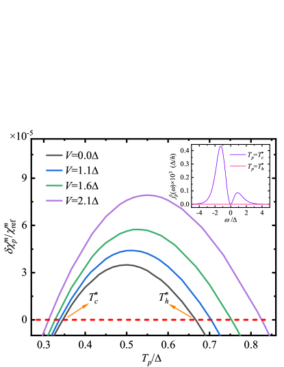
Figure 1: $\delta\chi^{m}_{p}/\chi^{m}_{\rm ref}$ as a function of $T_{p}$ for a single-impurity system under an antisymmetric bias voltage of $\mu_{R}=-\mu_{L}=V/2$. $T^{\ast}_{c}$ and $T^{\ast}_{h}$ are two temperatures which satisfy the ZPC of $\delta\chi^{m}_{p}=0$, as indicated by the horizontal line. The energetic parameters of the system are (in units of $\Delta$): $T_{L}=T_{R}=0.67$, $\epsilon_{d}=-3.33$, $\Delta_{L}=\Delta_{R}=0.5$, $U=2.5$, and $W_{L}=W_{R}=6.67$. The inset depicts the energy distribution of the heat current flowing into the probe [$j_{p}^{1}(\omega)$] at $T_{p}=T_{c}^{\ast}$ and $T_{p}=T_{h}^{\ast}$ under the zero bias, respectively. The detailed expression of $j_{p}^{1}(\omega)$ has been given in Ref. [Ye2015local, ], and $J_{p}=\int j_{p}^{1}(\omega)d\omega$.

In the following, we explore the uniqueness/nonuniqueness of the $T^{\ast,{\rm MPC}}$. First, we show that the MPC of Eq. (5) or Eq. (6) may give rise to multiple values of $T^{\ast}$ with a certain $O$. Figure 1 depicts the relative perturbation of local magnetic susceptibility, $\delta\chi^{m}_{p}/\chi_{\rm ref}^{m}$, as a function of $T_{p}$ for a single-impurity system under an antisymmetric bias voltage. From the first line of Eq. (6) we have $\mu^{\ast}=0$ since $\Delta_{L}=\Delta_{R}$. Meanwhile, it is intriguing to find that there are two temperatures that could satisfy the ZPC of $\delta\chi^{m}_{p}=0$, which are designated as $T^{\ast}_{c}$ and $T^{\ast}_{h}$ ($T^{\ast}_{c}<T^{\ast}_{h}$). Thus, the local temperature $T^{\ast,{\rm MPC}}$ appears to be nonunique. However, it is important to note that, as the bias voltage is reduced the whole system should evolve towards an equilibrium state. In particular, in the limit of $V\rightarrow 0$, $T^{\ast,{\rm MPC}}$ should recover the thermodynamic temperature of the equilibrium system, i.e., $T^{\ast,{\rm MPC}}=T_{L}=T_{R}$. In particular, as indicated by the inset of Fig. 1, the heat current through the probe ($J_{p}$) vanishes only at $T_{p}=T_{h}^{\ast}=T_{L}=T_{R}$, while it retains an appreciable value at $T_{p}=T_{c}^{\ast}$. It is thus evident that only $T^{\ast}_{h}$ achieves the correct asymptotic limit under the zero bias and recovers the zeroth law. Therefore, although the MPC of Eq. (6) has multiple solutions, because it does not explicitly examine the heat current, the $T^{\ast,{\rm MPC}}$ can still be uniquely determined for a given local observable $O$ by considering the asymptotic limit of the global equilibrium state.

II.3 Effect of quantum resonances on local temperature

We then explore the uniqueness/nonuniqueness of $T^{\ast,{\rm MPC}}$ associated with different local observables in the off-resonance, near-resonance, and resonance regions. To this end, we consider a noninteracting single-impurity system under an antisymmetric bias voltage. Figure 2 depicts the variation of $T^{\ast,{\rm MPC}}$ determined by Eq. (6) with the change of $\epsilon_{d}$. The displayed $T^{\ast,{\rm MPC}}$ are associated with the electron occupation number on the impurity $n=\langle\hat{n}\rangle$ or with the local charge susceptibility $\chi^{c}$. In both cases, we have $\mu^{\ast,{\rm MPC}}=0$ since $\Delta_{L}=\Delta_{R}$. For comparison, the $T^{\ast,{\rm ZCC}}$ versus $\epsilon_{d}$ are also shown in Fig. 2.

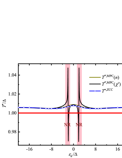
Figure 2: $T^{\ast,{\rm MPC}}(n)$, $T^{\ast,{\rm MPC}}(\chi^{c})$, and $T^{\ast,{\rm ZCC}}$ versus $\epsilon_{d}$ for a noninteracting single-impurity system under an antisymmetric bias voltage of $\mu_{R}=-\mu_{L}=V/2=0.2\Delta$. The energetic parameters of the system are (in units of $\Delta$): $T_{L}=T_{R}=1$, $U=0$, $\Delta_{L}=\Delta_{R}=0.5$, and $W_{L}=W_{R}=50$. The shaded areas represent the NR regions.

From Fig. 2, it is clear that $T^{\ast,{\rm ZCC}}$ and $T^{\ast,{\rm MPC}}(n)$ vary smoothly and coincide closely with each other over the whole range of $\epsilon_{d}$. In contrast, while the $T^{\ast,{\rm MPC}}(\chi^{c})$ agree well with the other two local temperatures in the off-resonance regions ($|\epsilon_{d}|$ is far away from the chemical potentials of leads), they exhibit strong oscillations in the NR regions. Such oscillations reflect the emergence of nonlocal excitations as a quantum resonant state begins to establish in the system.ye2016thermodynamic

To understand the quantitative agreement between $T^{\ast,{\rm MPC}}(n)$ and $T^{\ast,{\rm ZCC}}$ in Fig. 2, we carry out some theoretical analysis by using the NEGF method. In the wide-band limit ($W\rightarrow\infty$), the spin-$s$ component of the steady-state electric current flowing into the probe is

$$I_{ps} =-\frac{i}{\pi}\int d\omega\,\Gamma_{p}(\omega)\left\{G_{s}^{<}(\omega)+2if_{T_{p},\mu_{p}}(\omega)\,{\rm Im}[G^{r}_{s}(\omega)]\right\}$$

$$=\frac{2\Delta_{p}\Delta}{\Delta+\Delta_{p}}\int d\omega\,A_{s}(\omega)\,\big{[}\zeta_{L}f_{T_{L},\mu_{L}}(\omega)$$

$$\qquad\qquad\qquad+\zeta_{R}f_{T_{R},\mu_{R}}(\omega)-f_{T_{p},\mu_{p}(\omega)}\big{]},$$ (7)

and the electron occupation number on the impurity is

$$n =\sum_{s}n_{s}=\sum_{s}\frac{1}{2\pi i}\int d\omega\,G_{s}^{<}(\omega)$$

$$=\sum_{\alpha}\frac{\Delta_{\alpha}}{\Delta+\Delta_{p}}\int d\omega\,A(\omega)f_{T_{\alpha},\mu_{\alpha}}(\omega).$$ (8)

Here, $G_{s}^{r}(\omega)$ and $G_{s}^{<}(\omega)$ are the retarded and lesser single-electron Green’s functions of the impurity, respectively; $A(\omega)=\sum_{s}A_{s}(\omega)=-\frac{1}{\pi}\sum_{s}{\rm Im}[G_{s}^{r}(\omega)]$ is the spectral function of the impurity, and $f_{T_{\alpha},\mu_{\alpha}}(\omega)$ is the Fermi distribution function.

The ZPC for the local observable $n=\langle\hat{n}\rangle$ is expressed as

$$\delta n_{p} =n_{p}(T_{p},\mu_{p})-n_{\rm ref}$$

$$=\frac{\Delta_{p}}{\Delta+\Delta_{p}}\int d\omega\,A(\omega)\,\big{\{}f_{T_{p},\mu_{p}}(\omega)$$

$$\qquad\qquad-[\zeta_{L}f_{T_{L},\mu_{L}}(\omega)+\zeta_{R}f_{T_{R},\mu_{R}}(\omega)]\big{\}}$$

$$=0.$$ (9)

By comparing Eqs. (7) and (9), it is immediately recognized that the ZPC for the observable $n$ is exactly equivalent to the ZCC of $I_{p}=\sum_{s}I_{ps}=0$.

On the other hand, unlike the presumed $\mu^{\ast,{\rm MPC}}(n)=0$, the ZCC also requires zero heat current, $J_{p}=0$, which often gives rise to a nonzero $\mu^{\ast,{\rm ZCC}}$. Such a minor difference in $\mu^{\ast}$ in turn leads to the slightly different $T^{\ast}$. Consequently, as shown in Fig. 2, the resulting $T^{\ast,{\rm ZCC}}$ are very close but not exactly equal to $T^{\ast,{\rm MPC}}(n)$.

We now elaborate on the quantitative agreement between $T^{\ast,{\rm MPC}}(n)$ and $T^{\ast,{\rm MPC}}(\chi^{c})$ apart from the NR regions. In the NEGF formalism the local charge susceptibility is expressed as

$$\chi^{c}=-\sum_{\alpha}\frac{\Delta_{\alpha}}{\Delta+\Delta_{p}}\int d\omega\,\frac{\partial A(\omega)}{\partial\epsilon_{d}}f_{T_{\alpha},\mu_{\alpha}}(\omega),$$ (10)

and its perturbation by the coupled probe is

$$\delta\chi_{p}^{c} =\chi_{p}^{c}(T_{p},\mu_{p})-\chi_{\rm ref}^{c}$$

$$=-\frac{\Delta_{p}}{\Delta+\Delta_{p}}\int d\omega\,\frac{\partial A(\omega)}{\partial\epsilon_{d}}\big{\{}f_{T_{p},\mu_{p}}(\omega)$$

$$\qquad\qquad-[\zeta_{L}f_{T_{L},\mu_{L}}(\omega)+\zeta_{R}f_{T_{R},\mu_{R}}(\omega)]\big{\}}.$$ (11)

From Eqs. (9) and (11) it is clear that the probe-induced perturbation to any local observable $O$ can be cast into a general form of

$$\delta O_{p}=\int d\omega\,g_{1}(\omega,T_{p})\,g_{2}^{O}(\omega,\epsilon_{d}),$$ (12)

with

$$g_{1}(\omega,T_{p}) =f_{T_{p},\mu_{p}}(\omega)-[\zeta_{L}f_{T_{L},\mu_{L}}(\omega)+\zeta_{R}f_{T_{R},\mu_{R}}(\omega)]$$

$$=\frac{1}{1+e^{\,\omega/T_{p}}}-\frac{1}{2[1+e^{(\omega+V/2)/T_{L}}]}$$

$$\quad-\frac{1}{2[1+e^{(\omega-V/2)/T_{R}}]}$$ (13)

being a window function determined only by the thermodynamic properties of the leads. Here, the second equality holds because we have $\zeta_{L}=\zeta_{R}=\frac{1}{2}$ and $\mu_{p}=\mu^{\ast}=0$ in the case of $\Delta_{L}=\Delta_{R}$ and $\mu_{R}=-\mu_{L}=\frac{V}{2}$.

In Eq. (12), the form of the function $g_{2}^{O}(\omega,\epsilon_{d})$ depends on the definition of the local observable $O$. Specifically, since the spectral function of a noninteracting impurity in the presence of a weakly coupled probe is

$$A(\omega)=\frac{2}{\pi}\frac{\Delta+\Delta_{p}}{(\omega-\epsilon_{d})^{2}+(\Delta+\Delta_{p})^{2}},$$ (14)

we have

$$g_{2}^{n}(\omega,\epsilon_{d}) =\frac{2\Delta_{p}}{\pi}\frac{1}{(\omega-\epsilon_{d})^{2}+(\Delta+\Delta_{p})^{2}},$$ (15)

$$g_{2}^{\chi}(\omega,\epsilon_{d}) =-\frac{\partial g_{2}^{n}}{\partial\epsilon_{d}}=-\frac{4\Delta_{p}}{\pi}\frac{\omega-\epsilon_{d}}{[(\omega-\epsilon_{d})^{2}+(\Delta+\Delta_{p})^{2}]^{2}}.$$ (16)

By combining Eq. (6) and Eq. (12), the $T^{\ast,{\rm MPC}}(O)$ is determined by tuning $T_{p}$ until the following ZPC is met:

$$\delta O_{p}=\int d\omega\,g_{1}(\omega,T_{p})\,g_{2}^{O}(\omega,\epsilon_{d})=0,$$ (17)

With $T_{L}=T_{R}$, $g_{1}(\omega,T_{p})$ is an odd function of $\omega$, and its significant values appear exclusively within an activation energy windowye2016thermodynamic centered at $\omega=0$; see Fig. 3(a).

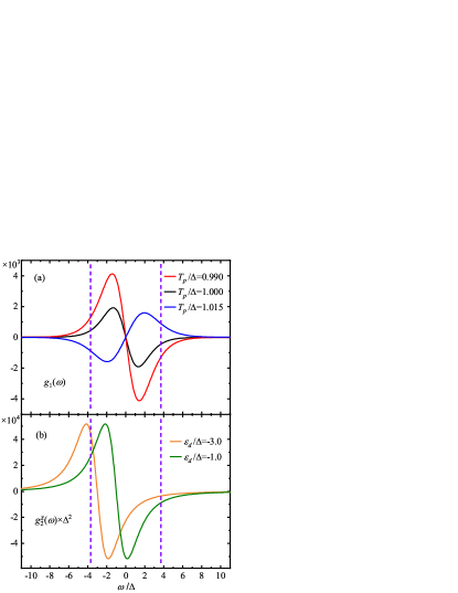
Figure 3: The lineshapes of (a) $g_{1}(\omega,T_{p})$ at various $T_{p}$ and (b) $g_{2}^{\chi}(\omega,\epsilon_{d})$ at various $\epsilon_{d}$ for a noninteracting single-impurity system. The energetic parameters of the system are the same as those adopted in Fig. 2. The region bounded by the two vertical dashed lines represents an activation energy window, $(\mu_{L}-\omega_{L},\mu_{R}+\omega_{R})$, which is determined by the Fermi distribution function for the leads: $f_{T_{\alpha},\mu_{\alpha}}(\omega)=1/[e^{(\omega-\mu_{\alpha})/T_{\alpha}}+1]$.ye2016thermodynamic Here, $\omega_{\alpha}$ is the full width at half maximum of $\frac{\partial}{\partial\omega}f_{T_{\alpha},\mu_{\alpha}}(\omega)$. Under a finite bias voltage, most of the electronic excitations are expected to occur within such an energy window.

If the ZPC is satisfied, the determined $T^{\ast,{\rm MPC}}(O)$ carries an unambiguous thermodynamic meaning, which is manifested by a correspondence relation,ye2016thermodynamic i.e., the local observable $O$ of the measured nonequilibrium system is identical to that of an equilibrium reference system with the temperature being $T^{\ast,{\rm MPC}}(O)$.

How far the system is from a quantum resonance region can be assessed by analyzing the overlap between the functions $g_{1}(\omega,T_{p})$ and $g_{2}^{\chi}(\omega,\epsilon_{d})$. For instance, Fig. 3(b) depicts the lineshapes of $g_{2}^{\chi}(\omega,\epsilon_{d})$ at various $\epsilon_{d}$ for the single-impurity system studied in Fig. 2. Apparently, when $\epsilon_{d}$ is close to zero, the function $g_{2}^{\chi}(\omega,\epsilon_{d})$ falls mainly within the activation window and thus overlaps largely with $g_{1}(\omega,T_{p})$, and the system is considered to be in-resonance. With the $\epsilon_{d}$ being shifted away from zero, the main part of $g_{2}^{\chi}(\omega,\epsilon_{d})$ gradually leaves the activation window and thus overlaps less with $g_{1}(\omega,T_{p})$, which implies that the system moves towards the off-resonance region. For the system explored in Figs. 2 and 3, the resonance and off-resonance regions are $|\epsilon_{d}|<\Delta$ and $|\epsilon_{d}|>3\Delta$, and the interstitial regions are the NR regions. A similar analysis can be carried out for a generic quantum impurity system.

Off-resonance– The impurity system is in the off-resonance region if the impurity energy level $\epsilon_{d}$ is far away from the activation window defined by $g_{1}(\omega,T_{p})$. In such a case, it is the tail of $g_{2}^{O}$ that overlaps the main body of $g_{1}$. Since $g_{2}^{O}(\omega,\epsilon_{d})$ varies rather smoothly with $\omega$ in the nonequilibrium activation window, we may use the Taylor expansion and rewrite the ZPC of Eq. (17) as

$$\delta O_{p} =\int d\omega\,g_{1}(\omega,T_{p})\,\Big{[}g_{2}^{O}(0,\epsilon_{d})+\partial_{\omega}g_{2}^{O}(0,\epsilon_{d})\,\omega$$

$$\qquad\qquad+\frac{1}{2}\,\partial_{\omega}^{2}g_{2}^{O}(\xi,\epsilon_{d})\,\omega^{2}\Big{]}$$

$$=\partial_{\omega}g_{2}^{O}(0,\epsilon_{d})\int d\omega\,g_{1}(\omega,T_{p})\,\omega$$

$$=0.$$ (18)

Here, $\partial_{\omega}\equiv\frac{\partial}{\partial\omega}$ and $\partial_{\omega}^{2}\equiv\frac{\partial^{2}}{\partial\omega^{2}}$, and $\partial_{\omega}^{2}g_{2}^{O}(\xi,\epsilon_{d})$ with $\xi\in(0,\omega)$ is the Lagrange remainder. The first equality uses the fact that $g_{1}(\omega,T_{p})$ is an odd function of $\omega$. It is thus evident that, for the single-impurity system under study, the ZPC holds universally for any local observable in the off-resonance region, i.e., $T^{\ast,{\rm MPC}}(n)=T^{\ast,{\rm MPC}}(\chi^{c})=T^{\ast,{\rm MPC}}(O)$ for any $O$.

In-resonance– In contrast, the impurity system is in the resonance region if $\epsilon_{d}$ is close to the lead chemical potential and thus lies within the nonequilibrium activation window. In this case, the value of $T^{\ast,{\rm MPC}}(O)$ may vary with the specific choice of $O$, since different local observables may respond differently to nonlocal excitations. Instead, we still see $T^{\ast,{\rm MPC}}(n)\approx T^{\ast,{\rm MPC}}(\chi^{c})$ in Fig. 2. This is because of the following relation resulting from the Taylor expansion and the first equality of Eq. (16),

$$g_{2}^{n}(\omega,\epsilon_{d}) =g_{2}^{n}(\omega,0)-\epsilon_{d}\,g_{2}^{\chi}(\omega,\xi_{1})$$

$$=g_{2}^{n}(\omega,0)-\epsilon_{d}\,g_{2}^{\chi}(\omega,\epsilon_{d})$$

$$\quad-\epsilon_{d}(\xi_{1}-\epsilon_{d})\,\partial_{\epsilon_{d}}g_{2}^{\chi}(\omega,\xi_{2}).$$ (19)

Here, $\xi_{1}\in(0,\epsilon_{d})$ and $\xi_{2}\in(\xi_{1},\epsilon_{d})$. $g_{2}^{n}(\omega,0)$ is an even function of $\omega$ and its overlap integral with $g_{1}(\omega,T_{p})$ is zero. The last term on the RHS of Eq. (19) is negligibly small since $\epsilon_{d}(\xi_{1}-\epsilon_{d})\sim\mathcal{O}(\epsilon_{d}^{2})$ and $\partial_{\epsilon_{d}}g_{2}^{\chi}(\omega,\xi_{2})$ is nearly an even function of $\omega$. Therefore, by combining Eq. (17) and Eq. (19), we find that the ZPC for $n$ is approximately equivalent to the ZPC for $\chi^{c}$, and hence $T^{\ast,{\rm MPC}}(n)\approx T^{\ast,{\rm MPC}}(\chi^{c})$.

Near-resonance– In the NR region, the product of $g_{1}(\omega,T_{p})$ and $g_{2}^{O}(\omega,\epsilon_{d})$ depends sensitively on the nature of $O$, and so is the value of $T^{\ast,{\rm MPC}}$; see Fig. 2.

From the above theoretical analysis we can conclude that the choice of local observable has little influence on $T^{\ast,{\rm MPC}}$ in the off-resonance regions. In contrast, in the resonance or NR region, the value of $T^{\ast,{\rm MPC}}$ depends on how significantly the local observable is affected by the emerging nonlocal excitations and how sensitively it varies with $T_{p}$.

When quantum resonances come into play, the $T^{\ast,{\rm MPC}}$ measured by monitoring a suitable local observable, such as the $T^{\ast,{\rm MPC}}(\chi^{c})$ depicted in Fig. 2, is still capable of identifying and quantifying the magnitude of the nonlocal excitations.

III Effect of quantum resonances on local temperatures of multi-impurity systems

III.1 Local minimal-perturbation condition

We now extend the MPC to the systems consisting of more than one impurity. For numerical convenience, a serially coupled noninteracting $N$-impurity system is considered, which is described by an AIM with

$$\hat{H}_{\rm imp} =\sum_{i=1}^{N}\epsilon_{i}\,\hat{n}_{i}+\sum_{i=1}^{N-1}\big{[}t\,(\hat{a}_{i\uparrow}^{{\dagger}}\hat{a}_{{i+1}\uparrow}+\hat{a}_{i\downarrow}^{{\dagger}}\hat{a}_{{i+1}\downarrow})+{\rm H.c.}\big{]},$$ (20)

where $\epsilon_{i}$ is the on-site energy of the $i$th impurity, and $t$ is the coupling strength between two adjacent impurities. As illustrated in Fig. 4(a), the $N$-impurity system forms a linear chain, in which the left (right) lead is coupled only to the first ($N$th) impurity with the coupling strength being $\Delta_{L}$ ($\Delta_{R}$).

In principle the MPC of Eq. (5) can be formally extended to determine the local temperature and local chemical potential of each individual impurity as follows,

$$\left\{\begin{aligned} &{I_{p,i}(T^{\ast}_{i},\mu^{\ast}_{i})=0},\\ &(T^{\ast}_{i},\mu^{\ast}_{i})={\arg\min_{(T_{p},\mu_{p})}|\delta O_{p,i}(T_{p},\mu_{p})|}\end{aligned}\right..$$ (21)

Here, the probe is weakly coupled to the $i$th impurity. As a natural extension of the MPC, Eq. (21) is referred to as the local MPC (LMPC). However, in practice the extension from MPC to LMPC is not always straightforward. This is because it is often difficult to acquire the minimally perturbed value of a particular local observable $O_{{\rm ref},i}$. To circumvent this problem, we can choose a local observable whose reference value is known by the intrinsic symmetry of the system.

For instance, if the investigated multi-impurity system is spin unpolarized, i.e, all the energetic parameters in Eq. (20) are spin independent, by coupling a probe to an impurity, the electric current through the probe should also be spin unpolarized. In other words, if the local observable $O$ is chosen to be the magnetic susceptibility of the electric current through the coupled probe, $\chi^{I}_{p,i}\equiv\frac{\partial I_{pz,i}}{\partial H_{z}}|_{H_{z}\rightarrow 0}$ with $I_{pz,i}=\frac{1}{2}(I_{p,i\uparrow}-I_{p,i\downarrow})$, its minimally perturbed value is just $\chi^{I}_{{\rm ref},i}=0$, if the $i$th impurity is spin unpolarized in the presence of the probe. Note that for the measurement of $(T^{\ast}_{i},\mu^{\ast}_{i})$ the magnetic field $H_{z}$ is applied exclusively on the $i$th impurity. In contrast, it is much harder to determine the value of $\chi^{m}_{{\rm ref},i}$ directly for the $i$th impurity.

For a single-impurity system, the thermodynamic meaning of $T^{\ast,{\rm MPC}}$ has been elucidated via a correspondence condition between the nonequilibrium system under study and a reference system in thermal equilibrium, i.e., $O_{\rm neq}=O_{\rm eq}$, provided that the $T^{\ast,{\rm MPC}}(O)$ and $\mu^{\ast,{\rm MPC}}(O)$ of the nonequilibrium system coincide with the equilibrium temperature and chemical potential of the reference system.ye2016thermodynamic

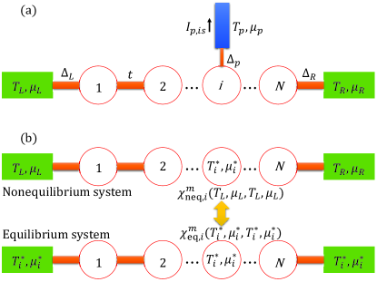
Figure 4: (a) Schematic illustration of a serially coupled $N$-impurity system. The first ($N$th) impurity is coupled to the left (right) lead. The probe is weakly coupled to the $i$th impurity under study, and the spin-specific electric current flowing into the probe $I_{p,is}$ is monitored. (b) Schematic illustration of the correspondence relation which states that the local magnetic susceptibility of the $i$th impurity in a nonequilibrium system is equal to that in an equilibrium system, provided that they have the same local temperature and local chemical potential.

In the following, we demonstrate that a correspondence relation can also be established for a multi-impurity system with the $\chi^{I}_{p,i}$ chosen as the local observable.

To facilitate the theoretical analysis, we consider a serially coupled noninteracting double-impurity system. By applying a local magnetic field $H_{z}$ to the $i$th impurity, the impurity level is subject to a Zeeman splitting which is assumed to be linearly proportional to $H_{z}$. Consequently, for the spin-unpolarized system under study, we have $\chi^{I}_{p,i}=\mathcal{C}\frac{\partial I_{p,i\uparrow}}{\partial\epsilon_{i}}$ with $\mathcal{C}$ being a constant. Without loss of generality, the probe is coupled to the first impurity. In the wide-band limit, the probe-induced perturbation to $\chi^{I}_{p,1}$ is expressed as

$$\delta\chi^{I}_{p,1} =-\mathcal{C}\,\frac{i}{\pi}\int d\omega\,\Gamma_{p}(\omega)\,\partial_{\epsilon_{1}}\Big{\{}G^{<}_{\uparrow,11}(\omega)$$

$$\qquad\qquad+2if_{T_{p},\mu_{p}}(\omega)\,{\rm Im}[G^{r}_{\uparrow,11}(\omega)]\Big{\}}$$

$$=\mathcal{C}\,\frac{2\Delta_{p}}{\pi}\int d\omega\ \Big{\{}\Delta_{L}\left[(\omega-\epsilon_{2})^{2}+\Delta_{R}^{2}\right]$$

$$\quad\times[f_{T_{L},\mu_{L}}(\omega)-f_{T_{p},\mu_{p}}(\omega)]+t^{2}\Delta_{R}$$

$$\quad\times[f_{T_{R},\mu_{R}}(\omega)-f_{T_{p},\mu_{p}}(\omega)]\Big{\}}\,\partial_{\epsilon_{1}}|B_{p1}(\omega)|^{2},$$ (22)

where

$$B_{p1}(\omega)=\frac{1}{[\omega-\epsilon_{1}+i(\Delta_{L}+\Delta_{p})](\omega-\epsilon_{2}+i\Delta_{R})-t^{2}}.$$ (23)

Similarly, for a spin-unpolarized system, the local magnetic susceptibility of the $i$th impurity can be rewritten as $\chi^{m}_{i}=\mathcal{C}^{\prime}\frac{\partial n_{i\uparrow}}{\partial\epsilon_{i}}$, with $\mathcal{C}^{\prime}$ being a constant different from $\mathcal{C}$. In the nonequilibrium steady state characterized by the temperatures and chemical potentials of the left and right leads, $(T_{L},\mu_{L},T_{R},\mu_{R})$, the value of $\chi^{m}_{1}$ in the absence of the probe is

$$\chi^{m}_{{\rm neq},1} =\mathcal{C^{\prime}}\frac{1}{2\pi i}\int d\omega\,\,\partial_{\epsilon_{1}}[G^{<}_{\uparrow,11}(\omega)]$$

$$=\mathcal{C^{\prime}}\,\frac{1}{\pi}\int d\omega\,\Big{\{}\Delta_{L}\left[(\omega-\epsilon_{2})^{2}+\Delta_{R}^{2}\right]f_{T_{L},\mu_{L}}(\omega)$$

$$\qquad\qquad+t^{2}\Delta_{R}f_{T_{R},\mu_{R}}(\omega)\Big{\}}\,\partial_{\epsilon_{1}}|B(\omega)|^{2},$$ (24)

where $B(\omega)=B_{p1}(\omega)|_{\Delta_{p}=0}$. For the reference system in a thermal equilibrium state characterized by the background temperature $T^{\ast}_{1}$ and chemical potential $\mu^{\ast}_{1}$, the corresponding $\chi^{m}_{1}$ is expressed in a form similar to Eq. (24), but with $(T_{L},\mu_{L},T_{R},\mu_{R})$ replaced by $(T^{\ast}_{1},\mu^{\ast}_{1},T^{\ast}_{1},\mu^{\ast}_{1})$. Therefore, the difference between $\chi^{m}_{{\rm neq},1}$ and $\chi^{m}_{{\rm eq},1}$ is

$$\chi^{m}_{{\rm neq},1}(T_{L},\mu_{L},T_{R},\mu_{R})-\chi^{m}_{{\rm eq},1}(T^{\ast}_{1},\mu^{\ast}_{1},T^{\ast}_{1},\mu^{\ast}_{1})$$

$$= \frac{\mathcal{C^{\prime}}}{\pi}\int d\omega\ \Big{\{}\Delta_{L}\left[(\omega-\epsilon_{2})^{2}+\Delta_{R}^{2}\right]\left[f_{T_{L},\mu_{L}}(\omega)-f_{T^{\ast}_{1},\mu^{\ast}_{1}}(\omega)\right]$$

$$\quad+t^{2}\Delta_{R}\left[f_{T_{R},\mu_{R}}(\omega)-f_{T^{\ast}_{1},\mu^{\ast}_{1}}(\omega)\right]\Big{\}}\,\partial_{\epsilon_{1}}|B(\omega)|^{2}.$$ (25)

By comparing Eq. (III.1) and Eq. (25), it is easy to recognize that the relation

$$\chi^{m}_{{\rm neq},1}(T_{L},\mu_{L},T_{R},\mu_{R})=\chi^{m}_{{\rm eq},1}(T_{1}^{\ast},\mu_{1}^{\ast},T_{1}^{\ast},\mu_{1}^{\ast})$$ (26)

holds provided that

$$\left.\frac{\delta\chi^{I}_{p,1}(T_{1}^{\ast},\mu_{1}^{\ast})}{\Delta_{p}}\right|_{\Delta_{p}\to 0}=0.$$ (27)

A similar relation can be established for the second impurity of the double-impurity system, or any impurity of a generic multi-impurity system; see Fig. 4(b).

Equation (27) is the local ZPC for the local observable $\chi^{I}_{p,1}$, and the thermodynamic meaning of the resulting ($T^{\ast}_{1},\mu^{\ast}_{1}$) is unambiguously given by Eq. (26). When the local ZPC of Eq. (27) cannot be reached, such as in the NR region, the LMPC of Eq. (21) with $O_{i}=\chi^{I}_{p,i}$ still yields a unique $T^{\ast}_{i}$ which could characterize the emergence of quantum resonance effects; see Sec. III.2 and Sec. III.3 for details.

III.2 Validity of LMPC for single impurity systems

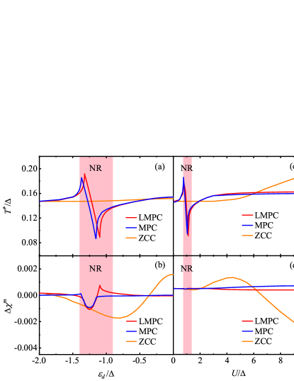
Figure 5: (a) $T^{\ast}$ determined by the ZCC, MPC (with $O=\chi^{m}$), and LMPC (with $O=\chi^{I}_{p}$) as functions of $\epsilon_{d}$ for a noninteracting single-impurity system under an antisymmetric bias voltage of $\mu_{R}=-\mu_{L}=V/2=0.2\Delta$. (b) The relative deviation from the correspondence relation, $\Delta\chi^{m}=\chi^{m}_{\rm eq}/\chi^{m}_{\rm neq}-1$, versus $\epsilon_{d}$. (c) $T^{\ast}$ determined by the ZCC, MPC, and LMPC as functions of $U$ for an interacting single-impurity system with $\epsilon_{d}=-2\Delta$ under the same antisymmetric bias voltage. (d) The relative deviation $\Delta\chi^{m}$ versus $U$. Other energetic parameters adopted are (in units of $\Delta$): $T_{L}=T_{R}=0.1$, $\Delta_{L}=\Delta_{R}=0.5$, and $W_{L}=W_{R}=20$. The shaded areas represent the NR regions.

Before applying the LMPC-based protocol to multi-impurity systems, we first examine its consistency with the MPC-based protocol for single-impurity systems. In principle, the LMPC-based protocol with $\chi^{I}_{p}$ as the local observable is equivalent to the MPC-based definition with $O=\chi^{m}$. This is because they both lead to the correspondence relation $\chi^{m}_{{\rm neq}}(T_{L},\mu_{L},T_{R},\mu_{R})=\chi^{m}_{{\rm eq}}(T^{\ast},\mu^{\ast},T^{\ast},\mu^{\ast})$, provided that the ZPC for the local observable can be achieved. Nevertheless, for a real system the equality in the above relation is subject to a small error due to the finite band width of the leads, which could affect the two local observables somewhat differently. Consequently, in Fig. 5 the resulting $T^{\ast,{\rm MPC}}$ and $T^{\ast,{\rm LMPC}}$ exhibit some minor deviation.

Figure 5(a) shows the $T^{\ast}$ of a noninteracting single-impurity system under an antisymmetric bias voltage as a function of $\epsilon_{d}$. It is found that, while the $T^{\ast,{\rm LMPC}}$ agree closely with the $T^{\ast,{\rm MPC}}$ outside the NR region, they display an appreciable difference in the NR region despite the overall similar lineshape.

In the NR region, if the value of the monitored local observable (such as $\chi^{I}_{p}$ and $\chi^{m}$) is strongly affected by the emergence of quantum resonances, it could be difficult to reach the ZPC by simply tuning the $T_{p}$. In such a case, $T^{\ast}$ has to be determined by searching for the $T_{p}$ that yields a minimal nonzero perturbation to $O$ ($\delta O_{p}$). Thus, the resulting $T^{\ast,{\rm LMPC}}$ or $T^{\ast,{\rm MPC}}$ may exhibit large oscillations and deviate from each other because the minimal $\delta O_{p}$ tends to vary sensitively with the nonlocal excitations introduced by the emerging quantum resonance.

Figure 5(b) depicts the relative deviation of $\chi^{m}$ of the nonequilibrium impurity system from that of the reference equilibrium system, $\Delta\chi^{m}=\chi^{m}_{\rm eq}/\chi^{m}_{\rm neq}-1$. Evidently, while $\Delta\chi^{m}$ almost vanishes with either $T^{\ast,{\rm MPC}}$ or $T^{\ast,{\rm LMPC}}$, it remains of a finite magnitude in the NR region where the ZPC cannot be reached. In contrast, the $T^{\ast,{\rm ZCC}}$ are almost constant in the whole range of $\epsilon_{d}$ with a considerably larger $\Delta\chi^{m}$, and they show no sign of quantum resonances at all.

Figures 5(c) and 5(d) depict the $T^{\ast}$ and $\Delta\chi^{m}$ of an interacting single-impurity system under an antisymmetric bias voltage as a function of $U$, respectively. Similar to the case of a noninteracting impurity, as long as the ZPC can be satisfied, the $T^{\ast,{\rm LMPC}}$ and $T^{\ast,{\rm MPC}}$ agree closely with each other, otherwise they display a minor difference. It is worth pointing out that the low background temperature enables the formation of Kondo states,Yigal1993Low which provide resonant channels for electrons to transport across the impurity. Therefore, the system remains in the resonance region with a sufficiently large $U$ ($U>-\epsilon_{d}$). Again, the $T^{\ast,{\rm ZCC}}$ vary rather smoothly and do not reflect the formation of quantum resonant states at all.

The above results clearly verify that the newly proposed LMPC is generally consistent with the original MPC for single-impurity systems.

III.3 Local temperatures of multi-impurity systems and the effect of quantum resonances

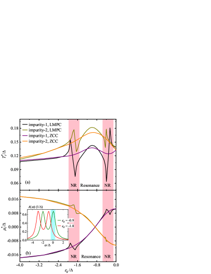
Figure 6: Evolution of (a) $T^{\ast}_{i}$ and (b) $\mu^{\ast}_{i}$ determined by the ZCC and the LMPC with the variation of $\epsilon_{i}=\epsilon_{d}$ for a noninteracting double-impurity system under an antisymmetric bias voltage of $\mu_{R}=-\mu_{L}=V/2=0.2\Delta$. Other energetic parameters adopted are (in units of $\Delta$): $T_{L}=T_{R}=0.1$, $U=0$, $t=1$, $\Delta_{L}=\Delta_{R}=0.5$, and $W_{L}=W_{R}=20$. The shaded areas in the main panels represent the NR regions. The inset of (b) depicts the total spectral function of the two impurities $A(\omega)$ at different $\epsilon_{d}$, where the shaded area indicates the nonequilibrium activation window.

We now employ the LMPC-based protocol to investigate the distribution of local temperatures in a double-impurity system under an antisymmetric bias voltage. Here, the two impurities are presumed to have the same onsite energy, i.e., $\epsilon_{i}=\epsilon_{d}$.

Figure 6 depicts the evolution of $(T^{\ast}_{i},\mu^{\ast}_{i})$ of the two impurities with the variation of $\epsilon_{d}$. In analogy with the case of single-impurity systems, while the $T_{i}^{\ast,{\rm LMPC}}$ agree well with the $T^{\ast,{\rm ZCC}}_{i}$ in the absence of resonance, they are distinctly different in the two NR regions.

It is worth noting that $T^{\ast}_{1}<T^{\ast}_{2}$ at almost any $\epsilon_{d}<0$, which can be explained as follows. With $\epsilon_{d}<0$ the total spectral function, $A(\omega)$, of the two impurities has a distribution more on the negative energy side, and this means that the double-impurity system has a positive Seebeck coefficient $S$.Don0211747 ; Ye2014Thermopower Consequently, the voltage-generated heat current between the two impurities follows the opposite direction of the electric current, i.e., from left to right. Such a heat current thus creates an internal thermal gradient across the two impurities with $T^{\ast}_{1}<T^{\ast}_{2}$.

At $\epsilon_{d}=0$, $A(\omega)$ becomes an even function of $\omega$. As a result we have $S=0$, and hence the voltage-generated internal thermal gradient also becomes zero, i.e., $T^{\ast}_{1}=T^{\ast}_{2}$. This is indeed confirmed by our calculation results shown in Fig. 6(a). Furthermore, it is also inferred that $T^{\ast}_{1}>T^{\ast}_{2}$ at $\epsilon_{d}>0$ (data not shown).

It is also interesting to observe that, while the left (right) lead has a lower (higher) chemical potential, the $\mu^{\ast}_{i}$ of the neighboring impurity is not necessarily lower (higher); see Fig. 6(b). The fluctuation of $\mu^{\ast}_{i}$ manifests the quantum coherence nature of the electron transport driven by the bias voltage. In particular, $\mu^{\ast}_{1}=\mu^{\ast}_{2}=0$ at $\epsilon_{d}=-0.9\Delta$, where a resonant state resides right at the center of the nonequilibrium activation window; see the $A(\omega)$ in the inset of Fig. 6(b). The uniformity of $\mu^{\ast}_{i}$ indicates that the voltage-driven excitations are predominantly nonlocal as they occur via the resonant state which involves both impurities.

In Fig. 6, it is again apparent that the $(T^{\ast}_{i},\mu^{\ast}_{i})$ predicted by the ZCC vary smoothly with $\epsilon_{d}$, and completely neglect the existence of nonlocal excitations; whereas those determined by the LMPC exhibit large oscillations in the NR regions, which clearly accentuates the emergence of a quantum resonance.

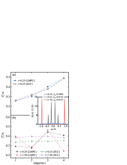
Figure 7: Local temperature profile $T^{\ast}_{i}$ determined by the ZCC and the LMPC for a noninteracting four-impurity chain under a thermal bias with (a) a strong impurity-lead coupling of $\Delta_{\alpha}=0.5\Delta$ ($\alpha=L,R$) and (b) a weak impurity-lead coupling of $\Delta_{\alpha}=0.0125\Delta$. Other energetic parameters adopted are (in units of $\Delta$): $\epsilon_{i}=\epsilon_{d}=0$, $U=0$, $\mu_{L}=\mu_{R}=0$, $T_{L}=0.25$, $T_{R}=0.5$, and $W_{L}=W_{R}=5$. The inset depicts the system spectral function $A(\omega)$ at different $t$ and $\Delta_{\alpha}$.

We proceed to study a linear chain comprised of four noninteracting impurities subject to a thermal bias, i.e., $T_{L}<T_{R}$. The local chemical potential on each impurity $\mu^{\ast}_{i}$ is nearly zero due to the absence of bias voltage. Figure 7 depicts the distribution of $T^{\ast}_{i}$ along the chain determined by the ZCC and the LMPC for various values of $t$ and $\Delta_{\alpha}$ ($\alpha=L,R$).

As shown in Fig. 7(a), when the terminal impurities are coupled strongly to the leads, both the ZCC and the LMPC predict the $T^{\ast}_{i}$ vary almost linearly with $i$, i.e., the distribution of local temperature along the chain obeys the classical Fourier’s law.Zhang2019local Note that here the restoration of the Fourier’s law is not because of disorderDub09115415 or dephasing caused by an external source,Dub09042101 which are absent from the AIM under study. Instead, the linear profile of $T^{\ast}_{i}$ is associated with the substantial broadening of the spectral peaks in $A(\omega)$.Inu184304 This means that the thermal transport process involves electronic states in a wide range of energies. The phases of these states are averaged out when $T^{\ast}_{i}$ are measured, which leads to a classical-like behavior. As the inset of Fig. 7 shows, the impurity-lead coupling $\Delta_{\alpha}$ ($\alpha=L$ or $R$) affects significantly the sharpness of the peaks, while the coupling strength $t$ between two adjacent impurities has important influence on the distance of neighboring peaks in a system.

In contrast, Fig. 7(b) concerns another scenario in which the impurity-lead coupling is extremely weak, so that the thermal transport occurs almost exclusively via the quantum resonant states formed on the chain. In such a scenario, the ZCC and the LMPC yield very different predictions on the distribution of $T^{\ast}_{i}$. Specifically, the $T^{\ast,{\rm ZCC}}_{i}$ of all four impurities is close to a certain value between $T_{L}$ and $T_{R}$, while the $T_{i}^{\ast,{\rm LMPC}}$ exhibit large oscillations along the chain, which clearly violates the Fourier’s law.

Inui et al. Inu184304 have reported strong oscillations of temperature distribution in a graphene flake weakly coupled to the electrodes under a thermal bias due to quantum interference. But in their study the local temperatures $T^{\ast,{\rm ZCC}}_{i}$ still remain constant on a relatively small scale in the weak-coupling regime, similar to the curve of $T^{\ast,{\rm ZCC}}_{i}$ in Fig. 7(b). Note that the chain in our work is very short, so that even with weak impurity-lead couplings the ZCC-defined $T^{\ast}_{i}$ cannot reveal prominent oscillations. In contrast, the LMPC-defined $T^{\ast,{\rm LMCP}}_{i}$ oscillations in our work are much more significant. In the strong-coupling regime, the temperature profile for the graphene flake is much closer to that predicted by classical Fourier’s law,Inu184304 which is consistent with our results in Fig. 7(a).

IV Concluding remarks

In conclusion, our study has demonstrated that, while the MPC could yield a unique local temperature for a given local observable $\hat{O}$, the value of $T^{\ast,{\rm MPC}}$ may vary with the specific choice of $\hat{O}$, particularly in the NR region where both the local and nonlocal excitations could take place inside a quantum impurity system. It is also noticed that, while $T^{\ast,{\rm MPC}}$ agrees quantitatively to $T^{\ast,{\rm ZCC}}$ away from the in-resonance region, their difference is appreciable in the NR region. This indicates that, when quantum resonant states emerge in the system, it is difficult to fully eliminate the influence of the probe on the local observable $O$ by tuning $T_{p}$ and $\mu_{p}$, because of the presence of nonlocal excitations.

We have also proposed an operational protocol based on the LMPC, which extends the operational principle of MPC to multi-impurity systems. Using the LMPC, we studied the effect of quantum resonances on the local temperatures of noninteracting multi-impurity systems. We found that the $T^{\ast,{\rm LMPC}}_{i}$ of double-impurity systems under an antisymmetric bias voltage agree well with the $T^{\ast,{\rm ZCC}}_{i}$ in the absence of resonances. On the other hand, they are distinctly different in the two NR regions, which is analogous to the case of single-impurity systems. Applying the LMPC to a linear chain of four impurities, we found that the strong quantum resonance effects lead to prominent oscillations in the local temperature, which are not observed with the ZCC-based definition.

It is important to point out that the practical implementation of the MPC- and LMPC-based protocols is very straightforward, as they do not require the direct measurement of heat currents. Moreover, in the existing experimental and theoretical works, the measured local temperature is often associated with concrete physical properties, such as thermoelectricity,mills1998scanning ; luo1996nanofabrication electrical resistance,zhang2011batch ; pylkki1994scanning thermal expansion,nakabeppu1995scanning fluorescence,saidi2009scanning energy reactance,ludovico2014dynamical ; ludovico2018probing etc. In the present work, the local temperature determined by the MPC- or LMPC-based protocol is closely related to the monitored local observable. The measured local temperature can be unambiguously interpreted by the correspondence relation, i.e., the monitored local observable of the nonequilibrium system under study is identical to that of an equilibrium reference system, provided that the perturbation induced by the probe can be completely suppressed by tuning $T_{p}$ and $\mu_{p}$.

Appendix A MPC zero perturbation implies zero energy and particle flows: A formal proof

Consider a system interacting with several environments $\alpha$. The total Hamiltonian is $\hat{H}_{{}_{\rm T}}=\hat{H}_{{}_{\rm S}}+\sum_{\alpha}(\hat{H}_{\alpha}+\hat{H}_{{\rm s}\alpha})$, where $\hat{H}_{{}_{\rm S}}$ represents the primary system of interest, $\hat{H}_{\alpha}$ represents the $\alpha$th environment ($\alpha=p$ labels the probe), and $\hat{H}_{{\rm s}\alpha}$ is the system-environment interaction. The density matrix of the total system $\rho_{{}_{\rm T}}$ satisfies the equation

$$\dot{\rho}_{{}_{\rm T}}=-i[\hat{H}_{{}_{\rm T}},\rho_{{}_{\rm T}}].$$ (28)

We define $\rho\equiv{\rm tr}_{{}_{\rm B}}(\rho_{{}_{\rm T}})$ as the reduced density matrix of the primary system, with ${\rm tr}_{{}_{\rm B}}$ denoting a trace over all the environment degrees of freedom. A quantum master equation (QME) for $\rho$ can be formally written as

$$\dot{\rho}=-i[\hat{H}_{{}_{\rm S}},\rho]+\sum_{\alpha}\mathcal{R}_{\alpha}[\rho],$$ (29)

where $\mathcal{R}_{\alpha}[\rho]$ represents the dissipation term between the system and the $\alpha$th environment.

In the following, we give a formal proof showing that $\mathcal{R}_{\alpha}[\rho]=0$ implies $I_{\alpha}=0$ and $J^{E}_{\alpha}=0$ for the $\alpha$th reservoir environment coupled to an open system at a stationary state, where $I_{\alpha}$ and $J^{E}_{\alpha}$ are the electrical and energy currents between the system and the $\alpha$th reservoir, respectively.

By referring to Eq. (28), the dissipation term $\mathcal{R}_{\alpha}[\rho]$ in Eq. (29) originates from the following expression

$$\mathcal{R}_{\alpha}[\rho]=-i\,{\rm tr}_{{}_{\rm B}}\{[\hat{H}_{{\rm s}\alpha}+\hat{H}_{\alpha},\rho_{{}_{\rm T}}]\}.$$ (30)

Consider first the electric current between the system and the $\alpha$th reservoir, which is defined by

$$I_{\alpha}\equiv\dot{N}_{\alpha}(t)={\rm tr}_{{}_{\rm T}}\{\hat{N}_{\alpha}\dot{\rho}_{{}_{\rm T}}\}=-i\,\langle[\hat{N}_{\alpha},H_{{\rm s}\alpha}]\rangle.$$ (31)

Here, $\langle\cdots\rangle\equiv{\rm tr}_{{}_{\rm T}}\{\cdots\rho_{{}_{\rm T}}\}$, and we have used the fact that the number of particles operator $\hat{N}_{\alpha}$ commutes with $\hat{H}_{{}_{\rm S}}$ and $\hat{H}_{\alpha^{\prime}}$. On the other hand, the QME for $\rho$ gives rise to a formula for the conservation of particles, $\dot{N}_{{}_{\rm S}}(t)={\rm tr}_{{}_{\rm S}}\{\hat{N}_{{}_{\rm S}}\dot{\rho}\}=-\sum_{\alpha}\tilde{I}_{\alpha}$, where

$$\tilde{I}_{\alpha}\equiv-{\rm tr}_{{}_{\rm S}}\{\hat{N}_{{}_{\rm S}}\mathcal{R}_{\alpha}[\rho]\}=i\,\langle[\hat{N}_{{}_{\rm S}},H_{{\rm s}\alpha}]\rangle.$$ (32)

The last equality of Eq. (32) uses the fact that $\hat{N}_{{}_{\rm S}}$ commutes with $\hat{H}_{\alpha}$. By comparing Eq. (31) and Eq. (32), we have

$$I_{\alpha}=\tilde{I}_{\alpha}-i\,\langle[\hat{N}_{\alpha}+\hat{N}_{{}_{\rm S}},H_{{\rm s}\alpha}]\rangle.$$ (33)

If every term in the interaction Hamiltonian $\hat{H}_{{\rm s}\alpha}$ conserves the number of particles within the system and the $\alpha$th environment (e.g., in the Anderson impurity model $\hat{H}_{{\rm s}\alpha}$ causes electron transfer only between the impurity and the $\alpha$th reservoir), we have $[\hat{N}_{\alpha}+\hat{N}_{{}_{\rm S}},\hat{H}_{{\rm s}\alpha}]=0$. Thus, $\mathcal{R}_{\alpha}[\rho]=0$ immediately leads to $I_{\alpha}=\tilde{I}_{\alpha}=0$.

Consider then the energy flow between the system and the $\alpha$th environment, which is defined by

$$J^{E}_{\alpha}\equiv\dot{E}_{\alpha}(t)=-i\,\langle[\hat{H}_{\alpha},\hat{H}_{{\rm s}\alpha}]\rangle.$$ (34)

Similarly, the QME for $\rho$ gives rise to a formula for the conservation of energy, $\dot{E}_{{}_{\rm S}}(t)={\rm tr}_{{}_{\rm S}}\{\hat{H}_{{}_{\rm S}}\dot{\rho}\}=-\sum_{\alpha}\tilde{J}^{E}_{\alpha}$, where

$$\tilde{J}^{E}_{\alpha}\equiv-{\rm tr}_{{}_{\rm S}}\{\hat{H}_{{}_{\rm S}}\mathcal{R}_{\alpha}[\rho]\}=i\,\langle[\hat{H}_{{}_{\rm S}},\hat{H}_{{\rm s}\alpha}]\rangle.$$ (35)

Here, we have used the fact that $\hat{H}_{{}_{\rm S}}$ commutes with $\hat{H}_{\alpha}$. By comparing Eq. (34) with Eq. (35), we have

$$J^{E}_{\alpha} =\tilde{J}^{E}_{\alpha}-i\,\langle[\hat{H}_{{}_{\rm T}},\hat{H}_{{\rm s}\alpha}]\rangle-i\sum_{\alpha^{\prime}\neq\alpha}{\rm tr}_{{}_{\rm T}}\{[\hat{H}_{{\rm s}\alpha},\hat{H}_{{\rm s}\alpha^{\prime}}]\,\rho_{{}_{\rm T}}\}$$

$$=-{\rm tr}_{{}_{\rm S}}\{\hat{H}_{{}_{\rm S}}\mathcal{R}_{\alpha}[\rho]\}-{\rm tr}_{{}_{\rm T}}\{\hat{H}_{{\rm s}\alpha}\dot{\rho}_{{}_{\rm T}}\}-i\sum_{\alpha^{\prime}\neq\alpha}\langle[\hat{H}_{{\rm s}\alpha},H_{{\rm s}\alpha^{\prime}}]\rangle.$$ (36)

Note that $\sum_{\alpha}\sum_{\alpha^{\prime}\neq\alpha}[\hat{H}_{{\rm s}\alpha},\hat{H}_{{\rm s}\alpha^{\prime}}]=0$.

Clearly, $\mathcal{R}_{\alpha}[\rho]=0$ alone does not guarantee $J^{E}_{\alpha}=0$. Further consideration is needed for the two other terms on the right-hand side of Eq. (A). First, we have $[\hat{H}_{{\rm s}\alpha},\hat{H}_{{\rm s}\alpha^{\prime}}]=0$ if $\hat{H}_{{\rm s}\alpha}$ and $\hat{H}_{{\rm s}\alpha^{\prime}}$ involve the system’s different degrees of freedom; otherwise, $\langle\hat{H}_{{\rm s}\alpha}\hat{H}_{{\rm s}\alpha^{\prime}}\rangle$ represents the covariance between a stochastic variable of the $\alpha$th environment and a stochastic variable of the $\alpha^{\prime}$th environment. Such a covariance is usually zero because the two environments are statistically independent. Moreover, the term ${\rm tr}_{{}_{\rm T}}\{\hat{H}_{{\rm s}\alpha}\dot{\rho}_{{}_{\rm T}}\}$ can be interpreted as the rate at which the interaction energy between the system and the $\alpha$th environment [$E_{{\rm s}\alpha}(t)$] varies with time. Such a rate is zero when the total system reaches a stationary state, (cf. Fig. 1 of Ref. Son17064308, ). We thus conclude that $\mathcal{R}_{\alpha}[\rho]=0$ leads to $J^{E}_{\alpha}=0$ for the system at a stationary state.

Finally, the heat current between the system and the $\alpha$th reservoir is also zero, i.e., $J^{H}_{\alpha}=J^{E}_{\alpha}-\mu_{\alpha}I_{\alpha}=0$.

References

- (1) D. Zhang, X. Zheng, and M. Di Ventra, Phys. Rep. 830, 1 (2019).
- (2) E. A. Hoffmann, H. A. Nilsson, J. E. Matthews, N. Nakpathomkun, A. I. Persson, L. Samuelson, and H. Linke, Nano Lett. 9, 779 (2009).
- (3) F. Menges, H. Riel, A. Stemmer, C. Dimitrakopoulos, and B. Gotsmann, Phys. Rev. Lett. 111, 205901 (2013).
- (4) F. Menges, P. Mensch, H. Schmid, H. Riel, A. Stemmer, and B. Gotsmann, Nat. Commun. 7, 10874 (2016).
- (5) S. Inui, C. A. Stafford, and J. P. Bergfield, ACS Nano 12, 4304 (2018).
- (6) W. Lee, K. Kim, W. Jeong, L. A. Zotti, F. Pauly, J. C. Cuevas, and P. Reddy, Nature (London) 498, 209 (2013).
- (7) L. Cui, R. Miao, K. Wang, D. Thompson, L. A. Zotti, J. C. Cuevas, E. Meyhofer, and P. Reddy, Nat. Nanotechnol. 13, 122 (2018).
- (8) D. Novko, J. C. Tremblay, M. Alducin, and J. I. Juaristi, Phys. Rev. Lett. 122, 016806 (2019).
- (9) M. P. Zeidler, C. Tan, Y. Bellaiche, S. Cherry, S. Häder, U. Gayko, and N. Perrimon, Nat. Biotechnol. 22, 871 (2004).
- (10) G. Kucsko, P. C. Maurer, N. Y. Yao, M. Kubo, H. J. Noh, P. K. Lo, H. Park, and M. D. Lukin, Nature (London) 500, 54 (2013).
- (11) Y.-M. He and B.-G. Ma, Sci. Rep. 6, 26737 (2016).
- (12) S. Sadat, E. Meyhofer, and P. Reddy, Rev. Sci. Instrum. 83, 084902 (2012).
- (13) M. Mecklenburg, W. A. Hubbard, E. R. White, R. Dhall, S. B. Cronin, S. Aloni, and B. C. Regan, Science 347, 629 (2015).
- (14) K. L. Grosse, M.-H. Bae, F. Lian, E. Pop, and W. P. King, Nat. Nanotechnol. 6, 287 (2011).
- (15) S. P. Gurrum, Y. K. Joshi, W. P. King, and K. Ramakrishna, J. Heat Transfer. 127, 809 (2005).
- (16) M. Di Ventra, Electrical Transport in Nanoscale Systems, Cambridge University Press, Cambridge, 2008.
- (17) S. Liu, A. Nurbawono, and C. Zhang, Sci. Rep. 5, 15386 (2015).
- (18) Z. Huang, B. Xu, Y. Chen, M. Di Ventra, and N. Tao, Nano Lett. 6, 1240 (2006).
- (19) Z. Huang, F. Chen, R. D’agosta, P. A. Bennett, M. Di Ventra, and N. Tao, Nat. Nanotechnol. 2, 698 (2007).
- (20) K. Kim, W. Jeong, W. Lee, S. Sadat, D. Thompson, E. Meyhofer, and P. Reddy, Appl. Phys. Lett. 105, 203107 (2014).
- (21) H. Thierschmann, R. Sánchez, B. Sothmann, F. Arnold, C. Heyn, W. Hansen, H. Buhmann, and L. W. Molenkamp, Nat. Nanotechnol. 10, 854 (2015).
- (22) I. Lončarić, M. Alducin, P. Saalfrank, and J. I. Juaristi, Phys. Rev. B 93, 014301 (2016).
- (23) J. C. Idrobo, A. R. Lupini, T. Feng, R. R. Unocic, F. S. Walden, D. S. Gardiner, T. C. Lovejoy, N. Dellby, S. T. Pantelides, and O. L. Krivanek, Phys. Rev. Lett. 120, 095901 (2018).
- (24) H. E. D. Scovil and E. O. Schulz-DuBois, Phys. Rev. Lett. 2, 262 (1959).
- (25) F. L. Curzon and B. Ahlborn, Am. J. Phys. 43, 22 (1975).
- (26) E. H. Lieb and J. Yngvason, Phys. Rep. 310, 1 (1999).
- (27) A. E. Allahverdyan and T. M. Nieuwenhuizen, Phys. Rev. E 64, 056117 (2001).
- (28) J. Casas-Vázquez and D. Jou, Rep. Prog. Phys. 66, 1937 (2003).
- (29) T. D. Kieu, Phys. Rev. Lett. 93, 140403 (2004).
- (30) C. Bustamante, J. Liphardt, and F. Ritort, Phys. Today 58, 43 (2005).
- (31) C. Hörhammer and H. Büttner, J. Stat. Phys. 133, 1161 (2008).
- (32) J. P. Bergfield and C. A. Stafford, Phys. Rev. B 79, 245125 (2009).
- (33) A. Levy, R. Alicki, and R. Kosloff, Phys. Rev. E 85, 061126 (2012).
- (34) M. Horodecki and J. Oppenheim, Nat. Commun. 4, 2059 (2013).
- (35) P. Skrzypczyk, A. J. Short, and S. Popescu, Nat. Commun. 5, 4185 (2014).
- (36) A. Ü. C. Hardal and Ö. E. Müstecaplıoğlu, Sci. Rep. 5, 12953 (2015).
- (37) G. Clos, D. Porras, U. Warring, and T. Schaetz, Phys. Rev. Lett. 117, 170401 (2016).
- (38) A. Puglisi, A. Sarracino, and A. Vulpiani, Phys. Rep. 709, 1 (2017).
- (39) S. Marcantoni, S. Alipour, F. Benatti, R. Floreanini, and A. T. Rezakhani, Sci. Rep. 7, 12447 (2017).
- (40) J. Monsel, C. Elouard, and A. Auffèves, npj Quantum Inf. 4, 59 (2018).
- (41) P. Bialas, J. Spiechowicz, and J. Łuczka, J. Phys. A: Math. Theor. 52, 15LT01 (2019).
- (42) H.-L. Engquist and P. W. Anderson, Phys. Rev. B 24, 1151 (1981).
- (43) J. P. Bergfield, S. M. Story, R. C. Stafford, and C. A. Stafford, ACS Nano 7, 4429 (2013).
- (44) J. P. Bergfield and C. A. Stafford, Phys. Rev. B 90, 235438 (2014).
- (45) A. Shastry, S. Inui, and C. A. Stafford, Phys. Rev. Applied 13, 024065 (2020).
- (46) J. P. Bergfield, M. A. Ratner, C. A. Stafford, and M. Di Ventra, Phys. Rev. B 91, 125407 (2015).
- (47) A. Shastry and C. A. Stafford, Phys. Rev. B 94, 155433 (2016).
- (48) J. Meair, J. P. Bergfield, C. A. Stafford, and P. Jacquod, Phys. Rev. B 90, 035407 (2014).
- (49) A. Shastry and C. A. Stafford, Phys. Rev. B 92, 245417 (2015).
- (50) C. A. Stafford, Phys. Rev. B 93, 245403 (2016).
- (51) C. A. Stafford and A. Shastry, J. Chem. Phys. 146, 092324 (2017).
- (52) K. H. Bevan, Nanotechnology 25, 415701 (2014).
- (53) D. K. Morr, Contemp. Phys. 57, 19 (2016).
- (54) D. K. Morr, Phys. Rev. B 95, 195162 (2017).
- (55) A. Caso, L. Arrachea, and G. S. Lozano, Phys. Rev. B 81, 041301(R) (2010).
- (56) A. Caso, L. Arrachea, and G. S. Lozano, Phys. Rev. B 83, 165419 (2011).
- (57) A. Caso, L. Arrachea, and G. S. Lozano, Eur. Phys. J. B 85, 266 (2012).
- (58) Y. Dubi and M. Di Ventra, Nano Lett. 9, 97 (2009).
- (59) M. Michel, M. Hartmann, J. Gemmer, and G. Mahler, Eur. Phys. J. B 34, 325 (2003).
- (60) A. Dhar, Adv. Phys. 57, 457 (2008).
- (61) D. Roy, Phys. Rev. E 77, 062102 (2008).
- (62) N. Yang, G. Zhang, and B. Li, Nano Today 5, 85 (2010).
- (63) L. Z. Ye, X. Zheng, Y. J. Yan, and M. Di Ventra, Phys. Rev. B 94, 245105 (2016).
- (64) J. Crossno, J. K. Shi, K. Wang, X. Liu, A. Harzheim, A. Lucas, S. Sachdev, P. Kim, T. Taniguchi, K. Watanabe, T. A. Ohki, and K. C. Fong, Science 351, 1058 (2016).
- (65) L. Z. Ye, D. Hou, R. Wang, D. Cao, X. Zheng, and Y. J. Yan, Phys. Rev. B 90, 165116 (2014).
- (66) L. Z. Ye, D. Hou, X. Zheng, Y. J. Yan, and M. Di Ventra, Phys. Rev. B 91, 205106 (2015).
- (67) P. W. Anderson, Phys. Rev. 124, 41 (1961).
- (68) Y. Tanimura and R. Kubo, J. Phys. Soc. Jpn. 58, 101 (1989).
- (69) J. Jin, X. Zheng, and Y. J. Yan, J. Chem. Phys. 128, 234703 (2008).
- (70) Z. H. Li, N. H. Tong, X. Zheng, D. Hou, J. H. Wei, J. Hu, and Y. J. Yan, Phys. Rev. Lett. 109, 266403 (2012).
- (71) L. Cui, H.-D. Zhang, X. Zheng, R.-X. Xu, and Y. J. Yan, J. Chem. Phys. 151, 024110 (2019).
- (72) H.-D. Zhang, L. Cui, H. Gong, R.-X. Xu, X. Zheng, and Y. J. Yan, J. Chem. Phys. 152, 064107 (2020).
- (73) Y. Tanimura, J. Chem. Phys. 153, 020901 (2020).
- (74) L. Z. Ye, X. Wang, D. Hou, R.-X. Xu, X. Zheng, and Y. J. Yan, WIREs Comput. Mol. Sci. 6, 608 (2016).
- (75) L. Han, H.-D. Zhang, X. Zheng, and Y. J. Yan, J. Chem. Phys. 148, 234108 (2018).
- (76) X. Zheng, J. Jin, S. Welack, M. Luo, and Y. J. Yan, J. Chem. Phys. 130, 164708 (2009).
- (77) X. Zheng, Y. J. Yan, and M. Di Ventra, Phys. Rev. Lett. 111, 086601 (2013).
- (78) S. Wang, X. Zheng, J. Jin, and Y. J. Yan, Phys. Rev. B 88, 035129 (2013).
- (79) D. Hou, S. Wang, R. Wang, L. Z. Ye, R.-X. Xu, X. Zheng, and Y. J. Yan, J. Chem. Phys. 142, 104112 (2015).
- (80) X. Wang, L. Yang, L. Z. Ye, X. Zheng, and Y. J. Yan, J. Phys. Chem. Lett. 9, 2418 (2018).
- (81) X. Li, L. Zhu, B. Li, J. Li, P. Gao, L. Yang, A. Zhao, Y. Luo, J. Hou, X. Zheng, B. Wang, and J. Yang, Nat. Commun. 11, 2566 (2020).
- (82) Y. Meir, N. S. Wingreen, and P. A. Lee, Phys. Rev. Lett. 70, 2601 (1993).
- (83) B. Dong and X. L. Lei, J. Phys.: Condens. Matter 14, 11747 (2002).
- (84) Y. Dubi and M. Di Ventra, Phys. Rev. B 79, 115415 (2009).
- (85) Y. Dubi and M. Di Ventra, Phys. Rev. E 79, 042101 (2009).
- (86) G. Mills, H. Zhou, A. Midha, L. Donaldson, and J. Weaver, Appl. Phys. Lett. 72, 2900 (1998).
- (87) K. Luo, Z. Shi, J. Lai, and A. Majumdar, Appl. Phys. Lett. 68, 325 (1996).
- (88) Y. Zhang, P. S. Dobson, and J. M. R. Weaver, Microelectron. Eng. 88, 2435 (2011).
- (89) R. J. Pylkki, P. J. Moyer, and P. E. West, Japan. J. Appl. Phys. 33, 3785 (1994).
- (90) O. Nakabeppu, M. Chandrachood, Y. Wu, J. Lai, and A. Majumdar, Appl. Phys. Lett. 66, 694 (1995).
- (91) E. Saïdi, B. Samson, L. Aigouy, S. Volz, P. Löw, C. Bergaud, and M. Mortier, Nanotechnology 20, 115703 (2009).
- (92) M. F. Ludovico, J. S. Lim, M. Moskalets, L. Arrachea, and D. Sánchez, Phys. Rev. B 89, 161306 (2014).
- (93) M. F. Ludovico, L. Arrachea, M. Moskalets, and D. Sánchez, Phys. Rev. B 97, 041416 (2018).
- (94) L. Song and Q. Shi, Phys. Rev. B 95, 064308 (2017).