Photoinduced dynamics of excitonic order and Rabi oscillation in the two-orbital Hubbard model

Abstract

We investigate the condition for the photoinduced enhancement of an excitonic order in a two-orbital Hubbard model, which has been theoretically proposed in our previous work [Phys. Rev. B 97, 115105 (2018)], and analyze it from the viewpoint of the Rabi oscillation. Within the mean-field approximation, we simulate real-time dynamics of an excitonic insulator with a direct gap, where the pair condensation in the initial state is of BEC nature and the photoexcitation is introduced by electric dipole transitions. We first discuss that in the atomic limit our model is reduced to a two-level system that undergoes the Rabi oscillation, so that for single cycle pulses physical quantities after the photoirradiation are essentially determined by the ratio of the Rabi frequency to the pump-light frequency. Then, it is shown that this picture holds even in the case of nonzero transfer integrals where each one-particle state exhibits the Rabi oscillation leading to the enhancement of the excitonic order. We demonstrate that effects of electron-phonon interactions do not alter the results qualitatively. We also examine many-body dynamics by the exact diagonalization method on small clusters, which strongly suggests that our mechanism for the enhancement of the exctionic order survives even when quantum fluctuations are taken into account.

I Introduction

Photoirradiation to correlated electron systems has opened a novel playground to manipulate various electronic phases. In particular, recent experimental studies have reported that electronic orders are transiently reinforced or even created by laser light Onda_PRL08 ; Fausti_Sci11 ; Ishikawa_NatComm14 ; Hu_NatMat14 ; Kaiser_PRB14 ; Stoj_SCI14 ; Mitrano_Nat16 ; Singer_PRL16 ; Mor_PRL17 ; Kawakami_PRB17 , which indicates a clear distinction from typical photoinduced phase transitions in which they are usually suppressed. These phenomena have been observed, for instance, in materials which exhibit charge ordering Onda_PRL08 ; Ishikawa_NatComm14 ; Kawakami_PRB17 , charge density wave Stoj_SCI14 ; Singer_PRL16 , superconductivity Fausti_Sci11 ; Hu_NatMat14 ; Kaiser_PRB14 ; Mitrano_Nat16 , and excitonic condensation Mor_PRL17 . Simultaneously, theoretical efforts to understand their mechanisms as well as to pursue a way of controlling electronic phases have been made recently, where roles of electron-electron (e-e) and/or electron-phonon (e-ph) interactions on laser-induced dynamics have been intensively studied Lu_PRL12 ; Tsuji_PRB12 ; Hashimoto_JPSJ13 ; Hashimoto_JPSJ14 ; Yanagiya_JPSJ15 ; Nakagawa_PRL15 ; Yonemitsu_JPSJ17 ; Ido_SCAD17 ; Murakami_PRL17 ; Tanaka_PRB18 ; Oya_PRB18 ; Tanabe_PRB18 . For excitonic insulators (EIs), a transient gap enhancement by photoexcitation has been observed in a candidate material Ta₂NiSe₅ Mor_PRL17 . The EI is a state in which electrons in the conduction band and holes in the valence band form bound pairs called excitons by the Coulomb interaction, and they become a condensate. Theories of EIs have been developed in semimetals and semiconductors Mott_PM61 ; Knox_SSP63 ; Jerome_PR67 ; Halperin_RMP68 ; Kunes_JPCM15 . Ta₂NiSe₅ is a layered semiconductor with a direct gap above $T_{C}=326$K where a second-order transition accompanied by a structural distortion occurs Wakisaka_PRL09 ; Salvo_JLCM86 . Although the identification of an EI is a difficult task, recent experimental Lu_NatComm17 ; Li_PRB18 and theoretical Seki_PRB14 ; Sugimoto_PRB16 ; Matsuura_JPSJ16 ; Sugimoto_PRL18 studies have offered evidences that an EI is realized in the low temperature phase. With regards to its photoinduced phenomena, e-ph coupled systems have been investigated by mean-field theories Murakami_PRL17 ; Tanabe_PRB18 and the origin of the gap enhancement has been discussed.

In purely electronic systems without phonon degrees of freedom, we have studied Tanaka_PRB18 photoinduced dynamics of a direct-gap EI using a two-orbital Hubbard model in which excitonic condensation in thermal equilibrium shows BCS-BEC crossover depending on the value of the interorbital Coulomb interaction $U^{\prime}$. By incorporating the effects of photoexcitation through electric dipole transitions, we have shown that the enhancement of the excitonic gap occurs when the initial state is an EI in the BEC regime or a nearby band insulating state, and the pump-light frequency is close to the excitonic gap. There is an optimal value of the amplitude of the light field for inducing the gap enhancement, although its physical origin has not been clarified yet. Our study has also shown that the time evolutions of the phases of excitonic pairs in momentum space are crucially important for understanding the photoinduced behavior of the excitonic gap Tanaka_PRB18 : They evolve basically in phase when the gap is enhanced by the laser irradiation, whereas they strongly depend on momentum when the initial EI is in the BCS regime for which the gap is suppressed.

In this paper, we elucidate the physical origin of the gap enhancement through laser-induced dipole transitions in a two-orbital Hubbard model mainly by using the time-dependent Hartree-Fock (HF) approximation. For this purpose, we consider the atomic limit in which our system is equivalent to a two-level system that exhibits the Rabi oscillation, where the dynamics of physical quantities are understood from changes in the occupation probability of the two levels. Even when we introduce nonzero transfer integrals, its photo-response is qualitatively unaltered as far as the initial state is near the boundary between the EI and the band insulator (BI) phases. There the EI belongs to the BEC regime and the excitonic pairs are formed locally. In momentum space, the photoinduced gap enhancement is interpreted as a consequence of a cooperative Rabi oscillation of the one-particle states. We confirm that the e-ph coupling considered in the previous theories Murakami_PRL17 ; Tanabe_PRB18 has little effects on our mechanism for the gap enhancement. Moreover, we examine effects of quantum fluctuations on the dynamics by using the exact diagonalization (ED) method, which corroborates the results obtained by the HF approximation. This paper is organized as follows. In Sect. II, the two-orbital Hubbard model and the calculation method for photoinduced dynamics are introduced. The model in the atomic limit is also described. In Sect. III, the results without the phonon degrees of freedom are presented and we discuss the photoinduced dynamics in terms of the Rabi oscillation. The effects of the e-ph coupling are elucidated in Sect. IV, whereas those of quantum fluctuations are discussed in Sect. V where we give the results with the ED method. The discussion and summary are devoted to Sect. VI.

II Model and Method

II.1 Two-orbital Hubbard model

We consider a two-orbital Hubbard model in one dimension, which is defined as

$$\hat{H} = t_{c}\sum_{i\sigma}(c^{\dagger}_{i\sigma}c_{i+1\sigma}+h.c.)+\mu_{C}\sum_{i\sigma}n^{c}_{i\sigma}$$ (1)

$$+ t_{f}\sum_{i\sigma}(f^{\dagger}_{i\sigma}f_{i+1\sigma}+h.c.)$$

$$+ U\sum_{i}n^{c}_{i\uparrow}n^{c}_{i\downarrow}+U\sum_{i}n^{f}_{i\uparrow}n^{f}_{i\downarrow}+U^{\prime}\sum_{i}n^{c}_{i}n^{f}_{i},$$

where $\alpha^{\dagger}_{i\sigma}$ and $\alpha_{i\sigma}$ ($\alpha=c$, $f$) are creation and annihilation operators for an electron with spin $\sigma$ ($=\uparrow,\downarrow)$ at the $i$th site on the $\alpha$ orbital, respectively. The number operators are defined by $n^{\alpha}_{i\sigma}=\alpha^{\dagger}_{i\sigma}\alpha_{i\sigma}$ and $n^{\alpha}_{i}=n^{\alpha}_{i\uparrow}+n^{\alpha}_{i\downarrow}$. The intraorbital (interorbital) Coulomb interaction is denoted by $U$ ($U^{\prime}$). For the transfer integral $t_{\alpha}$, we set $t_{f}=1$ and $t_{c}=-1$ as in the previous study Tanaka_PRB18 . The parameter $\mu_{C}(>0)$ controls the overlap between the $c$ and $f$ bands. When $\mu_{C}>4$, the system with $U=U^{\prime}=0$ has a band structure of a direct-gap semiconductor, whereas it becomes a semimetal for $\mu_{C}<4$. The electron density per site is fixed at $n=2$.

Photoexcitation is introduced by electric dipole-allowed transitions Golez_PRB16 ; Murakami_PRL17 that are described by the time ($\tau$)-dependent term

$$\hat{H}_{D}(\tau)=F(\tau)\sum_{i\sigma}(c^{\dagger}_{i\sigma}f_{i\sigma}+h.c.),$$ (2)

which is added to Eq. (1). We define $F(\tau)$ as

$$F(\tau)=F_{0}\sin(\omega\tau)e^{-(\tau-\tau_{p})^{2}/\tau_{w}^{2}},$$ (3)

where $\omega$ is the light frequency and we set $\tau_{p}=\tau_{w}=\pi/\omega$. Although we mainly use the gaussian envelope for $F(\tau)$, we also consider a rectangular envelope with which $F(\tau)$ is defined as

$$F(\tau)=F_{0}\sin(\omega\tau)\theta(\tau)\theta(T_{\rm irr}-\tau),$$ (4)

where $\theta(\tau)$ and $T_{\rm irr}$ are the Heaviside step function and the pulse width, respectively. This form of $F(\tau)$ enables us to interpret our results directly from the viewpoint of the Rabi oscillation. We note that the pulse shape does not qualitatively affect our results. Unless otherwise noted, we use single cycle pulses ($T_{\rm irr}=2\pi/\omega$).

We apply the HF approximation to Eq. (1) where the excitonic order parameter and the electron density on the $\alpha$ orbital per site are defined as $\Delta_{0}=\langle c^{\dagger}_{i\sigma}f_{i\sigma}\rangle$ and $n_{\alpha}=2\langle n^{\alpha}_{i\sigma}\rangle$, respectively. We have assumed that $\langle c^{\dagger}_{i\sigma}f_{i\sigma}\rangle$ and $\langle n^{\alpha}_{i\sigma}\rangle$ are independent of $i$ and $\sigma$ Tanaka_PRB18 ; comment1 . The total Hamiltonian in momentum representation is given as

$$\hat{H}^{\rm HF}_{\rm tot}(\tau)=\sum_{k\sigma}\hat{H}_{k\sigma}(\tau)=\sum_{k\sigma}\Psi^{\dagger}_{k\sigma}h_{k}(\tau)\Psi_{k\sigma},$$ (5)

where $\Psi^{\dagger}_{k\sigma}=(c^{\dagger}_{k\sigma},f^{\dagger}_{k\sigma})$ and $h_{k}(\tau)$ is defined by

$$h_{k}(\tau)=\left(\begin{array}[]{cc}\tilde{\epsilon}^{c}_{k}&-U^{\prime}\Delta^{\ast}_{0}+F(\tau)\\ -U^{\prime}\Delta_{0}+F(\tau)&\tilde{\epsilon}^{f}_{k}\\ \end{array}\right).$$ (8)

In Eq. (8), $\tilde{\epsilon}^{c}_{k}=\epsilon^{c}_{k}+\frac{U}{2}n_{c}+U^{\prime}n_{f}$ and $\tilde{\epsilon}^{f}_{k}=\epsilon^{f}_{k}+\frac{U}{2}n_{f}+U^{\prime}n_{c}$ where $\epsilon^{c}_{k}=2t_{c}\cos k+\mu_{C}$ and $\epsilon^{f}_{k}=2t_{f}\cos k$ are the noninteracting energy dispersions for the $c$ and $f$ bands, respectively. In the ground state, $n_{c}$ ($=2-n_{f}$) and $\Delta_{0}$ are determined self-consistently.

Photoinduced dynamics are obtained by numerically solving the time-dependent Schr$\ddot{\rm o}$dinger equation Terai_TPS93 ; Kuwabara_JPSJ95 ; Tanaka_JPSJ10 ; comment2

$$|\psi_{k\sigma}(\tau+d\tau)\rangle=T\exp\Bigl{[}-i\int^{\tau+d\tau}_{\tau}d\tau^{\prime}\hat{H}_{k\sigma}(\tau^{\prime})\Bigr{]}|\psi_{k\sigma}(\tau)\rangle,$$ (9)

where $|\psi_{k\sigma}(\tau)\rangle$ denotes a one-particle state with wave vector $k$ and spin $\sigma$ at time $\tau$, and $T$ is the time-ordering operator. We use the time slice $d\tau=0.01$ with $t_{f}$ as the unit of energy (and $1/t_{f}$ as that of time). For a physical quantity $X(\tau)$, its time average is denoted by $\overline{X}$ that is calculated as

$$\overline{X}=\frac{1}{\tau_{f}-\tau_{i}}\int^{\tau_{f}}_{\tau_{i}}X(\tau)d\tau.$$ (10)

If $X(\tau)$ is conserved after the photoexcitation, its value is written as $\widetilde{X}$.

II.2 Atomic limit

In the atomic limit ($t_{c}=t_{f}=0$), our system is reduced to a two-level system described by the Hamiltonian

$$\hat{H}^{\rm AL}(\tau)=\sum_{\sigma}\Psi^{\dagger}_{\sigma}h^{\rm AL}(\tau)\Psi_{\sigma},$$ (11)

where $\Psi^{\dagger}_{\sigma}=(c^{\dagger}_{\sigma},f^{\dagger}_{\sigma})$ and $h^{\rm AL}(\tau)$ is defined as

$$h^{\rm AL}(\tau)=\left(\begin{array}[]{cc}\epsilon^{c}&-U^{\prime}\Delta^{\ast}_{0}+F(\tau)\\ -U^{\prime}\Delta_{0}+F(\tau)&\epsilon^{f}\\ \end{array}\right),$$ (14)

with $\epsilon^{c}=\mu_{C}+\frac{U}{2}n_{c}+U^{\prime}n_{f}$ and $\epsilon^{f}=\frac{U}{2}n_{f}+U^{\prime}n_{c}$. In the ground state [$F(\tau)=0$], the self-consistent equations for $n_{c}$ and $\Delta_{0}$ are written as

$$n_{c}=1-\frac{\epsilon^{c}-\epsilon^{f}}{\sqrt{(\epsilon^{c}-\epsilon^{f})^{2}+4{U^{\prime}}^{2}|\Delta_{0}|^{2}}},$$ (15)

and

$$\Delta_{0}=\frac{1}{2}\Biggl{[}1-\frac{(\epsilon^{c}-\epsilon^{f})^{2}}{(\epsilon^{c}-\epsilon^{f})^{2}+4{U^{\prime}}^{2}|\Delta_{0}|^{2}}\Biggr{]}^{1/2},$$ (16)

respectively, which leads to

$$\Delta_{0}=\frac{1}{2}\sqrt{n_{c}(2-n_{c})}.$$ (17)

With this relation, the expectation value for the energy $E^{\rm AL}$ can be written as

$$E^{\rm AL}=\frac{1}{2}(U-U^{\prime})n_{c}^{2}+(\mu_{C}-U+U^{\prime})n_{c}+U.$$ (18)

We take $U$ ($1/U$) as the unit of energy (time) in the atomic limit.

III Results Without Phonons

In this section, we show the results obtained by the HF approximation for the two-orbital Hubbard model without e-ph couplings. We first consider the case of the atomic limit and then discuss the case of nonzero transfer integrals ($t_{f}=-t_{c}=1$).

III.1 Atomic limit

III.1.1 Ground state

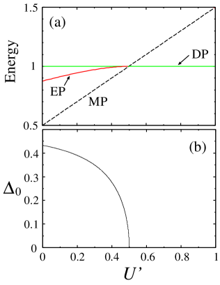
Figure 1: (a) Ground-state energies for EP and DP, and (b) $\Delta_{0}$ as functions of $U^{\prime}$ with $U=1$ and $\mu_{C}=0.5$. In (a), the energy of the magnetic phase (MP) is also shown by the dashed line.

Before the laser irradiation, we consider two phases in the ground state: an excitonic phase (EP) with $\Delta_{0}\neq 0$ and a decoupled phase (DP) with $\Delta_{0}=0$ and $n_{c}=0$. They correspond to EI and BI phases, respectively, when $t_{c}$ and $t_{f}$ are nonzero Kaneko_PRB12 ; Tanaka_PRB18 . We use $U=1$ and $\mu_{C}=0.5$, and vary $U^{\prime}$ ($\geq 0$) as a parameter. Since $\partial{E^{\rm AL}}/\partial{n_{c}}=0$ gives $n_{c}=1-\mu_{C}/(U-U^{\prime})$, we have a mean-field solution with $\Delta_{0}\neq 0$ for $0\leq U^{\prime}<U^{\prime}_{\rm cr}=U-\mu_{C}$. In Fig. 1(a), we show the ground-state energies for the EP and the DP, the latter of which is independent of $U^{\prime}$. With increasing $U^{\prime}$, a transition from the EP to the DP occurs at $U^{\prime}=U^{\prime}_{\rm cr}$. In fact, a magnetic phase (MP) with $\langle n^{c}_{\sigma}\rangle=1$ and $\langle n^{f}_{-\sigma}\rangle=1$ has the ground-state energy $U^{\prime}+\mu_{C}$, which becomes the lowest energy state for $0\leq U^{\prime}<U^{\prime}_{\rm cr}$. However, we consider only nonmagnetic initial states for the photoexcitation. The reason is that for nonzero $t_{c}$ and $t_{f}$, the photoinduced gap enhancement reported previously occurs in the vicinity of the boundary between the EI and BI phases Tanaka_PRB18 ($U^{\prime}\sim U^{\prime}_{\rm cr}$) where magnetic ordered states do not appear as the ground state Zocher_PRB11 . In this paper, we focus on the dynamics near $U^{\prime}=U^{\prime}_{\rm cr}$.

In Fig. 1(b), the $U^{\prime}$ dependence of $\Delta_{0}$ is shown, indicating that $\Delta_{0}$ is nonzero at $U^{\prime}=0$ and exhibits a steep decrease toward $U^{\prime}=U^{\prime}_{\rm cr}$ at which it vanishes. For $U^{\prime}\sim U^{\prime}_{\rm cr}$, this result is similar to that obtained with nonzero $t_{c}$ and $t_{f}$ (Fig. 10 in Sect. III B), whereas they are qualitatively different for $U^{\prime}\sim 0$. The similarity near $U^{\prime}=U^{\prime}_{\rm cr}$ comes from the local character of excitonic pairs: the EI is in the BEC regime of the BCS-BEC crossover Kaneko_PRB12 ; Phan_PRB10 ; Seki_PRB11 . On the other hand, for $U^{\prime}\sim 0$, the EI is in the BCS regime, which cannot be described by the atomic limit.

III.1.2 Photoinduced dynamics

In Fig. 2, we show the time evolutions of $n_{c}$ and $|\Delta_{0}|$ for different values of $F_{0}$ with $U^{\prime}=0.45$ ($<U^{\prime}_{\rm cr}$). For the time evolutions of the real and imaginary parts of $\Delta_{0}$, see Appendix A. We use $F(\tau)$ with the gaussian envelope [Eq. (3)] and choose $F_{0}<0$, although the sign of $F_{0}$ does not affect the results qualitatively Tanaka_PRB18 . The pump-light frequency is tuned to the difference between the two eigenvalues of Eq. (14) with $F(\tau)=0$. Since $n_{c}$ and $|\Delta_{0}|$ are conserved after the photoexcitation, they are denoted by $\widetilde{n_{c}}$ and $\widetilde{|\Delta_{0}|}$, respectively. As we increase $|F_{0}|$, $\widetilde{n_{c}}$ and $\widetilde{|\Delta_{0}|}$ become larger than those in the ground state. When $|F_{0}|$ is increased further ($|F_{0}|=0.6$), they are smaller than those at $\tau=0$. This behavior is qualitatively the same as that obtained in the previous study for the two-dimensional model near the EI-BI phase boundary Tanaka_PRB18 .

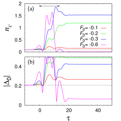
Figure 2: Time evolutions of (a) $n_{c}$ and (b) $|\Delta_{0}|$ for different values of $F_{0}$ with $U=1$, $\mu_{C}=0.5$, $U^{\prime}=0.45$, and $\omega=0.45$. The double-headed arrow indicates the range $0<\tau<2\tau_{w}=2\pi/\omega$ of application of an electric field. The horizontal dashed line in each panel indicates the corresponding equilibrium value.

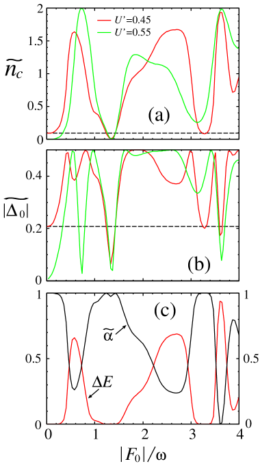
Figure 3: (a) $\widetilde{n_{c}}$, (b) $\widetilde{|\Delta_{0}|}$, and (c) $\Delta E$ and $\widetilde{\alpha}$ as functions of $|F_{0}|/\omega$ for $U=1$ and $\mu_{C}=0.5$. We use $F(\tau)$ with the gaussian envelope defined in Eq. (3). In (a) and (b), the results with $U^{\prime}=0.45$ and $0.55$ are shown, where the pump-light frequencies are $\omega=0.45$ and $\omega=0.6$, respectively. The dashed horizontal lines indicate the corresponding equilibrium values for $U^{\prime}=0.45$. For $U^{\prime}=0.55$, $n_{c}$ and $|\Delta_{0}|$ are zero in equilibrium. In (c), only the results with $U^{\prime}=0.45$ are shown.

In Figs. 3(a) and 3(b), we show $\widetilde{n_{c}}$ and $\widetilde{|\Delta_{0}|}$ as functions of $|F_{0}|/\omega$ for $U^{\prime}=0.45$ and $0.55$, where the ground states are in the EP and the DP, respectively. At time $\tau$, the wave function of the two-level system is written as

$$|\psi(\tau)\rangle=u(\tau)c^{\dagger}|0\rangle+v(\tau)f^{\dagger}|0\rangle,$$ (19)

with $|u(\tau)|^{2}+|v(\tau)|^{2}=1$ where we have omitted the spin index for brevity. By using the relations $n_{c}=2|u(\tau)|^{2}$ and $\Delta_{0}=u^{\ast}(\tau)v(\tau)$, we have

$$|\Delta_{0}|=\frac{1}{2}\sqrt{n_{c}(2-n_{c})},$$ (20)

which holds at any $\tau$ indicating that $\widetilde{|\Delta_{0}|}$ has its maximum value of $0.5$ when $\widetilde{n_{c}}=1$. In order to examine changes in the occupation probability of the two levels, we compute the overlap between the wave function in the ground state and that after the photoexcitation. The overlap $\alpha$ is given by

$$\alpha = |\langle\psi(\tau=0)|\psi(\tau)\rangle|^{2}$$ (21)

$$= 1-\frac{1}{2}(n_{c}+n^{G}_{c})+\frac{1}{2}n_{c}n^{G}_{c}+{\Delta_{0}^{G}}^{\ast}\Delta_{0}+\Delta_{0}^{G}{\Delta_{0}}^{\ast},$$

where $n^{G}_{c}$ and $\Delta_{0}^{G}$ are $n_{c}$ and $\Delta_{0}$ in the ground state, respectively. In evaluating $\alpha$, we adjust the phase of $\Delta_{0}$ in $|\psi(\tau=0)\rangle$ to coincide with that of $\Delta_{0}(\tau\neq 0)$. In this case, we have

$$\alpha=1-\frac{1}{2}(n_{c}+n^{G}_{c})+\frac{1}{2}n_{c}n^{G}_{c}+2|\Delta_{0}^{G}||\Delta_{0}|,$$ (22)

which is conserved after the photoexcitation. In Fig. 3(c), we show $\widetilde{\alpha}$ and the increment in the total energy $\Delta E$ per site for $U^{\prime}=0.45$. For the quantities $\widetilde{n_{c}}$, $\Delta E$, and $\widetilde{\alpha}$, an oscillatory behavior with respect to $|F_{0}|/\omega$ is evident, although the period of oscillation is not constant. The behavior of $\widetilde{|\Delta_{0}|}$ appears to be more complex than that of $\widetilde{n_{c}}$ because of the relation Eq. (20). The oscillation in $\widetilde{\alpha}$ and $\Delta E$ indicates a manifestation of the Rabi oscillation Rabi_PR37 ; Allen_BooK in the present two-level system, which we will discuss in detail below.

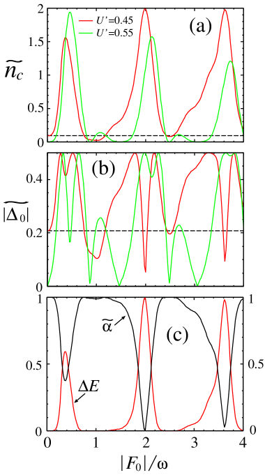
Figure 4: Same plots as Fig. 3 except that we use $F(\tau)$ with the rectangular envelope defined by Eq. (4).

III.1.3 Rabi oscillation and enhancement of excitonic order

Here we consider $F(\tau)$ with the rectangular envelope defined by Eq. (4). In Fig. 4, we show $\widetilde{n_{c}}$, $\widetilde{|\Delta_{0}|}$, $\Delta E$, and $\widetilde{\alpha}$ as functions of $|F_{0}|/\omega$ where the parameters are the same as those in Fig. 3. The oscillatory behavior of these quantities is more prominent than that in Fig. 3 where the gaussian envelope is employed for $F(\tau)$. In particular, the period of the oscillation is almost constant.

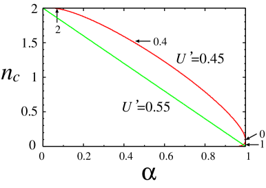
Figure 5: Relation between $\alpha$ and $n_{c}$ for $U^{\prime}=0.45$ and $0.55$. For $U^{\prime}=0.45$, the position $(\alpha,n_{c})$ at $|F_{0}|/\omega=0$ and $(\widetilde{\alpha},\widetilde{n_{c}})$ with $|F_{0}|/\omega=0.4$, $1$, and $2$ are depicted by the arrows.

By using Eqs. (20) and (22), we obtain the $\alpha$ dependence of $n_{c}$ shown in Fig. 5. Along its curve, the position $(\widetilde{\alpha},\widetilde{n_{c}})$ moves depending on the value of $|F_{0}|/\omega$. For $U^{\prime}=0.45$, we have $(\alpha,n_{c})=(1,0.091)$ in the ground state. With increasing $|F_{0}|/\omega$, the position ($\widetilde{\alpha}$, $\widetilde{n_{c}}$) first moves to the upper-left direction in Fig. 5 until $|F_{0}|/\omega\sim 0.4$ where $\widetilde{n_{c}}$ exhibits the first peak as shown in Fig. 4(a). Reflecting the periodic behavior of $\widetilde{\alpha}$, the point ($\widetilde{\alpha}$, $\widetilde{n_{c}}$) goes back to the initial position at $|F_{0}|/\omega\sim 0.8$. The value of $\widetilde{n_{c}}$ becomes smaller than $n^{G}_{c}$ for $0.8\lesssim|F_{0}|/\omega\lesssim 1.2$ [Fig. 4(a)] where $\widetilde{\alpha}$ is slightly smaller than 1 [Fig. 4(c)]. Then, ($\widetilde{\alpha}$, $\widetilde{n_{c}}$) moves to the upper-left direction again until $|F_{0}|/\omega=2.0$ at which $\widetilde{n_{c}}$ shows the second peak. For $U^{\prime}=0.55$, Eq. (22) gives $\alpha=1-\frac{1}{2}n_{c}$ since $n^{G}_{c}=\Delta^{G}_{0}=0$. The behavior of ($\widetilde{\alpha}$, $\widetilde{n_{c}}$) depending on $|F_{0}|/\omega$ is similar to that for $U^{\prime}=0.45$. These results show that the oscillatory behavior of physical quantities originates from that of $\widetilde{\alpha}$. In order to interpret our results as the Rabi oscillation more quantitatively, we consider the case of continuous-wave (CW) lasers in the following.

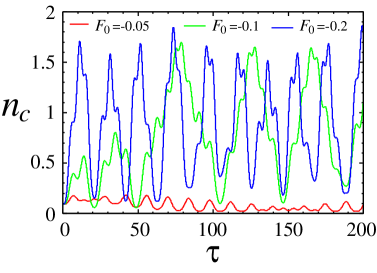
Figure 6: Time evolution of $n_{c}$ under CW excitations for different values of $F_{0}$. We use $U=1$, $\mu_{C}=0.5$, $U^{\prime}=0.45$, and $\omega=0.45$.

In Fig. 6, we show the time profile of $n_{c}$ under CW excitations for $U^{\prime}=0.45$ and $\omega=0.45$. When $|F_{0}|$ is small ($F_{0}=-0.05$), $n_{c}$ shows a small oscillation around the value of $n_{c}^{G}$. As we increase $|F_{0}|$, a large-amplitude oscillation appears, the period of which gets shorter for larger $|F_{0}|$.

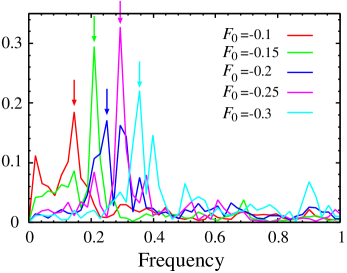
Figure 7: Fourier transform of $n_{c}$. In each spectrum, the position of its largest peak is indicated by the arrow. The parameters are the same as those in Fig. 6.

In Fig. 7, we show the Fourier transform of $n_{c}$ for large $|F_{0}|$ ($F_{0}\leq-0.1$) (see Appendix A for the details of the dynamics for small $|F_{0}|$). There is a sharp peak in each spectrum and its position denoted by $\Omega$ is nearly proportional to $|F_{0}|$ as shown in Fig. 8. In a two-level system driven by a CW laser, the rotating wave approximation (RWA) gives the Rabi frequency $\Omega_{R}$ as

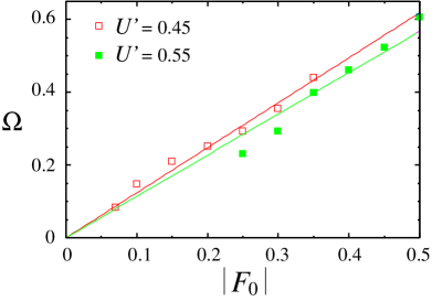
Figure 8: Peak frequency $\Omega$ in Fourier transform of $n_{c}$ as a function of $|F_{0}|$ for $U^{\prime}=0.45$ and $0.55$. The solid lines are fitting results.

$$\Omega_{R}=\sqrt{(\omega-E_{G})^{2}+{F_{0}}^{2}},$$ (23)

where $E_{G}$ is the difference between the two energy levels. At the resonance ($\omega=E_{G}$), we have $\Omega_{R}=|F_{0}|$. In fact, the Hamiltonian in Eq. (14) contains $n_{c}$ and $\Delta_{0}$ that are $\tau$ dependent, which is different from the conventional Rabi oscillation Rabi_PR37 ; Allen_BooK . The effects of the $\tau$-dependence of $n_{c}$ and $\Delta_{0}$ in the Hamiltonian on the dynamics are discussed in Appendix B. Considering this difference, here we will replace $\Omega_{R}$ at the resonance [$\omega=E_{G}(\tau=0)$] by $\Omega^{\prime}_{R}=p|F_{0}|$ with a coefficient $p$ Ono_PRB16 . This leads us to $u(\tau)\propto\sin(\frac{\Omega^{\prime}_{R}}{2}\tau+\phi)$

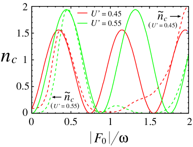
Figure 9: $|F_{0}|/\omega$ dependence of $n_{c}$ obtained by Eq. (24) at $\tau=2\pi/\omega$. We show $\widetilde{n_{c}}$ in Fig. 4(a) by the dashed lines for comparison. We use $U^{\prime}=0.45$ and $0.55$.

so that $n_{c}$ is written as

$$n_{c}=A\sin^{2}(\frac{\Omega^{\prime}_{R}}{2}\tau+\phi),$$ (24)

where $A$ and $\phi$ are constants. We fit a linear function $\Omega=p|F_{0}|$ to the results of $\Omega$ in Fig. 8. The fitting works well with $p$ slightly larger than $1$ for both $U^{\prime}=0.45$ ($p=1.24$) and $0.55$ ($p=1.14$). In Eq. (24), we have $\phi\sim 0$ ($\phi=0$) when $U^{\prime}$ is slightly smaller (larger) than $U^{\prime}_{\rm cr}$ because of $n^{G}_{c}\sim 0$ ($n^{G}_{c}=0$), indicating that for single cycle pulses the values of $n_{c}$ and $|\Delta_{0}|$ after the photoexcitation are governed by $\Omega^{\prime}_{R}/\omega$. In particular, $n_{c}$ becomes maximum at $\Omega^{\prime}_{R}/\omega\sim 1/2$. This relation gives $|F_{0}|/\omega=0.40$ for $U^{\prime}=0.45$ and $|F_{0}|/\omega=0.44$ for $U^{\prime}=0.55$, which are consistent with the results shown in Fig. 4(a). In Fig. 9, we show the $|F_{0}|/\omega$ dependence of $n_{c}$ calculated by Eq. (24) at $\tau=2\pi/\omega$, and compare the result with $\widetilde{n_{c}}$ shown in Fig. 4(a). The quantities $A$ and $\phi$ are determined from the height of the first peak in $\widetilde{n_{c}}$ and the value of $n^{G}_{c}$. For $|F_{0}|/\omega\lesssim 0.8$, the results obtained by Eq. (24) reproduce those for $\widetilde{n_{c}}$ fairly well, although they deviate from each other for larger $|F_{0}|/\omega$, which is due to the limitation of the RWA Nishioka_JPSJ14 .

III.2 One-dimensional model

Next, we show results for the one-dimensional model with $t_{f}=1$ and $t_{c}=-1$ in Eq. (1), for which the initial EI and BI have a direct gap Tanaka_PRB18 .

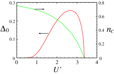
Figure 10: $\Delta_{0}$ and $n_{c}$ as functions of $U^{\prime}$ with $U=4$ and $\mu_{C}=2.5$.

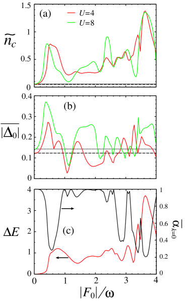
Figure 11: (a) $\widetilde{n_{c}}$ and (b) $\overline{|\Delta_{0}|}$ as functions of $|F_{0}|/\omega$ for $U=4$ and $U=8$. We use $F(\tau)$ with the gaussian envelope. For $U=4$ ($U=8$), we set $U^{\prime}=3.3$ and $\mu_{c}=2.5$ ($U^{\prime}=4.3$ and $\mu_{c}=5$). The dashed (dotted) horizontal lines indicate the corresponding equilibrium values for $U=4$ ($U=8$). (c) $\Delta E$ and $\overline{\alpha}_{k=0}$ as functions of $|F_{0}|/\omega$ for $U=4$.

III.2.1 Ground state

In Fig. 10, we show $\Delta_{0}$ and $n_{c}$ as functions of $U^{\prime}$ in the ground state with $U=4$ and $\mu_{C}=2.5$. As in the previous studies where the Fermi surface is perfectly nested Kaneko_PRB12 ; Tanaka_PRB18 , an infinitesimal $U^{\prime}$ produces an EI with $\Delta_{0}\neq 0$. The order parameter $\Delta_{0}$ exhibits a maximum at $U^{\prime}=2.70$ and a transition from the EI to BI phases occurs at $U^{\prime}=U^{\prime}_{\rm cr}=3.37$ where $\Delta_{0}$ vanishes. Toward $U^{\prime}=U^{\prime}_{\rm cr}$, $n_{c}$ monotonically decreases. In the BI phase, the $c$ and $f$ bands are completely decoupled so that we have $\Delta_{0}=0$ and $n_{c}=0$ ($n_{f}=2$).

III.2.2 Photoinduced dynamics

In the calculations of photoinduced dynamics, we use two sets of parameters, both of which give EIs that are located near the EI-BI phase boundary of the ground states. One is $U=4$, $\mu_{C}=2.5$ and $U^{\prime}=3.3$. The other is $U=8$, $\mu_{C}=5$ and $U^{\prime}=4.3$ where $U^{\prime}_{\rm cr}=4.5$. We use $F(\tau)$ with the gaussian envelope [Eq. (3)] and the pump-light frequency is tuned to the initial gap of the EI: $\omega=1.25$ for $U=4$ and $\omega=1.99$ for $U=8$. We note that as far as $U^{\prime}\sim U^{\prime}_{\rm cr}$, our results are qualitatively unaltered even when we choose a BI as the initial state. The system size is $N=200$. In analogy with the case of the atomic limit, we define a $k$-dependent quantity $\alpha_{k}$ as follows. First, we consider the overlap between the one-particle state at time $\tau$ and that in the ground state. If we write the one-particle state as $|\psi_{k\sigma}(\tau)\rangle=u_{k\sigma}(\tau)c^{\dagger}_{k\sigma}|0\rangle+v_{k\sigma}(\tau)f^{\dagger}_{k\sigma}|0\rangle$ with $|u_{k\sigma}|^{2}+|v_{k\sigma}|^{2}=1$, the overlap is written as

$$|\langle\psi_{k\sigma}(\tau=0)|\psi_{k\sigma}(\tau)\rangle|^{2}$$ (25)

$$= n_{c}^{G}(k)n_{c}(k)+[1-n_{c}^{G}(k)][1-n_{c}(k)]$$

$$+ {\Delta^{G}}^{\ast}(k)\Delta(k)+{\Delta^{G}}(k)\Delta^{\ast}(k),$$

where ${n_{c}}(k)$ and $\Delta(k)$ are the momentum distribution function for $c$-electrons and the pair amplitude in $k$ space, which are written as

$$n_{c}(k)=\langle c^{\dagger}_{k\sigma}c_{k\sigma}\rangle=|u_{k\sigma}|^{2},$$ (26)

and

$$\Delta(k)=\langle c^{\dagger}_{k\sigma}f_{k\sigma}\rangle={u_{k\sigma}}^{\ast}v_{k\sigma},$$ (27)

respectively, and $n_{c}^{G}(k)$ [$\Delta^{G}(k)$] is $n_{c}(k)$ [$\Delta(k)$] in the ground state. Then, as in Eq. (22), we define $\alpha_{k}$ as

$$\alpha_{k} = n_{c}^{G}(k)n_{c}(k)+[1-n_{c}^{G}(k)][1-n_{c}(k)]$$ (28)

$$+ 2|{\Delta^{G}}(k)||\Delta(k)|,$$

which is the upper limit of the overlap in Eq. (25).

After the photoexcitation, $n_{c}$ is conserved and it is denoted by $\widetilde{n_{c}}$, whereas the time profile of $|\Delta_{0}|$ exhibits an oscillation corresponding to the Higgs amplitude mode Tanaka_PRB18 . The time average of $|\Delta_{0}|$ is denoted by $\overline{|\Delta_{0}|}$, which is defined in Eq. (10). In Fig. 11, we show $\widetilde{n_{c}}$, $\overline{|\Delta_{0}|}$, $\Delta E$, and $\overline{\alpha}_{k=0}$ (denoting the time average of $\alpha_{k=0}$) as functions of $|F_{0}|/\omega$, where $k=0$ is the location of the gap in the ground state. The time average is taken with $\tau_{i}=20$ and $\tau_{f}=50$. For $|F_{0}|/\omega\lesssim 1$, the $|F_{0}|/\omega$ dependence of these quantities is similar to that in the atomic limit shown in Fig. 3, indicating that the dynamics are qualitatively described by the Rabi oscillation even when the bands are formed. As shown in Fig. 11(a), $\widetilde{n_{c}}$ has a peak at $|F_{0}|/\omega\simeq 0.5$ which is comparable to the case of the atomic limit [Fig. 3(a)]. For large $|F_{0}|$ ($|F_{0}|/\omega\gtrsim 1$), a cyclic behavior of physical quantities that characterizes the Rabi oscillation becomes less clear. When we employ the rectangular envelope for $F(\tau)$, the cyclic behavior appears even in the region of large $|F_{0}|/\omega$ (Fig. 13).

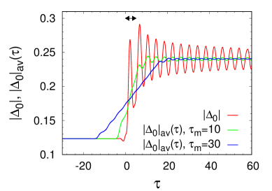
Figure 12: Time profiles of $|\Delta_{0}|$ and $|\Delta_{0}|_{\rm av}(\tau)$. We use $\tau_{m}=10$ and $30$ for $|\Delta_{0}|_{\rm av}(\tau)$. The other parameters are $U=4$, $U^{\prime}=3.3$, $\mu_{C}=2.5$, $\omega=1.25$, and $F_{0}=-0.5$. The double-headed arrow indicates the range $0<\tau<2\tau_{w}$ of application of an electric field.

Here we mention the choice of the values of $\tau_{i}$ and $\tau_{f}$ in Eq. (10). After the photoexcitations, physical quantities generally show oscillations in time. In the time-dependent HF method, the center of such an oscillation is almost constant because dephasing processes via electron correlations are not taken into account. In Fig. 12, we show the time profile of $|\Delta_{0}|$ where we use the $U=4$, $U^{\prime}=3.3$, $\mu_{C}=2.5$, $\omega=1.25$, and $F_{0}=-0.5$, which gives a large enhancement of $|\Delta_{0}|$. After the photoexcitation, $|\Delta_{0}|$ exhibits the Higgs amplitude mode with a period of about $4.0$, whereas the center of its oscillation is almost constant. In order to show explicitly how the values of $\tau_{i}$ and $\tau_{f}$ affect the time average, we define the time average of a physical quantity $X(\tau)$ taken in the range from $\tau-\tau_{m}/2$ to $\tau+\tau_{m}/2$ as,

$$X_{\rm av}(\tau)=\frac{1}{\tau_{m}}\int^{\tau+\tau_{m}/2}_{\tau-\tau_{m}/2}X(\tau^{\prime})d\tau^{\prime}.$$ (29)

The time profiles of $|\Delta_{0}|_{\rm av}(\tau)$ with $\tau_{m}=10$ and $30$ are shown in Fig. 12, which indicates that their difference is very small for $\tau>20$. We note that $\overline{|\Delta_{0}|}$ with $\tau_{i}=20$ and $\tau_{f}=50$ presented in Fig. 11(b) corresponds to $|\Delta_{0}|_{\rm av}(\tau)$ with $\tau_{m}=30$ at $\tau=35$. From these results, we confirm that, when $\tau_{m}=\tau_{f}-\tau_{i}$ is larger than the oscillation period of $|\Delta_{0}|$ and $\tau_{i}$ is taken sufficiently after the photoexcitation, the value of $\tau_{m}$ has little effects on the results. For the relevance to experiments, if we use $t_{f}=0.4$ eV for Ta₂NiSe₅ Seki_PRB14 , $\tau_{f}-\tau_{i}=30$ corresponds to 50 fs, which is comparable to time resolution of recent pump-probe measurements Mor_PRL17 . When $|\Delta_{0}|$ is small after the photoexcitation, the period of the Higgs mode may become long. However, in such cases the amplitude of the Higgs mode becomes small and thus the choice of $\tau_{i}$ and $\tau_{f}$ does not largely affect the results.

III.2.3 Signature of Rabi oscillation in one-particle states

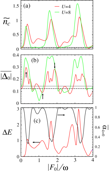
Figure 13: Same plots as Fig. 11 except that we use $F(\tau)$ with the rectangular envelope. In (b), the positions of $\overline{|\Delta_{0}|}$ with $|F_{0}|/\omega=0.3$, $1.2$, and $1.9$ for $U=4$ are indicated by the arrows.

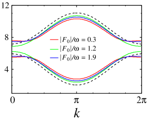
Figure 14: $\overline{E}_{k\gamma\sigma}$ for different values of $|F_{0}|/\omega$. The dashed lines show the energy levels in the ground state. The parameters are $U=4$, $\mu_{C}=2.5$, and $U^{\prime}=3.3$.

Here we consider $F(\tau)$ with the rectangular envelope [Eq. (4)]. As in the case of the atomic limit, we discuss our results from the viewpoint of the Rabi oscillation. In Fig. 13, we show $\widetilde{n_{c}}$, $\overline{|\Delta_{0}|}$, $\Delta E$, and $\overline{\alpha}_{k=0}$ as functions of $|F_{0}|/\omega$. The oscillatory behavior in these quantities is more evident than that in Fig. 11 where the gaussian envelope is employed for $F(\tau)$. General tendencies of Figs. 13(a), 13(b), and 13(c) are similar to those of Figs. 4(a), 4(b), and 4(c), respectively. This means that if we apply Eq. (24) to the case of nonzero transfer integrals, the value of $p$ is almost unchanged from that in the atomic limit. Compared to the results with $U=4$, the oscillatory behavior is more prominent for those with $U=8$ where the system is closer to the atomic limit.

In Fig. 14, the time averages of the transient energy levels, $\overline{E}_{k\gamma\sigma}$, with $\gamma$ being the band index, are shown for $U=4$. The transient energy levels $E_{k\gamma\sigma}(\tau)$ are obtained by diagonalizing Eq. (8). We use $|F_{0}|/\omega=0.3$, $1.2$, and $1.9$, for which the values of $\overline{|\Delta_{0}|}$ are indicated by the arrows in Fig. 13(b). For $|F_{0}|/\omega=0.3$ and $1.9$, the gap in $\overline{E}_{k\gamma\sigma}$ is larger than that in the ground state because of the enhancement of $\overline{|\Delta_{0}|}$, whereas it becomes smaller for $|F_{0}|/\omega=1.2$ where $\overline{|\Delta_{0}|}$ is suppressed.

Since the one-particle Hamiltonian is described by a $2\times 2$ matrix, we can expect that the Rabi oscillation occurs for each $k$. In order to confirm this, in Fig. 15(a) we show $\overline{\alpha}_{k}$ on the $(|F_{0}|/\omega,k)$ plane for $U=4$. It is apparent that $\overline{\alpha}_{k}$ exhibits an oscillation with respect to $|F_{0}|/\omega$. The oscillation amplitude depends on $k$ and is large around $k=0$ that is the location of the initial gap, whereas the period of oscillation is nearly independent of $k$. As shown in Fig. 13, the periodic behavior of $\overline{\alpha}_{k=0}$ with respect to $|F_{0}|/\omega$ corresponds to those in $\widetilde{n_{c}}$, $\overline{|\Delta_{0}|}$, and $\Delta E$. By using Eqs. (26) and (27), we have

$$|\Delta(k)|=\sqrt{n_{c}(k)(1-n_{c}(k))},$$ (30)

from which the relation between $\alpha_{k}$ and $n_{c}(k)$ is obtained, as shown in Fig. 15(b) for the case of $k=0$. A similar relation is obtained even if we choose another $k$ (not shown). In the figure, we depict ($\alpha_{k=0},n_{c}(0)$) in the ground state and ($\overline{\alpha}_{k=0},\overline{n_{c}(0)}$) for $|F_{0}|/\omega=0.3$, $1.2$, and $1.9$. The periodic change in the position as a function of $|F_{0}|/\omega$ is similar to that in the atomic limit discussed in Sect. III A. These results show that the periodic behavior of $\overline{\alpha}_{k}$ brings about that of $\overline{n_{c}(k)}$. Thus, the $|F_{0}|/\omega$ dependence of physical quantities is essentially caused by the Rabi oscillation of each one-particle state.

In order to understand the $|F_{0}|/\omega$ dependence of $\overline{|\Delta_{0}|}$ in Fig. 13(b) more accurately, it is necessary to discuss the phase of $\Delta(k)$ as well as the $k$ dependence of $n_{c}(k)$ and $\Delta(k)$. They have been shown to have an important role in determining whether the photoinduced enhancement of the excitonic gap occurs Tanaka_PRB18 . The order parameter $\Delta_{0}$ is related with $\Delta(k)$ by

$$\Delta_{0}=\frac{1}{N}\sum_{k}\Delta(k),$$ (31)

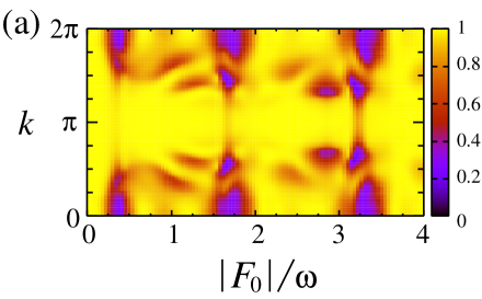
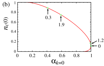
Figure 15: (a) $\overline{\alpha}_{k}$ on $(|F_{0}|/\omega,k)$ plane. (b) Relation between $\alpha_{k=0}$ and $n_{c}(0)$. The position ($\alpha_{k=0},n_{c}(0)$) in the ground state and ($\overline{\alpha}_{k=0},\overline{n_{c}(0)}$) with $|F_{0}|/\omega=0.3$, $1.2$, and $1.9$ are indicated by the arrows. We use $U=4$, $\mu_{C}=2.5$, and $U^{\prime}=3.3$.

and we define their phases as

$$\Delta(k)=|\Delta(k)|e^{i\theta_{k}},$$ (32)

and

$$\Delta_{0}=|\Delta_{0}|e^{i\theta}.$$ (33)

In Fig. 16, we show $\overline{n_{c}(k)}$, $\overline{|\Delta(k)|}$, and $\overline{\delta\theta}_{k}$ for $|F_{0}|/\omega=0.3$, $1.2$, and $1.9$, where $\delta\theta_{k}$ is defined as

$$\delta\theta_{k}=\left\{\begin{array}[]{ll}|\theta_{k}-\theta|&(|\theta_{k}-\theta|<\pi)\\ |\theta_{k}-\theta|-\pi&({\rm otherwise}).\end{array}\right.$$ (34)

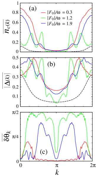
Figure 16: (a) $\overline{n_{c}(k)}$, (b) $\overline{|\Delta(k)|}$, and (c) $\overline{\delta\theta}_{k}$ for different values of $|F_{0}|/\omega$. The dashed lines are the corresponding equilibrium values. The parameters are $U=4$, $\mu_{C}=2.5$, and $U^{\prime}=3.3$.

In the ground state, $n_{c}(k)$ and $\Delta(k)$ have a broad $k$ dependence because of the BEC nature of the excitonic condensation. After the photoexcitation, $\overline{n_{c}(k)}$ and $\overline{|\Delta(k)|}$ are basically increased compared to their ground-state values. From Eq. (30), $|\Delta(k)|$ has its maximum value of $0.5$ when $n_{c}(k)=0.5$. When $\widetilde{n_{c}}$ is increased by the increase in $\overline{n_{c}(k)}$, the mixing between the upper and lower bands is promoted and $\overline{|\Delta(k)|}$ is enhanced Tanaka_PRB18 . However, this does not necessarily bring about the enhancement of $\overline{|\Delta_{0}|}$. When $|F_{0}|/\omega=1.2$, for instance, $\overline{|\Delta_{0}|}$ is smaller than $\Delta^{G}_{0}$ [Fig. 13(b)] although $\widetilde{n_{c}}$ is larger than $n^{G}_{c}$ [Fig. 13(a)]. As shown in Fig. 16(c), $\overline{\delta\theta}_{k}$ is large in a wide region of the Brillouin zone, indicating that the enhancement of $\overline{|\Delta_{0}|}$ is hindered by the large deviation of $\theta_{k}$ from $\theta$. On the other hand, for $|F_{0}|/\omega=0.3$, $\theta_{k}$ is in phase with $\theta$ in a large area in $k$ space. For $|F_{0}|/\omega=1.9$, although $\overline{\delta\theta}_{k}$ becomes large near $k=\pm 0.6\pi$, it is small for $|k|\lesssim 0.4\pi$ where $\overline{|\Delta(k)|}$ has its maximum. Therefore, the increase in $\overline{|\Delta(k)|}$ leads to the enhancement of $\overline{|\Delta_{0}|}$. In short, when $\overline{|\Delta_{0}|}$ is enhanced by photoexcitation, $\theta_{k}$ is in phase with $\theta$ in a region where $\overline{|\Delta(k)|}$ is largely increased, whereas $\theta_{k}$ behaves differently from $\theta$ when $\overline{|\Delta_{0}|}$ is suppressed. In the former, the Rabi oscillations of one-particle states with different $k$ values work cooperatively to induce the gap enhancement.

As we have shown in the previous paper Tanaka_PRB18 , when $U^{\prime}$ is small and the initial EI is of BCS type, the time evolution of $\theta_{k}$ induces a destructive interference to hinder the enhancement of $|\Delta_{0}|$, which is also the case for $U^{\prime}=0$. Since the excitonic order for small $U^{\prime}$ has a long correlation length, its photoinduced dynamics cannot be understood in terms of the Rabi oscillation in the atomic limit. However, when the initial state is of BEC type, the phases $\theta_{k}$ are nearly in phase and the Rabi oscillations for different $k$ values work cooperatively to enhance $|\Delta_{0}|$.

IV Effects of Electron-Phonon Coupling

We investigate effects of phonons on the photoinduced dynamics within the HF approximation. We consider the additional terms to Eq. (1), which are used in Murakami_PRL17 ,

$$\hat{H}_{\rm eph} = g\sum_{i\sigma}(b_{i}+b^{\dagger}_{i})(c^{\dagger}_{i\sigma}f_{i\sigma}+f^{\dagger}_{i\sigma}c_{i\sigma}),$$ (35)

$$\hat{H}_{\rm p} = \omega_{p}\sum_{i}b^{\dagger}_{i}b_{i},$$ (36)

where $b_{i}$ ($b^{\dagger}_{i}$) is the annihilation (creation) operator for the phonon at the $i$th site. The e-ph coupling constant and the phonon frequency are denoted by $g$ and $\omega_{p}$, respectively. We define the expectation value of the lattice displacement, $y_{p}=\langle b_{i}\rangle+\langle b^{\dagger}_{i}\rangle$, which is assumed to be independent of $i$. The time evolution of the system is computed as follows Tanaka_JPSJ10 . For phonons, we treat them as classical variables and numerically solve the equation of motion for $y_{p}$ that is written as

$$\frac{d^{2}y_{p}}{dt^{2}}=-\omega_{p}^{2}y_{p}-8g\omega_{p}{\rm Re}\Delta_{0},$$ (37)

from which we have

$$y_{p}=-\frac{8g}{\omega_{p}}{\rm Re}\Delta_{0},$$ (38)

in the ground state. For the electronic part, we employ Eq. (9). In this section, we use $F(\tau)$ with the gaussian envelope [Eq. (3)]. The results obtained by the rectangular envelope are given in Appendix C.

IV.1 Atomic limit

First, we discuss the case of the atomic limit ($t_{f}=t_{c}=0$). In the ground state, we can show that Eq. (20) holds even in the presence of the e-ph interaction. From Eqs. (20) and (38), the ground-state energy $E^{\rm AL}_{g}$ is written as

$$E^{\rm AL}_{g}=\frac{1}{2}(U-U^{\prime}_{g})n_{c}^{2}+(\mu_{C}-U+U^{\prime}_{g})n_{c}+U,$$ (39)

where $U^{\prime}_{g}=U^{\prime}-8g^{2}/\omega_{p}$. This leads to $n_{c}=1-\mu_{C}/(U-U^{\prime}_{g})$ and the critical value of $U^{\prime}$ for the EP-DP phase boundary is given by $U^{\prime}_{\rm cr}=U-\mu_{C}+8g^{2}/\omega_{p}$. In Fig. 17, we show the time average of $n_{c}$, which is denoted by $\overline{n_{c}}$, as a function of $|F_{0}|/\omega$ for $g=0.01$ and $g=0.02$ with $U=1$, $U^{\prime}=0.45$, $\mu_{C}=0.5$, and $\omega_{p}=0.1$. For $g=0.01$ ($g=0.02$), we have $U^{\prime}_{\rm cr}=0.508$ ($U^{\prime}_{\rm cr}=0.532$). The value of $\omega$ is so chosen that it corresponds to the energy difference between the two levels. The time average is taken with $\tau_{i}=100$ and $\tau_{f}=400$ considering the long time-scale of phonons, $2\pi/\omega_{p}$.

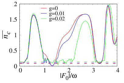
Figure 17: $\overline{n_{c}}$ as a function of $|F_{0}|/\omega$ for different values of $g$ with $U=1$, $U^{\prime}=0.45$ and $\mu_{C}=0.5$ in the atomic limit. We use $\omega=0.45$, $0.458$, and $0.482$ for $g=0$, $0.01$, and $0.02$, respectively. The horizontal dashed lines indicate the corresponding equilibrium values.

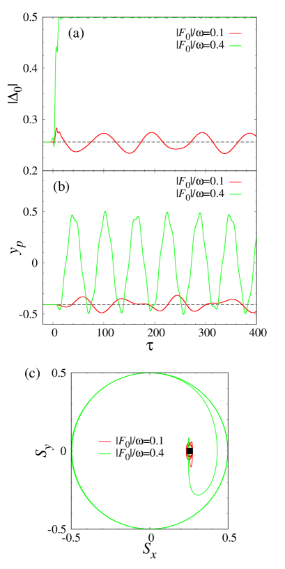
Figure 18: Time evolutions of (a) $|\Delta_{0}|$ and (b) $y_{p}$, and (c) trajectory of $(S_{x},S_{y})$ for $|F_{0}|/\omega=0.1$ and $0.4$. We use $g=0.02$ and the other parameters are the same as those in Fig. 17. In (a) and (b), the horizontal lines indicate the corresponding equilibrium values. In (c), we depict the time domain $-20\leq\tau\leq 300$ ($-20\leq\tau\leq 50$) for $|F_{0}|/\omega=0.1$ ($|F_{0}|/\omega=0.4$), and the solid square indicates the initial position of $(S_{x},S_{y})$.

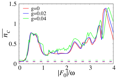
Figure 19: $\overline{n_{c}}$ as a function of $|F_{0}|/\omega$ for different values of $g$ with $U=4$, $U^{\prime}=3.3$, and $\mu_{C}=2.5$ for the case of nonzero transfer integrals ($t_{f}=-t_{c}=1$). We use $\omega=1.25$, $1.30$, and $1.42$ for $g=0$, $0.02$, and $0.04$, respectively. The horizontal dashed lines indicate the corresponding equilibrium values.

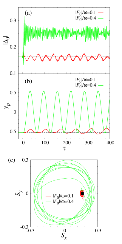
Figure 20: Time evolutions of (a) $|\Delta_{0}|$ and (b) $y_{p}$, and (c) trajectory of $(S_{x},S_{y})$ for $|F_{0}|/\omega_{0}=0.1$ and $0.4$. We use $g=0.04$ and the other parameters are the same as those in Fig. 19. In (a) and (b), the horizontal lines indicate the corresponding equilibrium values. In (c), we depict the time domain $-20\leq\tau\leq 300$ ($-20\leq\tau\leq 50$) for $|F_{0}|/\omega=0.1$ ($|F_{0}|/\omega=0.4$), and the solid square indicates the initial position of $(S_{x},S_{y})$.

It is apparent that the Rabi oscillation appears even with nonzero $g$. We note that this is also the case when we use the rectangular envelope for $F(\tau)$ (Appendix C). For $g=0.02$, we depict the time profiles of $|\Delta_{0}|$ and $y_{p}$ in Figs. 18(a) and 18(b), respectively. When $|F_{0}|$ is small ($|F_{0}|/\omega=0.1$), $|\Delta_{0}|$ and $y_{p}$ oscillate around their ground-state values. However, for large $|F_{0}|$ ($|F_{0}|/\omega=0.4$), $|\Delta_{0}|$ is enhanced and $y_{p}$ oscillates around zero indicating that the effect of the lattice displacement basically disappears. In Fig. 18(c), we show the trajectory of $(S_{x},S_{y})$ where we define $S_{x}={\rm Re}\Delta_{0}$ and $S_{y}={\rm Im}\Delta_{0}$ in the pseudospin representation. The description of the pseudospin representation and the trajectory of $(S_{x},S_{y})$ for $g=0$ are given in Appendix A. For small $|F_{0}|$, $\theta$ that is defined in Eq. (33) is confined near zero. This is because the phase mode is massive in the presence of the lattice displacement Murakami_PRL17 . On the other hand, $\theta$ rotates for large $|F_{0}|$, which is qualitatively the same as that for $g=0$ (Fig. 28 in Appendix A).

IV.2 One-dimensional model

Next, we show results with nonzero transfer integrals ($t_{f}=-t_{c}=1$). We compute $\overline{n_{c}}$ as a function of $|F_{0}|/\omega$ for $g=0.02$ and $0.04$ where the lattice displacements in the ground state are $y_{p}=-0.217$ and $y_{p}=-0.527$, respectively. Here we use $U=4$, $U^{\prime}=3.3$, and $\mu_{C}=2.5$. The used value of $\omega$ corresponds to the initial gap. As shown in Fig. 19, the introduction of the e-ph coupling does not largely affect the $|F_{0}|/\omega$ dependence of $\overline{n_{c}}$ as in the case of the atomic limit. For $g=0.04$, we show the time profiles of $|\Delta_{0}|$ and $y_{p}$ in Figs. 20(a) and 20(b), respectively, whereas the trajectory of $(S_{x},S_{y})$ is shown in Fig. 20(c). We use $|F_{0}|/\omega=0.1$ ($\overline{|\Delta_{0}|}/\Delta_{0}(\tau=0)=0.97$) and $|F_{0}|/\omega=0.4$ ($\overline{|\Delta_{0}|}/\Delta_{0}(\tau=0)=1.53$). The results are qualitatively the same as those in the atomic limit shown in Fig. 18. These results indicate that the e-ph coupling does not have a significant role on the photoinduced gap enhancement based on the Rabi oscillation.

V Correlation effects

In this section, we examine effects of the electron correlation that are ignored in the HF approximation. By using the ED method, we calculate ground-state properties and photoinduced dynamics of the two-orbital Hubbard model. We do not consider the e-ph coupling for simplicity. When we use single cycle pulses for photoexcitations, we adopt $F(\tau)$ with the gaussian envelope and the results obtained with the rectangular envelope are given in Appendix D.

V.1 Ground state

In the ground state, we compute the $U^{\prime}$ dependence of $n_{c}$ where we use $U=4$, $\mu_{C}=2.5$ and the system size $N=6$. As shown in Fig. 21, $n_{c}$ monotonically decreases with increasing $U^{\prime}$ and it becomes zero at $U_{\rm cr}^{\prime}=3.5$. This behavior is consistent with the HF results shown in Fig. 10 where we have $U_{\rm cr}^{\prime}=3.37$. The qualitative difference between the HF and ED results is that for $U^{\prime}<U_{\rm cr}^{\prime}$ the excitonic order parameter $\Delta_{0}$ is nonzero in the former whereas it is zero in the latter. We note that by the ED method we inevitably have a ground state with $\Delta_{0}=0$ because of the finiteness of the system. For $U^{\prime}>U_{\rm cr}^{\prime}$, both methods give the BI phase with $\Delta_{0}=n_{c}=0$ as the ground state. In this phase, the gap $E_{1}-E_{0}$ increases almost linearly with $U^{\prime}$ as shown in Fig. 21, where $E_{0}$ and $E_{1}$ are the energies of the ground and first excited states, respectively. This behavior is also consistent with the HF results Tanaka_PRB18 . In the following, we consider the BI phase ($U^{\prime}>U^{\prime}_{\rm cr}$) as the initial state before photoexcitation for comparison.

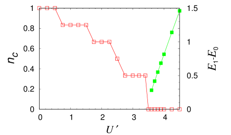
Figure 21: $n_{c}$ as a function of $U^{\prime}$ with $U=4$, $\mu_{C}=2.5$, and $N=6$. We also show the gap $E_{1}-E_{0}$ for $U^{\prime}>U^{\prime}_{\rm cr}$.

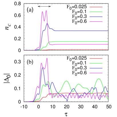
Figure 22: Time evolutions of (a) $n_{c}$ and (b) $|\Delta_{0}|$ for different values of $F_{0}$ obtained by the ED method with $U=4$, $\mu_{C}=2.5$, $U^{\prime}=3.9$, $\omega=0.7$, and $N=6$. The double-headed arrow in (a) indicates the range $0<\tau<2\tau_{w}=2\pi/\omega$ of application of an electric field.

V.2 Photoinduced dynamics

The time evolution of the system is obtained by numerically solving the time-dependent Schr$\ddot{\rm o}$dinger equation for the exact many-electron wave function $|\Psi(\tau)\rangle$ as

$$|\Psi(\tau+d\tau)\rangle=\exp\Bigl{[}-id\tau\hat{H}_{\rm tot}\Bigl{(}\tau+\frac{d\tau}{2}\Bigr{)}\Bigr{]}|\Psi(\tau)\rangle,$$ (40)

where $\hat{H}_{\rm tot}(\tau)=\hat{H}+\hat{H}_{D}(\tau)$ and we use $d\tau=0.01$. We use $U=4$, $\mu_{C}=2.5$, and $U^{\prime}=3.9>U^{\prime}_{\rm cr}$. The light frequency is set at $\omega=0.7$ that is near the gap $E_{1}-E_{0}=0.68$. In the following, we first show results with single cycle pulses and then discuss the case of CW excitations.

V.2.1 Excitations with single cycle pulse

In Fig. 22, we show the time profiles of $n_{c}$ and $|\Delta_{0}|$ for different values of $F_{0}$ with $0<F_{0}/\omega\lesssim 1$. After the photoexcitation, $n_{c}$ is conserved, whereas $|\Delta_{0}|$ keeps oscillating. The value of $\widetilde{n_{c}}$ increases with increasing $F_{0}$, and then it decreases when we increase $F_{0}$ further ($F_{0}=0.6$). As shown in Fig. 22(b), there is no clear indication of a strong dephasing in the order parameter that should suppress $|\Delta_{0}|$ after the photoexcitation with $0<F_{0}/\omega\lesssim 1$. Moreover, we do not find rapid thermalization: the oscillation in $|\Delta_{0}|$ persists long after the photoexcitation with $0<F_{0}/\omega\lesssim 1$. Although the finite size effects may play a role, our results at this stage do not indicate that the correlation effects seriously hinder the enhancement of $|\Delta_{0}|$. We depict $\widetilde{n_{c}}$, $\overline{|\Delta_{0}|}$, $\Delta E$ and $\widetilde{\alpha}$ as functions of $F_{0}/\omega$ in Fig. 23 where the time average of $|\Delta_{0}|$ is taken with $\tau_{i}=50$ and $\tau_{f}=100$. Here the overlap $\alpha$ is defined by $\alpha=|\langle\Psi(\tau)|\Psi(0)\rangle|^{2}$. After the photoexcitation, $\alpha$ is conserved and its value is denoted by $\widetilde{\alpha}$. Notably, our results indicate that for $F_{0}/\omega\lesssim 1$, the $F_{0}/\omega$ dependence of these quantities is consistent with that obtained by the HF method shown in Fig. 11. This strongly suggests that the enhancement of $|\Delta_{0}|$ as well as its interpretation with the help of the Rabi oscillation are robust against the correlation effects. We note that although the ED calculations are limited to small system sizes, the results with $N=4$ and 6 are consistent with each other. For $F_{0}/\omega\gtrsim 1$, the feature of the Rabi oscillation is unclear, which is also consistent with the HF results. However, $\overline{|\Delta_{0}|}$ obtained with $N=6$ is suppressed for $F_{0}/\omega\gtrsim 2$ where $\Delta E$ ($\widetilde{\alpha}$) is large (small), which is qualitatively different from the behavior in Fig. 11. In Fig. 24, we show the time profile of $|\Delta_{0}|$ for $F_{0}=1.4$ ($F_{0}/\omega=2.0$) and $F_{0}=2.1$ ($F_{0}/\omega=3.0$). The value of $|\Delta_{0}|$ is abruptly increased by the pump light, and then it is rapidly suppressed within the duration of photoexcitation. It behaves as if several oscillation modes with different frequencies and phases are excited. These features indicate that the dephasing occurs within the duration of photoexcitation and it brings about the fast decay of $|\Delta_{0}|$. Although the finite size effects are expected to be substantial for large $F_{0}/\omega$, our results with $N=6$ suggest that in this region the dephasing has an important role in determining the value of $\overline{|\Delta_{0}|}$. This is in contrast to the case with $F_{0}/\omega\lesssim 1$ where $\overline{|\Delta_{0}|}$ can be largely enhanced. When we use the rectangular envelope for $F(\tau)$ [Eq. (4)], the cyclic behavior in physical quantities becomes more evident, which we show in Appendix D.

When $U^{\prime}<U^{\prime}_{\rm cr}$, our ED results do not show a clear evidence of the Rabi oscillation. Specifically, for $U^{\prime}=3.2<U^{\prime}_{\rm cr}$, the oscillatory dependence of $\widetilde{\alpha}$ and $\Delta E$ on $F_{0}/\omega$ that appears in Fig. 23 for the case of $U^{\prime}=3.9>U^{\prime}_{\rm cr}$ ($F_{0}/\omega\lesssim 1$) is less pronounced. Although the $F_{0}/\omega$ dependence of $\overline{|\Delta_{0}|}$ is similar to that in Fig. 23, for $\widetilde{n_{c}}$ the finite size effect is more severe than that with $U^{\prime}>U^{\prime}_{\rm cr}$ and the result with $N=4$ is qualitatively different from that with $N=6$ even for $F_{0}/\omega<1$. We speculate that these results are due to the metallic ground state with $\Delta_{0}=0$ in the ED method. When the system is metallic ($\Delta_{0}=0$), it has basically gapless excitations and thus it is far from a two-level system.

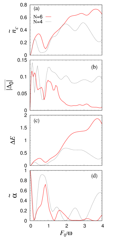
Figure 23: (a) $\widetilde{n_{c}}$, (b) $\overline{|\Delta_{0}|}$, (c) $\Delta E$, and (d) $\widetilde{\alpha}$ as functions of $F_{0}/\omega$ obtained by the ED method. We use $F(\tau)$ with the gaussian envelope. The parameters other than $F_{0}$ are the same as those in Fig. 22. In each panel, we show the results with $N=4$ by the dashed line for comparison, where $E_{1}-E_{0}=0.56$ and we use $\omega=0.6$.

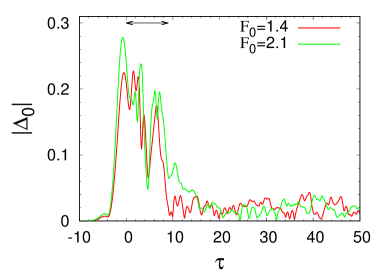
Figure 24: Time evolution of $|\Delta_{0}|$ for $F_{0}=1.4$ and $2.1$ obtained by the ED method. The other parameters are the same as those in Fig. 22. The double-headed arrow indicates the range $0<\tau<2\tau_{w}=2\pi/\omega$ of application of an electric field.

V.2.2 Excitations with continuous-wave laser

Next, we consider the case of CW excitations and examine time evolutions of physical quantities from the viewpoint of the Rabi oscillation. In Fig. 25, we show the time profiles of $n_{c}$ and $\alpha$ for different values of $F_{0}$ with $U^{\prime}=3.9>U^{\prime}_{\rm cr}$ for which the ground state before the photoexcitation is the BI. They exhibit an oscillation, the period of which becomes shorter with increasing $F_{0}$. For small $F_{0}$ ($F_{0}\lesssim 0.1$), the time profile of $n_{c}$ is well described by a single sinusoidal function of the form Eq. (24) as shown in Fig. 25(a), and the minimum value in the oscillation is close to the ground-state value of $n_{c}$ $(=0)$. Correspondingly, a nearly sinusoidal oscillation appears in $\alpha$. It is notable that we have $\alpha\sim 1$ when $n_{c}\sim 0$, whereas $\alpha\sim 0$ when $n_{c}$ exhibits its maximum. These behaviors are consistent with the Rabi oscillation as we have discussed in Sect. III. With increasing $F_{0}$, the oscillatory profiles in $n_{c}$ and $\alpha$ gradually become more complex. For $F_{0}\gtrsim 0.15$, a single sinusoidal function does not fit well to the data. Also, the minimum (maximum) in the oscillation of $n_{c}$ ($\alpha$) departs from its ground-state value, which is in contrast to the case with $F_{0}\lesssim 0.1$.

In Fig. 26(a), we show the Fourier transform of $n_{c}$ that is calculated from the data for $50\leq\tau\leq 400$. There is a sharp peak in each spectrum and its position that is denoted by $\Omega$ becomes larger for larger $F_{0}$. In Fig. 26(b), we plot the $F_{0}$ dependence of $\Omega$. For $F_{0}\lesssim 0.1$, $\Omega$ is nearly proportional to $F_{0}$: a function $\Omega=pF_{0}$ with $p=2.70$ fits well to the data. This result, in conjunction with the time profiles of $n_{c}$ and $\alpha$ shown in Fig. 25, indicates that for small $F_{0}$ the many-body dynamics under CW excitations is consistently interpreted from the viewpoint of the Rabi oscillation. At $F_{0}\sim 0.15$, $\Omega$ starts to deviate from the linear dependence on $F_{0}$. At this value of $F_{0}$, the appearance of complex oscillatory profiles in $n_{c}$ and $\alpha$ as well as the departure of these quantities from their ground-state values (Fig. 25) are observed. These properties are different from those in the atomic limit with the HF approximation where the linearity characterizing the Rabi oscillation basically appears for large $|F_{0}|$ as we have discussed in Sect. III A and Appendix A. The deviation of the ED results with $F_{0}\gtrsim 0.15$ from the relation $\Omega=pF_{0}$ that is expected in two-level systems may come from effects of photoexcited electrons away from the gap, which should be increasingly important with increasing $F_{0}$. We note, however, that some oscillatory behavior reminiscent of the Rabi oscillation appears even for $F_{0}>0.15$, especially within the first few cycles of the CW excitations (Fig. 25). Therefore, in the case of single cycle pulses we can expect that the $F_{0}/\omega$ dependences of physical quantities after the photoexcitation for $F_{0}>0.15$ are qualitatively understood with the help of the Rabi oscillation. In fact, Fig. 23 obtained with single cycle pulses indicates the signature of the Rabi oscillation for $F_{0}/\omega\lesssim 1$ ($F_{0}\lesssim 0.5$).

Finally, we examine the correspondence between the results with CW excitations and those with single cycle pulses in the same way as we have done in Sect. III A. We apply $\Omega_{R}^{\prime}=pF_{0}$ with $p=2.70$ to Eq. (24). For $\alpha$, we use Eq. (21) with $n^{G}_{c}=\Delta^{G}_{0}=0$. By setting $\tau=2\pi/\omega$ in these equations, we can deduce that $\widetilde{\alpha}$ ($\widetilde{n_{c}}$) for single cycle pulses exhibits a minimum (maximum) at $F_{0}/\omega\sim 0.19$ unless the constant $A$ in Eq. (24) strongly depends on $F_{0}$. For $\widetilde{\alpha}$, this value of $F_{0}/\omega$ is consistent with the results shown in Fig. 23, where it exhibits a minimum at $F_{0}/\omega=0.21$. For $\widetilde{n_{c}}$, its first maximum is located at $F_{0}/\omega=0.46$ which is larger than the above estimation. This discrepancy mainly comes from an increase in the amplitude of $n_{c}$ with increasing $F_{0}$ [Fig. 25(a)]: the $F_{0}$ dependence of $A$ is important in determining the maximum of $n_{c}$. This is in contrast to the time evolutions of $\alpha$ where it becomes almost zero in its first oscillation irrespective of the value of $F_{0}$ [Fig. 25(b)]. We note that this argument also holds for the case with the rectangular envelope where the maximum of $\widetilde{n_{c}}$ and the minimum of $\widetilde{\alpha}$ are located at $F_{0}/\omega=0.21$ and $0.32$, respectively, as shown in Appendix D.

Figure 25: Time evolutions of $n_{c}$ and $\alpha$ under CW excitations for different values of $F_{0}$ obtained by the ED method. We use $U=4$, $\mu_{C}=2.5$, $U^{\prime}=3.9$, and $\omega=0.7$. In (a), the dashed lines indicate the fitting results by a single sinusoidal function.

Figure 26: (a) Fourier transform of $n_{c}$. In each spectrum, the position of its largest peak is indicated by the arrow. The parameters are the same as those of Fig. 25. (b) Peak frequency $\Omega$ in Fourier transform of $n_{c}$ as a function of $F_{0}$. The solid line is a fitting result to the data with $F_{0}\leq 0.1$.

VI Discussion and Summary

Finally, we discuss possible experimental observation of photoinduced gap enhancement as well as the relevance of our results to Ta₂NiSe₅. Recent theoretical studies Seki_PRB14 ; Matsuura_JPSJ16 have shown that various equilibrium properties of Ta₂NiSe₅ such as the ARPES spectra Seki_PRB14 and the temperature dependence of magnetic susceptibility Salvo_JLCM86 can be reproduced by two- or three-orbital Hubbard models. Effects of the structural distortion observed at $T_{C}$ have been investigated using a three-orbital Hubbard model with e-ph interactions by the HF approximation Kaneko_PRB13 . It has been shown that the values of the e-ph interaction strengths needed to reproduce the experimentally observed distortion are one order of magnitude smaller than those of the transfer integrals and the e-e interaction strengths. Then, it has been argued that the EI in Ta₂NiSe₅ is ascribed to the BEC of electron-hole pairs which cooperatively induce the instability of the lattice distortion. These studies suggest that the photoinduced dynamics obtained in this paper based on the two-orbital Hubbard model [Eq. (1)] would be relevant to Ta₂NiSe₅.

In our mechanism, photoinduced gap enhancement occurs purely electronically when $\omega$ is comparable to the excitonic gap. Moreover, we have shown that e-ph couplings do not affect our results qualitatively. When $\omega$ is much larger than the excitonic gap, which is the case in recent experiments Mor_PRL17 , a theoretical study has shown that e-ph couplings are crucially important for the appearance of the gap enhancement Murakami_PRL17 . Thus, our mechanism is considered as an alternative route to this phenomenon.

In this paper, we consider the case where the upper and lower bands have the same bandwidth ($t_{c}=-t_{f}$). However, even when the two bandwidths are different Kaneko_PRB13 , we expect that the gap enhancement by the Rabi oscillation occurs as long as the initial system is a BEC-type EI or a nearby BI. This is because their dynamics should be basically understood from the real-space picture Tanaka_PRB18 where the analysis in the atomic limit presented in this paper is valid.

In order to examine the relevance of our results to experiments, we estimate the number of absorbed photons per site $n_{\rm ph}$. When $U=4$ and $U^{\prime}=3.3$ [Fig. 11(c)], we have $\Delta E=0.398$ for $|F_{0}|/\omega=0.44$ at which $\overline{|\Delta_{0}|}$ exhibits the first peak as a function of $|F_{0}|/\omega$. This corresponds to $n_{\rm ph}=\Delta E/\omega=0.32$. We note that a sizable gap enhancement appears with much smaller values of $n_{\rm ph}$. For instance, $15$% enhancement in $\overline{|\Delta_{0}|}$ is obtained for $|F_{0}|/\omega=0.2$ where we have $n_{\rm ph}=0.017$. In Ta₂NiSe₅, K. Okazaki et al. have reported that when the incident pump fluence is 1 ${\rm mJ}/{\rm cm}^{2}$, $n_{\rm ph}\sim 0.1$ per Ni atom whose $3d$ orbital hybridizes Se $4p$ orbital and forms a hole band Okazaki_NC18 . The threshold pump fluence for the appearance of the gap enhancement reported in Ref. 9 is $F_{C}=0.2$ ${\rm mJ}/{\rm cm}^{2}$, which may correspond to $n_{\rm ph}\sim 0.02$. This suggests that the pump fluence used in the current experimental studies is enough to observe the gap enhancement based on our mechanism unless $n_{\rm ph}$ depends largely on the value of the initial gap. However, at present a direct comparison between theoretical and experimental estimates is difficult by the following reasons. Firstly, in our model, we assume that the incident light induces the dipole transition whereas it does not affect the intraorbital electron motion. In order to realize this situation in real materials, the direction of light polarization as well as the crystal structure of the material are crucially important. For a material with a quasi-one dimensional structure like Ta₂NiSe₅, this indicates that the polarization of light should be perpendicular to the chain. The value of the matrix element for the dipole transition between the two bands is also important. Secondly, the pump-light frequency should be nearly tuned to the resonance condition. Note that in this case a recent theoretical study has shown that the gap enhancement does not appear when the incident light only affects the intraorbital electron motion Tanabe_PRB18 . Thirdly, the estimation of $n_{\rm ph}$ by the time-dependent HF method may be quantitatively inaccurate since it ignores the correlation effects Tanaka_JPSJ10 ; Miyashita_JPSJ10 . With regard to this point, from our ED results on small clusters with $U=4$ and $U^{\prime}=3.9$ where the ground state is the BI, we have $n_{\rm ph}=0.10$ for $F_{0}/\omega=0.1$ at which $\overline{|\Delta_{0}|}$ is maximally enhanced [Fig. 23]. This value of $n_{\rm ph}$ is comparable to the above-mentioned HF results.

We note that the gap enhancement with the help of the Rabi oscillation is irrespective of the dimensionality of the system. In fact, our results for one-dimensional systems are qualitatively unaltered even in the two-dimensional case Tanaka_PRB18 . Moreover, our ED results suggest that the Rabi-oscillation-assisted gap enhancement appears even when the effects of quantum fluctuations are considered, although how the dephasing and thermalization affect the dynamics remains as a future important problem.

In summary, we investigated dynamics of EIs induced by electric dipole transitions using the two-orbital Hubbard model. Through the HF analysis of the dynamics in the atomic limit, we have shown that the photoinduced gap enhancement in the EI for single cycle pulses reported previously Tanaka_PRB18 is explained in terms of the Rabi oscillation. The signature of the Rabi oscillation appears as a periodic behavior of physical quantities after the photoexcitation as functions of the dipole field strength $F_{0}$. We emphasize that although the Rabi oscillation is a one-site problem, it represents the essential feature of the photoinduced dynamics in the thermodynamic limit in the parameter range that we have considered in this paper. We have performed the ED calculations which strongly suggest the robustness of this phenomenon against the correlation effects and thus corroborate our HF results. The effects of the e-ph coupling have been examined within the HF approximation, indicating that they do not have a significant role on the gap enhancement in the present situation. Based on the present results and our previous work Tanaka_PRB18 , the condition for inducing the gap enhancement is summarized as follows: (i) The initial state is an EI in the BEC regime or a BI that is located near the EI. (ii) The pump-light frequency $\omega$ is near the initial gap. (iii) There is an optimal value of $F_{0}$ for enhancing the excitonic gap, which satisfies the relation $\Omega^{\prime}_{R}/\omega\sim 1/2$ with the Rabi frequency $\Omega^{\prime}_{R}\approx|F_{0}|$.

Appendix A Detailed dynamics in the atomic limit

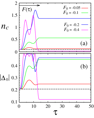
Figure 27: Time evolutions of (a) $n_{c}$ and (b) $|\Delta_{0}|$ for different values of $F_{0}$ with $U=1$, $\mu_{C}=0.5$, $U^{\prime}=0.45$, and $\omega=0.45$. The arrow indicates the range where $F(\tau)$ with the rectangular envelope is nonzero. The horizontal dashed line in each panel indicates the corresponding equilibrium value.

We show details of the real-time dynamics of mean-field order parameters in the atomic limit. We use $F(\tau)$ with the rectangular envelope [Eq. (4)]. The time profiles of $n_{c}$ and $\Delta_{0}$ for different values of $F_{0}$ are shown in Fig. 27 where the parameters are the same as those in Fig. 2. We introduce the psedospin operators as

$$\hat{S}_{\gamma}\equiv\Psi^{\dagger}\frac{1}{2}\sigma_{\gamma}\Psi,$$ (41)

where $\sigma_{\gamma}$ ($\gamma=x,y,z$) are the Pauli matrices and we omit the spin index in $\Psi_{\sigma}$ for brevity. With this representation, the expectation values of the pseudospin $S_{\gamma}=\langle\hat{S}_{\gamma}\rangle$ components are written as

$$S_{x}(\tau) ={\rm Re}\Delta_{0},$$ (A2a)

$$S_{y}(\tau) ={\rm Im}\Delta_{0},$$ (A2b)

$$S_{z}(\tau) =\frac{1}{4}(n_{c}-n_{f}),$$ (A2c)

which give $\Delta_{0}=S_{x}+iS_{y}$ and $n_{c}=2S_{z}+1$. By using the equation of motion for the pseudospin operators, the time evolution of ${\bm{S}}=(S_{x},S_{y},S_{z})$ is given by

$$\partial_{\tau}{\bm{S}}={\bm{B}}(\tau)\times{\bm{S}}(\tau),$$ (3)

where

$$B_{x} =2[U^{\prime}{\rm Re}\Delta_{0}-F(\tau)],$$ (A4a)

$$B_{y} =2U^{\prime}{\rm Im}\Delta_{0},$$ (A4b)

$$B_{z} =-(\epsilon^{c}-\epsilon^{f}).$$ (A4c)

In Figs. 28(a) and 28(b), we show the trajectory of $(S_{x},S_{y})$ and the time evolution of $\theta$ that has been defined in Eq. (33), respectively, for single cycle pulses with $F_{0}=-0.05$ and $-0.2$. We use $\mu_{C}=0.5$, $U^{\prime}=0.45$, and $\omega=0.45$. For $F_{0}=-0.05$, $|\Delta_{0}|$ ($=\sqrt{{S_{x}}^{2}+{S_{y}}^{2}}$) is slightly increased by the photoexcitation, whereas it is largely enhanced for $F_{0}=-0.2$. After the photoexcitation, the value of $|\Delta_{0}|$ is conserved and $\theta$ rotates with almost a constant velocity. As we increase $|F_{0}|$, the velocity becomes larger as shown in Fig. 28(b).

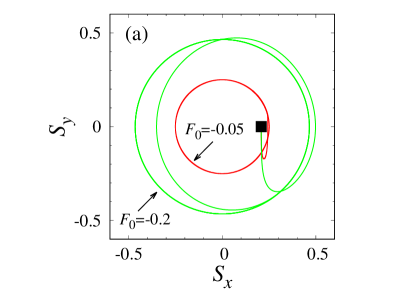
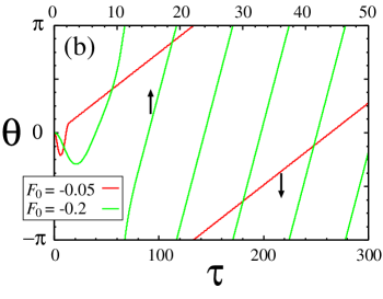
Figure 28: (a) Trajectory of ($S_{x},S_{y}$) and (b) time evolution of $\theta$ for $F_{0}=-0.05$ and $-0.2$ with rectangular envelope of Eq. (4). We use $U=1$, $\mu_{C}=0.5$, $U^{\prime}=0.45$ and $\omega=0.45$. For $F_{0}=-0.05$ ($F_{0}=-0.2$), we show the time domain $0\leq\tau\leq 300$ ($0\leq\tau\leq 50$). In (a), the solid square indicates the initial position of ($S_{x},S_{y}$).

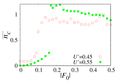
Figure 29: $\overline{n_{c}}$ as a function of $|F_{0}|$ with $U^{\prime}=0.45$ and $0.55$ for the case of CW excitations. We use $\mu_{C}=0.5$ and $\omega=0.45$ ($\omega=0.6$) for $U^{\prime}=0.45$ ($U^{\prime}=0.55$).

Next, we discuss results under CW excitations. As we have shown in Fig. 6, $n_{c}$ oscillates near its ground-state value for small $|F_{0}|$ ($F_{0}=-0.05$), whereas it exhibits a large oscillation for large $|F_{0}|$ ($F_{0}\lesssim-0.1$). Figure 29 shows $\overline{n_{c}}$ ($=2\overline{S_{z}}+1$) as a function of $|F_{0}|$ for $U^{\prime}=0.45$ and $0.55$. For both cases, there is a threshold $F^{c}_{0}$ at which $\overline{n_{c}}$ abruptly increases. We obtain $F^{c}_{0}=-0.1$ for $U^{\prime}=0.45$ and $F^{c}_{0}=-0.16$ for $U^{\prime}=0.55$. Such a dynamical transition has been previously reported in one-dimensional excitonic insulators within the HF theory Murakami_PRL17 .

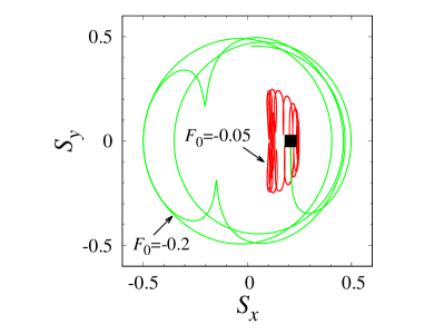
Figure 30: Trajectory of ($S_{x},S_{y}$) under CW excitations for $F_{0}=-0.05$ and $-0.2$. We use $U^{\prime}=0.45$ and $\omega=0.45$. For $F_{0}=-0.05$ ($F_{0}=-0.2$), we show the time domain $0\leq\tau\leq 300$ ($0\leq\tau\leq 50$). The open square indicates the initial point of ($S_{x},S_{y}$).

In the following, we examine the difference between the dynamics for $|F_{0}|<|F^{c}_{0}|$ and that for $|F_{0}|>|F^{c}_{0}|$. First, we consider the case of $U^{\prime}=0.45$ where the initial state is in the EP. We show the trajectory of ($S_{x},S_{y}$) with $F_{0}=-0.05$ ($|F_{0}|<|F^{c}_{0}|$) and $-0.2$ ($|F_{0}|>|F^{c}_{0}|$) under CW excitations with $\omega=0.45$ in Fig. 30. For $F_{0}=-0.05$, ($S_{x},S_{y}$) is bound near the ground-state position, whereas it is unbound for $F_{0}=-0.2$. This corresponds to bound and unbound oscillations in $n_{c}$ for $F_{0}=-0.05$ and $-0.2$ (Fig. 6), respectively. In Fig. 31(a), we show the Fourier transform of $n_{c}$ for small $|F_{0}|$ ($<|F^{c}_{0}|$), indicating that $n_{c}$ has one slow oscillation component with frequency $\Omega^{S}\lesssim 0.15$ and two fast components with frequencies $\Omega^{f\pm}$ near $\omega$, which we can write as $\Omega^{f\pm}=\omega\pm\delta\Omega$. Both $\Omega^{S}$ and $\delta\Omega$ increase with increasing $|F_{0}|$. When $|F_{0}|$ is small ($|F_{0}|<0.06$), the peak at $\Omega^{S}$ is dominant, whereas those at $\Omega^{f\pm}$ become dominant for $0.06<|F_{0}|<|F^{c}_{0}|$. As we increase $|F_{0}|$ further ($|F_{0}|>|F^{c}_{0}|$), the spectra change drastically as we have shown in Fig. 7. In Fig. 31(b), we show the $|F_{0}|$ dependence of $\Omega^{S}$. When $|F_{0}|\lesssim 0.06$, $\Omega^{S}$ is proportional to $|F_{0}|$ and we have $\Omega^{S}=p|F_{0}|$ with $p=0.63$ that is different from the value ($p=1.24$) obtained in Sect. III A for $|F_{0}|>|F^{c}_{0}|$. The region of $|F_{0}|$ ($0.06<|F_{0}|<|F^{c}_{0}|$) where the value of $p$ largely deviates coincides with that where $\overline{n_{c}}$ exhibits the abrupt increase in Fig. 29. These results indicate that the dynamics for $|F_{0}|<|F^{c}_{0}|$ have a character different from that for $|F_{0}|>|F^{c}_{0}|$.

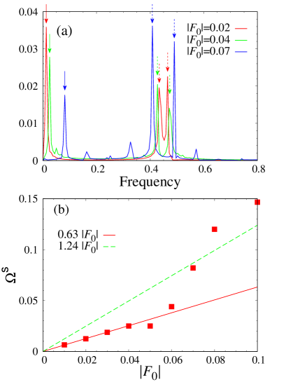
Figure 31: (a) Fourier transform of $n_{c}$ for $|F_{0}|<|F^{c}_{0}|$ with $U^{\prime}=0.45$ and $\omega=0.45$. The peaks corresponding to $\Omega^{S}$ ($\Omega^{\pm f}$) are indicated by the solid (dashed) arrows. (b) $|F_{0}|$ dependence of $\Omega^{S}$. The solid line is fit to the data with $|F_{0}|\leq 0.06$. The fitting result in Fig. 8 for $U^{\prime}=0.45$ is also shown by the dashed line.

Next, we show results with $U^{\prime}=0.55$ where the initial state is in the DP. The trajectory of ($S_{x},S_{y}$) for $F_{0}=-0.05$ ($|F_{0}|<|F^{c}_{0}|$) and $F_{0}=-0.25$ ($|F_{0}|>|F^{c}_{0}|$) with $\omega=0.6$ is depicted in Fig. 32. Similar to the case of $U^{\prime}=0.45$, $(S_{x},S_{y})$ is bound near its initial position for $|F_{0}|<|F^{c}_{0}|$, whereas it is unbound for $|F_{0}|>|F^{c}_{0}|$. In Fig. 33(a), we show the Fourier transform of $n_{c}$ for $|F_{0}|<|F^{c}_{0}|$. The dominant oscillation components in $n_{c}$ have frequencies $\Omega^{f\pm}=\omega\pm\delta\Omega$, and there is a slow oscillation component with $\Omega^{S}=2\delta\Omega$ whose amplitude is higher order in $|F_{0}|$. When $|F_{0}|$ is small, we can solve Eq. (3) in the lowest order of $F_{0}$ with the initial condition ${\bm{S}}(\tau=0)=(0,0,-1/2)$ as

$$S^{x}(\tau) =\frac{F_{0}}{\omega^{2}-a^{2}}(a\sin\omega\tau-\omega\sin a\tau),$$ (A5a)

$$S^{y}(\tau) =\frac{\omega F_{0}}{\omega^{2}-a^{2}}(\cos a\tau-\cos\omega\tau),$$ (A5b)

$$S^{z}(\tau) =\frac{\omega F_{0}}{\omega^{2}-a^{2}}\Bigl{[}\frac{1-\cos(\omega+a)\tau}{\omega+a}$$

$$+\frac{1-\cos(\omega-a)\tau}{\omega-a}+\frac{1-\cos 2\omega\tau}{2\omega}\Bigr{]},$$ (A5c)

where $a=\mu_{C}-U+U^{\prime}$. From Eq. (A5c), we find that for $|F_{0}|\rightarrow 0$, $\delta\Omega\rightarrow a=0.05$ and there is an oscillation component with frequency $2\omega=1.2$, which are consistent with the numerical results shown in Fig. 33(a). As we increase $|F_{0}|$, $\Omega^{S}$ increases. $\Omega^{S}=0.1+10|F_{0}|^{2}$ is fit well to the data as shown in Fig. 33(b). These results indicate that the dynamics for $|F_{0}|<|F^{c}_{0}|$ is essentially different from that for $|F_{0}|>|F^{c}_{0}|$ as in the case of $U^{\prime}=0.45$. In fact, the spectra of $n_{c}$ for $|F_{0}|>|F^{c}_{0}|$ (not shown) are largely different from those for $|F_{0}|<|F^{c}_{0}|$.

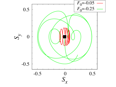
Figure 32: Similar plot as Fig. 30 for $U^{\prime}=0.55$ and $\omega=0.6$. We show the time domain of $0\leq\tau\leq 150$ ($0\leq\tau\leq 50$) for $F_{0}=-0.05$ ($F_{0}=-0.2$).

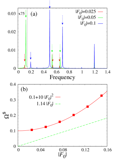
Figure 33: (a) Fourier transform of $n_{c}$ for $|F_{0}|<|F^{c}_{0}|$ with $U^{\prime}=0.55$ and $\omega=0.6$. The peaks corresponding to $\Omega^{S}$ ($\Omega^{\pm f}$) are indicated by the solid (dashed) arrows. (b) $|F_{0}|$ dependence of $\Omega^{S}$. The solid curve indicates the fitting result. The fitting result in Fig. 8 for $U^{\prime}=0.55$ is also shown by the dashed line.

Appendix B Effects of $\tau$-dependence of $n_{c}$ and $\Delta_{0}$ in Eq. (14) on the dynamics

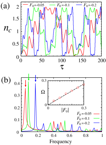
Figure 34: (a) Time profile of $n_{c}$ under CW excitations obtained by the time evolution operator in which we artificially replace $n_{c}$ and $\Delta_{0}$ by those at $\tau=0$. (b) Fourier transform of (a). In each spectrum, the position of the largest peak, $\Omega$, is indicated by the arrow. In the inset, the $|F_{0}|$ dependence of $\Omega$ is shown, where the fitting result is also depicted by the dashed line.

As we have mentioned in III A 3, Eq. (14) possesses $\tau$-dependent mean-field order parameters from which the time evolution operator is constructed. In order to examine how their $\tau$-dependence affects the dynamics in the atomic limit, we artificially replace $n_{c}$ and $\Delta_{0}$ in the time evolution operator by $n^{G}_{c}$ and $\Delta^{G}_{0}$, respectively, and compute the time profile of $n_{c}$ under CW excitations. The parameters we used are the same as those in Fig. 6. The results are shown in Fig. 34(a). Compared with Fig. 6, a large oscillation in $n_{c}$ appears even when $|F_{0}|$ is small. From the Fourier spectra shown in Fig. 34(b), we obtain $\Omega\sim p|F_{0}|$ with $p=0.86$. This result indicates that the $\tau$ dependence of the order parameters is important in determining the dynamics for small $|F_{0}|$ ($|F_{0}|<0.1$). However, it does not alter the dynamics qualitatively for larger $|F_{0}|$ where the Rabi oscillation appears in Fig. 6. These facts give a reason why the quantitative difference between the value of $\widetilde{n_{c}}$ for single cycle pulses and that of $n_{c}$ at $\tau=2\pi/\omega$ computed from Eq. (24) becomes large for small $|F_{0}|$ ($|F_{0}|/\omega\lesssim 0.3$), which can be seen in Fig. 9.

Appendix C HF results in the presence of phonons for the case of rectangular-envelope pulse

We show the $|F_{0}|/\omega$ dependence of $\overline{n_{c}}$ in the presence of the e-ph coupling when we use $F(\tau)$ with the rectangular envelope. In Fig. 35, the results in the atomic limit are depicted. The parameters are the same as those in Fig. 17.

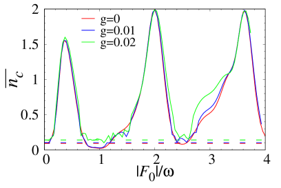
Figure 35: Same plot as Fig. 17 except that we use $F(\tau)$ with the rectangular envelope.

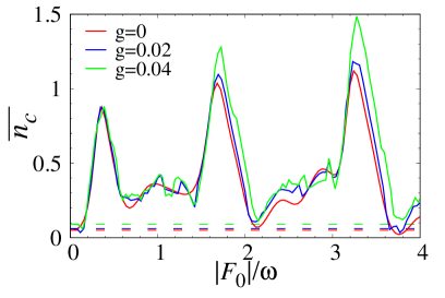
Figure 36: Same plot as Fig. 19 except that we use $F(\tau)$ with the rectangular envelope.

For the one-dimensional model with $t_{f}=1$ and $t_{c}=-1$, the results are shown in Fig. 36 where the parameters are the same as those in Fig. 19. From Figs. 35 and 36, we confirm that the e-ph coupling has little effects on the $|F_{0}|/\omega$ dependence of $\overline{n_{c}}$ as in the case of the gaussian-envelope pulse shown in Figs. 17 and 19.

Appendix D ED results for the case of rectangular-envelope pulse

In Fig. 37, we show $\widetilde{n_{c}}$, $\overline{|\Delta_{0}|}$, $\Delta E$, and $\widetilde{\alpha}$ as functions of $F_{0}/\omega$ obtained by the ED method when we use $F(\tau)$ with the rectangular envelope. The parameters are the same as those in Fig. 23. For $F_{0}/\omega\lesssim 1$, the $F_{0}/\omega$ dependence of these quantities is similar to those in Fig. 23, indicating that the pulse shape does not significantly affect our results as in the case of the HF method. The cyclic behavior is evident even for $F_{0}/\omega>1$, although in this region the increase (decrease) in $\widetilde{n_{c}}$ and $\Delta E$ ($\widetilde{\alpha}$) does not correspond to the large enhancement in $\overline{|\Delta_{0}|}$, which is in contrast to the results with the HF method shown in Fig. 13. This is caused by the dephasing discussed in Sect. V, which suppresses $|\Delta_{0}|$. In fact, for $F_{0}/\omega\sim 1.6$ and $3.2$ of the results with $N=6$, where $\widetilde{n_{c}}$ and $\Delta E$ exhibit a peak and $\widetilde{\alpha}\sim 0$, we have confirmed that the time profile of $|\Delta_{0}|$ is similar to that in Fig. 24.

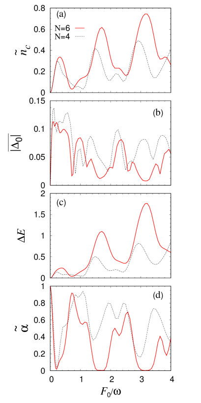
Figure 37: Same plots as Fig. 23 by the ED method except that we use $F(\tau)$ with the rectangular envelope.

- (1) K. Onda, S. Ogihara, K. Yonemitsu, N. Maeshima, T. Ishikawa, Y. Okimoto, X. Shao, Y. Nakano, H. Yamochi, G. Saito, and S. Koshihara, Phys. Rev. Lett. 101, 067403 (2008).
- (2) D. Fausti, R. I. Tobey, N. Dean, S. Kaiser, A. Dienst, M. C. Hoffmann, S. Pyon, T. Takayama, H. Takagi, and A. Cavalleri, Science 331, 189 (2011).
- (3) T. Ishikawa, Y. Sagae, Y. Naitoh, Y. Kawakami, H. Itoh, K. Yamamoto, K. Yakushi, H. Kishida, T. Sasaki, S. Ishihara, Y. Tanaka, K. Yonemitsu, and S. Iwai, Nat. Commun. 5, 5528 (2014).
- (4) W. Hu, S. Kaiser, D. Nicoletti, C. R. Hunt, I. Gierz, M. C. Hoffmann, M. Le Tacon, T. Loew, B. Keimer, A. Cavalleri, Nat. Mater. 13, 705 (2014).
- (5) S. Kaiser, C. R. Hunt, D. Nicoletti, W. Hu, I. Gierz, H. Y. Liu, M. Le Tacon, T. Loew, D. Haug, B. Keimer, A. Cavalleri, Phys. Rev. B 89, 184516 (2014).
- (6) L. Stojchevska, I. Vaskivskyi, T. Mertelj, P. Kusar, D. Svetin, S. Brazovskii, and D. Mihailovic, Science 344, 177 (2014).
- (7) M. Mitrano, A. Cantaluppi, D. Nicoletti, S. Kaiser, A. Perucchi, S. Lupi, P. Di Pietro, D. Pontiroli, M. Riccò, S. R. Clark, D. Jaksch, A. Cavalleri, Nature 530, 461 (2016).
- (8) A. Singer, S. K. K. Patel, R. Kukreja, V. Uhl, J. Wingert, S. Festersen, D. Zhu, J. M. Glownia, H. T. Lemke, S. Nelson, M. Kozina, K. Rossnagel, M. Bauer, B. M. Murphy, O. M. Magnussen, E. E. Fullerton, and O. G. Shpyrko, Phys. Rev. Lett. 117, 056401 (2016).
- (9) S. Mor, M. Herzog, D. Golez, P. Werner, M. Eckstein, N. Katayama, M. Nohara, H. Takagi, T. Mizokawa, C. Monney, and J. Stahler, Phys. Rev. Lett. 119, 086401 (2017).
- (10) Y. Kawakami, Y. Yoneyama, T. Amano, H. Itoh, K. Yamamoto, Y. Nakamura, H. Kishida, T. Sasaki, S. Ishihara, Y. Tanaka, K. Yonemitsu, and S. Iwai, Phys. Rev. B 95, 201105(R) (2017).
- (11) H. T. Lu, S. Sota, H. Matsueda, J. Bonca, and T. Tohyama, Phys. Rev. Lett. 109, 197401 (2012).
- (12) N. Tsuji, T. Oka, H. Aoki, and P. Werner, Phys. Rev. B 85, 155124 (2012).
- (13) H. Hashimoto, H. Matsueda, H. Seo, and S. Ishihara, J. Phys. Soc. Jpn. 83, 123703 (2014).
- (14) H. Hashimoto, H. Matsueda, H. Seo, and S. Ishihara, J. Phys. Soc. Jpn. 84, 113702 (2015).
- (15) H. Yanagiya, Y. Tanaka, and K. Yonemitsu, J. Phys. Soc. Jpn. 84, 094705 (2015).
- (16) M. Nakagawa and N. Kawakami, Phys. Rev. Lett. 115, 165303 (2015).
- (17) K. Yonemitsu, J. Phys. Soc. Jpn. 86, 024711 (2017).
- (18) K. Ido, T. Ohgoe, and M. Imada, Sci. Adv. 3, e1700718 (2017).
- (19) Y. Murakami, D. Gole, M. Eckstein, P. Werner, Phys. Rev. Lett. 119, 247601 (2017).
- (20) K. Oya and A. Takahashi, Phys. Rev. B 97, 115147 (2018).
- (21) Y. Tanaka, M. Daira, and K. Yonemitsu, Phys. Rev. B 97, 115105 (2018).
- (22) T. Tanabe, K. Sugimoto, and Y. Ohta, Phys. Rev. B 98, 235127 (2018).
- (23) N. F. Mott, Phil. Mag. 6, 287 (1961).
- (24) R. S. Knox, Solid State Phys. Suppl. 5, 100 (1963).
- (25) D. Jerome, T. M. Rice, and W. Kohn, Phys. Rev. 158, 462 (1967).
- (26) B. I. Halperin and T. M. Rice, Rev. Mod. Phys. 40, 755 (1968).
- (27) J. Kunes, J. Phys.: Cond. Mat. 27, 333201 (2015).
- (28) Y. Wakisaka, T. Sudayama, K. Takubo, T. Mizokawa, M. Arita, H. Namatame, M. Taniguchi, N. Katayama, M. Nohara, and H. Takagi, Phys. Rev. Lett. 103, 026402 (2009).
- (29) F. J. Di Salvo, C. H. Chen, R. M. Fleming, J. V. Waszczak, R. G. Dunn, S. A. Sunshine, James A. Ibers, J. Less-Common Met. 116, 51 (1986).
- (30) Y. F. Lu, H. Kono, T. I. Larkin, A. W. Rost, T. Takayama, A, V. Boris, B. Keimer, and H. Takagi, Nat. Commun. 8, 14408 (2017).
- (31) S. Li, S. Kawai, Y. Kobayashi, and M. Itoh, Phys. Rev. B 97, 165127 (2018).
- (32) K. Seki, Y. Wakisaka, T. Kaneko, T. Toriyama, T. Konishi, T. Sudayama, N. L. Saini, M. Arita, H. Namatame, M. Taniguchi, N. Katayama, M. Nohara, H. Takagi, T. Mizokawa, and Y. Ohta, Phys. Rev. B 90, 155116 (2014).
- (33) K. Sugimoto and Y. Ohta, Phys. Rev. B 94, 085111 (2016).
- (34) H. Matsuura and M. Ogata, J. Phys. Soc. Jpn. 85, 093701 (2016).
- (35) K. Sugimoto, S. Nishimoto, T. Kaneko, and Y. Ohta, Phys. Rev. Lett. 120, 247602 (2018).
- (36) D. Gole, P. Werner, and M. Eckstein, Phys. Rev. B 94, 035121 (2016).
- (37) The assumption that and are independent of is in fact validated by performing unrestricted HF calculations in real space that can treat inhomogeneous mean-field solutions.
- (38) A. Terai and Y. Ono, Prog. Theor. Phys. Suppl. 113, 177 (1993).
- (39) M. Kuwabara and Y. Ono, J. Phys. Soc. Jpn. 64, 2106 (1995).
- (40) Y. Tanaka and K. Yonemitsu, J. Phys. Soc. Jpn. 79, 024712 (2010).
- (41) If the initial order parameters are independent of , the expectation values like and with are always zero during the mean-field dynamics. This can be verified by using the equations of motion for these expectation values under the Hamiltonian Eq. (8). Therefore, and are independent of at any .
- (42) T. Kaneko, K. Seki, and Y. Ohta, Phys. Rev. B 85, 165135 (2012).
- (43) B. Zocher, C. Timm, and P. M. R. Brydon, Phys. Rev. B 84, 144425 (2011).
- (44) V.-N. Phan, K. W. Becker, and H. Fehske, Phys. Rev. B 81, 205117 (2010).
- (45) K. Seki, R. Eder, and Y. Ohta, Phys. Rev. B 84, 245106 (2011).
- (46) I. I. Rabi, Phys. Rev. 51, 652 (1937).
- (47) L. Allen and J. H. Eberly, Optical Resonance and Two-Level Atoms (Dover Publications, New York, 1987).
- (48) A. Ono, H. Hashimoto, and S. Ishihara, Phys. Rev. B 94, 115152 (2016).
- (49) K. Nishioka and K. Yonemitsu, J. Phys. Soc. Jpn. 83, 024706 (2014).
- (50) T. Kaneko, T. Toriyama, T. Konishi, and Y. Ohta, Phys. Rev. B 87, 035121 (2013).
- (51) K. Okazaki, Y. Ogawa, T. Suzuki, T. Yamamoto, T. Someya, S. Michimae, M. Watanabe, Y. Lu, M. Nohara, H. Takagi, N. Katayama, H. Sawa, M. Fujisawa, T. Kanai, N. Ishii, J. Itatani, T. Mizokawa, S. Shin, Nat. Commun. 9, 4322 (2018).
- (52) S. Miyashita, Y. Tanaka, S. Iwai, and K. Yonemitsu, J. Phys. Soc. Jpn. 79, 034708 (2010).
- (53) H. Watanabe, K. Seki, and S. Yunoki, J. Phys.: Conf. Ser. 592, 012097 (2015).