Single Image Cloud Detection via Multi-Image Fusion

Abstract

Artifacts in imagery captured by remote sensing, such as clouds, snow, and shadows, present challenges for various tasks, including semantic segmentation and object detection. A primary challenge in developing algorithms for identifying such artifacts is the cost of collecting annotated training data. In this work, we explore how recent advances in multi-image fusion can be leveraged to bootstrap single image cloud detection. We demonstrate that a network optimized to estimate image quality also implicitly learns to detect clouds. To support the training and evaluation of our approach, we collect a large dataset of Sentinel-2 images along with a per-pixel semantic labelling for land cover. Through various experiments, we demonstrate that our method reduces the need for annotated training data and improves cloud detection performance.

Index Terms—  weakly-supervised learning, multi-image fusion, segmentation, clouds

1 Introduction

As overhead imagery captured via remote sensing becomes more abundant, it is increasingly relied upon as an important source of information for understanding locations and how they change over time. For example, methods have been proposed for extracting roads [1], detecting buildings [2], estimating land cover [3], and interpreting the effects of natural disasters [4]. Unfortunately, various artifacts contained in the captured imagery, such as clouds, snow, and shadows, negatively impact the performance of these methods.

Clouds and their properties have long been researched due to their impact on weather and climate processes [5]. In an empirical study Wylie et al. [6] analyze cloud cover over a 22 year period using atmospheric sounding, finding that approximately 75 percent off all observations indicated clouds. Given their high frequency, clouds present persistent challenges for interpreting overhead imagery and many methods have been proposed for identifying them [7, 8].

The primary challenge is that the appearance of clouds can vary dramatically and collecting manually annotated data is time consuming and expensive. This issue is further compounded by the various sensor types and resolutions of satellite imagery, as well as differences in locations around the globe. Consider the scenario of transitioning to a new sensor. Instead of collecting large amounts of new annotations, a method is needed that can function with minimal supervision. In this work we explore how recent advances in multi-image fusion can be extended to support cloud detection.

First, we design an architecture for weakly-supervised multi-image fusion that learns to estimate image quality. Then, we describe two approaches which take advantage of the resulting quality network to produce a cloud detector. To support the training and evaluation of our methods, we collect a large dataset of overhead images captured at varying timesteps and varying levels of cloud cover. Our contributions include: 1) an analysis of multi-image fusion on real data, 2) two approaches for identifying clouds that require limited supervision, and 3) an extensive evaluation, achieving state-of-the-art results on a benchmark dataset.

2 Approach

Our approach for identifying clouds uses multi-image fusion as a form of bootstrapping, reducing the need for annotated training data. We start by describing the architecture for multi-image fusion and then describe how we extend this architecture for detecting clouds.

2.1 Multi-Image Fusion

We apply multi-image fusion to take a stack of images over the same region, $I=\{I_{1},\ldots,I_{K}\}$, where $I_{j}\in R^{h\times w\times 3}$, and produce a fused image, $F=\phi(I)$, such that $F$ is free of artifacts. Our approach is inspired by the recent work of Rafique et al. [9]. There are two main steps: 1) estimating a per-pixel quality mask for each image then using the qualities to compute a fused image and 2) passing the fused image through a segmentation network to produce a per-pixel semantic labeling. When trained end-to-end, this architecture learns to estimate per-pixel image qualities that can be used to produce a fused image with reduced artifacts, without requiring explicit labels.

2.1.1 Dataset

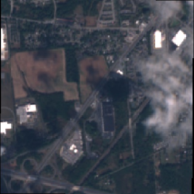
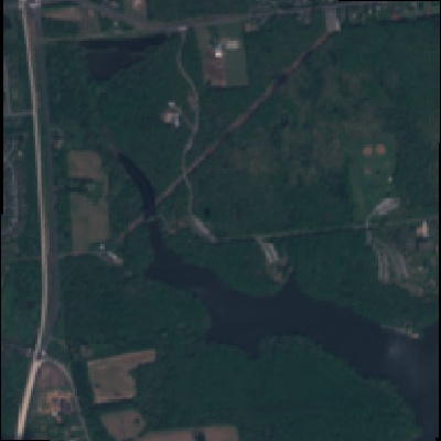
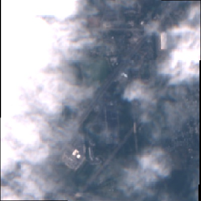
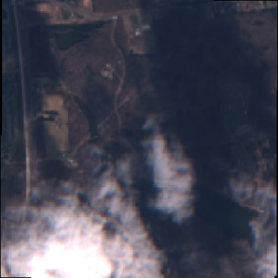
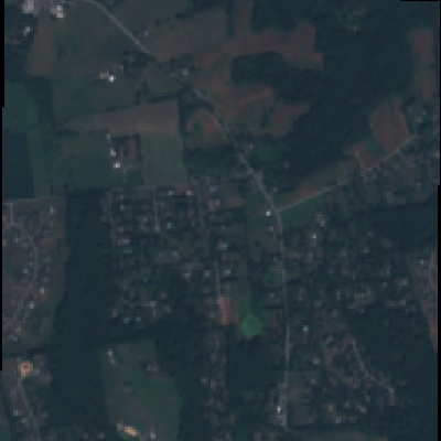
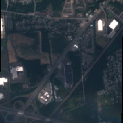
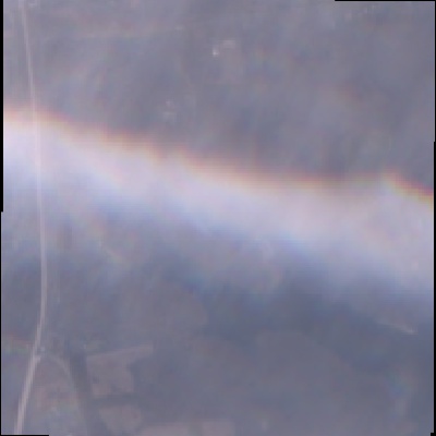
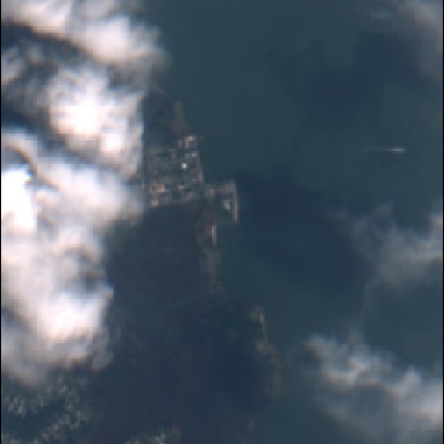
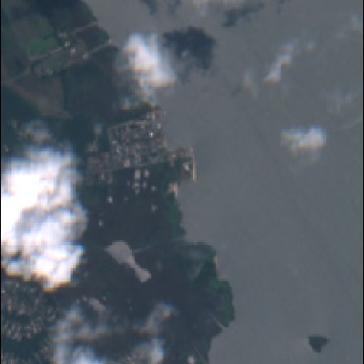
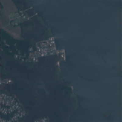
To support the training of our methods, we collected Sentinel-2 imagery from the state of Delaware with varying levels of cloud cover. Starting from a bounding box around the state, we generated a set of non-overlapping tiles using the standard XYZ style spherical Mercator tile. For each tile, we collected a semantic labeling from the Chesapeake Land Cover dataset [3], removing tiles without valid labels. For each remaining tile, we randomly downloaded six Sentinel-2 images (RGB bands) from the year 2019 that satisfied the constraint of having between 10% and 50% cloud cover in the parent Sentinel-2 image strip. This process resulted in $1033$ unique locations and $6198$ images (of size $512\times 512$). Figure 1 shows some example images from our dataset.

2.1.2 Method

Each image $I_{j}$ is first passed through a quality network which outputs a per-pixel quality mask $Q_{j}\in R^{h\times w}$ for each pixel $p$, such that $Q_{j}(I_{j}(p))\in[0,1]$. Given quality masks for each image, a relative quality score at each pixel is computed by applying a softmax across images:

$$Q^{*}_{j}(p)=\frac{e^{Q_{j}(p)}}{\sum_{k=1}^{K}e^{Q_{k}(p)}}.$$ (1)

The final fused image $F_{j}$ is obtained by averaging the images weighted by the relative quality score:

$$F_{j}(p)=\sum_{j=1}^{K}I_{j}(p)Q^{*}_{j}(p).$$ (2)

The fused image $F_{j}$ is passed through a segmentation network to produce a per-pixel labeling. The entire architecture, both quality network and segmentation network, are optimized using a cross-entropy loss function.

2.1.3 Architecture Details

For the quality network, we use a slightly modified U-Net [10] with the same number of layers but a quarter of the feature maps compared to the original work. The final activation is a sigmoid. For the segmentation network, we build on LinkNet [11], a modern, lightweight segmentation architecture that follows an encoder/decoder approach. Specifically, we use LinkNet-34, which is LinkNet with a ResNet-34 [12] encoder. We initialize the encoder with weights from a network pretrained on ImageNet.

2.2 Detecting Clouds

Fig. 1: Examples from our dataset for multi-image fusion. (top) Land cover labeling from the Chesapeake Land Cover dataset [3]. (bottom) Images of the same location with varying cloud cover.

Image (1 of 6)	Quality	Image (2 of 6)	Quality	Fused	Target	Prediction

Fig. 2: Qualitative examples of multi-image fusion. (left) Example images and estimated quality masks. (right) The fused image produced using the relative quality scores, the target segmentation mask, and our prediction.

The quality network learns to identify artifacts in the training data that negatively impact the final segmentation, for example clouds and regions of no data. We describe two approaches which use the quality network, trained for multi-image fusion, as a starting point for learning a cloud detector (per-pixel binary classification). For these methods, we use the dataset recently introduced by Liu et al. [13] with 100 training images and 20 testing images.

2.2.1 Quality Calibration

We apply Platt scaling (which we refer to as quality calibration) to transform the outputs of the quality network into a distribution over classes (cloud/not cloud). In practice, this means we fit a logistic regression model:

$$P(y=1|Q_{j}(p))=\frac{1}{1+e^{\beta_{0}Q_{j}(p)+\beta_{1}}},$$ (3)

where $\beta_{0}$ and $\beta_{1}$ are two learned parameters.

2.2.2 Fine-Tuning the Quality Network

Alternatively, we employ transfer learning, freezing all layers of the quality network except the final three convolutional layers (the last upsampling block and the final $1\times 1$ convolution). Then, we fine-tune the network for cloud detection. We optimize the network using the following loss function:

$$\mathcal{L}=\mathcal{L}_{bce}+(1-\mathcal{L}_{dice})$$ (4)

where $\mathcal{L}_{bce}$ is binary cross entropy, a standard loss function used in binary classification tasks, and $\mathcal{L}_{dice}$ is the dice coefficient, which measures spatial overlap.

2.3 Implementation Details

Our methods are implemented using the PyTorch [14] framework and optimized using RAdam [15] with Lookahead [16] ($k=5,\alpha=.5$). The learning rate is $\lambda=10^{-4}$ ($10^{-2}$ when fine-tuning). We train all networks with a batch size of 10 for 100 epochs and train on random crops of size $416\times 416$. For multi-image fusion, we randomly sample 4 images per location during training.

3 Evaluation

We evaluate our methods both qualitatively and quantitatively through a variety of experiments.

3.1 Visual Analysis of Multi-Image Fusion on Real Data

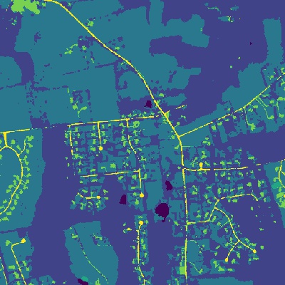
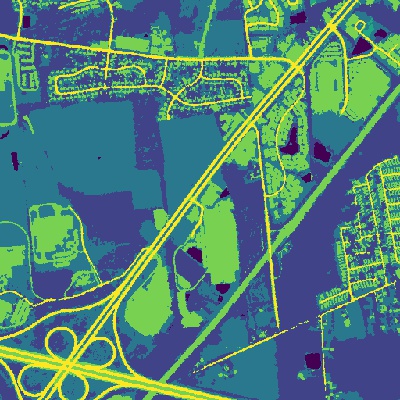
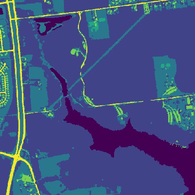
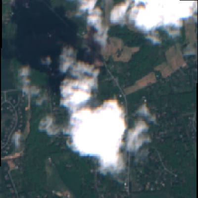
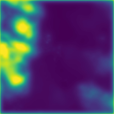
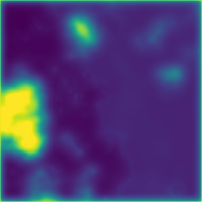
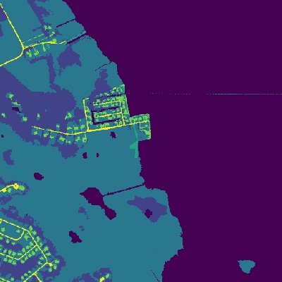
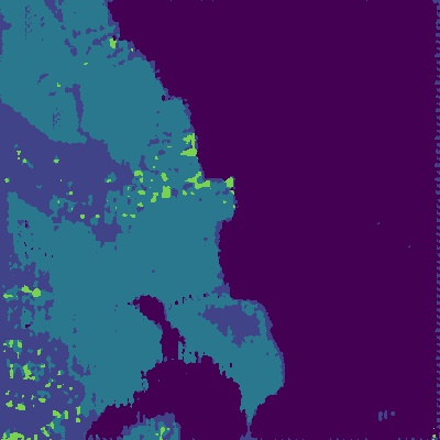
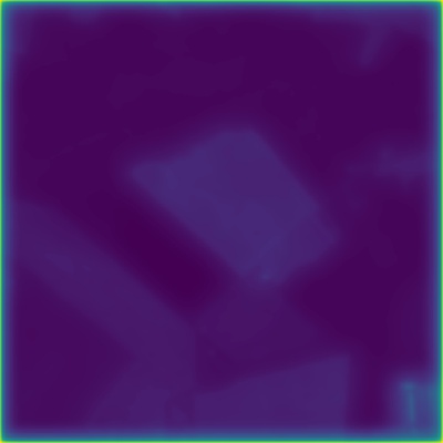
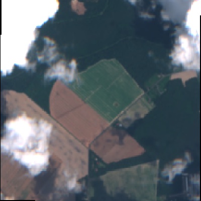
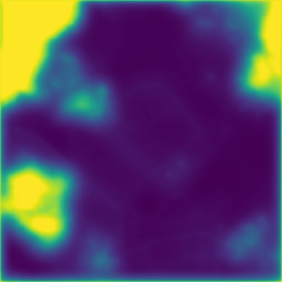
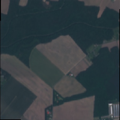
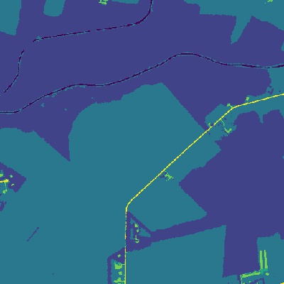
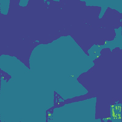
Previous work on multi-image fusion used training data augmented with synthetic clouds [9]. In our work, we train and evaluate our approach using real images with varying levels of cloud cover. Figure 2 shows example output from our network (described in Section 2.1), including: example images alongside the estimated quality mask, the fused image using the relative quality scores, the target label from the Chesapeake Land Cover dataset [3], and our prediction. The estimated quality masks clearly identify artifacts in the imagery, such as clouds.

3.2 Quantitative Analysis of Cloud Detection

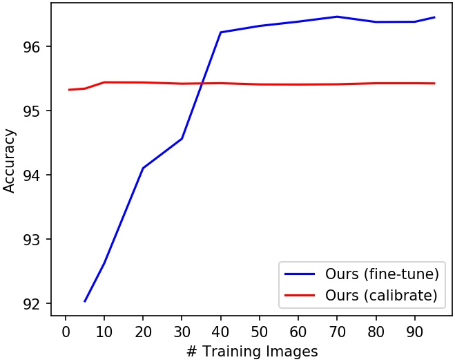
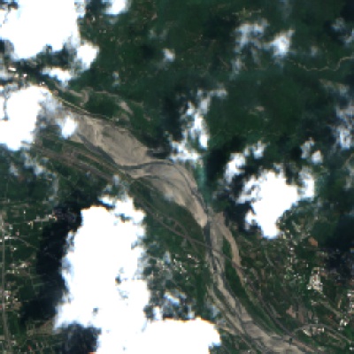
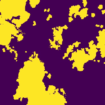
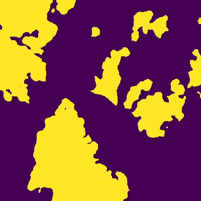
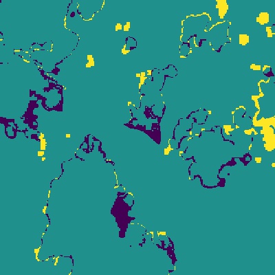
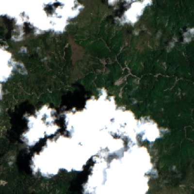
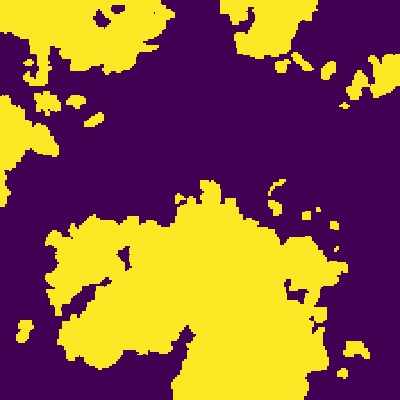
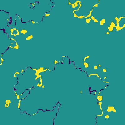
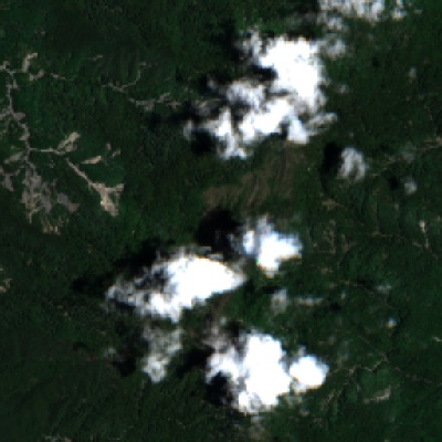
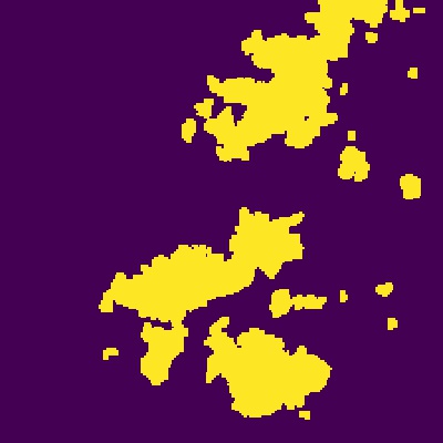
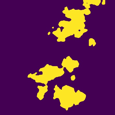
Using the dataset recently introduced by Liu et al. [13], we quantitatively evaluate our methods ability to detect clouds. Table 1 shows the results of this experiment. We compare against a baseline, Ours (threshold), that naïvely thresholds the quality masks at $.5$ (treating anything below the threshold as a cloud). The baseline, which requires no direct supervision, is able to correctly classify over 91% of pixels. Applying quality calibration, Ours (calibrate), to the output of the quality network improves upon this result. Ultimately fine-tuning, Ours (fine-tune), outperforms all baselines, achieving superior results than Liu et al. [13]. Next, we evaluate the ability of our approach to identify clouds with varying number of training images (Figure 3). For this experiment, we trained each model on a randomly selected subset of the training data and fine-tuning was limited to 30 epochs. As observed, our proposed approaches require very few annotated images to produce reasonable cloud detection results. Finally, Figure 4 shows some example predictions using our best method.

Table 1: Quantitative evaluation for cloud detection.

Method	TPR	TNR	mIoU	Accuracy
Liu et al. [13]	0.963	0.945	89.47%	95.87%
Ours (threshold)	0.982	0.878	81.78%	91.73%
Ours (calibrate)	0.933	0.967	88.50%	95.42%
Ours (fine-tune)	0.962	0.967	91.24%	96.51%

Fig. 3: Evaluating the impact of the number of training images on cloud detection accuracy.

Image	Target	Prediction	Error

Fig. 4: Example cloud detection results using Ours (fine-tune). The error image (right) shows false positives (negatives) color coded as purple (yellow).

4 Conclusion

We presented methods for detecting clouds that require minimal supervision. Our key insight was to take advantage of multi-image fusion, which learns to capture the notion of image quality, as a form of pretraining. To support our methods, we introduced a large dataset of images with varying levels of cloud cover and a corresponding per-pixel land cover labelling. Using this dataset, we showed results for multi-image fusion on real-world imagery. Finally, we presented a quantitative evaluation of cloud detection, ultimately achieving state-of-the-art results on an existing cloud detection benchmark dataset.

References

- [1] Anil Batra, Suriya Singh, Guan Pang, Saikat Basu, CV Jawahar, and Manohar Paluri, “Improved road connectivity by joint learning of orientation and segmentation,” in CVPR, 2019.
- [2] Benjamin Bischke, Patrick Helber, Joachim Folz, Damian Borth, and Andreas Dengel, “Multi-task learning for segmentation of building footprints with deep neural networks,” in ICIP, 2019.
- [3] Caleb Robinson, Le Hou, Kolya Malkin, Rachel Soobitsky, Jacob Czawlytko, Bistra Dilkina, and Nebojsa Jojic, “Large scale high-resolution land cover mapping with multi-resolution data,” in CVPR, 2019.
- [4] Jigar Doshi, Saikat Basu, and Guan Pang, “From satellite imagery to disaster insights,” in NeurIPS Workshop on AI for Social Good, 2018.
- [5] Kuo-Nan Liou, “Influence of cirrus clouds on weather and climate processes: A global perspective,” Monthly Weather Review, vol. 114, no. 6, pp. 1167–1199, 1986.
- [6] Donald Wylie, Darren L Jackson, W Paul Menzel, and John J Bates, “Trends in global cloud cover in two decades of hirs observations,” Journal of climate, vol. 18, no. 15, pp. 3021–3031, 2005.
- [7] Pengfei Li, Limin Dong, Huachao Xiao, and Mingliang Xu, “A cloud image detection method based on SVM vector machine,” Neurocomputing, vol. 169, pp. 34–42, 2015.
- [8] Fengying Xie, Mengyun Shi, Zhenwei Shi, Jihao Yin, and Danpei Zhao, “Multilevel cloud detection in remote sensing images based on deep learning,” IEEE Journal of Selected Topics in Applied Earth Observations and Remote Sensing, vol. 10, no. 8, pp. 3631–3640, 2017.
- [9] Muhammad Usman Rafique, Hunter Blanton, and Nathan Jacobs, “Weakly supervised fusion of multiple overhead images,” in IEEE/ISPRS Workshop: Large Scale Computer Vision for Remote Sensing Imagery (EARTHVISION), 2019.
- [10] Olaf Ronneberger, Philipp Fischer, and Thomas Brox, “U-Net: Convolutional networks for biomedical image segmentation,” in International Conference on Medical Image Computing and Computer-Assisted Intervention, 2015.
- [11] Abhishek Chaurasia and Eugenio Culurciello, “LinkNet: Exploiting encoder representations for efficient semantic segmentation,” in IEEE Visual Communications and Image Processing, 2017.
- [12] Kaiming He, Xiangyu Zhang, Shaoqing Ren, and Jian Sun, “Deep residual learning for image recognition,” in CVPR, 2016.
- [13] Cheng-Chien Liu, Yu-Cheng Zhang, Pei-Yin Chen, Chien-Chih Lai, Yi-Hsin Chen, Ji-Hong Cheng, and Ming-Hsun Ko, “Clouds classification from sentinel-2 imagery with deep residual learning and semantic image segmentation,” Remote Sensing, vol. 11, no. 2, pp. 119, 2019.
- [14] Adam Paszke, Sam Gross, Soumith Chintala, Gregory Chanan, Edward Yang, Zachary DeVito, Zeming Lin, Alban Desmaison, Luca Antiga, and Adam Lerer, “Automatic differentiation in PyTorch,” in NIPS Autodiff Workshop, 2017.
- [15] Liyuan Liu, Haoming Jiang, Pengcheng He, Weizhu Chen, Xiaodong Liu, Jianfeng Gao, and Jiawei Han, “On the variance of the adaptive learning rate and beyond,” in ICLR, 2020.
- [16] Michael Zhang, James Lucas, Jimmy Ba, and Geoffrey E Hinton, “Lookahead optimizer: k steps forward, 1 step back,” in NIPS, 2019.