Computing Optimal Decision Sets with SAT

Abstract

As machine learning is increasingly used to help make decisions, there is a demand for these decisions to be explainable. Arguably, the most explainable machine learning models use decision rules. This paper focuses on decision sets, a type of model with unordered rules, which explains each prediction with a single rule. In order to be easy for humans to understand, these rules must be concise. Earlier work on generating optimal decision sets first minimizes the number of rules, and then minimizes the number of literals, but the resulting rules can often be very large. Here we consider a better measure, namely the total size of the decision set in terms of literals. So we are not driven to a small set of rules which require a large number of literals. We provide the first approach to determine minimum-size decision sets that achieve minimum empirical risk and then investigate sparse alternatives where we trade accuracy for size. By finding optimal solutions we show we can build decision set classifiers that are almost as accurate as the best heuristic methods, but far more concise, and hence more explainable.

1 Introduction

The world has been changed by recent rapid advances in machine learning. Decision tasks that seemed well beyond the capabilities of artificial intelligence have now become commonly solved using machine learning [32, 35, 41]. But this has come at some cost. Most machine learning algorithms are opaque, unable to explain why decisions were made. Worse, they can be biased by their training data, and behave poorly when exposed to data outside that which they were trained on. Hence the rising interest in explainable artificial intelligence (XAI) [4, 48, 16, 38, 49, 52, 36, 43, 37, 42, 18, 29, 30, 23, 22, 14, 26], including research programs [24, 3] and legislation [17, 21].

In this paper we will focus on classification problems, where the input is a set of instances with features and, as a label, a class to predict. For these problems, some of the most explainable forms of machine learning formalism are decisions sets [12, 11, 34, 31, 39, 15, 20]. A decision set is a set of decision rules, each with conditions $C$ and decision $X$, such that if an instance satisfies $C$, then its class is predicted to be $X$. An advantage of decision sets over the more popular decision trees and decision lists is that each rule may be understood independently, making this formalism one of the easiest to explain. Indeed, in order to explain a particular decision on instance $D$, we can just refer to a single decision rule $C\Rightarrow X$ s.t. $D$ satisfies $C$.

For decision sets to be clear and explainable to a human, individual rules should be concise. Previous work has examined building decision sets which involve the fewest possible rules, and then minimizes the number of literals in the rules [31]; or building a CNF classifer that fixes the number of rules, and then minimizes the number of literals [39, 20] to explain the positive instances of the class. This work also suffers from the limitation that the rules only predict class 1, and the model predicts class 0 if no rule applies. Unfortunately, in order to explain a class 0 instance, we need to use (the negation of) all rules, making the explanations not succinct.

In this work we argue the number of rules is the wrong measure of explainability, since, for example, 3 rules each involving 100 conditions are most likely less comprehensible than, say, 5 rules each involving 20 conditions. Indeed, since the explanation of a single instance is just a single decision rule, the number of rules is nowhere near as important as the size of the individual rules. So previous work on building minimum-size decision sets has not used the best measure of size for explainability.

In this work we examine directly constructing decision sets of the smallest total size, where the size of a rule with conditions $C$ is $|C|+1$ (the additional 1 is for the class descriptor $X$). This leads to smaller decision sets (in terms of literals) which seem far more appealing for explaining decisions.

It turns out that this definition of size leads to SAT models that are experimentally harder to solve, but the resulting decision sets can be significantly smaller. However, for sparse decision sets, where we are allowed to consider a smaller rule set if it does not make too many errors in the classification, this new measure is no more difficult to compute than the traditional rule count measure, and gives finer granularity decisions on sparseness.

The contributions of this paper are

• The first approach to building optimal decision sets in terms of the total number of literals required to define the entire set,

• Alternate SAT and MaxSAT models to tackle this problem, and sparse variations which allow an accuracy versus size trade-off,

• Detailed experimental results showing the applicability of this approach, which demonstrate that our best approach can generate optimal sparse decision sets quickly with accuracy comparable to the best heuristic methods, but much smaller.

The paper is organized as follows. section 2 introduces the notation and definitions used throughout the paper. Related work is outlined in section 3. section 4 describes the novel SAT- and MaxSAT-based encodings for the inference of decision sets. Experimental results are analyzed in section 5. Finally, section 6 concludes the paper.

2 Preliminaries

Satisfiability and Maximum Satisfiability.

We assume standard definitions for propositional satisfiability (SAT) and maximum satisfiability (MaxSAT) solving [9]. A propositional formula is said to be in conjunctive normal form (CNF) if it is a conjunction of clauses. A clause is a disjunction of literals. A literal is either a Boolean variable or its negation. Whenever convenient, clauses are treated as sets of literals. Moreover, the term clausal will be used to denote formulas represented as sets of sets of literals, i.e. in CNF. A truth assignment maps each variable to $\{0,1\}$. Given a truth assignment, a clause is satisfied if at least one of its literals is assigned value 1; otherwise, it is falsified. A formula is satisfied if all of its clauses are satisfied; otherwise, it is falsified. If there exists no assignment that satisfies a CNF formula ${\mathcal{F}}$, then ${\mathcal{F}}$ is unsatisfiable.

In the context of unsatisfiable formulas, the maximum satisfiability (MaxSAT) problem is to find a truth assignment that maximizes the number of satisfied clauses. A number of variants of MaxSAT exist [9, Chapter 19]. Hereinafter, we will be mostly interested in Partial Weighted MaxSAT, which can be formulated as follows. The formula can be represented as a conjunction of hard clauses (which must be satisfied) and soft clauses (which represent a preference to satisfy those clauses) each with a weight. Whenever convenient, a soft clause $c$ with weight $w$ will be denoted by $(c,w)$. The Partial MaxSAT problem consists in finding an assignment that satisfies all the hard clauses and maximizes the total weight of satisfied soft clauses.

Classification Problems and Decision Sets.

We follow the notation used in earlier work [8, 34, 44, 31]. Consider a set of features ${\mathcal{F}}=\{f_{1},\ldots,f_{K}\}$. All the features are assumed to be binary (non-binary and numeric features can be mapped to binary features using standard techniques [46]). Hence, a literal on a feature $f_{r}$ can be represented as $f_{r}$ (or $\neg{f_{r}}$, resp.), denoting that feature $f_{r}$ takes value 1 (value 0, resp.). The complete space of feature values (or feature space [25]) is ${\mathcal{U}}\triangleq\prod_{r=1}^{K}\{f_{r},\neg f_{r}\}$.

A standard classification scenario is assumed, in which one is given training data ${\mathcal{E}}=\{e_{1},\ldots,e_{M}\}$. Each data instance (or example) $e_{i}\in{\mathcal{E}}$ is a 2-tuple $(\pi_{i},c_{i})$ where $\pi_{i}\in{\mathcal{U}}$ is a set of feature values and $c\in{\mathcal{C}}$ is a class. (This work focuses on binary classification problems, i.e. ${\mathcal{C}}=\{0,1\}$ but the proposed ideas are easily extendable to the case of multiple classes.) An example $e_{i}$ can be seen as associating a set of feature values $\pi_{i}$ with a class $c_{i}\in{\mathcal{C}}$. Moreover, we assume without loss of generality in our context that dataset ${\mathcal{E}}$ partially defines a Boolean function $\phi:{\mathcal{U}}\rightarrow{\mathcal{C}}$, i.e. there are no two examples $e_{i}$ and $e_{j}$ in ${\mathcal{E}}$ associating the same set of feature values with the opposite classes. (Any two such examples can be removed from a dataset, incurring an error of 1.)

The objective of classification in machine learning is to devise a function $\hat{\phi}$ that matches the actual function $\phi$ on the training data ${\mathcal{E}}$ and generalizes suitably well on unseen test data [19, 25, 40, 47]. In many settings (including sparse decision sets), function $\hat{\phi}$ is not required to match $\phi$ on the complete set of examples ${\mathcal{E}}$ and instead an accuracy measure is considered; this imposes a requirement that $\hat{\phi}$ should be a relation defined on ${\mathcal{U}}\times{\mathcal{C}}$. Furthermore, in classification problems one conventionally has to deal with an optimization problem, to optimize either with respect to the complexity of $\hat{\phi}$, or with respect to the accuracy of the learnt function (to make it match the actual function $\phi$ on a maximum number of examples), or both.

This paper focuses on learning representations of $\hat{\phi}$ corresponding to decision sets (DS). A decision set is an unordered set of rules. For each example $e\in{\mathcal{E}}$, a rule of the form $\pi\Rightarrow c,c\in{\mathcal{C}}$ is interpreted as if the feature values of $e$ agree with $\pi$ then the rule predicts that $e$ has class $c$. Note that as the rules in decision sets are unordered, it is often the case that some rules may overlap, i.e. multiple rules may agree with an example $e\in{\mathcal{E}}$.

Example 1

Consider the following set of 8 items (shown as columns)

Item No.			1	2	3	4	5	6	7	8
Features	$L$		1	1	0	1	0	1	0	0
	$C$		0	0	0	1	0	1	1	0
	$E$		1	0	1	0	0	1	1	1
	$S$		0	1	0	0	1	1	0	1
Class $H$			0	0	1	0	1	0	0	1

A valid decision set for this data for the class $H$ is

$$\color[rgb]{0.125,0.2890625,0.53125}\definecolor[named]{pgfstrokecolor}{rgb}{0.125,0.2890625,0.53125}L \color[rgb]{0.125,0.2890625,0.53125}\definecolor[named]{pgfstrokecolor}{rgb}{0.125,0.2890625,0.53125}\Rightarrow \color[rgb]{0.125,0.2890625,0.53125}\definecolor[named]{pgfstrokecolor}{rgb}{0.125,0.2890625,0.53125}\neg H$$

$$\color[rgb]{0.3046875,0.60546875,0.0234375}\definecolor[named]{pgfstrokecolor}{rgb}{0.3046875,0.60546875,0.0234375}\neg L\wedge\neg C \color[rgb]{0.3046875,0.60546875,0.0234375}\definecolor[named]{pgfstrokecolor}{rgb}{0.3046875,0.60546875,0.0234375}\Rightarrow \color[rgb]{0.3046875,0.60546875,0.0234375}\definecolor[named]{pgfstrokecolor}{rgb}{0.3046875,0.60546875,0.0234375}H$$

$$\color[rgb]{0.64453125,0,0}\definecolor[named]{pgfstrokecolor}{rgb}{0.64453125,0,0}C \color[rgb]{0.64453125,0,0}\definecolor[named]{pgfstrokecolor}{rgb}{0.64453125,0,0}\Rightarrow \color[rgb]{0.64453125,0,0}\definecolor[named]{pgfstrokecolor}{rgb}{0.64453125,0,0}\neg H$$

The size of this decision set is 7 (one for each literal on the left hand and right hand side, or alternatively, one for each literal on the left hand side and one for each rule). Note how rules can overlap, both the first and third rule classify items 4 and 6. ∎

3 Related Work

Interpretable decision sets are a rule-based predictive model that can be traced at least to [12, 11]. To the best of our knowledge, the first logic-based approach to the problem of decision set inference was proposed in [33]. Concretely, this work proposed a SAT model for synthesizing a formula in disjunctive normal form that matches a given set of training samples, which is then tackled by the interior point approach. Later, [34] considered decision sets as a more explainable alternative to decision trees [10] and decision lists [50]. The method of [34] yields a set of rules and heuristically minimizes a linear combination of criteria such as the number of rules, the maximum size of a rule, the overlap of the rules, and error.

The closest related work that produces decision sets as defined in [11] is by Ignatiev et al. [31]. Here the authors construct an iterative SAT model to learn minimal, in terms of number of rules, perfect decision sets, that is where the decision set agrees perfectly with the training data (which is assumed to be consistent). Afterwards, they lexicographically minimize the total number of literals used in the decision set. As will be shown later, they generate larger decision sets than our model, which minimizes the total size of the target decision set. Their approach is more scalable for solving the perfect decision set problem, since the optimization measure in use, i.e. the number of rules, is more coarse-grained. The SAT-based approach of [31] was also shown to extensively outperform the heuristic approach of [34].

In [39], the authors define a MaxSAT model for binary classification, where the number of rules is fixed, and the size of the model is measured as the total number of literals across all clauses. Rather than build a perfect binary classifier, they consider a model that minimizes a linear combination of size and Hamming loss, to control the trade-off between accuracy and intrepretability. The scalability of this approach is improved in [20], where rules are learned iteratively on partitions of the training set. Note that they do not create a decision set as defined in [11, 34, 31], but rather a single formula that defines the positive instances. The negative instances are specified by default as the instances not captured by the positive formula. This limits their approach to binary classification, and also makes the representation smaller. For example, on the data of 1 (and assuming the target number of rules was 1) they would produce the decision set comprising a single rule $\neg L\wedge\neg C$. It also means the explainability is reduced for negative instances, since we need to use the (negation of the) entire formula to explain their classification.

Integer Programming (IP) has also been used to create optimal rule-based models which only have positive rules. In [15], the authors propose an IP model for binary classification, where an example is classified as positive if and only if it satisfies at least one clause of the model. The objective function of the IP minimizes a variation on the Hamming loss, which is the number of incorrectly classified positive examples, plus, for each incorrectly classified negative example, the number of clauses incorrectly classifying it. The complexity of the model is controlled by a bound on the size of each clause, defined as in this paper. Since the IP model has one binary variable for each possible clause, the authors use column generation [6]. Even so, as the pricing problem can be too expensive, it is solved heuristically for large data sets.

4 Encoding

This section describes two SAT-based approaches to the problem of computing decision sets of minimum total size, defined as the total number of literals used in the model. It is useful to recall that the number of training examples is $M$, while the number of features is $K$. Hereinafter, it is convenient to treat a class label as an additional feature having index $K+1$. We first introduce models that define perfect decision sets that agree perfectly with the training data, and then extend these to define sparse decision sets that can trade off size of decision set with classification accuracy on the training set.

4.1 Iterative SAT Model

We first design a SAT model which determines whether there exists a decision set of given size $N$. To find the minimum $N$, we then iteratively call this SAT model while incrementing $N$, until it is satisfied. For every value of $N$, the problem of determining if a model of size $N$ exists is encoded into SAT as shown below. The idea of the encoding is that we list the rules in one after the other across the $N$ nodes, associating a literal to each node. The end of a rule (a leaf node) is denoted by a literal associated to the class. We track which examples of the dataset are valid at each node (i.e., they match all the previous literals for this rule), and check that examples that reach the end of a rule match the correct class. The encoding uses a number of Boolean variables described below:

• $s_{jr}$:  node $j$ is a literal on feature $f_{r}\in{\mathcal{F}}\cup{\mathcal{C}}$;

• $t_{j}$:      truth value of the literal for node $j$;

• $v_{ij}$:   example $e_{i}\in{\mathcal{E}}$ is valid at node $j$;

The model is as follows:

• A node uses only one feature (or the class feature):

  $$\forall_{j\in[N]}\ \sum_{r=1}^{K+1}s_{jr}=1$$ (1)

• The last node is a leaf:

  $$s_{Nc}$$ (2)

• All examples are valid at the first node:

  $$\forall_{i\in[M]}\ v_{i1}$$ (3)

• An example $e_{i}$ is valid at node $j+1$ iff $j$ is a leaf node, or $e_{i}$ is valid at node $j$ and $e_{i}$ and node $j$ agree on the value of the feature $s_{jr}$ selected for that node:

  $$\forall_{i\in[M]}\forall_{j\in[N-1]}\ v_{ij+1}\leftrightarrow s_{jc}\vee(v_{ij}\wedge\bigvee_{r\in[K]}{(s_{jr}\wedge(t_{j}={\pi_{i}[r]}))})$$ (4)

• If example $e_{i}$ is valid at a leaf node $j$, they should agree on the class feature:

  $$\forall_{i\in[M]}\forall_{j\in[N]}\ (s_{jc}\wedge v_{ij})\rightarrow(t_{j}=c_{i})$$ (5)

• For every example there should be at least one leaf literal where it is valid:

  $$\forall_{i\in[M]}\ \bigvee_{j\in[N]}(s_{jc}\wedge v_{ij})$$ (6)

The model shown above represents a non-clausal Boolean formula, which can be clausified with the use of auxiliary variables [54]. Also note that any of the known cardinality encodings can be used to represent constraint (1) [9, Chapter 2] (also see [1, 5, 7, 53]). Finally, the size (in terms of the number of literals) of the proposed SAT encoding is ${\mathcal{O}}(N\times M\times K)$, which results from constraint (4).

Example 2

Consider a solution for 7 nodes for the data of 1. The representation of the rules, as a sequence of nodes is shown below:

The interesting (true) decisions for each node are given in the following table

$$\begin{array}[]{llccccccc}\hline\cr\hline\cr&&1&2&3&4&5&6&7\\ \hline\cr s_{jr}&&s_{1L}&s_{2H}&s_{3L}&s_{4C}&s_{5H}&s_{6C}&s_{7H}\\ \hline\cr t_{j}&&1&0&0&0&1&1&0\\ \hline\cr v_{ij}&&v_{11}&v_{12}&v_{13}&v_{34}&v_{35}&v_{16}&v_{47}\\ &&\vdots&v_{22}&\vdots&v_{54}&v_{55}&\vdots&v_{67}\\ &&v_{81}&v_{42}&v_{83}&v_{74}&v_{85}&v_{86}&v_{77}\\ &&&v_{62}&&v_{84}&&&\\ \hline\cr\hline\cr\end{array}$$

Note how at the end of each rule, the selected variable is the class $H$. Note that at the start and after each leaf node all examples are valid, and each feature literal reduces the valid set for the next node. In each leaf node $j$ the valid examples are of the correct class determined by the truth value $t_{j}$ of that node. ∎

The iterative SAT model tries to find a decision set of size $N$. If this fails, it tries to find a decision set of size $N+1$. This process continues until it finds a decision set of minimal size, or a time limit is reached. The reader may wonder why we do not use binary search instead. The difficulty with this is that the computation grows (potentially) exponentially with size $N$, so guessing a large $N$ can mean the whole problem fails to solve.

Example 3

Consider the dataset shown in 1. We initially try to find a decision set of size 1, which fails, then of size 2, etc. until we reach size 7 where we determine the decision set: $\neg L\wedge\neg C\Rightarrow H$, $L\Rightarrow\neg H$, $C\Rightarrow\neg H$ of size 7 by finding the model shown in 2. ∎

4.2 MaxSAT Model

Rather than using the described iterative SAT-based procedure, which iterates over varying size $N$ of the target decision set, we can allocate a predefined number of nodes, which serves as an upper bound on the optimal solution, and formulate a MaxSAT problem minimizing the number of nodes used. Let us add a flag variable $u_{j}$ for every available node. Variable $u_{j}$ is true whenever the node $j$ is unused and false otherwise. Consider the following constraints:

1. A node either decides a feature or is unused:

   $$\forall_{j\in[N]}\ u_{j}+\sum_{r\in[K+1]}s_{jr}=1$$ (7)

2. If a node $j$ is unused then so are all the following nodes

   $$\forall_{j\in[N-1]}\ u_{j}\rightarrow u_{j+1}$$ (8)

3. The last used node is a leaf

   $$\forall_{j\in[N-1]}\ u_{j+1}\rightarrow u_{j}\vee s_{jc}$$ (9)

   $$u_{N}\vee s_{Nc}$$ (10)

The constraints above together with constraints (3), (4), (5), and (6) comprise the hard part of the MaxSAT formula, i.e. every clause of it must be satisfied. As for the optimization criterion, we maximize $\sum_{j\in[N]}u_{j}$, which can be trivially represented as a list of unit soft clauses of the form $(u_{j},1)$.

The model is still used iteratively in the worst case. We guess an upper bound $N$ on the size of the decision set. We use the model to search for a decision set of size less than or equal to $N$. If this fails we increase $N$ by some number (say 10) and retry, until the time limit is reached.

Example 4

Revisiting the solution shown in 1 when $N$ is set to 9 we find the solution illustrated in 2 extended so that the last two nodes are unused: $u_{8}=u_{9}=\mathit{true}$. The last used node 7 is clearly a leaf. Note that validity ($v_{ij}$) and truth value ($t_{j}$) variables are irrelevant to unused nodes $j$. ∎

4.3 Separated Models and Multi-Classification

A convenient feature of minimal decision sets is the following. The union of a minimal decision set that correctly classifies the positive instances (and doesn’t misclassify any negative instances as positive) and a minimal decision set that correctly classifies the negative instances (and doesn’t misclassify any positive instances as negative) is a minimal decision set for the entire problem.

We can construct a separate SAT model for the positive rules and negative rules by simply restricting constraint (6) to only apply to examples in $[M]$ of the appropriate class.

Clearly, the “separated models” are not much smaller than the complete model described in subsection 4.1; each separated model still includes constraint (4) for each example leading to the size $\mathcal{O}(N\times M\times K)$. The advantage arises because the minimal size required for each half is smaller.

Example 5

Consider the data set shown in 1. We can iteratively construct decision rules for the positive instances: $\neg L\wedge\neg C\Rightarrow H$ of size 3, and the negative instances: $L\Rightarrow\neg H,C\Rightarrow\neg H$ of size 4. This is faster than solving the problems together, iterating from size 1 to size 7 to eventually find the same solution. ∎

The same applies for multi-classification rules, where we need to decide on $|\cal{C}|$ different classes. Assuming the class feature has been binarised into $|\cal{C}|$ different class binary variables, we can modify our constraints to build a model $M_{c}$ for each separate class $c\in\mathcal{C}$ as follows:

• We restrict constraint (6) to the examples $i$ in the class $c$, e.g.

  $$\forall_{i\in[M],c_{i}=c}\ \bigvee_{j\in[N]}(s_{jc}\wedge v_{ij})$$ (11)

• We restrict leaf nodes to only consider true examples of the class

  $$\forall_{j\in[N]}\ s_{jc}\rightarrow t_{j}$$ (12)

This modification is correct for both the iterative SAT and the MaxSAT models.

4.4 MaxSAT Model for Sparse Decision Sets

We can extend the MaxSAT model rather than to find minimal perfect decision sets to look for sparse decisions sets that are accurate for most of the instances. We minimize the objective of number of misclassifications (including non-classifications, where no decision rule gives information about the item) plus the size of the decision set in terms of nodes multiplied by a discount factor $\Lambda$ which records that $\Lambda$ fewer misclassifications are worth the addition of one node to the decision set. Typically we define $\Lambda=\lceil\lambda M\rceil$ where $\lambda$ is the regularized cost of nodes in terms of misclassifications.

We introduce variable $m_{i}$ to represent that example $i\in[M]$ is misclassified. The model is as follows:

• If example $e_{i}$ is valid at a leaf node $j$ then they agree on the class feature or the item is misclassified:

  $$\forall_{i\in[M]}\forall_{j\in[N]}\ (s_{jc}\wedge v_{ij})\rightarrow(t_{j}=c_{i}\vee m_{i})$$ (13)

• For every example there should be at least one leaf literal where it is valid or the item is misclassified (actually non-classified):

  $$\forall_{i\in[M]}\ m_{i}\vee\bigvee_{j\in[N]}(s_{jc}\wedge v_{ij})$$ (14)

together with all the MaxSAT constraints from subsection 4.2 except constraints (5) and (6). The objective function is

$$\sum_{i\in[M]}m_{i}+\sum_{j\in[N]}\Lambda(1-u_{j})+N\Lambda$$

represented as soft clauses $(\neg m_{i},1)$, $i\in[M]$, and $(u_{j},\Lambda)$, $j\in[N]$.

Note that the choice of regularized cost $\lambda$ is crucial. As $\lambda$ gets higher values, the focus of the problem shifts more to “sparsification” of the target decision set, instead of its accuracy. In other words, by selecting higher values of $\lambda$ (and hence of $\Lambda$ as well), a user opts for simple decision sets, thus, sacrificing their quality in terms of accuracy. If the value of $\lambda$ is too high, the result decision set may be empty as this will impose a high preference of the user to dispose of all literals in the decision set.

4.5 Separated Sparse Decision Sets

We can modify the definition of misclassifications in order to support a separated solution. Suppose that an example $e_{i}\in{\mathcal{E}}$ is of class $c_{i}\in{\mathcal{C}}$ then we count the number of misclassifications of that example as follows:

• If example $e_{i}$ is not classified as class $c_{i}$ that counts as one misclassification.

• If example $e_{i}$ is classified as class $c_{j}\in{\mathcal{C}}$, $c_{j}\neq c_{i}$, then this counts as one misclassification per class.

With this definition we can compute the optimal decisions sets per class independently and join them together afterwards. The model for each class $c\in\mathcal{C}$ is identical to that of subsection 4.4 with the following change: we include constraint (12) and modify constraint (14) to

• For every example in the class $c$ there should be at least one leaf literal where it is valid or the example is misclassified (actually non-classified):

  $$\forall_{i\in[M],c_{i}=c}\ m_{i}\vee\bigvee_{j\in[N]}(s_{jc}\wedge v_{ij})$$ (15)

Note that there is still an $m_{i}$ variable for every example in every class. For examples of class $c$ this counts as if they were not correctly classified as class $c$, while for examples not in class $c$ it counts as if they were incorrectly classified as class $c$.

5 Experimental Results

This section aims at assessing the proposed SAT-based approaches for computing optimal decision sets from the perspective of both scalability and test accuracy for a number of well-known datasets.

Experimental setup.

The experiments were performed on the StarExec cluster. Each process was run on an Intel Xeon E5-2609 2.40GHz processor with 128 GByte of memory, in CentOS 7.7. The memory limit for each individual process was set to 16GByte. The time limit used was set to 1800s for each individual process to run.

Implementation and other competitors.

Based on the publicly available implementation of MinDS [31, 51], all the proposed models were implemented in a prototype as a Python script instrumenting calls to the Glucose 3 SAT solver [2, 27]. The implementation targets the models proposed in the paper, namely, (1) the iterative SAT model studied in subsection 4.1 and (2) its MaxSAT variant (see subsection 4.2) targeting minimal perfect decision set but also (3) the MaxSAT model for computing sparse decision sets as described in  subsection 4.4. All models target independent computation of each class, as discussed in subsection 4.3 and subsection 4.5. As a result, the iterative SAT model and its MaxSAT variant in the following are referred to as opt and mopt. Also, to illustrate the advantage of separated models over the model aggregating all classes, an aggregated SAT model was tested, which is referred to as opt_∪. Finally, several variants of the MaxSAT model targeting sparse decision sets called sp$[\lambda_{i}]$ were tested with three values of regularized cost: $\lambda_{1}=0.005$, $\lambda_{2}=0.05$, and $\lambda_{3}=0.5$. One of the considered competitors were MinDS₂ and MinDS${}_{2}^{\star}$ [31], which in the following are referred to as mds₂ and mds${}_{2}^{\star}$, respectively. While the former tool minimizes the number of rules, the latter does lexicographic optimization, i.e. it minimizes the number of rules first and then the total number of literals. Additionally, MinDS was modified to produce sparse decision sets, similarly to what is described in Section 4.4. This extension also makes use of MaxSAT to optimize the sparse objective rather than SAT, which was originally used. In the following comparison, the corresponding implementation is named mds${}_{2}[\rho_{i}]$, with regularization cost $\rho_{1}=0.05$, $\rho_{2}=0.1$, and $\rho_{3}=0.5$. Note that $\rho_{i}\neq\lambda_{i}$, $i\in[3]$ since the measures used by the two models are different. One targets rules and the other – literals. In order to, more or less, fairly compare the scalability of the new model sp and of the sparse variant of mds${}_{2}^{\star}$, we considered a few configurations of sp$[\rho_{i}]$ with $\rho_{i}=\frac{\lambda_{i}}{K}$, where $K$ is the number of features in a dataset, where we consider a rule equivalent to $K$ literals. To tackle the MaxSAT models, the RC2-B MaxSAT solver was used [28].

(a) Raw performance

(b) Total number of literals used

Figure 1: Scalability of all competitors on the complete set of instances and the quality of solutions i terms of decision set size.

A number of state-of-the-art algorithms were additionally considered including the heuristic methods CN2 [12, 11], and RIPPER [13], as well as MaxSAT-based IMLI [20] (which is a direct successor of MLIC [39]). The implementation of CN2 was taken from Orange [45] while a publicly available implementation of RIPPER [56] was used. It should be noted that given a training dataset, IMLI and RIPPER compute only one class. To improve the accuracy reported by both of these competitors, we used a default rule that selects a class (1) different from the computed one and (2) represented by the majority of data instances in the training data. The default rule is applied only if none of the computed rules can be applied. Finally, IMLI takes a constant value $k$ of rules in the clausal representation of target class to compute. We varied $k$ from $1$ to $16$. The best results (both in terms of performance and test accuracy) were shown by the configuration targeting the smallest possible number of rules, i.e. $k=1$; the worst results were demonstrated for $k=16$. Thus, only these extreme values of $k$ were used below represented by imli₁ and imli₁₆, respectively.

(a) On the complete set of datasets

(b) Instances solved by all tools

Figure 2: Accuracy of the considered approaches.

Datasets and methodology.

Experimental evaluation was performed on a subset of datasets selected from publicly available sources. These include datasets from UCI Machine Learning Repository [55] and Penn Machine Learning Benchmarks. Note that all the considered datasets were previously studied in [31, 20]. The number of selected datasets is 71. Ordinal features in all datasets were quantized so that the domain of each feature gets to $2$, $3$, or $4$. This resulted in 3 families of benchmarks, each of size 71. Whenever necessary, quantization was followed by one-hot encoding [46]. In the datasets used, the number of data instances varied from 14 to 67557 while the number of features after quantization varied from 3 to 384.

Finally, we applied the approach of 5-fold cross validation, i.e. each dataset was randomly split into 5 chunks of instances; each of these chunks served as test data while the remaining 4 chunks were used to train the classifiers. This way, every dataset (out of 71) resulted in 5 individual pairs of training and test datasets represented by 80% and 20% of data instances. Therefore, each quantized family of datasets led to 355 pairs of training and test datasets. Hence, the total number of benchmark datasets considered is 1065. Every competitor in the experiment was run to compute a decision set for each of the 1065 training datasets, which was then tested for accuracy on the corresponding test data.

It is important to mention that the accuracy for all the tools was tested by an external script in a unified way. Concretely, (1) if a rule “covers” a data instance of a wrong class, the instance is deemed misclassified (even if there is another rule of the right class covering this data instance); (2) if none of the rules of a given class covers a data instance of that class, the instance is deemed misclassified. Afterwards, assuming the total number of misclassified instances is denoted by $E$ while the total number of instances is $M$, the accuracy is computed as a value $\frac{M-E}{M}\times 100\%$.

(a) Solution quality

(b) Accuracy

Figure 3: Comparison of sp$[\lambda_{3}]$ and ripper.

Testing scalability.

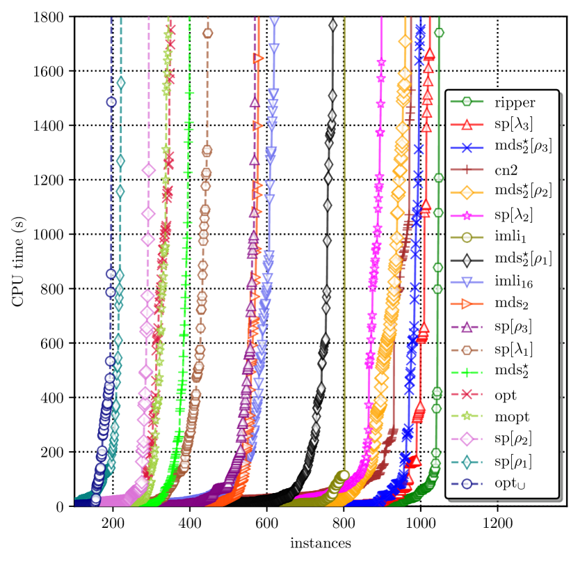
1(a) shows the performance of the considered competitors on the complete set of benchmark instances. As one can observe, ripper outperforms all the other tools and is able to train a classifier for 1048 of the considered datasets given the 1800s time limit. The proposed MaxSAT models for sparse decision sets sp$[\lambda_{3}]$ and mds${}_{2}^{\star}[\rho_{3}]$ (which are the configurations with the largest constant parameters) come second and third with 1024 and 1000 instances solved, respectively. The fourth place is taken by cn2, which can successfully deal with 975 datasets. The best configuration of imli, i.e. imli₁, finishes with 802 intances solved while the worst configuration imli₁₆ copes with only 620 datasets. Finally, the worst results are demonstrated by the approaches that target perfectly accurate decision sets opt, mopt, and opt_∪ but also by the sparse approaches with low regularized cost sp$[\rho_{1}]$ and sp$[\rho_{2}]$. For instance, opt_∪ solves only 196 instances. This should not come as surprise since the problem these tools target is computationally harder than what the other approaches solve.

Testing accuracy.

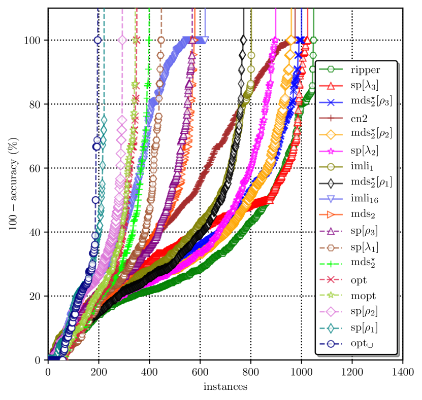
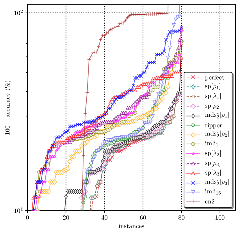
Having said that, perfectly accurate decision sets once computed have the highest possible accuracy. This is confirmed by 2(b), which depicts the accuracy obtained by all the tools for the datasets solved by all the tools. Indeed, as one can observe, the virtual perfect tool, which acts for all the approaches targeting perfectly accurate decision sets, i.e. opt, mopt, opt_∪, mds₂, and mds${}_{2}^{\star}$, beats the other tools in terms of test accuracy. Their average test accuracy on these datasets is $85.89\%$. In contrast, the worst accuracy is demonstrated by cn2 ($43.73\%$). Also, the average accuracy of ripper, sp$[\lambda_{3}]$, mds${}_{2}^{\star}[\rho_{3}]$, imli₁, imli₁₆ is $80.50\%$, $67.42\%$, $61.71\%$, $76.06\%$, $77.42\%$, respectively.

The picture changes drastically if we compare test accuracy on the complete set of benchmark datasets. This information is shown in 2(a). Here, if a tool does not solve an instance, its accuracy for the dataset is assumed to be $0\%$. Observe that the best accuracy is achieved by ripper ($68.13\%$ on average) followed by the sparse decision sets computed by sp$[\lambda_{3}]$ and mds${}_{2}^{\star}[\rho_{3}]$ ($60.91\%$ and $61.23\%$, respectively). The average accuracy achieved by imli₁ and imli₁₆ is $50.66\%$ and $28.26\%$ while the average accuracy of cn2 is $47.49\%$.

(a) Solution quality

(b) Accuracy

Figure 4: Comparison of sp$[\lambda_{3}]$ and imli₁.

Testing interpretability (size).

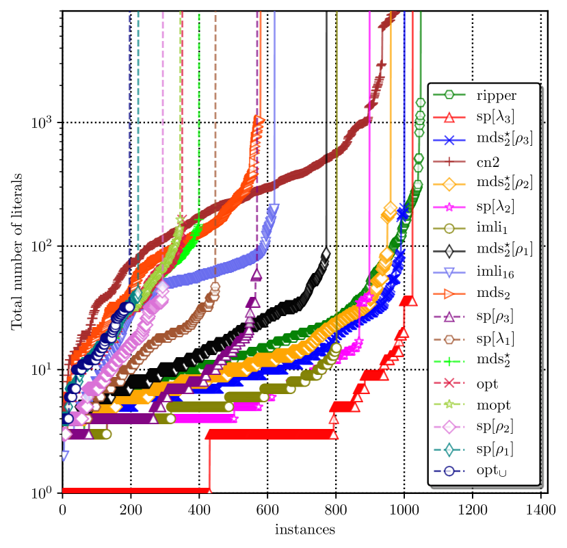
From the perspective of interpretability, the smaller a decision set is the easier it is for a human decision maker to comprehend. This holds for the number of rules in a decision set but also (and more importantly) for the total number of literals used. 1(b) depicts a cactus plots illustrating the size of solutions in terms of the number of literals obtained by each of the considered competitors. A clear winner here is sp$[\lambda_{3}]$. As can be observed, for more than 400 datasets, decision sets of sp$[\lambda_{3}]$ consist of only one literal. Another bunch of almost 400 datasets are represented by sp$[\lambda_{3}]$ with 3 literals. Getting these small decision sets is a striking achievement in light of the overall high accuracy reached by sp$[\lambda_{3}]$. The average size of solutions obtained by sp$[\lambda_{3}]$ is $4.18$. Note that imli₁ gets close to this with $5.57$ literals per dataset on average although it always compute only one rule. In clear contrast with this, the average solution size of ripper is $35.14$ while the average solution of imli₁₆ has $46.29$ literals. Finally, the result of cn2 is $598.05$ literals.

It is not surprising that perfectly accurate decision sets, i.e. those computed by opt, opt_∪, mopt, as well as mds₂ and mds${}_{2}^{\star}$, in general tend to be larger. It is also worth mentioning that mds${}_{2}^{\star}[\rho_{3}]$ obtains sparse decision sets of size $14.52$ on average while the original (non-sparse) version gets $40.70$ literals per solution.

A few more details.

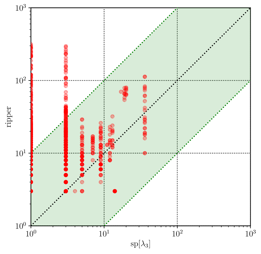
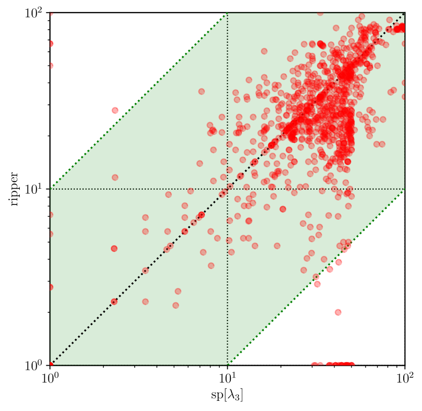
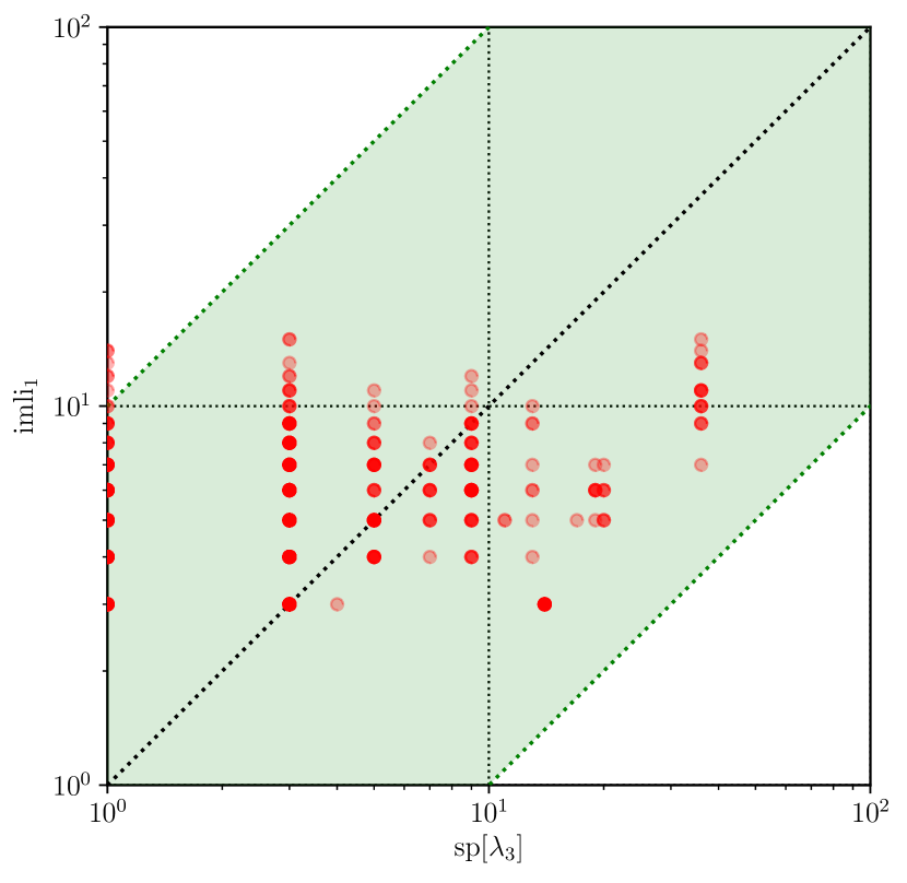
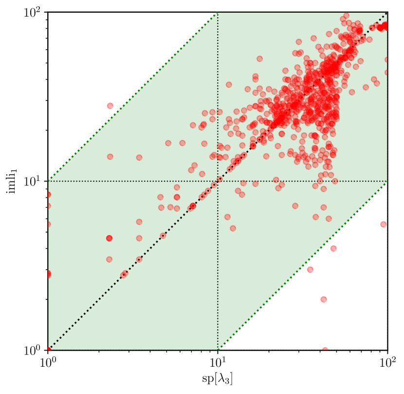
Figure 3 and Figure 4 detail a comparison of sp$[\lambda_{3}]$ with ripper and imli₁, respectively. All these plots are obtained for the datasets solvable by each pair of competitors. Concretely, as can be seen in 4(a) and 4(b), the size and accuracy of sp$[\lambda_{3}]$ and imli₁ are comparable. However, as imli₁ computes solutions representing only one class and it is significantly outperformed by sp$[\lambda_{3}]$, the latter approach is deemed a better alternative. Furthermore and although the best performance overall is demonstrated by ripper, its accuracy is comparable with the accuracy of sp$[\lambda_{3}]$ (see 3(b)) but the size of solutions produced by ripper can be several orders of magnitude larger than the size of solutions of its rival, as one can observe in 3(a).

Finally, a crucial observation to make is that since both RIPPER and IMLI compute a representation for one class only, they cannot provide a user with a succinct explanation for the instances of other (non-computed) classes. Indeed, an explanation in that case includes the negation of the complete decision set. This is in clear contrast with our work, which provides a user with a succinct representation of every class of the dataset.

6 Conclusion

We have introduced the first approach to build decision sets by directly minimizing the total number of literals required to describe them. The approach can build perfect decision sets that match the training data exactly, or sparse decision sets that trade off accuracy on training data for size. Experiments show that sparse decision sets can be preferred to perfectly accurate decision sets. This is caused by (1) their high accuracy overall and (2) the fact that they are much easier to compute. Second, it is not surprising that the regularization cost significantly affects the efficiency of sparse decision sets – the smaller the cost is, the harder it is compute the decision set and the more accurate the result decision set is. This fact represents a reasonable trade-off that can be considered in practice. Note that points 1 and 2 hold for the models proposed in this paper but also for the sparse variants of prior work targeting minimization of the number of rules [31]. Third, although heuristic methods like RIPPER may scale really well and produce accurate decision sets, their solutions tend to be much larger than sparse decision sets, which makes them harder to interpret. All in all, the proposed approach to sparse decision sets embodies a viable alternative to the state of the art represented by prior logic-based solutions [31, 39, 20] as well as by efficient heuristic methods [13, 12, 11].

There are number of interesting directions to extend this work. There is considerable symmetry in the models we propose, and while we tried adding symmetry breaking constraints to improve the models, what we tried did not make a significant difference. This deserves further exploration. Another interesting direction for future work is to consider other measures of interpretability, for example the (possibly weighted) average length of a decision rule, where we are not concerned about the total size of the decision set, but rather its succinctness in describing any particular instance.

Acknowledgments

This work is partially supported by the Australian Research Council through Discovery Grant DP170103174.

References

- [1] R. Asín, R. Nieuwenhuis, A. Oliveras, and E. Rodríguez-Carbonell. Cardinality networks and their applications. In SAT, pages 167–180, 2009.
- [2] G. Audemard, J. Lagniez, and L. Simon. Improving Glucose for incremental SAT solving with assumptions: Application to MUS extraction. In SAT, pages 309–317, 2013.
- [3] Australian Government. Artificial Intelligence Roadmap. https://data61.csiro.au/en/Our-Research/Our-Work/AI-Roadmap, November 2019.
- [4] D. Baehrens, T. Schroeter, S. Harmeling, M. Kawanabe, K. Hansen, and K. Müller. How to explain individual classification decisions. Journal of Machine Learning Research, 11:1803–1831, 2010.
- [5] O. Bailleux and Y. Boufkhad. Efficient CNF encoding of Boolean cardinality constraints. In CP, pages 108–122, 2003.
- [6] C. Barnhart, E. L. Johnson, G. L. Nemhauser, M. W. P. Savelsbergh, and P. H. Vance. Branch-and-price: Column generation for solving huge integer programs. Oper. Res., 46(3):316–329, 1998.
- [7] K. E. Batcher. Sorting networks and their applications. In AFIPS, volume 32, pages 307–314, 1968.
- [8] C. Bessiere, E. Hebrard, and B. O’Sullivan. Minimising decision tree size as combinatorial optimisation. In CP, pages 173–187, 2009.
- [9] A. Biere, M. Heule, H. van Maaren, and T. Walsh, editors. Handbook of Satisfiability. IOS Press, 2009.
- [10] L. Breiman, J. H. Friedman, R. A. Olshen, and C. J. Stone. Classification and Regression Trees. Wadsworth, 1984.
- [11] P. Clark and R. Boswell. Rule induction with CN2: some recent improvements. In EWSL, pages 151–163, 1991.
- [12] P. Clark and T. Niblett. The CN2 induction algorithm. Machine Learning, 3:261–283, 1989.
- [13] W. W. Cohen. Fast effective rule induction. In ICML, pages 115–123, 1995.
- [14] A. Darwiche. Three modern roles for logic in AI. In PODS, pages 229–243. ACM, 2020.
- [15] S. Dash, O. Günlük, and D. Wei. Boolean decision rules via column generation. In NeurIPS, page 4660–4670, 2018.
- [16] F. Doshi-Velez and B. Kim. A roadmap for a rigorous science of interpretability. CoRR, abs/1702.08608, 2017.
- [17] EU Data Protection Regulation. Regulation (EU) 2016/679 of the European Parliament and of the Council. http://eur-lex.europa.eu/legal-content/EN/TXT/PDF/?uri=CELEX:32016R0679&from=en, 2016.
- [18] R. Evans and E. Grefenstette. Learning explanatory rules from noisy data. J. Artif. Intell. Res., 61:1–64, 2018.
- [19] J. Fürnkranz, D. Gamberger, and N. Lavrac. Foundations of Rule Learning. Springer, 2012.
- [20] B. Ghosh and K. S. Meel. IMLI: an incremental framework for maxsat-based learning of interpretable classification rules. In AIES, pages 203–210. ACM, 2019.
- [21] B. Goodman and S. R. Flaxman. European Union regulations on algorithmic decision-making and a ”right to explanation”. AI Magazine, 38(3):50–57, 2017.
- [22] R. Guidotti, A. Monreale, F. Giannotti, D. Pedreschi, S. Ruggieri, and F. Turini. Factual and counterfactual explanations for black box decision making. IEEE Intelligent Systems, 34(6):14–23, 2019.
- [23] R. Guidotti, A. Monreale, S. Ruggieri, F. Turini, F. Giannotti, and D. Pedreschi. A survey of methods for explaining black box models. ACM Comput. Surv., 51(5):93:1–93:42, 2019.
- [24] D. Gunning and D. Aha. DARPA’s explainable artificial intelligence (XAI) program. AI Magazine, 40(2):44–58, 2019.
- [25] J. Han, M. Kamber, and J. Pei. Data Mining: Concepts and Techniques, 3rd edition. Morgan Kaufmann, 2012.
- [26] A. Ignatiev. Towards trustable explainable AI. In IJCAI, pages 5154–5158, 2020.
- [27] A. Ignatiev, A. Morgado, and J. Marques-Silva. PySAT: A Python toolkit for prototyping with SAT oracles. In SAT, pages 428–437, 2018.
- [28] A. Ignatiev, A. Morgado, and J. Marques-Silva. RC2: an efficient maxsat solver. J. Satisf. Boolean Model. Comput., 11(1):53–64, 2019.
- [29] A. Ignatiev, N. Narodytska, and J. Marques-Silva. Abduction-based explanations for machine learning models. In AAAI, pages 1511–1519, 2019.
- [30] A. Ignatiev, N. Narodytska, and J. Marques-Silva. On relating explanations and adversarial examples. In NeurIPS, pages 15857–15867, 2019.
- [31] A. Ignatiev, F. Pereira, N. Narodytska, and J. Marques-Silva. A SAT-based approach to learn explainable decision sets. In IJCAR, pages 627–645, 2018.
- [32] M. I. Jordan and T. M. Mitchell. Machine learning: Trends, perspectives, and prospects. Science, 349(6245):255–260, 2015.
- [33] A. P. Kamath, N. Karmarkar, K. G. Ramakrishnan, and M. G. C. Resende. A continuous approach to inductive inference. Math. Program., 57:215–238, 1992.
- [34] H. Lakkaraju, S. H. Bach, and J. Leskovec. Interpretable decision sets: A joint framework for description and prediction. In KDD, pages 1675–1684, 2016.
- [35] Y. LeCun, Y. Bengio, and G. Hinton. Deep learning. nature, 521(7553):436, 2015.
- [36] O. Li, H. Liu, C. Chen, and C. Rudin. Deep learning for case-based reasoning through prototypes: A neural network that explains its predictions. In AAAI, February 2018.
- [37] Z. C. Lipton. The mythos of model interpretability. Commun. ACM, 61(10):36–43, 2018.
- [38] S. M. Lundberg and S. Lee. A unified approach to interpreting model predictions. In NIPS, pages 4765–4774, 2017.
- [39] D. Malioutov and K. S. Meel. MLIC: A maxsat-based framework for learning interpretable classification rules. In CP, pages 312–327, 2018.
- [40] T. M. Mitchell. Machine learning. McGraw-Hill, 1997.
- [41] V. Mnih, K. Kavukcuoglu, D. Silver, A. A. Rusu, J. Veness, M. G. Bellemare, A. Graves, M. Riedmiller, A. K. Fidjeland, G. Ostrovski, et al. Human-level control through deep reinforcement learning. Nature, 518(7540):529, 2015.
- [42] D. Monroe. AI, explain yourself. Commun. ACM, 61(11):11–13, 2018.
- [43] G. Montavon, W. Samek, and K. Müller. Methods for interpreting and understanding deep neural networks. Digital Signal Processing, 73:1–15, 2018.
- [44] N. Narodytska, A. Ignatiev, F. Pereira, and J. Marques-Silva. Learning optimal decision trees with SAT. In IJCAI, pages 1362–1368, 2018.
- [45] Orange, a component-based data mining framework. https://orange.biolab.si/.
- [46] F. Pedregosa and et al. Scikit-learn: Machine learning in Python. Journal of Machine Learning Research, 12:2825–2830, 2011.
- [47] J. R. Quinlan. C4.5: Programs for machine learning. Morgan Kauffmann, 1993.
- [48] M. T. Ribeiro, S. Singh, and C. Guestrin. ”Why should I trust you?”: Explaining the predictions of any classifier. In KDD, pages 1135–1144, 2016.
- [49] M. T. Ribeiro, S. Singh, and C. Guestrin. Anchors: High-precision model-agnostic explanations. In AAAI, 2018.
- [50] R. L. Rivest. Learning decision lists. Machine Learning, 2(3):229–246, 1987.
- [51] SAT-based miner of smallest size decision sets. https://github.com/alexeyignatiev/minds.
- [52] A. Shih, A. Choi, and A. Darwiche. A symbolic approach to explaining bayesian network classifiers. In IJCAI, pages 5103–5111, 2018.
- [53] C. Sinz. Towards an optimal CNF encoding of Boolean cardinality constraints. In CP, pages 827–831, 2005.
- [54] G. S. Tseitin. On the complexity of derivation in propositional calculus. Studies in Constructive Mathematics and Mathematical Logic, Part II, pages 115–125, 1968.
- [55] UCI Machine Learning Repository. https://archive.ics.uci.edu/ml.
- [56] Ruleset covering algorithms for transparent machine learning. https://github.com/imoscovitz/wittgenstein.