Tutte polynomial, complete invariant, and theta series

Abstract.

In this study, we present two results that relate Tutte polynomials. First, we provide new and complete polynomial invariants for graphs. We note that the number of variables of our polynomials is one. Second, let $L_{1}$ and $L_{2}$ be two non-isomorphic lattices. We state that $L_{1}$ and $L_{2}$ are theta series equivalent if those theta series are the same. The problem of identifying theta series equivalent lattices is discussed in Prof. Conway’s book The Sensual (Quadratic) Form with the title “Can You Hear the Shape of a Lattice?” In this study, we present a method to find theta series equivalent lattices using matroids and their Tutte polynomials.

1. Introduction

In this study, we provide two results that relate the Tutte polynomials.

The first result is as follows: In [9], de la Harpe and Jones introduced graph-invariant polynomials. We refer to these polynomials as $n$-state polynomials.

The main focus of this paper is on non-directed graphs. Let $G$ be a graph and $X$ be a finite set with $n$ elements. $W_{n}=(x_{ij})$ is an $|X|\times|X|$ symmetric matrix indexed by the elements of $X$. We assume that $X=\{1,2,\ldots,n\}$ and $x_{ij}$ are variables. Moreover, let $\sigma:V(G)\rightarrow X$ be a state function. Subsequently, the $n$-state polynomials with $n(n+1)/2$ variables are defined as follows:

Definition 1.1 ([9]).

$$Z_{W_{n}}(G)=\sum_{\sigma:{\rm state}}\prod_{uv\in E(G)}W_{n}(\sigma(u),\sigma(v)),$$

where $\sigma$ runs over all state functions.

The special values of these polynomials are approximately the same as certain known polynomial invariants for graphs. For example, let

$$W_{{\rm Negami}}=\begin{pmatrix}x_{1}+y&y&\cdots&y\\ y&x_{1}+y&\cdots&y\\ \vdots&\vdots&\ddots&\vdots\\ y&y&\cdots&x_{1}+y\end{pmatrix}.$$

Then, $Z_{W_{\rm Negami}}(G)$ are known as Negami polynomials [13]. In [15], Oxley demonstrated that $Z_{W_{\rm Negami}}(G)$ is essentially equivalent to the Tutte polynomials [17, 18, 19]. Therefore, $n$-state polynomials are a generalization of the Tutte polynomials.

Moreover, let $W_{{\rm extNegami}}=(x_{ij})$,

$$x_{ij}=\left\{\begin{array}[]{l}x_{i}+y\ (i=j<n),\\ x_{n}+y\ (i=j\geq n),\\ y.\end{array}\right.$$

Then, $Z_{W_{\rm extNegami}}(G)$ are known as extended Negami polynomials [14].

In this study, we demonstrate that $n$-state polynomials are complete invariants for graphs.

Theorem 1.1.

The $n$-state polynomials $\{Z_{W_{n}}(G)\}_{n=1}^{\infty}$ are complete invariants for graphs.

According to the proof of Theorem 1.1, for $n\geq 2$, a graph $G$ with $n$ vertices is determined by the $n$-state polynomials, which have $n(n+1)/2$ variables. In this study, we consider the following problems:

Problem 1.1.

Let $\mathcal{G}$ be a set of certain graphs. Is there a polynomial invariant (hopefully equivalent to the one from the $n$-state polynomial) such that the polynomials determine any graph $G\in\mathcal{G}$ with $n$ vertices and a number of variables less than $n(n+1)/2$?

The first purpose of this study is to introduce polynomial invariants for graphs and to provide an answer to Problem 1.1. The number of variables of our polynomials is one. Furthermore, for any given graph $G$, if the degree of our polynomial is sufficiently large, then the set of terms of our polynomial is one-to-one corresponding to the set of terms of the $n$-state polynomial with the same degree. We refer to such polynomials as pseudo $n$-state polynomials, denoted by $Z_{\widetilde{W}_{n}}(G)$, which are explained in the following.

For $\ell\in\mathbb{N}$, we denote the $\ell$-th prime number as $P(\ell)$. We set the functions $a(i)$ on $\mathbb{N}$ and $b(i,j)$ on $\mathbb{N}^{2}$ such that

$$a(i,j):=\left(\frac{i(i+1)}{2}+(j-i)\right).$$

Let $\widetilde{W}_{n}=(\widetilde{W}_{n}(i,j))$ be the $n\times n$ symmetric matrix such that, for $i\geq j$,

$$\widetilde{W}_{n}(i,j):=\left\{\begin{array}[]{l}P(n^{na(i,i)})x^{P(n^{na(i,i)})}\ (\mbox{if }i=j),\\ P(n^{na(i,j)})x^{P(n^{na(i,j)})}\ (\mbox{if }i>j).\end{array}\right.$$

Next, we present the definition of the pseudo $n$-state polynomials:

Definition 1.2.

Let $\sigma:V(G)\rightarrow X$ be a state function. Then, the pseudo $n$-state polynomials are defined as follows:

$$Z_{\widetilde{W}_{n}}(G)=\sum_{\sigma:{\rm state}}\prod_{uv\in E(G)}\widetilde{W}_{n}(\sigma(u),\sigma(v)),$$

where $\sigma$ runs over all state functions.

We note that the number of variables of our polynomials is one. For example, for $n=2$,

$$\widetilde{W}_{2}=\begin{pmatrix}7x^{7}&53x^{53}\\ 53x^{53}&311x^{311}\end{pmatrix}$$

and for $n=3$,

$$\widetilde{W}_{3}=\begin{pmatrix}103x^{103}&5519x^{5519}&7867547x^{7867547}\\ 5519x^{5519}&220861x^{220861}&262960091x^{262960091}\\ 7867547x^{7867547}&262960091x^{262960091}&8448283757x^{8448283757}\end{pmatrix}.$$

Then, the pseudo $2$-state polynomial for the complete graph $K_{2}$ is

$$Z_{\widetilde{W}_{2}}(K_{2})=311x^{311}+106x^{53}+7x^{7}$$

and the pseudo $3$-state polynomial for the complete graph $K_{3}$ is

$$Z_{\widetilde{W}_{3}}(K_{3}) =1752546015417169494746495151x^{8974203939}$$

$$+1568803100908626481902639x^{8464018851}$$

$$+602983567540694711837927399093x^{25344851271}$$

$$+45816295551192560609823x^{526141043}$$

$$+68507927876961253578x^{270833157}$$

$$+19126573401337581x^{15735197}$$

$$+10773507110137381x^{662583}+20181854789463x^{231899}$$

$$+9411942549x^{11141}+1092727x^{309}.$$

The first main result in this paper is as follows:

Theorem 1.2.

The pseudo $n$-state polynomial $\{Z_{\widetilde{W}_{n}}\}_{n=1}^{\infty}$ is a complete invariant for graphs.

In the following, we present the second result of the study. Let $L_{1}$ and $L_{2}$ be two non-isomorphic lattices. We state that $L_{1}$ and $L_{2}$ are theta series equivalent if those theta series are the same:

$$\theta_{L_{1}}(q)=\theta_{L_{2}}(q).$$

The problem of determining theta series equivalent lattices is discussed in Prof. Conway’s book [4] under the title “Can You Hear the Shape of a Lattice?”

Problem 1.2 ([4, Can You Hear the Shape of a Lattice?]).

Finding theta series equivalent lattices.

For example, it is well known, as per the example of Milnor, that $E_{8}^{2}$ and $D_{16}^{+}$ are theta series equivalent [4, 5], and several examples are provided in [4].

In this study, we present a method to find theta series equivalent lattices using matroids and their Tutte polynomials. The second main result is as follows:

Theorem 1.3.

Let $d\in\{24,27,30,33,35,36,38,39,41,42\}\cup\{i\in\mathbb{Z}\mid i\geq 44\}$. Then, there exist non-isomorphic lattices of rank $4d$ with the same theta series.

Remark 1.1.

Prior to concluding this section, we provide a remark. The relationships and analogies among codes, lattices, and vertex operator algebras are well known in the algebraic combinatorics community. However, the proof of Theorem 1.3 uses the relationships among matroids, codes, and lattices. We remark that there may be a rich theory behind the matroids and the three objects codes, lattices, and vertex operator algebras.

The remainder of this paper is organized as follows: In Section 2, we summarize basic facts of matroids, codes, and lattices. In Section 3, we provide the proofs of Theorems 1.1 and 1.2. In Section 4, we provide the proof of Theorem 1.3. Finally, in Section 5, we present several remarks.

All computer calculations in this study were performed with the aid of Magma [1] and Mathematica [21].

2. Preliminaries

In this section, we summarize basic facts of matroids, codes, and lattices.

2.1. Matroids

Let $E$ be a set. A matroid $M$ on $E=E(M)$ is a pair $(E,\mathcal{I})$, where $\mathcal{I}$ is a non-empty family of subsets of $E$ with the following properties:

$$\begin{cases}\mbox{(i)}&\mbox{ if }I\in\mathcal{I}\mbox{ and }J\subset I,\mbox{ then }J\in\mathcal{I};\\ \mbox{(ii)}&\mbox{ if }I_{1},I_{2}\in\mathcal{I}\mbox{ and }|I_{1}|<|I_{2}|,\\ &\mbox{ then there exists }e\in I_{2}\setminus I_{1}\\ &\mbox{ such that }I_{1}\cup\{e\}\in\mathcal{I}.\end{cases}$$

Each element of the set $\mathcal{I}$ is known as an independent set. A matroid $(E,\mathcal{I})$ is isomorphic to another matroid $(E^{\prime},\mathcal{I}^{\prime})$ if there exists a bijection $\varphi$ from $E$ to $E^{\prime}$ such that $\varphi(I)\in\mathcal{I}^{\prime}$ holds for each member $I\in\mathcal{I}$, and $\varphi^{-1}(I^{\prime})\in\mathcal{I}$ holds for each member $I^{\prime}\in\mathcal{I}^{\prime}$.

It follows from the second axiom that all maximal independent sets in a matroid $M$ take the same cardinality, known as the rank of $M$. These maximal independent sets $\mathcal{B}(M)$ are referred to as the bases of $M$. The rank $\rho(A)$ of an arbitrary subset $A$ of $E$ is the cardinality of the largest independent set contained in $A$.

We provide examples below.

Example 2.1.

Let $A$ be a $k\times n$ matrix over a finite field $\mathbb{F}_{q}$. This results in a matroid $M$ on the set

$$E={\{z\in\mathbb{Z}\mid 1\leq z\leq n\}},$$

in which the set $\mathcal{I}$ is independent if and only if the family of columns of $A$ with indices belonging to $\mathcal{I}$ is linearly independent. Such a matroid is called a vector matroid.

Example 2.2.

Let $G=(V,E)$ be a non-directed finite graph, where $V$ is the vertex set of $G$ and $E$ is the edge set of $G$. Let $\mathcal{I}$ be the set of all subsets $A$ of $E$, such that the graph $(V,A)$ is acyclic. Then, $(E,\mathcal{I})$ is a matroid. Such a matroid is known as graphic and is denoted by $M(G)$.

The following fact is used in the proof of Theorem 1.3:

Fact 2.1.

The incidence matrix of $M(G)$ provides the vector matroid over $\mathbb{F}_{2}$, which is isomorphic to $M(G)$ as matroids.

The classification of matroids is one of the most important problems in the theory of matroids. The Tutte polynomials are a tool for classifying the matroids. Let $M$ be a matroid on the set $E$ with a rank function $\rho$. The Tutte polynomial of $M$ is defined as follows [17, 18, 19]:

$$T(M) :=T(M;x,y)$$

$$:=\sum_{A\subset E}(x-1)^{\rho(E)-\rho(A)}(y-1)^{|A|-\rho(A)}.$$

It can easily be demonstrated that $T(M;x,y)$ is a matroid invariant. Two matroids are $T$-equivalent if their Tutte polynomials are equivalent. It is well known that there exist two inequivalent matroids, which are $T$-equivalent (for example, see [20, p. 269] or Section 4), and these examples are key facts for the proof of Theorem 1.3.

2.2. Codes

Let $\mathbb{F}_{2}$ be the finite field of two elements. A linear code $C$ with length $n$ is a linear subspace of $\mathbb{F}_{2}^{n}$. An inner product $({x},{y})$ on $\mathbb{F}_{2}^{n}$ is given by

$$(x,y)=\sum_{i=1}^{n}x_{i}y_{i},$$

where $x,y\in\mathbb{F}_{q}^{n}$ with $x=(x_{1},x_{2},\ldots,x_{n})$ and $y=(y_{1},y_{2},\ldots,y_{n})$. The dual of the linear code $C$ is defined as follows:

$$C^{\perp}=\{{y}\in\mathbb{F}_{2}^{n}\mid({x},{y})=0\text{ for all }{x}\in C\}.$$

A linear code $C$ is known as self-dual if $C=C^{\perp}$. For $x\in\mathbb{F}_{2}^{n}$, the weight $\operatorname{wt}(x)$ is the number of its nonzero components. A self-dual code $C$ is doubly even if all codewords of $C$ have a weight that is divisible by four.

Let $C$ be a linear code of length $n$. The weight enumerator associated with $C$ is

$$w_{C}(x,y)=\sum_{c\in C}x^{n-\operatorname{wt}(c)}y^{\operatorname{wt}(c)}.$$

For example, let $C$ be a doubly even self-dual code. Then,

$$w_{C}(x,y)\in\mathbb{C}[P_{8},P_{24}],$$

where $P_{8}=x^{8}+14x^{4}y^{4}+y^{8},P_{24}=x^{4}y^{4}(x^{4}-y^{4})^{4}$ [5, 6].

2.3. Lattices

A lattice in $\mathbb{R}^{n}$ is a subgroup $L\subset\mathbb{R}^{n}$ with the property that there exists a basis $\{e_{1},\ldots,e_{n}\}$ of $\mathbb{R}^{n}$ such that $L=\mathbb{Z}e_{1}\oplus\cdots\oplus\mathbb{Z}e_{n}$. $n$ is known as the rank of $L$. The dual lattice of $L$ is the lattice

$$L^{\sharp}:=\{y\in\mathbb{R}^{n}\mid(y,x)\in\mathbb{Z},\ \forall x\in L\},$$

where $(x,y)$ is the standard inner product. A lattice $L$ is integral if $(x,y)\in\mathbb{Z}$ for all $x$, $y\in L$. An integral lattice $L$ is referred to as even if $(x,x)\in 2\mathbb{Z}$ for all $x\in L$. An integral lattice $L$ is referred to as unimodular if $L^{\sharp}=L$.

The norm of a vector $x$ is defined as $(x,x)$. A unimodular lattice with even norms is said to be even. An $n$-dimensional even unimodular lattice exists if and only if $n\equiv 0\pmod{8}$. For example, the unique even unimodular lattice of rank $8$, namely $E_{8}$, exists, and only two even unimodular lattices of rank $16$ exist, namely $E_{8}^{2}$ and $D_{16}^{+}$, which we mentioned as Milnor’s example of Problem 1.2. Moreover, the unique even unimodular lattice without roots of rank $24$ is the Leech lattice $\Lambda_{24}$.

Let $\mathbb{H}:=\{z\in\mathbb{C}\mid{\rm Im}(z)>0\}$ be the upper half-plane.

Definition 2.1.

For an integral lattice in $\mathbb{R}^{n}$, the function on $\mathbb{H}$ defined by

$$\theta_{L}(q):=\sum_{x\in L}e^{\pi iz(x,x)}=\sum_{x\in L}q^{(x,x)}$$

is known as the theta series of $L$, where $q=e^{\pi iz}$.

For example, we consider an even unimodular lattice $L$. Then, the theta series $\theta_{L}(q)$ of $L$ is a modular form with respect to $SL_{2}(\mathbb{Z})$. More precisely, we have

$$\theta_{L}\in\mathbb{C}[E_{4},\Delta]$$

where

$$E_{4}(q) :=1+240\sum_{n=1}^{\infty}\sigma_{3}(n)q^{2n},$$

$$E_{6}(q) :=1-504\sum_{n=1}^{\infty}\sigma_{5}(n)q^{2n},$$

$$\Delta(q) :=\frac{E_{4}(q)^{3}-E_{6}(q)^{2}}{1728}.$$

where $\sigma_{k-1}(n):=\sum_{d\mid n}d^{k-1}$ [5, 6].

3. Proofs of Theorems 1.1 and 1.2

3.1. Proof of Theorem 1.1

In this section, we prove Theorem 1.1.

Proof of Theorem 1.1.

We recover the graph structure of $G=(V,E)$ from the polynomials $\{Z_{W_{n}}(G)\}_{n=1}^{\infty}$.

First, we compute the number of the vertices $|V|$. According to [13, Corollary 2.2], it is possible to compute the number of vertices:

$$|V|=\log_{2}(Z_{W_{2}}(G;x_{11}\rightarrow 1,x_{12}\rightarrow 1,x_{22}\rightarrow 1)).$$

We denote the number of vertices as $n$.

Second, we demonstrate that $Z_{W_{n}}$ determines the graph structure. The reason is as follows: We seek a term

$$(\mbox{constant})\times x_{i_{11}i_{12}}^{e_{1}}x_{i_{21}i_{22}}^{e_{2}}\cdots x_{i_{m1}i_{m2}}^{e_{m}}$$

in $Z_{W_{n}}(G)$ such that

$$\sharp\{i_{11},i_{12},i_{21},i_{22},\ldots,i_{m1},i_{m2}\}$$

is the maximum among all of the terms. It can easily be observed that this term is expressed by a bijective state function $\sigma$. If

$$\{1,2,\ldots,n\}=\{i_{11},i_{12},i_{21},i_{22},\ldots,i_{m1},i_{m2}\},$$

$G$ is a graph with $n$ vertices

$$\{1,2,\ldots,n\},$$

and $i_{j1}$ and $i_{j2}$ are adjacent with $e_{j}$ edges.

If

$$\sharp\{1,2,\ldots,n\}>\sharp\{i_{11},i_{12},i_{21},i_{22},\ldots,i_{m1},i_{m2}\}$$

and assuming that

$$\{j_{1},\ldots,j_{\ell}\}:=\{1,2,\ldots,n\}\setminus\{i_{11},i_{12},i_{21},i_{22},\ldots,i_{m1},i_{m2}\},$$

$G$ is a graph with $n$ vertices

$$\{1,2,\ldots,n\}$$

and $\ell$ isolated vertices

$$\{j_{1},\ldots,j_{\ell}\},$$

such that $i_{j1}$ and $i_{j2}$ are adjacent with $e_{j}$ edges. This completes the proof of Theorem 1.1. ∎

3.2. Proof of Theorem 1.2

In this section, we prove Theorem 1.2.

Proof of Theorem 1.2.

We recover the graph structure from the polynomials $\{Z_{\widetilde{W}_{n}}(G)\}_{n=1}^{\infty}$.

First, we compute the number of edges $|E|$. It is possible to compute the number of edges as follows:

$$|E|=\log_{2}(Z_{\widetilde{W}_{1}}(G;x\rightarrow 1)).$$

We denote the number of edges of $G$ as $m$.

We demonstrate that $Z_{\widetilde{W}_{3m}}$ determines the graph structure. The reason is as follows: Let

$$Z_{\widetilde{W}_{3m}}(G)=\sum_{i=1}^{\ell_{G}}c(i)x^{i}.$$

For all $i\in\{1,\ldots,\ell_{G}\}$, we compute the prime factorization of $c(i)$ and seek the corresponding indices of $\widetilde{W}_{3m}$ (say, $I(c(i))$). For example, we recall that

$$\widetilde{W}_{3}=\begin{pmatrix}103x^{103}&5519x^{5519}&7867547x^{7867547}\\ 5519x^{5519}&220861x^{220861}&262960091x^{262960091}\\ 7867547x^{7867547}&262960091x^{262960091}&8448283757x^{8448283757}\end{pmatrix}.$$

Then, the pseudo $3$-state polynomial for the complete graph $K_{2}$ is

$$Z_{\widetilde{W}_{3}}(K_{2}) =8448283757x^{8448283757}+525920182x^{262960091}$$

$$+15735094x^{7867547}+220861x^{220861}+11038x^{5519}+103x^{103}.$$

Because of $103=1\times 103$, the term $103x^{103}$ yields

$$I(103)=\{\{1,1\}\},$$

and because of $11038=2\times 5519$, the term $11038x^{5519}$ yields

$$I(11038)=\{\{1,2\}\}.$$

Let

$$\widetilde{I}(c(i))=\{i\in\mathbb{N}\mid i\in I,I\in I(c(i))\setminus\{\{i,i\}\in\mathbb{N}^{2}\}\}$$

and $j$ be the index such that $\sharp\widetilde{I}(c(j))$ is the maximum for all

$$\{\widetilde{I}(c(i))\mid i\in\{1,\ldots,\ell_{G}\}\}.$$

We set $n^{\prime}:=\sharp\widetilde{I}(c(j))$. Thereafter, we recover the edges of $G$ as follows: We use $G^{\prime}$ to denote the subgraph of $G$ except for all isolated vertices.

Clearly we have that $|V(G^{\prime})|\leq 2|E(G^{\prime})|\leq 2m$. Let $p(i,j)x^{p(i,j)}$ denote the $(i,j)$-entry of $\widetilde{W}_{3m}$. Then we have

$$mp(i,i)<p(i+1,1)\textrm{~{}and~{}}mp(i,j-1)<p(i,j)$$

for every pair $(i,j)$ with $i\geq j$. Hence each term of $Z_{\widetilde{W}_{3m}}$ is one-to-one corresponding to a unique state upto automorphism of $G^{\prime}$.

$G^{\prime}$ is a graph with $n^{\prime}$ vertices

$$\{1,2,\ldots,n^{\prime}\}$$

and for

$$I(c(j))=\{\underbrace{\{i_{1},i_{2}\},\ldots,\{i_{1},i_{2}\}}_{e_{1,2}},\ldots\},$$

$i_{1}$ and $i_{2}$ are adjacent with $e_{1,2}$ edges.

Finally, we recover the number of isolated vertices. It can easily be observed that

$$c(j)=(3m)^{|V(G)|-|V(G^{\prime})|}\times|\operatorname{Aut}(G^{\prime})|.$$

Subsequently, we recover the number of isolated vertices: $|V(G)|-|V(G^{\prime})|$.

This completes the proof of Theorem 1.2. ∎

4. Proof of Theorem 1.3

In this section, we present the proof of Theorem 1.3. Prior to this, in Section 4.1, we provide a relationship between matroids and codes, and in Section 4.2, we present a relationship between codes and lattices.

4.1. Relationship between matroids and codes

In [7], a relationship between the weight enumerators of codes and the Tutte polynomials of matroids was presented.

Let $M$ be a vector matroid obtained from the $k\times n$ matrix $A$. Then, the row space of $A$ is a code over $\mathbb{F}_{2}$ of length $n$. We denote such a code as $C_{M}$. The Tutte polynomial of a vector matroid $M$ and the weight enumerator of $C_{M}$ exhibit the following relation:

Theorem 4.1 ([7]).

Let $M$ be a vector matroid on a set $E=\{1,\ldots,n\}$ over $\mathbb{F}_{2}$. Then,

$$w_{C_{M}}(x_{1},x_{2})=x_{2}^{n-\dim(C_{M})}(x_{1}-x_{2})^{\dim(C_{M})}T\left(M;\frac{x_{1}+x_{2}}{x_{1}-x_{2}},\frac{x_{1}}{x_{2}}\right).$$

4.2. Relationship between codes and lattices

We propose a method to construct lattices from codes over $\mathbb{F}_{2}$, which is referred to as Construction A [2, 8]. Let $\rho$ be a map from $\mathbb{Z}^{n}$ to $\mathbb{F}_{2}^{n}$ sending $(x_{i})$ to $(x_{i}\pmod{2})$. If $C$ is a $\mathbb{F}_{2}$ code of length $n$, we have an $n$-dimensional unimodular lattice

$$L_{C}=\frac{1}{\sqrt{2}}\{x\in\mathbb{Z}^{n}\mid\rho(x)\in C\}.$$

The following is an established fact [6]:

Theorem 4.2 ([6]).

Let $C$ be a code and $L_{C}$ be a lattice obtained from $C$ by Construction A. Then,

$$w_{C}(\theta_{3},\theta_{2})=\theta_{L_{C}}(q),$$

where

$$\theta_{3}=\sum_{n\in\mathbb{Z}}q^{n^{2}},\theta_{2}=\sum_{n\in\mathbb{Z}+1/2}q^{n^{2}}.$$

We explain Milnor’s example of Problem 1.2 [5]. There exist non-isomorphic doubly even self-dual codes of length $16$, $e_{8}^{2}$ and $d_{16}^{+}$ [5]. Then, according to section 2.2, their weight enumerators are the same:

$$w_{e_{8}^{2}}(x,y)=w_{d_{16}^{+}}(x,y)=P_{8}^{2}=(x^{8}+14x^{4}y^{4}+y^{8})^{2}.$$

Moreover, we obtain the non-isomorphic unimodular lattices of rank $16$, $E_{8}^{2}=L_{e_{8}^{2}}$ and $D_{16}^{+}=L_{d_{16}^{+}}$, with the same theta series:

$$\theta_{E_{8}}(q) =\theta_{D_{16}^{+}}(q)$$

$$=w_{e_{8}^{2}}(\theta_{3},\theta_{2})=w_{d_{16}^{+}}(\theta_{3},\theta_{2})=(\theta_{3}^{8}+14\theta_{3}^{4}\theta_{2}^{4}+\theta_{2}^{8})^{2}=E_{4}(q).$$

Therefore, this example arises from the following concept:

Codes $\longrightarrow$ Lattices.

The main idea of the proof of Theorem 1.3 is that we add “Matriods” to the above diagram:

Matroids $\longrightarrow$ Codes $\longrightarrow$ Lattices.

Thus, first, we have non-isomorphic graphic matroids with the same Tutte polynomials, following which we obtain non-isomorphic codes and lattices, which have the same theta series. We explain this in further detail in the following section.

4.3. Proof of Theorem 1.3

In this section, we demonstrate the proof of Theorem 1.3.

Proof of Theorem 1.3.

Let $G_{1}$ and $G_{2}$ be the graphs in Figure 1 [3].

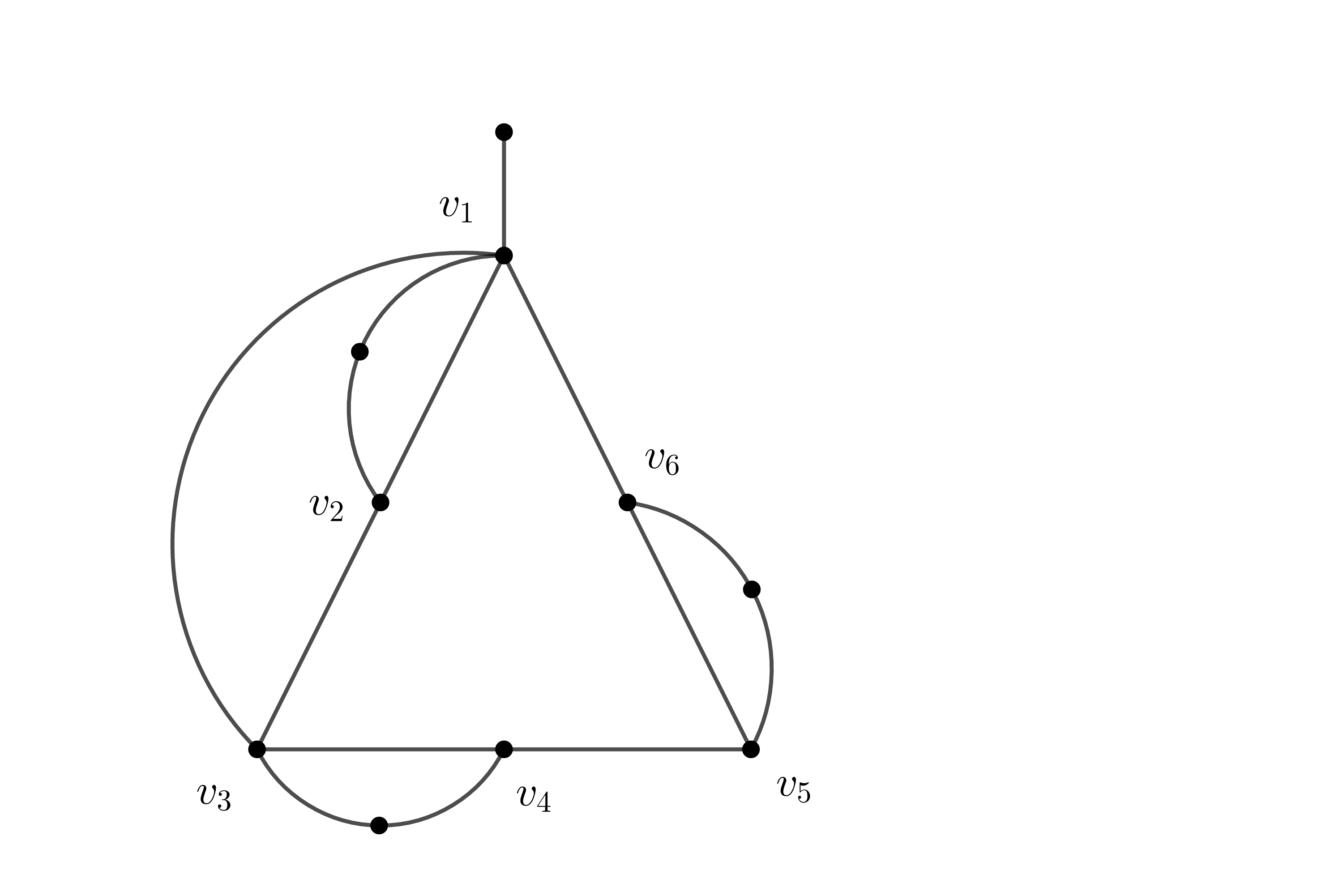
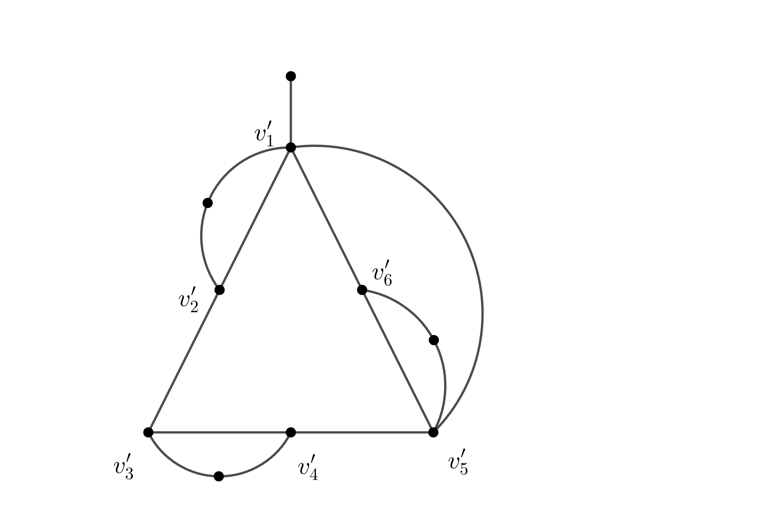
Figure 1. $G_{1}$ and $G_{2}$

Furthermore, for $i\in\{1,2\}$ and $n\in\mathbb{Z}_{\geq 0}$, let $G_{i}(n)=G_{i}\ast P_{n}$ be the joining of the graphs $G_{i}(n)$ and $P_{n}$, where $P_{n}$ indicates the path graph with $n$ edges. Note that the joining $G=G_{1}\ast G_{2}$ of graphs $G_{1}=(V_{1},E_{1})$ and $G_{2}=(V_{2},E_{2})$ is the graph union of the $G_{1}$ and $G_{2}$ together with all edges joining $V_{1}$ and $V_{2}$.

For $i\in\{1,2\}$ and $m\in\mathbb{Z}_{\geq 0}$, let $G_{i}(m,n)$ be the graphs with $m$ times edge subdivisions with respect to the edges:

$$v_{1}v_{2},v_{3}v_{4},v_{5}v_{6},v^{\prime}_{1}v^{\prime}_{2},v^{\prime}_{3}v^{\prime}_{4},v^{\prime}_{5}v^{\prime}_{6}.$$

We note that, for $i\in\{1,2\}$, the number of edges of $G_{i}(m,n)$ is $3m+11n+24$.

It was demonstrated in [3] that $G_{1}(m,n)$ and $G_{2}(m,n)$ are non-isomorphic graphic matroids with the same Tutte polynomials. For $i\in\{1,2\}$, let $M_{i}$ be the vector matroid with respect to the incident matrix of $G_{i}(m,n)$. Then, according to Fact 2.1 and Theorem 4.1, we can obtain the non-isomorphic codes $C_{M_{1}}$ and $C_{M_{2}}$ with length $3m+11n+24$ that have the same weight enumerator.

Let $\varphi:\mathbb{F}_{2}\rightarrow\mathbb{F}_{2}^{4}$ be a map such that

$$0\mapsto 0000,1\mapsto 1111.$$

For $i\in\{1,2\}$, we define a new code with length $4(3m+11n+24)$:

$$\widetilde{C}_{M_{i}}:=\{(\varphi(c_{i}))\mid(c_{i})\in{C}_{M_{i}}\}.$$

We note that $\widetilde{C}_{M_{i}}$ is doubly even. According to [10, 16] and Theorem 4.2, we can obtain the non-isomorphic lattices $L_{\widetilde{C}_{M_{1}}}$ and $L_{\widetilde{C}_{M_{2}}}$ with the same theta series.

The rank of $L_{\widetilde{C}_{M_{1}}}$ and $L_{\widetilde{C}_{M_{2}}}$ is $4(3m+11n+24)$. We remark that

$$3m+11n+24$$

represents the numbers

$$\{24,27,30,33,35,36,38,39,41,42\}\cup\{i\in\mathbb{Z}\mid i\geq 44\}.$$

This completes the proof of Theorem 1.3. ∎

5. Concluding remarks

We provide the following remarks:

1. According to the proof of Theorem 1.2, the pseudo $3m$-state polynomials recover the graph structure with a number of edges less than or equal to $m$. It is natural to ask whether there exists a function $f(n)$ on $n\in\mathbb{N}$ such that the polynomials with $f(n)$ variables recover the graph structure with a number of vertices less than or equal to $n$.

2. Problem: For $n\in\mathbb{N}$, determine the set of graphs $\mathcal{G}_{n}$ such that the pseudo $n$-state polynomials determine any graph $G\in\mathcal{G}_{n}$.

3. Problem: In [11, 12], we defined a complete invariant for matroids. For a graphic matroid, determine whether or not this invariant is a special value of $n$-state polynomials.

4. In the proof of Theorem 1.3, we demonstrated that $L_{\widetilde{C}_{M_{1}}}$ and $L_{\widetilde{C}_{M_{2}}}$ are non-isomorphic with rank $4d$, where

   $$d\in\{24,27,30,33,35,36,38,39,41,42\}\cup\{i\in\mathbb{Z}\mid i\geq 44\}.$$

   However, for

   $$d\in\{24,27,30,33,35\},$$

   we showed, with the aid of Magma, that $L_{{C}_{M_{1}}}$ and $L_{{C}_{M_{2}}}$ are non-isomorphic. Therefore, we have the following conjecture:

   Conjecture 5.1.

   $L_{{C}_{M_{1}}}$ and $L_{{C}_{M_{2}}}$, as defined in the proof of Theorem 1.3, are non-isomorphic.

   If Conjecture 5.1 is true,

   we obtain examples of Problem 1.2 for rank

   $$d\in\{24,27,30,33,35,36,38,39,41,42\}\cup\{i\in\mathbb{Z}\mid i\geq 44\}.$$

5. The Tutte polynomials of genus $g$ were defined in [11] and we discuss their properties in a forthcoming paper [12]. According to Theorem 4.1, there is a correspondence between the Tutte polynomials and weight enumerators.

   Thus, it is also natural to ask whether there is a correspondence between the Tutte polynomials and weight enumerators of genus $g$.

   It is well known that the weight enumerators of genus $g$ yield the Siegel theta series. Therefore, if such a correspondence exists, we may obtain examples whereby the non-isomorphic lattices have the same Siegel theta series.

6. Using the concept of this study and the following diagram:

   Matroids $\longrightarrow$ Codes $\longrightarrow$ Lattices $\longrightarrow$ Vertex operator (super) algebras,

   we may obtain the non-isomorphic vertex operator (super) algebras with the same trace function.

References

- [1] W. Bosma, J. Cannon and C. Playoust. The Magma algebra system. I. The user language, J. Symb. Comp. 24 (1997), 235–265.
- [2] E. Bannai, S.T. Dougherty, M. Harada and M. Oura, Type II codes, even unimodular lattices, and invariant rings, IEEE Trans. Inform. Theory 45 (1999), 1194–1205.
- [3] B. Bollobaś, L. Pebody, and O. Riordan, Contraction-deletion invariants for graphs, J. Combin. Theory Ser. B 80 (2000), no. 2, 320–345.
- [4] J.H. Conway, The sensual (quadratic) form. Carus Mathematical Monographs, 26. Mathematical Association of America, Washington, DC, 1997.
- [5] J.H. Conway and N.J.A. Sloane, Sphere Packing, Lattices and Groups (3rd ed.), Springer-Verlag, New York, 1999.
- [6] W. Ebeling, Lattices and codes, A course partially based on lectures by Friedrich Hirzebruch, Third edition, Advanced Lectures in Mathematics, Springer Spektrum, Wiesbaden, 2013.
- [7] C. Greene, Weight enumeration and the geometry of linear codes, Studia Appl. Math. 55 (1976), 119–128.
- [8] M. Harada, A. Munemasa, B. Venkov, Classification of ternary extremal self-dual codes of length , Math. Comp. 78 (2009), no. 267, 1787–1796.
- [9] P. de la Harpe, V.F.R. Jones, Graph invariants related to statistical mechanical models: examples and problems., J. Combin. Theory Ser. B 57 (1993), no. 2, 207–227.
- [10] M. Kitazume, T. Kondo, and I. Miyamoto, Even lattices and doubly even codes. J. Math. Soc. Japan 43 (1991), no. 1, 67–87.
- [11] T. Miezaki, M. Oura, T. Sakuma and H. Shinohara, A generalization of the Tutte polynomials. Proc. Japan Acad. Ser. A Math. Sci. 95 (2019), no. 10, 111–113.
- [12] T. Miezaki, M. Oura, T. Sakuma and H. Shinohara, The Tutte polynomials of genus , in preparation.
- [13] S. Negami, Polynomial invariants of graphs, Trans. Amer. Math. Soc. 299 (1987), no. 2, 601–622.
- [14] S. Negami, K. Kawagoe, Polynomial invariants of graphs with state models. Special Issue: Fifth Franco-Japanese Days (Kyoto, 1992)., Discrete Appl. Math. 56 (1995), no. 2–3, 323–331.
- [15] J.G. Oxley, A note on Negami’s polynomial invariants for graphs, Discrete Math. 76 (1989), no. 3, 279–281.
- [16] H. Shimakura, On isomorphism problems for vertex operator algebras associated with even lattices, Proc. Amer. Math. Soc. 140 (2012), 3333–3348.
- [17] W.T. Tutte, A ring in graph theory, Proc. Cambridge Philos. Soc., 43:26–40, 1947.
- [18] W.T. Tutte, A contribution to the theory of chromatic polynomials, Canadian J. Math., 6:80–91, 1954.
- [19] W.T. Tutte, On dichromatic polynomials, J. Combinatorial Theory, 2:301–320, 1967.
- [20] D.J.A. Welsh, Matroid Theory, Academic Press, London, 1976.
- [21] Wolfram Research, Inc., Mathematica, Version 11.2, Champaign, IL (2017).