justified

Invariant-based inverse engineering of time-dependent, coupled harmonic oscillators

Abstract

Two-dimensional systems with time-dependent controls admit a quadratic Hamiltonian modelling near potential minima. Independent, dynamical normal modes facilitate inverse Hamiltonian engineering to control the system dynamics, but some systems are not separable into independent modes by a point transformation. For these “coupled systems” 2D invariants may still guide the Hamiltonian design. The theory to perform the inversion and two application examples are provided: (i) We control the deflection of wave packets in transversally harmonic waveguides; and (ii) we design the state transfer from one coupled oscillator to another.

Introduction. Controlling the motional dynamics of quantum systems is of paramount importance for fundamental science and quantum-based technologies Kielpinski2002 . Often the external driving needs to be fast, but also gentle, to avoid excitations. Slow adiabatic driving is gentle in this sense, but it exposes the system for long times to control noise, heating, and perturbations. Shortcuts to adiabaticity (STA) are techniques to reach, via fast non-adiabatic routes, the results of slow adiabatic processes Torrontegui2013 ; Guery2019 . A distinction can be made between: STA methods that keep the structure of some Hamiltonian form and design the time dependence of the controls, e.g. using invariants Chen2010_063002 ; and those techniques that add new terms, e.g. counterdiabatic driving Demirplak2003 . Both may be useful depending on system-dependent practical considerations. A frequent problem with added terms is the difficulty to implement them, whereas a limitation of structure-preserving, invariant-based methods is that they need Hamiltonian-invariant pairs with specific forms, such as the Lewis-Leach family of Hamiltonian-invariant pairs Lewis1982 , to go beyond brute-force parameter optimization Torrontegui2013 ; Guery2019 .

The eigenvectors of Lewis-Riesenfeld “time-dependent invariants” Lewis1969 , with appropriate phase factors, are independent solutions of the Schrödinger equation and span a basis to expand any solution with constant expansion coefficients. These invariants are useful to inverse engineer the Hamiltonian and drive some desired dynamics Chen2010_063002 . The multiplicity of solutions for the trajectories of the control parameters, allows for adjustments or optimization with respect to different objectives or cost functions Ruschhaupt2012 . The multiplicity is also very helpful when several oscillators have to be controlled simultaneously Palmero2014 ; Palmero2015a .

This work extends the domain of systems that can be controlled by invariant-based inverse engineering. We shall deal with two-dimensional (2D) systems with quadratic Hamiltonians, found in particular in small-oscillation regimes of ultracold atom physics. In fact quadratic Hamiltonians are ubiquitous as they represent the systems near potential minima Urzua2019 . For time-independent Hamiltonians the dynamics is simple to describe and, possibly, manipulate by finding normal modes for effective uncoupled oscillators. This decomposition though, may not be possible if the Hamiltonian parameters depend on time. Lizuain et al. Lizuain2017 described the condition for which a point transformation of coordinates decouples the instantaneous modes leading to truly independent “dynamical normal modes” Palmero2014 for two time-dependent harmonic oscillators: the principal axes of the potential should not rotate in the 2D space.

When the two dynamical-mode motions separate, inverse engineering the dynamics to perform some fast operation free from final excitations is relatively easy: each of the time-dependent effective oscillators implies a one-dimensional Hamiltonian-invariant “Lewis-Leach” pair Lewis1982 for which inverse engineering can be performed. The two oscillators have to be driven simultaneously with common controls but, among the plethora of parameter trajectories, it is possible to find the ones that satisfy simultaneously the boundary conditions imposed on both oscillators. This strategy has been successfully applied to design the driving of different operations on two trapped ions such as transport or expansions Palmero2014 ; Palmero2015a , separation of two equal ions in double wells Palmero2015 , phase gates Palmero2017 , or dynamical exchange cooling Sagesser2020 .

If the effective potential rotates, the motions do not separate, so inverse engineering the external driving cannot in principle be done using two independent 1D Hamiltonian-invariant pairs. Solutions to the ensuing control problem exist that depend on the system and/or the operation, such as taking refuge in a perturbative regime Palmero2017 , adding terms to cancel the inertial effects Lizuain2017 , increasing the number of time-dependent controls to uncouple the modes Sagesser2020 , or using more complex, non-point transformations to find independent modes Lizuain2019a . Here we explore instead the use of 2D dynamical invariants associated with the coupled Hamiltonian.

Hamiltonian model. Consider the Hamiltonian

$$H(t)=\frac{{p}_{1}^{2}}{2}+\frac{{p}_{2}^{2}}{2}+\frac{1}{2}\omega_{1}^{2}(t){q}_{1}^{2}+\frac{1}{2}\omega_{2}^{2}(t){q}_{2}^{2}-{\gamma}(t){q}_{1}{q}_{2}.$$ (1)

We use throughout dimensionless variables such that no mass factors or $\hbar$ appear explicitly. Eq. (1) describes different physical systems, such as a single particle in a 2D potential, or two coupled harmonic oscillators on a line. Other systems different from (one or two) particles but driven by Hamiltonians of the form (1) are, e.g., coupled superconducting qubits Barends2013 ; Rol2019 ; Peropadre2013 ; Garcia-Ripoll2020 ; Chen2014 or optomechanical oscillators Kleckner_2011 ; Zhang2014 ; Aspelmeyer_2014 . All these systems are analogous to each other but, arguably, the single particle in a 2D potential is easiest to visualize so we shall use a terminology (such as longitudinal and transversal directions for principal axes, rotations…) borrowed from that system. Indeed, our first example, see below, deals with a single particle.

The Hamiltonian (1) may be instantaneously diagonalized by “rotated” variables Lizuain2017

$$\begin{pmatrix}q_{l}\\ q_{t}\end{pmatrix}=A(t)\begin{pmatrix}q_{1}\\ q_{2}\end{pmatrix},\hskip 17.07182pt\begin{pmatrix}p_{l}\\ p_{t}\end{pmatrix}=A(t)\begin{pmatrix}p_{1}\\ p_{2}\\ \end{pmatrix},$$ (2)

where ${A(t)=\begin{pmatrix}\cos\theta(t)&\sin\theta(t)\\ -\sin\theta(t)&\cos\theta(t)\\ \end{pmatrix}}$, and

$$\theta(t)=\frac{1}{2}\arctan\!{\left(\!\frac{2\gamma(t)}{\omega_{2}^{2}(t)-\omega_{1}^{2}(t)}\!\right)}.$$ (3)

Subscripts $l$ and $t$ stand for “longitudinal” and “transversal”. The original Hamiltonian, expressed in terms of the new variables, is

$$H = \frac{p_{l}^{2}}{2}+\frac{p_{t}^{2}}{2}+\frac{1}{2}\Omega_{l}^{2}q_{l}^{2}+\frac{1}{2}\Omega_{t}^{2}q_{t}^{2},$$ (4)

$$\Omega_{l}^{2} = {\left(\omega_{1}^{2}+\omega_{2}^{2}-\Lambda\right)}/{2},\,\,\,\,\,\,\Omega_{t}^{2}={\left(\omega_{1}^{2}+\omega_{2}^{2}+\Lambda\right)}/{2},$$ (5)

where $\Lambda(t)=\sqrt{4\gamma^{2}(t)+[\omega_{2}^{2}(t)-\omega_{1}^{2}(t)]^{2}}$.

The formal decoupling in Eq. (4) is a mirage. $H$ is not the Hamiltonian that describes the dynamics in the rotated variables $\{p_{l},p_{t},q_{l},q_{t}\}$ Goldstein2002 ; Lizuain2017 . In general the dependence of $A(t)$ on time couples dynamically the “instantaneous normal modes”, i.e., the normal modes that would separate the motion if the Hamiltonian kept for all times the values that the parameters have at a particular instant. In the moving frame the oscillators are coupled by a term proportional to $\dot{\theta}=d\theta/dt$ Lizuain2017 . Some peculiar, but physically significant relations between $\omega_{1}(t)$, $\omega_{2}(t)$, and $\gamma(t)$ can make $\theta(t)$ time independent. Here we consider instead the scenario where $\theta(t)$ changes with time. This is unavoidable if the process we want to implement implies boundary conditions for the parameters such that $\theta(0)\neq\theta(t_{f})$, as in the examples below.

2D Invariant. Urzúa et al. Urzua2019 , generalizing previous results in 1D Guasti2002 ; Guasti2003 and the work in Thylwe1998 for classical coupled oscillators, see also Castanos1994 , have recently found that the linear combination of operators (dots stand for time derivatives hereafter)

$$G(t)=u_{1}(t)p_{1}-\dot{u}_{1}(t)q_{1}+u_{2}(t)p_{2}-\dot{u}_{2}(t)q_{2},$$ (6)

satisfies the invariant equation $i\partial G/\partial t-[H,G]=0$, provided $u_{1}$ and $u_{2}$ satisfy

$$\ddot{u}_{1}+\omega_{1}^{2}(t)u_{1}=\gamma(t)u_{2},\;\;\;\;\;\ddot{u}_{2}+\omega_{2}^{2}(t)u_{2}=\gamma(t)u_{1},$$ (7)

which are classical equations of motion driven by a Hamiltonian (1). For any state driven by $H(t)$, $\langle G(t)\rangle$ is the sum of two Wronskians $W_{1}[u_{1}(t),\langle q_{1}\rangle(t)]+W_{2}[u_{2}(t),\langle q_{2}\rangle(t)]$, where all functions in their arguments evolve as Eq. (7). The geometrical meaning of $W_{i}(t)$ is an “oriented” phase-space area formed by phase-space points $U_{i}(t)=\{u_{i}(0),\dot{u}_{i}(t)\}$, $Q_{i}(t)=\{\langle q_{i}\rangle(t),\langle p_{i}\rangle(t)\}$ and the origin $\{0_{i},0_{i}\}$. We consider two phase spaces, $i=1,2$, one for each oscillator. $W_{i}(t)$ is plus or minus the triangle area $A_{i}(t)$ depending on whether going from $U_{i}$ to $Q_{i}$ needs an anticlockwise or clockwise displacement. For $\gamma=0$, the two areas (and Wronskians) remain constant in time. When $\gamma\neq 0$ the individual Wronskians are not conserved. The conserved quantities are now $W_{i}(t)-\int_{0}^{t}\dot{W}_{i}(t^{\prime})dt^{\prime}=W_{i}(0)$, i.e., the initial phase-space oriented areas. The added terms cancel each other, namely, $\dot{W}_{1}=-\dot{W}_{2}=(u_{1}\langle q_{2}\rangle-\langle q_{1}\rangle u_{2})\gamma$, so that the sum $W_{1}(t)+W_{2}(t)$ is the sum of oriented areas and it is constant. This result is a particular case of the preservation of sums of oriented areas in classical Hamiltonian systems Arnold1989 .

We construct from ${G}$ a quadratic invariant that may become proportional to some relevant energy at boundary times by choosing specific boundary conditions for the $u_{i}$ and $\dot{u}_{i}$, $I=\frac{1}{2}G^{\dagger}G$. Designing the $u_{i}$ we may manipulate the invariants and therefore the dynamics. From the $u_{i}$ we can as well get the Hamiltonian as demonstrated in the following two examples.

Controlled deflection. A single particle is launched along a potential “waveguide” which is harmonic in the transversal direction. Our goal is to deflect it, that is, manipulate the potential to change the waveguide direction, controlling the input/output scaling factor of the longitudinal velocity. To have waveguide potentials at the boundary times $t_{b}={0,t_{f}}$ we impose

$$\gamma(t_{b})=\omega_{1}(t_{b})\omega_{2}(t_{b}).$$ (8)

As a consequence, $\Omega_{l}(t_{b})=0$ and $\Omega_{t}(t_{b})=[\omega_{1}^{2}(t_{b})+\omega_{2}^{2}(t_{b})]^{1/2}$. Thus, at boundary times, the potential is a harmonic “waveguide” with longitudinal direction defined by the angle $\theta(t_{b})=\arctan[\omega_{1}(t_{b})/\omega_{2}(t_{b})].$ The deflection angle $\Delta\theta=\theta(t_{f})-\theta(0)$ can take any value between 0 and $\pi/2$ for $\theta(t_{f})\geq\theta(0)$. The condition (8) in Eq. (7) implies that $\ddot{u}_{1,2}(t_{b})=0$, which also gives

$$u_{1}(t_{b})\omega_{1}(t_{b})=u_{2}(t_{b})\omega_{2}(t_{b}),$$ (9)

i.e., the reference trajectories must start and end at $q_{t}(t_{b})=0$, on the axis of the waveguide. If the frequencies at $t_{b}$ are fixed, either $q_{l}(t_{b})$, or one of the $u_{i}(t_{b})$ can still be chosen freely.

Rewriting the invariant $G$ in terms of the rotated variables $\{q_{t},q_{l}\}$ and imposing $\dot{u}_{1,2}(t_{b})=0$ we find that

$$G(t_{b})=\frac{u_{2}(t_{b})}{\sin{\theta(t_{b})}}p_{l},\hskip 22.76228ptI(t_{b})=\left[\frac{u_{2}(t_{b})}{\sin\theta(t_{b})}\right]^{2}\!\!\frac{p_{l}^{2}}{2},$$ (10)

i.e., $I(t_{b})$ is proportional to the longitudinal energy.

	Initial waveguide	Final waveguide
$\gamma$ const.	$\omega_{1}(0)$	$\omega_{1}(t_{f})=\omega_{2}(0)$
	$\omega_{2}(0)$	$\omega_{2}(t_{f})=\omega_{1}(0)$
	$\Omega_{t}(0)$	$\Omega_{t}(t_{f})=\Omega_{t}(0)$
$\omega_{2}$ const.	$\omega_{1}(0)$	$\omega_{1}(t_{f})=\omega_{2}^{2}(0)/\omega_{1}(0)$
	$\omega_{2}(0)$	$\omega_{2}(t_{f})=\omega_{2}(0)$
	$\Omega_{t}(0)$	$\Omega_{t}(t_{f})=\frac{\omega_{2}(0)}{\omega_{1}(0)}\Omega_{t}(0)$

Table 1: Initial and final frequencies and angles defining the waveguides for $\gamma$-constant and $\omega_{2}$-constant protocols. The deflection angle $\Delta\theta=\theta(t_{f})-\theta(0)$ determines the ratio $\omega_{2}(0)/\omega_{1}(0)$.

Figure 1: Ratio of final to initial longitudinal energy for different process times $t_{f}$ (a) and for different scaling factors $u_{2}(0)/u_{2}(t_{f})$ (b). The insets show the scaled transversal excitation $R_{t}=\Delta E_{t}/\Omega_{t}(t_{f})$. (a): initial longitudinal Gaussian wave packet with $2^{1/2}\sigma=1$, $p_{l0}=1$, and $q_{l0}=-4$ (green), $q_{l0}=0$ (red), and $q_{l0}=4$ (black). $\Delta\theta=\pi/4$ starting from $\omega_{1}(0)=1$ and $\omega_{2}(0)=2.41$, using linear ramps (solid lines) and an invariant-based protocol for $\gamma$ constant that produces $E_{l}(t_{f})=E_{l}(0)$ (dashed lines). (b): Initial longitudinal Gaussian wave-packet centered at the origin with $p_{l0}=1$ and $2^{1/2}\sigma=1$. $\Delta\theta=\pi/4$ with $\omega_{1}(0)=1$ and $\omega_{2}(0)=2.41$ (orange curves), and $\Delta\theta=\pi/3$ with $\omega_{1}(0)=1$ and $\omega_{2}(0)=3.73$ (black curves) for constant-$\gamma$ processes (solid lines) and constant-$\omega_{2}$ processes (dashed lines, overlapping with solid lines in main figure). See Table 1 for values at $t=t_{f}$.

With Eq. (10) we get

$$\langle p_{l}(t_{f})\rangle=F\langle p_{l}(0)\rangle,\hskip 22.76228ptE_{l}(t_{f}) = F^{2}E_{l}(0),$$ (11)

where $F=\frac{u_{2}(0)}{u_{2}(t_{f})}\frac{\sin{\theta(t_{f})}}{\sin{\theta(0)}}$ and $E_{l}=\langle p_{l}^{2}/2\rangle$. For some chosen deflection angle $\Delta\theta$ and waveguide frequencies $\Omega_{t}(t_{b})$ we may impose any scaling factor by manipulating the ratio $u_{2}(0)/u_{2}(t_{f})$. This scaling factor will affect all wave packets. Deflection angle, velocity scaling, and waveguide compression/expansion factors can be chosen independently.

The Hamiltonian parameters are found inversely from Eq. (7). We choose $u_{1,2}=\sum_{k=0}^{5}\alpha^{(1,2)}_{k}(t/t_{f})^{k},$ with coefficients fixed so that $\dot{u}_{1,2}(t_{b})=\ddot{u}_{1,2}(t_{b})=0$, and the $u_{1,2}(t_{b})$ are consistent with Eq. (9).

There are three external parameters, $\omega_{1}(t)$, $\omega_{2}(t)$ and $\gamma(t)$, but two coupled equations in Eq. (7). Thus we may fix one of the external parameters or some combination. We consider two simple, not exhaustive, possibilities: i) $\gamma$ constant, so initial and final $\Omega_{t}$ coincide; and ii) $\omega_{2}$ constant, which implies a compression (transverse focusing useful to avoid transversal excitation) of the final waveguide with respect to the initial one, see Table 1.

Figure 2: Snapshots of the top view of the 2D potential for $E_{l}(t_{f})=E_{l}(0)/2$ with constant $\omega_{2}$. $\omega_{1}(0)=1$ and $\omega_{2}=2.41$, deflection angle $\Delta\theta=\pi/4$ ($\omega_{1}(t_{f})=2.41^{2}$) and process time $t_{f}=1$. The transversal frequency is compressed $2.41$ times, from $\Omega_{t}(0)=2.61$ to $\Omega_{t}(t_{f})=6.29$, see Table 1.

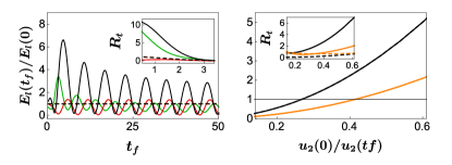
The initial state chosen for the numerical examples is a product of the ground state of the transversal harmonic oscillator and a minimum-uncertainty-product Gaussian in the longitudinal direction centered at $q_{l0}$, with initial momentum $p_{l0}$, $\psi_{l}(q_{l},t=0)={[\sigma\sqrt{2\pi}]^{-1/2}}\,\,\,e^{i\,p_{l0}\,q_{l}}e^{-{(q_{l}-q_{l0})^{2}}/{(4\,\sigma^{2})}}.$ Firstly, we design a process that interchanges $\omega_{1}(t)$ and $\omega_{2}(t)$ with $\Delta\theta=\pi/4$ and constant $\gamma$, conceived to preserve the initial longitudinal velocities in the outgoing waveguide, $E_{l}(t_{f})=E_{l}(0)$, and use linear ramps for the same boundary waveguides as a benchmark to compare the performance of the invariant-based protocol.

Figure 1a depicts the final longitudinal energy. For the linear ramps it oscillates with operation time. The envelope for the minima is at zero but the maximum tends for long times to some value that depends on the initial wave packet. Contrast this with the full stability of the invariant-lead processes. They guarantee a fixed result, the final longitudinal energy being identical to the initial one for any initial wave packet. The transversal excitation by the linear ramps in fast processes increases considerably as the initial wave packet deviates from the origin, while the transversal excitation in the invariant-based protocol is, in general, small and much more stable. It could be further suppressed by transverse focusing and/or optimizing the $u_{i}(t)$.

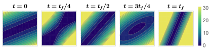
Figure 1b verifies that, for some chosen deflection angle, we can scale the final longitudinal energy at will in both scenarios ($\gamma$ or $\omega_{2}$ constant). Since the invariant does not affect the transversal direction, the transversal energy may be excited, but it depends on the design of the $u_{i}(t)$ so it can be minimized or even suppressed. Figure 2 provides snapshots of the evolution of the 2D potential for a $\omega_{2}$-constant processes that slows down the particle by a factor of two with deflection $\Delta\theta=\pi/4$.

State transfer. Up to now we have considered real $u_{j}(t)$, but the coupled Newton’s equations admit purely real and purely imaginary solutions combined into complex solutions. Exploiting this complex structure, $u_{i}=u_{i}^{R}+iu_{i}^{I}$, leads to interesting forms of the invariant. In particular the invariant may become proportional to the uncoupled Hamiltonians at boundary times. Let us first drop the waveguide condition (8) and go back to the laboratory frame variables $\{q_{1},q_{2}\}$. Defining annihilation operators in the usual manner, $a_{i}(t)=\sqrt{{\omega_{i}(t)}/{2}}\,q_{i}+{ip_{i}}/{\sqrt{2\omega_{i}(t)}},\,\;i=1,2,$ $G$ in Eq. (6) may become $a_{1}$ or $a_{2}$ by certain choices of the $u_{j}$. Let us choose at initial time

$$u_{1}(0)={ic_{0}}/{\sqrt{2\omega_{1}(0)}},\;\dot{u}_{1}(0)=-c_{0}\sqrt{{\omega_{1}(0)}/{2}},$$ (12)

and $u_{2}(0)=\dot{u}_{2}(0)=0$ with $c_{0}$ real. This implies $G(0)=c_{0}a_{1}(0)$, and $I(0)={c_{0}^{2}}a_{1}^{\dagger}(0)a_{1}(0)/2$. Instead, at final time we impose

$$u_{2}(t_{f})=ic_{0}/\sqrt{2\omega_{2}(t_{f})},\;\dot{u}_{2}(t_{f})=-c_{0}\sqrt{\omega_{2}(t_{f})/2},$$ (13)

together with $u_{1}(t_{f})=\dot{u}_{1}(t_{f})=0$, so that $G(t_{f})=c_{0}a_{2}(t_{f})$, and $I(t_{f})={c_{0}^{2}}a_{2}^{\dagger}(t_{f})a_{2}(t_{f})/2$. The same constant $c_{0}$ appears in Eqs. (12) and (13) because the solutions of Eq. (7) must satisfy $\frac{d}{dt}\{{\rm Im}[u_{1}^{*}(t)\dot{u}_{1}(t)+{u_{2}^{*}}(t)\dot{u}_{2}(t)]\}=0$ Thylwe1998 . The choice $c_{0}^{2}/2=\omega_{1}(0)$ gives $I(0)=H_{1}(0)$ and $I(t_{f})=[\omega_{1}(0)/\omega_{2}(t_{f})]H_{2}(t_{f})$, where we define the “uncoupled Hamiltonians” $H_{j}(t)\equiv\omega_{j}(t)a_{j}^{\dagger}(t)a_{j}(t)$. Eigenstates of $H_{1}(0)$ may thus be mapped into eigenstates of $H_{2}(t_{f})$ by proper inverse engineering of the $u_{j}(t)$. If $\omega_{1}(0)=\omega_{2}(t_{f})$,

$$\langle H_{1}(0)\rangle=\langle I(0)\rangle=\langle I(t_{f})\rangle=\langle H_{2}(t_{f})\rangle$$ (14)

for all initial wavepackets. (Any other scale factor may be chosen.) The system (7), which now involves four real functions, $u_{1}^{R}(t),u_{1}^{I}(t),u_{2}^{R}(t),u_{2}^{I}(t)$, has to be solved inversely for $\omega_{1}(t),\omega_{2}(t)$ and $\gamma(t)$. The inversion is done following techniques developed for trapped ions Palmero2017 or mechanical systems Gonzalez-Resines2017 , see appendices for a detailed account.

Figure 3: Upper: Control parameters, $\omega_{1}^{2}$ (dashed black), $\omega_{2}^{2}$ (short-dashed green) and $\gamma$ (solid blue) vs. $t/t_{f}$, for an energy transfer from oscillator 1 to 2. Lower: $\langle H_{1}\rangle$ in solid red, $\langle H_{2}\rangle$ in dashed blue, $\langle H\rangle$ in short-dashed green, and $\langle I\rangle$ in long-dashed black, for initial (left) and final (right) parts of the process. $\omega_{1}(0)^{2}=\omega_{2}(t_{f})^{2}=1$, $\omega_{2}(0)^{2}=\omega_{1}(t_{f})^{2}=0.9$ and $\gamma(0)=\gamma(t_{f})=6$; $t_{f}=4$; the system starts in a product state between the ground states of the uncoupled oscillators $H_{1}$ and $H_{2}$, not an eigenstate of the total Hamiltonian (1).

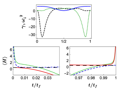
Figure (3)a displays the resulting evolution of the control parameters for a specific example in which the frequencies $\omega_{i}$ swap their boundary values and $\gamma(0)=\gamma(t_{f})$. Figure (3)b shows the expectation values of the total and the uncoupled Hamiltonians near the time boundaries, together with the constant expectation value of the invariant. Indeed $\langle H_{2}(t_{f})\rangle=\langle H_{1}(0)\rangle$.

Discussion. In some multidimensional systems with time-dependent control there are no point transformations that lead to uncoupled normal modes. Our main point here is that in these “coupled systems”, invariants of motion may still guide us to inversely design the time dependence of the controls for driving specific dynamics.

This inversion procedure extends the domain of invariant-based engineering, which had been applied so far to one dimensional or uncoupled systems Guery2019 . An important difference with respect to uncoupled systems is the diminished role of commutativity of Hamiltonian and invariant at boundary times. Commutativity, because of degeneracy, does not guarantee one-to-one mapping of eigenstates of the total Hamiltonian from initial to final configurations (see appendices). One should then focus on the invariant itself for applications, and, if required, rely on design freedom to keep other variables -e.g. the total energy- controlled. An alternative to be explored is to make use of a second invariant corresponding to a linearly independent set of classical solutions of Eq. (7), $\{u_{1}^{\prime}(t),u_{2}^{\prime}(t)\}$, linearly independent with respect to $\{u_{1}(t),u_{2}(t)\}$ Thylwe1998 . Imposing boundary conditions to the second set we would aim to control the second invariant as well, but the inversion problem becomes more demanding, as the number of conditions double while the number of (common) controls remains the same.

As for further open questions, invariant-based engineering is known to be related to other STA approaches such as counterdiabatic driving for single oscillators Chen2011_062116 . It would be of interest to connect the current work with CD driving for coupled oscillators Duncan2018 ; Villazon2019 . Finally, other boundary conditions on the $u_{j}$, see some examples in appendices, would allow to control other processes, different from the ones examined here.

Appendix B A: Commutation of Hamiltonian and invariant at boundary times

The eigenvectors of $I(t_{b})$ in the waveguide deflection example are highly degenerate, since a longitudinal plane wave multiplied by an arbitrary function of $q_{t}$ is a valid eigenvector with the same eigenvalue. This means that even if $I(t_{b})$ commutes with $H(t_{b})$ and shares some eigenvectors with $H(t_{b})$ the vast majority of them are not eigenvectors of $H(t_{b})$. This phenomenon -i.e., the existence of eigenvectors of one operator not shared with the other one- is well known but, since it sets an important difference with previous applications of invariant-based inverse engineering, we shall review briefly a few relevant aspects.

Let us consider a generic observable $A$ and an orthonormal set of eigenvectors of $A$ that forms a basis in the state space,

$$A|\phi_{n}^{i}\rangle=a_{n}|\phi_{n}^{i}\rangle;\hskip 28.45274pt\langle\phi_{n}^{i}|\phi_{n^{\prime}}^{i^{\prime}}\rangle=\delta_{n,n^{\prime}}\delta_{i,i^{\prime}},$$ (B.1)

where $i=1,2...g_{n}$ is the index to distinguish the eigenstates in the degenerate subspace for eigenvalue $a_{n}$, and $g_{n}$ is the degree of degeneracy of $a_{n}$. Now let us introduce an operator $B$ that commutes with $A$. Since $\langle\psi_{1}|B|\psi_{2}\rangle=0$ for any two eigenstates of $A$, $|\psi_{1}\rangle$ and $|\psi_{2}\rangle$, with different eigenvalues, we find a block-diagonal matrix for $B$ in the $\{|\phi_{n}^{i}\rangle\}$ basis, with blocks of dimension $g_{n}$ for each eigenvalue, where any element within each block can be nonzero Cohen-Tannoudji1991 .

If $g_{n}=1$ for all $n$, that is, all the eigenvalues are non-degenerate, the matrix is diagonal as all the blocks reduce to numbers $1\times 1$, and therefore the elements of the basis $\{|\phi_{n}^{i}\rangle\}$ are eigenvectors of $B$. This applies in virtually all previous works on invariant-based shortcuts in 1D Chen2010a ; Torrontegui2011 ; Tobalina2017 , in which the Hamiltonian and the invariant commute at initial and final time and are not degenerate, so they share the same eigenvectors at boundary times. Thus the inversely engineered protocol drives an eigenstate of the invariant from an eigenstate of the initial Hamiltonian $H(0)$ to an eigenstate of the final Hamiltonian $H(t_{f})$.

If $g_{n}>1$ for some $n$, the corresponding block does not reduce to a number and it is not, in general, diagonal. Thus, the elements of $\{|u_{n}^{i}\rangle\}$ are not, in general, eigenvectors of $B$. The consequence for inverse engineering applications is that, if $I(t)$ is an invariant and $H(t)$ the Hamiltonian, an initial eigenvector of both $I(0)$ and $H(0)$ is guaranteed to be dynamically mapped at final time into an eigenvector of $I(t_{b})$, but there is no guarantee that it will be simultaneously an eigenvector of $H(t_{b})$.

In particular, in the waveguide deflection example, the longitudinal energy may be conserved “asymptotically” at the time boundaries, but the process does not necessarily conserve the total energy. A factorized initial state with some longitudinal state multiplied by the transversal ground state will have at final time the same longitudinal energy that it had initially, in a different direction, but it can be transversally excited. Avoiding only longitudinal excitations is of interest per se, but we may make use of the flexibility of the shortcut design to minimize transversal excitation as well. Similarly, in the state-transfer example the energy of oscillator 1 is transferred to oscillator 2, but oscillator 1 could be excited.

In summary, commutativity of $H(t_{b})$ and $I(t_{b})$ plays a lesser role in the 2D scenario, and may in fact be abandoned for different applications. In particular $H(t_{b})$ and $I(t_{b})$ do not commute in the state-transfer example. The following section (B) explores alternative boundary conditions for the $u_{j}(t_{b})$ that imply different meanings for the invariant at the boundary times, and therefore different possible controlled processes.

Appendix C B: Other boundary conditions.

As the commutation of $I(t_{b})$ with $H(t_{b})$ does not guarantee the mapping among initial and final eigenstates of $H(t_{b})$, we shall drop this condition and explore other boundary conditions and forms of the invariant $I(t_{b})$.

For example, keeping the waveguide condition $\gamma(t_{b})=\omega_{1}(t_{b})\omega_{2}(t_{b})$, note the following alternative sets of boundary conditions and corresponding quadratic invariants:

$$\dot{u}_{i}(t_{b}) = 0,u_{1}(t_{b})\omega_{2}(t_{b})=-u_{2}(t_{b})\omega_{1}(t_{b}),$$

$$I(t_{b}) = \frac{u_{2}^{2}(t_{b})}{\cos^{2}\theta(t_{b})}\frac{p_{t}^{2}}{2},$$ (C.1)

where $i=1,2$ and the invariant at the boundary time $t_{b}$ is proportional to the transversal kinetic energy. As well,

$${u}_{i}(t_{b}) = 0,\;\dot{u}_{1}(t_{b})\omega_{1}(t_{b})=\dot{u}_{2}(t_{b})\omega_{2}(t_{b}),$$

$$I(t_{b}) = \frac{\dot{u}_{2}^{2}(t_{b})}{\sin^{2}\theta(t_{b})}\frac{q_{l}^{2}}{2};$$ (C.2)

or

$${u}_{i}(t_{b}) = 0,\;\dot{u}_{1}(t_{b})\omega_{2}(t_{b})=-\dot{u}_{2}(t_{b})\omega_{1}(t_{b}),$$

$$I(t_{b}) = \frac{\dot{u}_{2}^{2}(t_{b})}{\cos^{2}\theta(t_{b})}\frac{q_{t}^{2}}{2},$$ (C.3)

where the invariant at the boundary is proportional to the transversal potential energy.

The boundary conditions imposed on the $u_{i}(t)$ and their derivatives do not need to be of the same type at $t=0$ and $t_{f}$. Designing $u_{i}(t)$ so as to satisfy at $t=0$ and $t_{f}$ different boundary conditions opens several control possibilities such as, for example, driving the initial longitudinal energy into final transversal kinetic energy or viceversa.

Appendix D C: Uncoupled limit (waveguide with no deflection)

In the main text the time-dependent guiding from an incoming to an outgoing waveguide implies formally time-dependent coupled oscillators. If no deflection is desired, i.e. for $\Delta\theta=0$, the easiest approach is to keep the angle $\theta$ constant and the oscillators uncoupled, $\gamma=0$. We may thus identify $q_{l}=q_{1}$ and $q_{t}=q_{2}$, and the dynamics is separable into independent dynamical normal modes. There are linear invariants for each orthogonal direction, $G_{i}(t)=u_{i}(t)p_{i}-\dot{u}_{i}(t)q_{i}$, and corresponding quadratic invariants $I_{i}(t)=G_{i}^{\dagger}(t)G_{i}(t)/2$. Focusing on the longitudinal direction, by imposing the boundary conditions

$$\omega_{1}(t_{b}) = 0,$$

$$\dot{u}_{1}(t_{b}) = 0,$$ (D.1)

$G_{1}(t_{b})=u_{1}(t_{b})p_{1}$ is proportional to the longitudinal momentum. Consequences and applications, e.g. for cooling, are worked out in Muga2020 .

The transversal direction evolves independently. The simplest possibility is a waveguide with $\omega_{2}$ constant. Of course, compressions and or expansions may as well be designed for $\omega_{2}(t_{f})\neq\omega_{2}(0)$ via invariants, free from any transversal excitation as is well known Chen2010_063002 . In the current formal framework, making use of complex solutions as in the main text we would impose

$$u_{2}(0) = \frac{ic_{0}}{\sqrt{2\omega_{2}(0)}},\;\;\;\,\dot{u}_{2}(0)=-c_{0}\sqrt{\frac{\omega_{2}(0)}{{2}}},$$

$$u_{2}(t_{f}) = \frac{ic_{0}}{\sqrt{2\omega_{2}(t_{f})}},\;\dot{u}_{2}(t_{f})=-c_{0}\sqrt{\frac{\omega_{2}(t_{f})}{{2}}},$$ (D.2)

with $c_{0}$ real. This choice of boundary conditions implies

$$G_{2}(0) = c_{0}a_{2}(0),$$

$$I_{2}(0) = \frac{1}{2}G_{2}^{\dagger}(0)G_{2}(0)=\frac{c_{0}^{2}}{2}a_{2}^{\dagger}(0)a_{2}(0),$$ (D.3)

and at final time

$$G_{2}(t_{f}) = c_{0}a_{2}(t_{f}),$$

$$I_{2}(t_{f}) = \frac{1}{2}G^{\dagger}(t_{f})G(t_{f})=\frac{c_{0}^{2}}{2}a_{2}^{\dagger}(t_{f})a_{2}(t_{f}).$$ (D.4)

Choosing $c_{0}^{2}/2=\omega_{2}(0)$ gives $I_{2}(0)=H_{2}(0)$ and $I_{2}(t_{f})=\frac{\omega_{2}(0)}{\omega_{2}(t_{f})}H_{2}(t_{f})$, where $H_{2}(t)=\omega_{2}(t)a_{2}^{\dagger}(t)a(t)$. Eigenstates of $H_{2}(0)$ may thus be mapped into eigenstates of $H_{2}(t_{f})$ by proper inverse engineering of $u_{2}(t)$. The uncoupled equation for the transverse oscillator 2 in Eq. (7) which now involves two real functions, $u_{2}^{R}(t),u_{2}^{I}(t)$, has to be solved inversely for $\omega_{2}(t)$.

This approach is equivalent to the usual one using the Ermakov equation Chen2010_063002 . By writing $u_{2}(t)$ in polar form, $u_{2}(t)=\rho_{2}(t)e^{i\phi_{2}(t)}$, the harmonic oscillator equation splits into two coupled equations. One of them gives $\rho_{2}^{2}(t)\dot{\phi}_{2}=K$, with $K$ constant, and the other one is the Ermakov equation for $\rho_{2}(t)$ Thylwe1998 ; Guasti2002 ; Guasti2003 ,

$$\ddot{\rho}_{2}+\omega_{2}^{2}(t)\rho_{2}=\frac{K^{2}}{\rho_{2}^{3}}.$$ (D.5)

The invariant $I_{2}(t)$ becomes

$$I_{2} = I_{LR}-\frac{K}{2},$$

$$I_{LR} = \frac{1}{2}\left[\left(\frac{Kq_{2}}{\rho_{2}}\right)^{2}+\left(\rho_{2}p_{2}-\dot{\rho}_{2}q_{2}\right)^{2}\right],$$ (D.6)

where $I_{LR}$ is the “Lewis-Riesenfeld” invariant Lewis1969 . With the usual choice $K=\omega_{2}(0)$, and boundary conditions

$$\rho_{2}(0) = 1,\,\dot{\rho}_{2}(0)=\ddot{\rho}_{2}(0)=0,$$

$$\rho_{2}(t_{f}) = \left(\frac{\omega_{2}(0)}{\omega_{2}(t_{f})}\right)^{1/2},\,\dot{\rho}_{2}(t_{f})=\ddot{\rho}_{2}(t_{f})=0,$$ (D.7)

which are equivalent to Eq. (D.2) for $c_{0}=[2\omega_{2}(0)]^{1/2}$, $I_{LR}(0)=\omega_{2}(0)[a_{2}^{\dagger}(0)a_{2}(0)+1/2]$, whereas $I_{LR}(t_{f})=\omega_{2}(0)[a_{2}^{\dagger}(t_{f})a_{2}(t_{f})+1/2]$.

Appendix E D: Inverse engineering of a state transfer

Here we present the details of the inverse engineering for the state transfer protocol, we follow a method similar to the ones in refs. Palmero2017 ; Gonzalez-Resines2017 . Assuming that the values of the control parameters at boundary times are set, we start by designing a $\gamma(t)$ that satisfies the boundary values $\gamma(t_{b})$ and that has zero first and second derivatives at the boundaries for smoothness. We use a sum of cosines ansatz,

$$\gamma(t)=\sum_{k=0}^{4}a_{k}\cos\left(\frac{k\,\pi t}{t_{f}}\right),$$ (E.1)

which meets the boundary conditions with just five terms. The coefficient $a_{4}$ is left free for now. Then we design the imaginary part of the dynamics, again using sums of cosines,

$$u_{1}^{I}(t)=\sum_{i=0}^{6}b_{i}\cos\left(\frac{i\,\pi\,t}{t_{f}}\right),$$

$$u_{2}^{I}(t)=\sum_{j=0}^{6}c_{j}\cos\left(\frac{j\,\pi\,t}{t_{f}}\right).$$ (E.2)

Coefficients $\{b,c\}_{1-5}$ are fixed so that the real reference trajectories satisfy the boundary conditions for $u_{1,2}(t_{b})$ and its derivatives, and so that the frequencies $\omega_{i}(t)$ have the desired boundary values, which amounts to satisfying

$$\ddot{u} {}_{1}^{I}(0)=-\omega_{1}(0)^{2},\hskip 14.22636pt\ddot{u}_{1}^{I}(t_{f})=\gamma(t_{f})\sqrt{\frac{\omega_{1}(0)}{\omega_{2}(t_{f})}},$$ (E.3)

$$\ddot{u} {}_{2}^{I}(0)=\gamma(0),\hskip 8.5359pt\ddot{u}_{2}^{I}(t_{f})=\omega_{2}(tf)\sqrt{\omega_{1}(0)\omega_{2}(t_{f})}.$$

Note, from the expression of the frequencies

$$\omega_{1,2}(t)^{2}=\frac{\gamma(t)u_{2,1}^{I}(t)-\ddot{u}_{1,2}^{I}(t)}{u_{1,2}^{I}(t)},$$ (E.4)

that, even if the conditions in Eq. (E.3) are fulfilled, we may encounter indeterminacies at boundary times (some $u_{1,2}(t_{b})$ become $0$). Thus, we have to impose additional boundary conditions for consistency using L’Hopital’s rule,

$$u_{1}^{I\,(3)}(t_{f}) = 0,$$

$$u_{1}^{I\,(4)}(t_{f}) = -\gamma(t_{f})\sqrt{\frac{\omega_{1}(0)}{\omega_{2}(t_{f})}}\left[\omega_{1}(t_{f})^{2}+\omega_{2}(t_{f})^{2}\right],$$

$$u_{2}^{I\,(3)}(0) = 0,$$

$$u_{2}^{I\,(4)}(0) = -\gamma(0)\left[\omega_{1}(0)^{2}+\omega_{2}(0)^{2}\right].$$ (E.5)

Coefficients $\{b,c\}_{6}$ are left yet undetermined. In the next step, we numerically solve the real equations of motion with the already designed control parameters for the initial conditions and find with an optimization subroutine the value of the coefficients that have been left free to satisfy the final boundary conditions. For the specific example presented in the main text the “free” coefficients take the values $a_{4}=-0.659$, $b_{6}=-0.383$ and $c_{6}=-0.383$.

References

- (1) D. Kielpinski, C. Monroe, and D. J. Wineland, “Architecture for a large-scale ion-trap quantum computer.”, Nature 417, 709–11 (2002).
- (2) E. Torrontegui, S. Ibáñez, S. Martínez-Garaot, M. Modugno, A. del Campo, D. Guéry-Odelin, A. Ruschhaupt, X. Chen, and J. G. Muga, Shortcuts to Adiabaticity, volume 62 of Advances In Atomic, Molecular, and Optical Physics. Elsevier, 2013.
- (3) D. Guéry-Odelin, A. Ruschhaupt, A. Kiely, E. Torrontegui, S. Martí nez Garaot, and J. G. Muga, “Shortcuts to adiabaticity: concepts, methods, and applications”, preprint arXiv:1904.08448v1 (2019).
- (4) X. Chen, A. Ruschhaupt, S. Schmidt, A. del Campo, D. Guéry-Odelin, and J. G. Muga, “Fast Optimal Frictionless Atom Cooling in Harmonic Traps: Shortcut to Adiabaticity”, Physical Review Letters 104, 063002 (2010).
- (5) M. Demirplak and S. A. Rice, “Adiabatic Population Transfer with Control Fields”, The Journal of Physical Chemistry A 107, 9937–9945 (2003).
- (6) H. R. Lewis and P. G. L. Leach, “A direct approach to finding exact invariants for one-dimensional time-dependent classical Hamiltonians”, Journal of Mathematical Physics 23, 2371 (1982).
- (7) H. R. Lewis and W. B. Riesenfeld, “An Exact Quantum Theory of the Time-Dependent Harmonic Oscillator and of a Charged Particle in a Time-Dependent Electromagnetic Field”, Journal of Mathematical Physics 10, 1458 (1969).
- (8) A. Ruschhaupt, X. Chen, D. Alonso, and J. G. Muga, “Optimally robust shortcuts to population inversion in two-level quantum systems”, New Journal of Physics 14, 093040 (2012).
- (9) M. Palmero, R. Bowler, J. P. Gaebler, D. Leibfried, and J. G. Muga, “Fast transport of mixed-species ion chains within a Paul trap”, Physical Review A 90, 053408 (2014).
- (10) M. Palmero, S. Martínez-Garaot, J. Alonso, J. P. Home, and J. G. Muga, “Fast expansions and compressions of trapped-ion chains”, Physical Review A 91, 053411 (2015).
- (11) A. R. Urzúa, I. Ramos-Prieto, M. Fernández-Guasti, and H. M. Moya-Cessa, “Solution to the Time-Dependent Coupled Harmonic Oscillators Hamiltonian with Arbitrary Interactions”, Quantum Reports 1, 82–90 (2019).
- (12) I. Lizuain, M. Palmero, and J. G. Muga, “Dynamical normal modes for time-dependent Hamiltonians in two dimensions”, Phys. Rev. A 95, 022130 (2017).
- (13) M. Palmero, S. Martínez-Garaot, U. G. Poschinger, A. Ruschhaupt, and J. G. Muga, “Fast separation of two trapped ions”, New Journal of Physics 17, 093031 (2015).
- (14) M. Palmero, S. Martínez-Garaot, D. Leibfried, D. J. Wineland, and J. G. Muga, “Fast phase gates with trapped ions”, Physical Review A 95, 022328 (2017).
- (15) T. Sägesser, R. Matt, R. Oswald, and J. P. Home, “Fast dynamical exchange cooling with trapped ions”, 2020.
- (16) I. Lizuain, A. Tobalina, A. Rodriguez-Prieto, and J. G. Muga, “Fast state and trap rotation of a particle in an anisotropic potential”, Journal of Physics A: Mathematical and Theoretical 52, 465301 (2019).
- (17) R. Barends, J. Kelly, A. Megrant, D. Sank, E. Jeffrey, Y. Chen, Y. Yin, B. Chiaro, J. Mutus, C. Neill, P. O’Malley, P. Roushan, J. Wenner, T. C. White, A. N. Cleland, and J. M. Martinis, “Coherent Josephson Qubit Suitable for Scalable Quantum Integrated Circuits”, Phys. Rev. Lett. 111, 080502 (2013).
- (18) M. A. Rol, F. Battistel, F. K. Malinowski, C. C. Bultink, B. M. Tarasinski, R. Vollmer, N. Haider, N. Muthusubramanian, A. Bruno, B. M. Terhal, and L. DiCarlo, “Fast, High-Fidelity Conditional-Phase Gate Exploiting Leakage Interference in Weakly Anharmonic Superconducting Qubits”, Phys. Rev. Lett. 123, 120502 (2019).
- (19) B. Peropadre, D. Zueco, F. Wulschner, F. Deppe, A. Marx, R. Gross, and J. J. García-Ripoll, “Tunable coupling engineering between superconducting resonators: From sidebands to effective gauge fields”, Phys. Rev. B 87, 134504 (2013).
- (20) J. J. García-Ripoll, A. Ruiz-Chamorro, and E. Torrontegui, “Quantum control of transmon superconducting qubits”, arXiv:2002.10320 [quant-ph].
- (21) Y. Chen, C. Neill, P. Roushan, N. Leung, M. Fang, R. Barends, J. Kelly, B. Campbell, Z. Chen, B. Chiaro, A. Dunsworth, E. Jeffrey, A. Megrant, J. Y. Mutus, P. J. J. O’Malley, C. M. Quintana, D. Sank, A. Vainsencher, J. Wenner, T. C. White, M. R. Geller, A. N. Cleland, and J. M. Martinis, “Qubit Architecture with High Coherence and Fast Tunable Coupling”, Phys. Rev. Lett. 113, 220502 (2014).
- (22) D. Kleckner, B. Pepper, E. Jeffrey, P. Sonin, S. M. Thon, and D. Bouwmeester, “Optomechanical trampoline resonators”, Opt. Express 19, 19708–19716 (2011).
- (23) K. Zhang, F. Bariani, and P. Meystre, “Quantum Optomechanical Heat Engine”, Phys. Rev. Lett. 112, 150602 (2014).
- (24) M. Aspelmeyer, T. J. Kippenberg, and F. Marquardt, “Cavity optomechanics”, Rev. Mod. Phys. 86, 1391–1452 (2014).
- (25) H. Goldstein, C. Poole, and J. Safko, “Classical mechanics”, 2002.
- (26) M. Fernández-Guasti and A. Gil-Villegas, “Orthogonal functions invariant for the time-dependent harmonic oscillator”, Physics Letters A 292, 243 - 245 (2002).
- (27) M. Fernández-Guasti and H. Moya-Cessa, “Solution of the Schrödinger equation for time-dependent 1D harmonic oscillators using the orthogonal functions invariant”, Journal of Physics A 36, 2069–2076 (2003).
- (28) K.-E. Thylwe and H. J. Korsch, “The `Ermakov - Lewis' invariants for coupled linear oscillators”, Journal of Physics A 31, L279–L285 (1998).
- (29) O. Castanos, R. Lopez-Pena, and V. I. Man'ko, “Noether's theorem and time-dependent quantum invariants”, Journal of Physics A 27, 1751–1770 (1994).
- (30) V. I. Arnold, Mathematical Methods of Classical Mechanics, 2nd ed. Springer-Verlag, 1989.
- (31) S. González-Resines, D. Guéry-Odelin, A. Tobalina, I. Lizuain, E. Torrontegui, and J. G. Muga, “Invariant-Based Inverse Engineering of Crane Control Parameters”, Phys. Rev. Applied 8, 054008 (2017).
- (32) X. Chen, E. Torrontegui, and J. G. Muga, “Lewis-Riesenfeld invariants and transitionless quantum driving”, Phys. Rev. A 83, 062116 (2011).
- (33) C. W. Duncan and A. del Campo, “Shortcuts to adiabaticity assisted by counterdiabatic Born–Oppenheimer dynamics”, New Journal of Physics 20, 085003 (2018).
- (34) T. Villazon, A. Polkovnikov, and A. Chandran, “Swift heat transfer by fast-forward driving in open quantum systems”, Phys. Rev. A 100, 012126 (2019).
- (35) C. Cohen-Tannoudji, B. Diu, and F. Laloe, Quantum Mechanics. Wiley, 1991.
- (36) X. Chen, A. Ruschhaupt, S. Schmidt, A. del Campo, D. Guéry-Odelin, and J. G. Muga, “Fast Optimal Frictionless Atom Cooling in Harmonic Traps: Shortcut to Adiabaticity”, Physical Review Letters 104, 063002 (2010).
- (37) E. Torrontegui, S. Ibáñez, X. Chen, A. Ruschhaupt, D. Guéry-Odelin, and J. G. Muga, “Fast atomic transport without vibrational heating”, Physical Review A 83, 013415 (2011).
- (38) A. Tobalina, M. Palmero, S. Martínez-Garaot, and J. G. Muga, “Fast atom transport and launching in a nonrigid trap”, Scientific Reports 7, 5753 (2017).
- (39) J. G. Muga, S. Martínez-Garaot, M. Pons, M. Palmero, and A. Tobalina, “Time-dependent harmonic potentials for momentum or position scaling”, arXiv preprint arXiv:2007.09949 (2020).