A new framework for the computation of Hessians

Abstract

We investigate the computation of Hessian matrices via Automatic Differentiation, using a graph model and an algebraic model. The graph model reveals the inherent symmetries involved in calculating the Hessian. The algebraic model, based on Griewank and Walther’s state transformations [16], synthesizes the calculation of the Hessian as a formula. These dual points of view, graphical and algebraic, lead to a new framework for Hessian computation. This is illustrated by developing edge_pushing, a new truly reverse Hessian computation algorithm that fully exploits the Hessian’s symmetry. Computational experiments compare the performance of edge_pushing on sixteen functions from the CUTE collection [6] against two algorithms available as drivers of the software ADOL-C [15, 23, 11], and the results are very promising.

1 Introduction

Within the context of nonlinear optimization, algorithms that use variants of Newton’s method must repeatedly calculate or obtain approximations of the Hessian matrix or Hessian-vector products. Interior-point methods, ubiquitous in nonlinear solvers [10], fall in this category. While the nonlinear optimization package LOQO [21] requires that the user supply the Hessian, IPOPT [22] and KNITRO [7] are more flexible, but also use Hessian information of some kind or other. Experience indicates that optimization algorithms that employ first order derivatives perform fewer iterations given exact gradients, as opposed to numerically approximated ones. Although there is not an equivalent consensus concerning second order derivatives, it is natural to suspect the same would hold true for algorithms that use Hessians. Thus the need to efficiently calculate exact (up to machine precision) Hessian matrices is driven by the rising popularity of optimization methods that take advantage of second-order information.

Automatic Differentiation (AD) has had a lot of success in calculating gradients and Hessian-vector products with reverse AD procedures [8] that have the same time complexity as that of evaluating the underlying function.

Attempts to efficiently calculate the entire Hessian matrix date back to the work of Jackson and McCormick [19], based on Jackson’s dissertation. Their work was followed by increasingly intense research in this area, no doubt helped along by the advances in hardware and software. Since the beginning, exploring sparsity and symmetry were at the forefront of efficiency related issues. Nowadays we can discern a variety of strategies in the literature, regarding how to properly take these into account. The authors of [19] explore sparsity and symmetry by storing and operating on the Hessian in an outer product format, the so called dyadic form. A natural strategy, when employing a forward Hessian mode, is to store the Hessian matrices involved in data structures that accommodate their symmetry [2]. When dealing with very sparse matrices, one may obtain the sparsity pattern, and then individually calculate selected nonzero elements using methods such as univariate Taylor expansion [2, 5]. Truly effective methods currently in use, with a substantial number of reports including numerical tests, take advantage of sparsity and symmetry by combining graph coloring with Hessian-vector AD routines [11, 23].

The paper is organized as follows. Section 2 presents concepts and notation regarding function and gradient evaluation in AD. The graph model for Hessian computation is developed in Section 3 and the algebraic formula for the Hessian is obtained in the next section. The new algorithm, edge_pushing, or e_p for short, is described in Section 5. The computational experiments are reported in Section 6 and we close with conclusions and comments on future work.

2 Preliminaries: function and gradient computation

In order to simplify the discussion, we consider functions $f\colon\mathbb{R}^{n}\to\mathbb{R}$ that are twice continuously differentiable. It is more convenient and the results obtained can be generalized in a straightforward manner to smaller domains and functions that are twice continuously differentiable by parts. There are of course multiple possibilities for expressing a function, but even if one chooses a specific way to write down a function, or a specific way of programming a function $f$, one still may come up with several distinct translations of $f$ into a finite sequential list of functions. We assume in the following that such a list has already been produced, namely there exists a sequence $(\phi_{1-n},\ldots,\phi_{0},\phi_{1},\ldots,\phi_{\ell})$, such that the first $n$ functions are the coordinate variables, each intermediate function $\phi_{i}$, for $i=1,\ldots,\ell$, is a function of previous functions in the sequence, and, if we sweep this sequence in a forward fashion, starting with some fixed vector $x=(\phi_{1-n},\ldots,\phi_{0})$, the value obtained for $\phi_{\ell}$ coincides with the value of $f(x)$. Jackson and McCormick [19] dealt with a very similar concept, which they called a factorable function, but in that case the intermediate functions were either sums or products of precisely two previous functions, or generic functions of a single previous function, that is, unary functions. Although the framework for calculating the Hessian developed here is valid for intermediate functions with any number of input variables, when evaluating complexity bounds, we assume that the functions $\phi_{i}$, for $i=1,\ldots,\ell$, are either unary or binary.

It is very convenient to model the sequential list $(\phi_{1-n},\ldots,\phi_{\ell})$ and the interdependence amongst its components as an acyclic digraph $G=(N,A)$, called computational graph. Loosely speaking, the computational graph associated with the list has nodes $\{1-n,\ldots,\ell\}$ and edges $\{(j,i)\mid\phi_{i}\mbox{ depends on the}$ $\mbox{value of }\phi_{j}\}$. The interdependence relations are thus translated into predecessor relations between nodes, and are denoted by the symbol $\prec$. Thus the arc $(j,i)$ embodies the precedence relation $j\prec i$. Notice that, by construction, $j\prec i$ implies $j<i$. Furthermore, if we denote by $v_{i}$ the output value of $\phi_{i}$ for a given input, then we may shorten, for instance, the expression $v_{i}=\phi_{i}(v_{j},v_{k})$ to $v_{i}=\phi_{i}(v_{j})_{j\prec i}$.

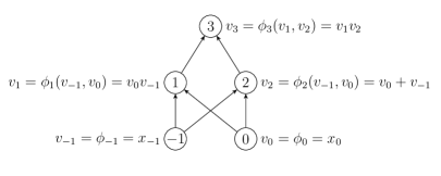
Figure 1: Computational graph of the function $f(x)=(x_{-1}x_{0})(x_{-1}+x_{0})$.

Due to the choice of the numbering scheme for the $\phi$’s, commonly adopted in the literature, we found it convenient to apply, throughout this article, a shift of $-n$ to the indices of all matrices and vectors. We already have $x\in\mathbb{R}^{n}$, which, according to this convention, has components $x_{1-n}$, $x_{2-n}$, …, $x_{0}$. Similarly, the rows/columns of the Hessian $f^{\prime\prime}$ are numbered $1-n$ through $0$. Other vectors and matrices will be gradually introduced, as the need arises for expressing and deducing mathematical properties enjoyed by the data. Figure 1 shows the computational graph of function $f(x)=(x_{-1}x_{0})(x_{-1}+x_{0})$ that corresponds to the sequence $(v_{-1},\ldots,v_{3})=(x_{-1},x_{0},x_{-1}x_{0},x_{-1}+x_{0},(x_{-1}x_{0})(x_{-1}+x_{0}))$.

Griewank and Walther’s [16] representation of $f$ as a composition of state transformations

$$f(x)=e_{\ell}^{T}(\Phi_{\ell}\circ\Phi_{\ell-1}\circ\cdots\circ\Phi_{1})(P^{T}x),$$ (1)

where $e_{\ell}$ is the $(\ell+n)$th canonical vector, the $n\times(n+\ell)$ matrix $P$ is zero except for the leftmost $n$-dimensional block which contains an identity matrix, and

$$\Phi_{i} \colon \mathbb{R}^{n+\ell}\to\mathbb{R}^{n+\ell}$$ (2)

$$\parbox{25.0pt}{\centerline{\hbox{$y$}}}\mapsto(y_{1-n},\ldots,y_{i-1},\phi_{i}(y_{j})_{j\prec i},y_{i+1},\ldots,y_{\ell})^{T}$$

leads to a synthetic formula for the gradient of $f$, using the chain rule recursively:

$$(\nabla f(x))^{T}=e_{\ell}^{T}\Phi_{\ell}^{\prime}\Phi_{\ell-1}^{\prime}\cdots\Phi_{1}^{\prime}P^{T}.$$ (3)

For simplicity’s sake, the argument of each function is omitted in (3), but it should be noted that $\Phi_{k}^{\prime}$ is evaluated at $(\Phi_{k-1}\circ\Phi_{k-2}\circ\cdots\circ\Phi_{1})(P^{T}x)$, for $k=1,\ldots,\ell$.

The advantage of vector/matrix notation is that formulas expressed in terms of vector/matrix operations usually lend themselves to straightforward algorithmic implementations. Nevertheless, when analyzing complexity issues and actual implementation, one has to translate block operations with vectors or matrices into componentwise operations on individual variables.

In this case, for instance, one can immediately devise two ways of obtaining $\nabla f$ based on (3): calculating the product of the matrices in a right-to-left fashion, or left-to-right. The latter approach constituted a breakthrough in gradient computation, since the time complexity of its implementation was basically the same as that of the function evaluation, a major improvement over the former approach. In the left-to-right way, the indices are traveled in decreasing order, so this method of calculating the gradient is called the reverse gradient computation. Notice that, in graph terms, this corresponds to a backward sweep of the computational graph.

Of course, one needs the values of $v_{j}$, for $j\prec i$, in order to calculate $v_{i}$. Thus in order to do perform a backward sweep, it must be preceded by a forward sweep, in which all the values $v_{i}$, for $i=1,\ldots,\ell$, have been calculated. We shall call the data structure that contains all information concerning the function evaluation produced during the forward sweep a tape $\mathcal{T}$. Thus the tape contains the relevant recordings of a forward sweep along with the computational graph of $f$.

Algorithms 1 and 2 contain the implementation of the reverse gradient computation in block and componentwise forms, respectively.

In Algorithm 1 the necessary partial products are stored in $\overline{\mathrm{v}}$, and, right before node $i$ is swept, the vector $\overline{\mathrm{v}}$ satisfies

$$\overline{\mathrm{v}}^{T}=e^{T}_{\ell}\prod_{j=1}^{\ell-i}\Phi^{\prime}_{\ell-j+1}.$$ (4)

The streamlined componentwise form of Algorithm 1 follows from the very simple block structure of the Jacobian $\Phi_{i}^{\prime}$:

$$\Phi_{i}^{\prime}=\left[\begin{array}[]{@{\hspace{7pt}}c@{\hspace{8pt}}|@{\hspace{5pt}}c@{\hspace{5pt}}|@{\hspace{11pt}}c@{\hspace{7pt}}}\hskip 7.0pt\lx@intercol\hfil\rule{0.0pt}{23.0pt}\rule[-13.0pt]{0.0pt}{10.0pt}I\hfil\hskip 8.0pt\vrule\hskip 5.0&0\hfil\hskip 5.0pt\vrule\hskip 11.0&0\makebox(0.0,10.0)[lc]{\footnotesize$\begin{array}[]{@{\hspace{.5cm}}c}\hskip 14.22636pt\lx@intercol\hfil 1-n\\[-5.0pt] \hskip 14.22636pt\lx@intercol\hfil\vdots\\[-3.0pt] \hskip 14.22636pt\lx@intercol\hfil i-1\end{array}$}\hfil\hskip 7.0\\ \hline\cr\hskip 7.0pt\lx@intercol\hfil(c^{i})^{T}\rule{0.0pt}{12.0pt}\hfil\hskip 8.0pt\vrule\hskip 5.0&0\hfil\hskip 5.0pt\vrule\hskip 11.0&0\makebox(0.0,10.0)[lc]{\footnotesize\hskip 14.22636ptrow$i$,}\hfil\hskip 7.0\\ \hline\cr\hskip 7.0pt\lx@intercol\hfil\rule{0.0pt}{23.0pt}\rule[-10.0pt]{0.0pt}{10.0pt}0\hfil\hskip 8.0pt\vrule\hskip 5.0&0\hfil\hskip 5.0pt\vrule\hskip 11.0&I\makebox(0.0,10.0)[lc]{\footnotesize$\begin{array}[]{@{\hspace{.5cm}}c}\hskip 14.22636pt\lx@intercol\hfil i+1\\[-5.0pt] \hskip 14.22636pt\lx@intercol\hfil\vdots\\[-3.0pt] \hskip 14.22636pt\lx@intercol\hfil\ell\end{array}$}\hfil\hskip 7.0\end{array}\right]$$ (5)

where

$$(c^{i})_{j}=\frac{\partial\phi_{i}}{\partial v_{j}},\quad\mbox{for }j=1-n,\ldots,i-1.$$ (6)

Thus $(c^{i})^{T}$ is basically the transposed gradient of $\phi_{i}$ padded with the convenient number of zeros at the appropriate places. In particular, it has at most as many nonzeros as the number of predecessors of node $i$, and the post-multiplication $\overline{\mathrm{v}}^{T}\Phi^{\prime}_{i}$ affects the components of $\overline{\mathrm{v}}$ associated with the predecessors of node $i$ and zeroes component $i$. In other words, denoting component $i$ of $\overline{\mathrm{v}}$ by $\bar{v}_{i}$, the block assignment in Algorithm 1 is equivalent to

$$\bar{v}_{j}\leftarrow\left\{\begin{array}[]{ll}\bar{v}_{j}+\bar{v}_{i}\dfrac{\partial\phi_{i}}{\partial v_{j}},&\mbox{if }j\prec i,\\ 0,&\mbox{if }j=i,\\[5.0pt] \bar{v}_{j},&\mbox{otherwise.}\end{array}\right.$$

Now this assignment is done as the node $i$ is swept, and, therefore, in subsequent iterations component $i$ of $\overline{\mathrm{v}}$ will not be accessed, since the loop visits nodes in decreasing index order. Hence setting component $i$ to zero has no effect on the following iterations. Eliminating this superfluous reduction, we arrive at Algorithm  2, the componentwise (slightly altered) version of Algorithm 1.

In order to give a graph interpretation of Algorithm 2, let $c^{i}_{j}=\partial\phi_{i}/\partial v_{j}$ be the weight of arc $(j,i)$, and define the weight of a directed path from node $j$ to node $k$ as the product of the weights of the arcs in the path. Then, one can easily check by induction that, right before node $i$ is swept, the adjoint $\bar{v}_{i}$ contains the sum of the weights of all the paths from node $i$ to node $\ell$:

$$\bar{v}_{i}=\sum_{p\mid\mbox{\scriptsize path from $i$ to $\ell$}}\mbox{weight of path }p,$$ (7)

and $\partial f/\partial v_{i}=\bar{v}_{i}$. This formula has been known for quite some time [3].

As node $i$ is swept, the value of $\bar{v}_{i}$ is properly distributed amongst its predecessors, in the sense that, accumulated in $\bar{v}_{j}$, for each predecessor $j$, is the contribution of all paths from $j$ to $\ell$ that contain node $i$, weighted by $c^{i}_{j}$. Hence, at the end of Algorithm 2, the adjoint $\bar{v}_{i-n}$, for $i=1,\ldots,n$, contains the sum of the weights of all paths from $i-n$ to $\ell$. This is in perfect accordance with the explanation for the computation of partial derivatives given in some Calculus textbooks, see, for instance, [20, p. 940].

Of course different ways of calculating the product of the Jacobians of the state transformations in (3) may give rise to different algorithms. In the following, using the same ingredients, we obtain a closed formula for the Hessian, that can be used to justify known algorithms as well as suggest a new algorithm for Hessian computation. Before that, however, we develop a graph understanding of the Hessian computation.

3 Hessian graph model

Creating a graph model for the Hessian is also very useful, as it provides insight and intuition regarding the workings of Hessian algorithms. Not only can the graph model suggest algorithms, it can also be very enlightening to interpret the operations performed by an algorithm as operations on variables associated with the nodes and arcs of a computational graph.

Since second order derivatives are simply first order derivatives of the gradient, a natural approach to their calculation would be to build a computational graph for the gradient and apply a variant of Algorithm 2 on this new graph to obtain the second order partial derivatives. We do this to better understand the problem, but later on we will see that it is not really necessary to build the full-fledged gradient computational graph, but one can instead work with the original graph plus some new edges.

Of course the gradient may be represented by distinct computational graphs, or equivalently, sequential lists of functions, but the natural one to consider is the one associated with the computation performed by Algorithm 2. Assuming this choice, the gradient $\nabla f=(\bar{v}_{1-n},\ldots,\bar{v}_{0})^{T}$ is a composite function of $(\bar{v}_{1},\ldots,\bar{v}_{\ell})$, as well as $(v_{1-n},\ldots,v_{\ell})$, which implies that the gradient (computational) graph $G^{g}=(N^{g},A^{g})$ must contain $G$. The graph $G^{g}$ is basically built upon $G$ by adding nodes associated with $\bar{v}_{i}$, for $i=1-n,\ldots,\ell$, and edges representing the functional dependencies between these nodes.

Thus the node set $N^{g}$ contains $2(n+\ell)$ nodes $\{1-n,\ldots,\ell,\overline{1-n},\ldots,\overline{\ell}\}$, the first half associated with the original variables and the second half with the adjoint variables. The arc set is $A^{g}=A_{1}\cup A_{2}\cup A_{3}$, where $A_{1}$ contains arcs with both endpoints in “original” nodes; $A_{2}$, arcs with both endpoints in “adjoint” nodes and $A_{3}$, arcs with endpoints of mixed nature. Since running Algorithm 2 does not introduce new dependencies amongst the original $v$’s, we have that $A_{1}=A$.

The new dependent variables created by running Algorithm 2 satisfy

$$\bar{v}_{i}=\sum_{k\mid i\prec k}\bar{v}_{k}\frac{\partial v_{k}}{\partial v_{i}}$$ (8)

at the end of the algorithm. Expression (8) indicates that $\bar{v}_{i}$ depends on $\bar{v}_{k}$ for every $k$ that is a successor of $i$. Thus every arc $(i,k)\in A_{1}$ gives rise to arc $(\bar{k},\overline{\textit{\i}})\in A_{2}$. Therefore arcs in $A_{2}$ are copies of the arcs in $A$ with the orientation reversed. The graph $G^{g}$ thus contains $G$ and a kind of a mirror copy of $G$. Furthermore, if a partial derivative $\partial v_{k}/\partial v_{i}$ in the sum in (8) is not constant, but is a function of some $v_{j}$, this gives rise to the precedence relation $j\prec\overline{\textit{\i}}$. Notice that this may only happen if $j\prec k$, that is, the arcs $(j,\overline{\textit{\i}})\in A_{3}$ imply that $j$ and $i$ share a common successor $k$. This implies, in particular, that there are no edges incident to $\overline{\ell}$.

Apparently, the computational graph of the gradient was first described in [9], but can be found in a number of places, e.g., [16, p. 237].

Figure 2 shows the computational graph of the gradient of the function $f$ given in Figure 1. Notice that on the left we have the computational graph of $f$ and, on the right, a mirror copy thereof. Arcs in $A_{3}$ are the ones drawn dashed in the picture.

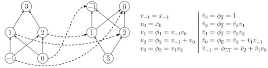
Figure 2: Gradient computational graph $G^{g}$ of the function $f(x)=(x_{-1}x_{0})(x_{-1}+x_{0})$, represented by the computational graph in Figure 1.

Mimicking (7), we conclude that

$$\frac{\partial^{2}f}{\partial x_{i}\partial x_{j}}=\sum_{p\mid\mbox{\scriptsize path from $i$ to $\overline{\textit{\j}}$}}\mbox{weight of path $p$}.$$ (9)

The weights of arcs $(i,j)\in A_{1}$ are already know. Equation (8) implies that the weight of arc $(\overline{\textit{\i}},\overline{\textit{\j}})\in A_{2}$ is

$$c^{\kern 1.0pt\overline{\textit{\j}}}_{\rule{0.0pt}{8.0pt}\overline{\textit{\i}}}=\frac{\partial v_{i}}{\partial v_{j}}=c^{i}_{j},$$ (10)

that is, arc $(i,j)$ has the same weight as its mirror image.

The weight of arc $(j,\textit{\i})$ is also obtained from (8)

$$c^{\overline{\textit{\i}}}_{j} = \sum_{k\mid i\prec k}\bar{v}_{k}\frac{\partial^{2}v_{k}}{\partial v_{j}\partial v_{i}}$$ (11)

$$= \sum_{k\mid i\prec k~{}\mbox{\scriptsize and}~{}j\prec k}\bar{v}_{k}\frac{\partial^{2}v_{k}}{\partial v_{j}\partial v_{i}},$$

since the partial derivative $\partial^{2}v_{k}/\partial v_{j}\partial v_{i}$ is identically zero if $k$ is not a successor of $j$. In particular, (11) and the fact that $f$ is twice continuously differentiable imply that

$$c^{\overline{\textit{\i}}}_{j}=c^{\overline{\textit{\j}}}_{\rule{0.0pt}{8.0pt}i},\mbox{ for }j\neq i.$$ (12)

Notice that arcs in $A_{3}$ are the only ones with second-order derivatives as weights. In a sense, they carry the nonlinearity of $f$, which suggests the denomination nonlinear arcs.

Regarding the paths in $G^{g}$ from $i$ to $\overline{\textit{\j}}$, for fixed $i,j\in\{1-n,\ldots,0\}$, each of them contains a unique nonlinear arc, since none of the original nodes is a successor of an adjoint node. Therefore, the sum in (9) may be partitioned according to the nonlinear arc utilized by the paths as follows:

$$\frac{\partial^{2}f}{\partial x_{i}\partial x_{j}}=\kern-9.0pt\sum_{(r,\overline{s})\in A_{3}}\!\!\left[\!\left(\sum_{p\mid\mbox{\scriptsize path from $i$ to $r$}}\kern-20.0pt\mbox{weight of path $p$}\right)c^{\overline{s}}_{r}\left(\sum_{q\mid\mbox{\scriptsize path from $\overline{s}$ to $\overline{\textit{\j}}$}}\kern-19.0pt\mbox{weight of path $q$}\right)\!\right]\!,$$ (13)

which reduces to

$$\frac{\partial^{2}f}{\partial x_{i}\partial x_{j}}=\kern-9.0pt\sum_{(r,\overline{s})\in A_{3}}\!\!\left[\!\left(\sum_{p\mid\mbox{\scriptsize path from $i$ to $r$}}\kern-20.0pt\mbox{weight of path $p$}\right)c^{\overline{s}}_{r}\left(\sum_{q\mid\mbox{\scriptsize path from $j$ to $s$}}\kern-19.0pt\mbox{weight of path $q$}\right)\!\right]\!,$$ (14)

where the second set of summations is replaced using the symmetry in (10).

On close examination, there is a lot of redundant information in $G^{g}$. One really doesn’t need the mirror copy of $G$, since the information attached to the adjoint nodes can be recorded associated to the original nodes and the arc weights of the mirror arcs are the same. Now if we fold back the mirror copy over the original, identifying nodes $k$ and $\overline{k}$, we obtain a graph with same node set as $G$ but with an enlarged set of arcs. Arcs in $A$ will be replaced by pairs of arcs in opposite directions and nonlinear arcs will become either loops (in case one had an arc $(i,\overline{\textit{\i}})$ in $A_{3}$) or pairs of arcs with opposite orientations between the same pair of nodes. Also, equations (10) and (12) imply that all arcs in parallel have the same weight, see Figure 3. This is still too much redundancy. We may leave arcs in $A$ as they are, replace the pairs of directed nonlinear arcs in opposite directions with a single undirected arc between the same pair of nodes and the directed loops by undirected ones, as exemplified in Figure 3, as long as we keep in mind the special characteristics of the paths we’re interested in.

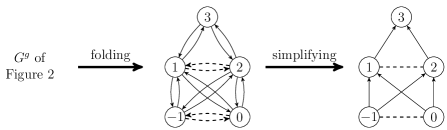
Figure 3: Folding of the gradient computational graph of Figure 2 and further elimination of redundancies.

The paths needed for the computation of the Hessian, in the folded and simplified graph, are divided into three parts. In the first part we have a directed path from some zero in-degree node, say $i$, to some other node, say $r$. Next comes an undirected nonlinear arc $(r,s)$. The last part is a path from $s$ to another zero in-degree node, say $j$, in which all arcs are traveled in the wrong direction. Of course, both the first and third parts of the path may be empty, only the middle part (the nonlinear arc) is mandatory.

This folded and simplified graph can be interpreted as a reduced gradient graph, with the symmetric redundancies removed. The graph together with the tri-parted path interpretation for partial derivatives constitutes our graph model for the Hessian. In Section 5 we will present an algorithm that takes full advantage of these symmetries and has a natural interpretation as an algorithm that gradually introduces nonlinear arcs and accumulates the weights of these special paths in the computational graph. In contrast, the authors in [4] build the entire gradient graph to then use an axial symmetry detection algorithm on this computational graph in order to eliminate redundancies. Once this is done, the Hessian is calculated via Jacobian methods.

4 Hessian formula

The closed formula to be developed concerns the Hessian of a function $g$ that is defined as a linear combination of the functions $\Psi_{1}$, …, $\Psi_{p}$, or, in matrix form,

$$g(x)=y^{T}\Psi(x),$$ (15)

where $y\in\mathbb{R}^{p}$ and $\Psi\in C^{2}(\mathbb{R}^{n},\mathbb{R}^{p})$. The linearity of the differential operator implies that the Hessian of $g$ is simply the linear combination of the Hessians of $\Psi_{1}$, …, $\Psi_{p}$:

$$g^{\prime\prime}(x)=\sum_{i=1}^{p}y_{i}\Psi^{\prime\prime}_{i}(x).$$ (16)

This motivates the introduction of the following definition of the vector-tensor product $y^{T}\Psi^{\prime\prime}(x)$, in order to establish an analogy between the linear combinations in (15) and (16):

$$g^{\prime\prime}(x)=(y^{T}\Psi(x))^{\prime\prime}=y^{T}\Psi^{\prime\prime}=\sum_{i=1}^{p}y_{i}\Psi^{\prime\prime}_{i}(x).$$ (17)

Next we need to establish how to express $g^{\prime\prime}$ when $\Psi$ is a composition of vector functions of several variables, the subject of the next Proposition.

Proposition 4.1.

Let $y\in\mathbb{R}^{p}$, $\Omega\in C^{2}(\mathbb{R}^{n},\mathbb{R}^{m})$, $\Theta\in C^{2}(\mathbb{R}^{m},\mathbb{R}^{p})$ and $\Psi(x)=\Theta\circ\Omega(x)$. Then

$$y^{T}\Psi^{\prime\prime}=(\Omega^{\prime})^{T}(y^{T}\Theta^{\prime\prime})\Omega^{\prime}+(y^{T}\Theta^{\prime})\Omega^{\prime\prime}.$$ (18)

Proof.

By definition, applying differentiation rules, and using the symmetry of the Hessian, we may calculate entry $(j,k)$ of the Hessian as follows:

$$(y^{T}\Psi^{\prime\prime}(x))_{jk} = \sum_{i}y_{i}\;\frac{\partial^{2}\Psi_{i}(x)}{\partial x_{j}\partial x_{k}}$$

$$= \sum_{i}y_{i}\;\frac{\partial}{\partial x_{j}}\left(\frac{\partial\Theta_{i}(\Omega(x))}{\partial x_{k}}\right)$$

$$= \sum_{i}y_{i}\;\frac{\partial}{\partial x_{j}}\left(\sum_{r=1}^{m}\frac{\partial\Theta_{i}(\Omega(x))}{\partial\Omega_{r}}\frac{\partial\Omega_{r}(x)}{\partial x_{k}}\right)$$

$$= \displaystyle\sum_{i}\sum_{r}y_{i}\left[\frac{\partial}{\partial x_{j}}\left(\frac{\partial\Theta_{i}(\Omega(x))}{\partial\Omega_{r}}\right)\right]\frac{\partial\Omega_{r}(x)}{\partial x_{k}}+\sum_{i}\sum_{r}y_{i}\;\frac{\partial\Theta_{i}(\Omega(x))}{\partial\Omega_{r}}\frac{\partial^{2}\Omega_{r}(x)}{\partial x_{j}\partial x_{k}}$$

$$= \sum_{r}\sum_{s}\sum_{i}y_{i}\;\frac{\partial^{2}\Theta_{i}(\Omega(x))}{\partial\Omega_{s}\partial\Omega_{r}}\frac{\partial\Omega_{s}(x)}{\partial x_{j}}\frac{\partial\Omega_{r}(x)}{\partial x_{k}}+\sum_{r}(y^{T}\Theta^{\prime}(\Omega(x))_{r}(\Omega^{\prime\prime}_{r}(x))_{jk}$$

$$= \sum_{s}\sum_{r}(y^{T}\Theta^{\prime\prime}(\Omega(x)))_{rs}\left(\Omega^{\prime}(x)\right)_{sj}\left(\Omega^{\prime}(x)\right)_{rk}+\sum_{r}(y^{T}\Theta^{\prime}(\Omega(x))_{r}(\Omega^{\prime\prime}_{r}(x))_{jk}$$

$$= \sum_{s}\left(\Omega^{\prime}(x)\right)_{sj}\sum_{r}(y^{T}\Theta^{\prime\prime}(\Omega(x)))_{sr}\left(\Omega^{\prime}(x)\right)_{rk}+\sum_{r}(y^{T}\Theta^{\prime}(\Omega(x))_{r}(\Omega^{\prime\prime}_{r}(x))_{jk},$$

$$= \left((\Omega^{\prime}(x))^{T}(y^{T}\Theta^{\prime\prime}(\Omega(x)))\Omega^{\prime}(x)\right)_{jk}+\left((y^{T}\Theta^{\prime}(\Omega(x)))\Omega^{\prime\prime}(x)\right)_{jk},$$

which is the entry $(j,k)$ of the right-hand-side of (18).∎

Although we want to express the Hessian of a composition of state transformations, it is actually easier to obtain the closed form for the composition of generic vector multivariable functions, our next result.

Proposition 4.2.

Let $\Psi_{i}(x)\in C^{2}(\mathbb{R}^{m_{i-1}},\mathbb{R}^{m_{i}})$, for $i=1,\ldots,k$, $y\in\mathbb{R}^{m_{k}}$ and

$$g(x)=y^{T}\left(\Psi_{k}\circ\cdots\circ\Psi_{1}\right)(x).$$

Then

$$g^{\prime\prime}=\sum_{i=1}^{k}\left(\prod_{j=1}^{i-1}(\Psi^{\prime}_{j})^{T}\right)((\overline{\mathrm{w}}^{i})^{T}\Psi^{\prime\prime}_{i})\left(\prod_{j=1}^{i-1}\Psi^{\prime}_{i-j}\right),$$ (19)

where

$$(\overline{\mathrm{w}}^{i})^{T}=y^{T}\prod_{j=1}^{k-i}\Psi^{\prime}_{k-j+1},\quad\mbox{for }i=1,\ldots,k.$$ (20)

Proof.

The proof is by induction on $k$. When $k=1$, the result is trivially true, since in this case (19)–(20) reduce to $(\overline{\mathrm{w}}^{1})^{T}\Psi^{\prime\prime}_{1}=y^{T}\Psi^{\prime\prime}_{1}$, which denotes, according to (16), the Hessian of $g$.

Assume the proposition is true when $g$ is the composition of $k-1$ functions. Now simply rewrite the composition of $k$ functions as follows

$$g=y^{T}\Psi_{k}\circ\cdots\circ\Psi_{3}\circ\Psi,$$ (21)

where $\Psi=\Psi_{2}\circ\Psi_{1}$. Then, applying the induction hypothesis to (21), we obtain

$$g^{\prime\prime}=(\Psi^{\prime})^{T}\left[\sum_{i=3}^{k}\left(\prod_{j=3}^{i-1}(\Psi^{\prime}_{j})^{T}\right)((\overline{\mathrm{w}}^{i})^{T}\Psi^{\prime\prime}_{i})\left(\prod_{j=3}^{i-1}\Psi^{\prime}_{i-j}\right)\right]\Psi^{\prime}+(\overline{\mathrm{w}}^{2})^{T}\Psi^{\prime\prime},$$ (22)

where $(\overline{\mathrm{w}}^{2})^{T}\Psi^{\prime\prime}$ is simply the first summand of (19), associated with the rightmost function in (21).

The last term in (22) is calculated separately, using Proposition 4.1 and (20):

$$(\overline{\mathrm{w}}^{2})^{T}\Psi^{\prime\prime} = (\Psi_{1}^{\prime})^{T}((\overline{\mathrm{w}}^{2})^{T}\Psi_{2}^{\prime\prime})\Psi_{1}^{\prime}+((\overline{\mathrm{w}}^{2})^{T}\Psi_{2}^{\prime})\Psi_{1}^{\prime\prime}$$ (23)

$$= (\Psi_{1}^{\prime})^{T}((\overline{\mathrm{w}}^{2})^{T}\Psi_{2}^{\prime\prime})\Psi_{1}^{\prime}+(\overline{\mathrm{w}}^{1})^{T}\Psi_{1}^{\prime\prime}.$$

Using the fact that $\Psi^{\prime}=\Psi_{2}^{\prime}\Psi_{1}^{\prime}$, and expression (23) obtained for the last term, (22) becomes

$$g^{\prime\prime} = (\Psi^{\prime}_{1})^{T}(\Psi^{\prime}_{2})^{T}\left[\sum_{i=3}^{k}\left(\prod_{j=3}^{i-1}(\Psi^{\prime}_{j})^{T}\right)((\overline{\mathrm{w}}^{i})^{T}\Psi^{\prime\prime}_{i})\left(\prod_{j=3}^{i-1}\Psi^{\prime}_{i-j}\right)\right]\Psi_{2}^{\prime}\Psi_{1}^{\prime}$$

$$+(\Psi_{1}^{\prime})^{T}((\overline{\mathrm{w}}^{2})^{T}\Psi_{2}^{\prime\prime})\Psi_{1}^{\prime}+(\overline{\mathrm{w}}^{1})^{T}\Psi_{1}^{\prime\prime}$$

$$= \sum_{i=1}^{k}\left(\prod_{j=1}^{i-1}(\Psi^{\prime}_{j})^{T}\right)((\overline{\mathrm{w}}^{i})^{T}\Psi^{\prime\prime}_{i})\left(\prod_{j=1}^{i-1}\Psi^{\prime}_{i-j}\right),$$

which completes the proof.∎

The Hessian of the composition of state transformations follows easily from Proposition 4.2.

Corollary 4.3.

Let $f$ be the composition of state transformations given in (1). Then its Hessian is

$$f^{\prime\prime}=P\sum_{i=1}^{\ell}\left(\prod_{j=1}^{i-1}(\Phi^{\prime}_{j})^{T}\right)((\overline{\mathrm{v}}^{i})^{T}\Phi^{\prime\prime}_{i})\left(\prod_{j=1}^{i-1}\Phi^{\prime}_{i-j}\right)P^{T},$$ (24)

where

$$(\overline{\mathrm{v}}^{i})^{T}=e^{T}_{\ell}\prod_{j=1}^{\ell-i}\Phi^{\prime}_{\ell-j+1},\quad\mbox{for }i=1,\ldots,\ell.$$ (25)

Proof.

Simply apply (19) to the composition of $\ell+1$ functions, where $\Psi_{i}=\Phi_{i}$, for $i=1,\ldots,\ell$, $\Psi_{0}(x)=P^{T}x$, and use the facts that $\Psi_{0}^{\prime}=P^{T}$ and $\Psi_{0}^{\prime\prime}=0$.∎

As an application of (24), we have used it in [14] to show the correctness of Griewank and Walther’s reverse Hessian computation algorithm [16, p. 157]. A number of other methods are also demonstrated using (24), such as the forward Hessian mode, reverse Hessian-vector products and a novel forward mode in [13].

5 A new Hessian computation algorithm: edge_pushing

5.1 Development

In order to arrive at an algorithm to efficiently compute expression (24), it is helpful to think in terms of block operations. First of all, rewrite (24) as

$$f^{\prime\prime}=PWP^{T}=P\left(\sum_{i=1}^{\ell}W_{i}\right)P^{T},$$ (26)

so the problem boils down to the computation of $W$. The summands in $W$ share a common structure, spelled out below for the $i$-th summand.

$$W_{i}=\underbrace{\left((\Phi^{\prime}_{1})^{T}\cdots(\Phi^{\prime}_{i-1})^{T}\right)}_{\mbox{left multiplicand}}\underbrace{\left((\overline{\mathrm{v}}^{i})^{T}\Phi^{\prime\prime}_{i}\right)}_{\mbox{central multiplicand}}\underbrace{\left(\Phi^{\prime}_{i-1}\cdots\Phi^{\prime}_{1}\right).}_{\mbox{ right multiplicand}}$$ (27)

Using the distributivity of multiplication over addition, the partial sum $W_{i}+W_{i-1}$ may be expressed as a three multiplicand product s where the left and right multiplicands coincide with those in the expression of $W_{i-1}$, but the central one is different.

$$W_{i}+W_{i-1}=$$ (28)

$$\kern-5.0pt\left((\Phi^{\prime}_{1})^{T}\cdots(\Phi^{\prime}_{i-2})^{T}\right)\!\left((\Phi^{\prime}_{i-1})^{T}((\overline{\mathrm{v}}^{i})^{T}\Phi^{\prime\prime}_{i})(\Phi^{\prime}_{i-1})+((\overline{\mathrm{v}}^{i-1})^{T}\Phi^{\prime\prime}_{i-1})\right)\!\left(\Phi^{\prime}_{i-2}\cdots\Phi^{\prime}_{1}\right)\!.~{}$$

Instead of calculating each $W_{i}$ separately, we may save effort by applying this idea to increasing sets of partial sums, all the way to $W_{\ell}$. This alternative way of calculating $W$ is reminiscent of Horner’s scheme, that uses nesting to efficiently calculate polynomials [18].

The nested expression for $\ell=3$ is given in (29) below.

$$W=(\Phi^{\prime}_{1})^{T}\left[(\Phi^{\prime}_{2})^{T}((\overline{\mathrm{v}}^{3})^{T}\Phi^{\prime\prime}_{3})\Phi^{\prime}_{2}+(\overline{\mathrm{v}}^{2})^{T}\Phi^{\prime\prime}_{2}\right]\Phi^{\prime}_{1}+(\overline{\mathrm{v}}^{1})^{T}\Phi^{\prime\prime}_{1}.$$ (29)

Of course, the calculation of such a nested expression must begin at the innermost expression and proceed outwards. This means, in this case, going from the highest to the lowest index. This is naturally accomplished in a backward sweep of the computational graph, which could be schematically described as follows.

Node $$\ell W\leftarrow(\overline{\mathrm{v}}^{\ell})^{T}\Phi_{\ell}^{\prime\prime}$$

Node $$\ell-1 W\leftarrow(\Phi_{\ell-1}^{\prime})^{T}W\Phi_{\ell-1}^{\prime}$$

$$W\leftarrow W+(\overline{\mathrm{v}}^{\ell-1})^{T}\Phi_{\ell-1}^{\prime\prime}$$

$$\vdots$$

Node $$i W\leftarrow(\Phi_{i}^{\prime})^{T}W\Phi_{i}^{\prime}$$

$$W\leftarrow W+(\overline{\mathrm{v}}^{i})^{T}\Phi_{i}^{\prime\prime}$$

$$\vdots$$

Node $$1 W\leftarrow(\Phi_{1}^{\prime})^{T}W\Phi_{1}^{\prime}$$

$$W\leftarrow W+(\overline{\mathrm{v}}^{1})^{T}\Phi_{1}^{\prime\prime}.$$

In particular, node $\ell$’s iteration may be cast in the same format as the other ones if we initialize $W$ as a null matrix.

It follows that the value of $W$ at the end of the iteration where node $i$ is swept is given by

$$W=\sum_{k=i}^{\ell}\left(\prod_{j=i}^{k-1}(\Phi^{\prime}_{j})^{T}\right)((\overline{\mathrm{v}}^{k})^{T}\Phi^{\prime\prime}_{k})\left(\prod_{j=1}^{k-i}\Phi^{\prime}_{k-j}\right).$$

Notice that, at the iteration where node $i$ is swept, both assignments involve derivatives of $\Phi_{i}$, which are available. The other piece of information needed is the vector $\overline{\mathrm{v}}^{i}$, which we know how to calculate via a backward sweep from Algorithm 1. Putting these two together, we arrive at Algorithm 3.

Before delving into the componentwise version of Algorithm 3, there is a key observation to be made about matrix $W$, established in the following proposition.

Proposition 5.1.

At the end of the iteration at which node $i$ is swept in Algorithm 3, for all $i$, the nonnull elements of $W$ lie in the upper diagonal block of size $n+i-1$.

Proof.

Consider the first iteration, at which node $\ell$ is swept. At the beginning $W$ is null, so the first block assignment ($(\Phi_{\ell}^{\prime})^{T}W\Phi_{\ell}^{\prime}$) does not change that. Now consider the assignment

$$W\leftarrow W+(\overline{\mathrm{v}})^{T}\Phi_{\ell}^{\prime\prime}.$$

Using (17) and the initialization of $\overline{\mathrm{v}}$, we have

$$(\overline{\mathrm{v}})^{T}\Phi_{\ell}^{\prime\prime}=\bar{v}_{\ell}[\Phi_{\ell}]_{\ell}^{\prime\prime}=[\Phi_{\ell}]_{\ell}^{\prime\prime},$$

and, since $[\Phi_{\ell}]_{\ell}(y)=\phi_{\ell}(y_{j})_{j\prec\ell}$, the nonnull entries of $[\Phi_{\ell}]_{\ell}^{\prime\prime}$ must have column and row indices that correspond to predecessors of node $\ell$. This means the last row and column, of index $\ell$, are zero. Thus the statement of the proposition holds after the first iteration.

Suppose by induction that, after node $i+1$ is swept, the last $\ell-i$ rows and columns of $W$ are null. Recalling (5) and using the induction hypothesis, the matrix-product $(\Phi_{i}^{\prime})^{T}W\Phi_{i}^{\prime}$ can be written in block form as follows:

$$\kern-8.0pt\left[\begin{array}[]{@{\hspace{7pt}}c@{\hspace{8pt}}|@{\hspace{5pt}}c@{\hspace{3pt}}|@{\hspace{11pt}}c@{\hspace{7pt}}}\hskip 7.0pt\lx@intercol\hfil\rule{0.0pt}{23.0pt}\rule[-13.0pt]{0.0pt}{10.0pt}I\hfil\hskip 8.0pt\vrule\hskip 5.0&c^{i}\hfil\hskip 3.0pt\vrule\hskip 11.0&0\hfil\hskip 7.0\\ \hline\cr\hskip 7.0pt\lx@intercol\hfil 0\rule{0.0pt}{12.0pt}\hfil\hskip 8.0pt\vrule\hskip 5.0&0\hfil\hskip 3.0pt\vrule\hskip 11.0&0\hfil\hskip 7.0\\ \hline\cr\hskip 7.0pt\lx@intercol\hfil\rule{0.0pt}{23.0pt}\rule[-10.0pt]{0.0pt}{10.0pt}0\hfil\hskip 8.0pt\vrule\hskip 5.0&0\hfil\hskip 3.0pt\vrule\hskip 11.0&I\hfil\hskip 7.0\end{array}\right]\left[\begin{array}[]{@{\hspace{7pt}}c@{\hspace{8pt}}|@{\hspace{5pt}}c@{\hspace{5pt}}|@{\hspace{11pt}}c@{\hspace{7pt}}}\hskip 7.0pt\lx@intercol\hfil\rule{0.0pt}{23.0pt}\rule[-13.0pt]{0.0pt}{10.0pt}W_{1-n..i-1,1-n..i-1}\hfil\hskip 8.0pt\vrule\hskip 5.0&W_{1-n..i-1,i}\hfil\hskip 5.0pt\vrule\hskip 11.0&0\hfil\hskip 7.0\\ \hline\cr\hskip 7.0pt\lx@intercol\hfil W_{i,1-n..i-1}\rule{0.0pt}{12.0pt}\hfil\hskip 8.0pt\vrule\hskip 5.0&w_{ii}\hfil\hskip 5.0pt\vrule\hskip 11.0&0\hfil\hskip 7.0\\ \hline\cr\hskip 7.0pt\lx@intercol\hfil\rule{0.0pt}{23.0pt}\rule[-10.0pt]{0.0pt}{10.0pt}0\hfil\hskip 8.0pt\vrule\hskip 5.0&0\hfil\hskip 5.0pt\vrule\hskip 11.0&0\hfil\hskip 7.0\end{array}\right]\left[\begin{array}[]{@{\hspace{5pt}}c@{\hspace{2pt}}|@{\hspace{5pt}}c@{\hspace{5pt}}|@{\hspace{11pt}}c@{\hspace{7pt}}}\hskip 5.0pt\lx@intercol\hfil\rule{0.0pt}{23.0pt}\rule[-13.0pt]{0.0pt}{10.0pt}I\hfil\hskip 2.0pt\vrule\hskip 5.0&0\hfil\hskip 5.0pt\vrule\hskip 11.0&0\makebox(0.0,10.0)[lc]{\footnotesize$\begin{array}[]{@{\hspace{.5cm}}c}\hskip 14.22636pt\lx@intercol\hfil 1-n\\[-5.0pt] \hskip 14.22636pt\lx@intercol\hfil\vdots\\[-3.0pt] \hskip 14.22636pt\lx@intercol\hfil i-1\end{array}$}\hfil\hskip 7.0\\ \hline\cr\hskip 5.0pt\lx@intercol\hfil(c^{i})^{T}\rule{0.0pt}{12.0pt}\hfil\hskip 2.0pt\vrule\hskip 5.0&0\hfil\hskip 5.0pt\vrule\hskip 11.0&0\makebox(0.0,10.0)[lc]{\footnotesize\hskip 14.22636ptrow$i$,}\hfil\hskip 7.0\\ \hline\cr\hskip 5.0pt\lx@intercol\hfil\rule{0.0pt}{23.0pt}\rule[-10.0pt]{0.0pt}{10.0pt}0\hfil\hskip 2.0pt\vrule\hskip 5.0&0\hfil\hskip 5.0pt\vrule\hskip 11.0&I\makebox(0.0,10.0)[lc]{\footnotesize$\begin{array}[]{@{\hspace{.5cm}}c}\hskip 14.22636pt\lx@intercol\hfil i+1\\[-5.0pt] \hskip 14.22636pt\lx@intercol\hfil\vdots\\[-3.0pt] \hskip 14.22636pt\lx@intercol\hfil\ell\end{array}$}\hfil\hskip 7.0\end{array}\right]$$

which results in

$$\left[\begin{array}[]{@{\hspace{2pt}}c@{\hspace{5pt}}|@{\hspace{5pt}}c@{\hspace{5pt}}|@{\hspace{11pt}}c@{\hspace{5pt}}}\hskip 2.0pt\lx@intercol\hfil\rule{0.0pt}{23.0pt}\rule[-13.0pt]{0.0pt}{10.0pt}W_{1-n..i-1,1-n..i-1}+c^{i}W_{i,1-n..i-1}+W_{1-n..i-1,i}\,(c^{i})^{T}\kern-2.0pt+w_{ii}\,c^{i}(c^{i})^{T}\hfil\hskip 5.0pt\vrule\hskip 5.0&0\hfil\hskip 5.0pt\vrule\hskip 11.0&0\makebox(0.0,10.0)[lc]{\footnotesize$\begin{array}[]{@{\hspace{.5cm}}c}\hskip 14.22636pt\lx@intercol\hfil 1-n\\[-5.0pt] \hskip 14.22636pt\lx@intercol\hfil\vdots\\[-3.0pt] \hskip 14.22636pt\lx@intercol\hfil i-1\end{array}$}\hfil\hskip 5.0\\ \hline\cr\hskip 2.0pt\lx@intercol\hfil 0\hfil\hskip 5.0pt\vrule\hskip 5.0&0\hfil\hskip 5.0pt\vrule\hskip 11.0&0\makebox(0.0,10.0)[lc]{\footnotesize\hskip 14.22636ptrow$i$.}\hfil\hskip 5.0\\ \hline\cr\hskip 2.0pt\lx@intercol\hfil\rule{0.0pt}{23.0pt}\rule[-10.0pt]{0.0pt}{10.0pt}0\hfil\hskip 5.0pt\vrule\hskip 5.0&0\hfil\hskip 5.0pt\vrule\hskip 11.0&0\makebox(0.0,10.0)[lc]{\footnotesize$\begin{array}[]{@{\hspace{.5cm}}c}\hskip 14.22636pt\lx@intercol\hfil i+1\\[-5.0pt] \hskip 14.22636pt\lx@intercol\hfil\vdots\\[-3.0pt] \hskip 14.22636pt\lx@intercol\hfil\ell\end{array}$}\hfil\hskip 5.0\end{array}\right]\rule{15.0pt}{0.0pt}$$ (30)

Thus at this point the last $\ell-(i-1)$ rows and columns have been zeroed.

Again using (17), we have

$$(\overline{\mathrm{v}})^{T}\Phi_{i}^{\prime\prime}=\bar{v}_{i}\left(\frac{\partial^{2}\phi_{i}}{\partial v_{j}\partial v_{k}}\right)_{1-n\leq j,k\leq\ell},$$

where the nonnull entries of the Hessian matrix on the right-hand side have column and row indices that correspond to predecessors of node $i$. Therefore, the last $\ell-(i-1)$ rows and columns of this Hessian are also null. Hence the second and last block assignment involving $W$ will preserve this property, which, by induction, is valid till the end of the algorithm.∎

Using the definition of $c^{i}$ in (6), the componentwise translation in the first block assignment involving $W$ in Algorithm 3 is

$$\left((\Phi_{i}^{\prime})^{T}W\Phi_{i}^{\prime}\right)_{jk}=\left\{\begin{array}[]{ll}\displaystyle w_{jk}+\frac{\partial\phi_{i}}{\partial v_{k}}\frac{\partial\phi_{i}}{\partial v_{j}}w_{ii}+\frac{\partial\phi_{i}}{\partial v_{k}}w_{ji}+\frac{\partial\phi_{i}}{\partial v_{j}}w_{ik},&\mbox{if }j<i\mbox{ and }k<i,\\ 0,&\mbox{otherwise.}\\ \end{array}\right.$$ (31)

For the second block assignment, using (17), we have that

$$\left((\overline{\mathrm{v}})^{T}\Phi_{i}^{\prime\prime}\right)_{jk}=\left\{\begin{array}[]{ll}\bar{v}_{i}\dfrac{\partial^{2}\phi_{i}}{\partial v_{j}\partial v_{k}},&\mbox{if $j<i$ and $k<i$,}\\ 0,&\mbox{otherwise.}\end{array}\right.$$ (32)

Finally, notice that, since the componentwise version of the block assignment, done as node $i$ is swept, involves only entries with row and column indices smaller than or equal to $i$, one does not need to actually zero out the row and column $i$ of $W$, as these entries will not be used in the following iterations.

This componentwise assignment may be still simplified using symmetry, since $W$’s symmetry is preserved throughout edge_pushing. In order to avoid unnecessary calculations with symmetric counterparts, we employ the notation $w_{\{ji\}}$ to denote both $w_{ij}$ and $w_{ji}$. Notice, however, that, when $j=k$ in (31), we have

$$\left((\Phi_{i}^{\prime})^{T}W\Phi_{i}^{\prime}\right)_{jj}=w_{jj}+\left(\frac{\partial\phi_{i}}{\partial v_{j}}\right)^{2}w_{ii}+\frac{\partial\phi_{i}}{\partial v_{j}}w_{ji}+\frac{\partial\phi_{i}}{\partial v_{j}}w_{ij},$$

so in the new notation we would have

$$\left((\Phi_{i}^{\prime})^{T}W\Phi_{i}^{\prime}\right)_{\{jj\}}=w_{\{jj\}}+\left(\frac{\partial\phi_{i}}{\partial v_{j}}\right)^{2}w_{\{ii\}}+2\frac{\partial\phi_{i}}{\partial v_{j}}w_{\{ji\}}.$$

The componentwise version of Algorithm 3 adopts the point of view of the node being swept. Say, for instance that node $i$ is being swept. Consider the first block assignment

$$W\leftarrow(\Phi_{i}^{\prime})^{T}W\Phi_{i}^{\prime},$$

whose componentwise version is given in (31). Instead of focusing on updating each $w_{\{jk\}}$, $j,k<i$, at once, which would involve accessing $w_{\{ii\}}$, $w_{\{ji\}}$ and $w_{\{ik\}}$, we focus on each $w_{\{pi\}}$ at a time, and ‘push’ its contribution to the appropriate $w_{\{jk\}}$’s. Taking into account that the partial derivatives of $\phi_{i}$ may only be nonnull with respect to $i$’s predecessors, these appropriate elements will be $w_{\{jp\}}$, where $j\prec i$, see the pushing step in Algorithm 4.

The second block assignment

$$W\leftarrow W+(\overline{\mathrm{v}}^{i})^{T}\Phi_{i}^{\prime\prime},$$

may be thought of as the creation of new contributions, that are added to appropriate entries and that will be pushed in later iterations. From its componentwise version in (32), we see that only entries of $W$ associated with predecessors of node $i$ may be changed in this step. The resulting componentwise version of the edge_pushing algorithm is Algorithm 4.

Algorithm 4 has a very natural interpretation in terms of the graph model introduced in Section 3. The nonlinear arcs are ‘created’ and their weight initialized (or updated, if in fact they already exist) in the creating step. In graph terms, the pushing step performed when node $i$ is swept actually pushes the endpoints of the nonlinear arcs incident to node $i$ to its predecessors. The idea is that subpaths containing the nonlinear arc are replaced by shortcuts. This follows from the fact that if a path contains the nonlinear arc $\{i,p\}$, then it must also contain precisely one of the other arcs incident to node $i$. Figure 4 illustrates the possible subpaths and corresponding shortcuts. In cases I and III, the subpaths consist of two arcs, whereas in case II, three arcs are replaced by a new nonlinear arc. Notice that the endpoints of a loop (case II) may be pushed together down the same node, or split down different nodes. In this way, the contribution of each nonlinear arcs trickles down the graph, distancing the higher numbered nodes until it finally reaches the independent nodes.

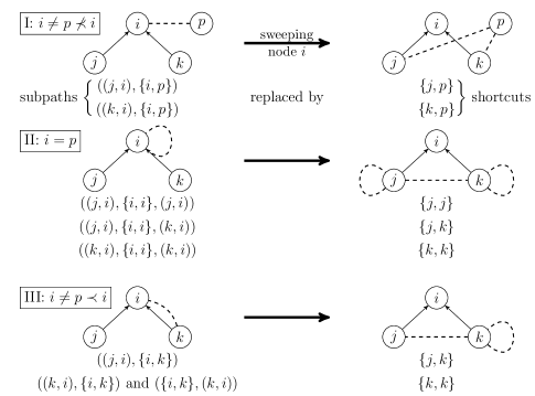
Figure 4: Pushing nonlinear arc $\{i,p\}$ is creating shortcuts.

This interpretation helps in understanding the good performance of edge_pushing in the computational tests, in the sense that only “proven” contributions to the Hessian (nonlinear arcs) are dealt with.

5.2 Example

In this section we run Algorithm 4 on one example, to better illustrate its workings. Since we’re doing it on paper, we have the luxury of doing it symbolically.

The iterations of edge_pushing on a computational graph of the function $f(x)=(x_{-2}+e^{x_{-1}})(3x_{-1}+x_{0}^{2})$ are shown on Figure 5. The thick arrows indicate the sequence of three iterations. Nodes about to be swept are highlighted. As we proceed to the graph on the right of the arrow, nonlinear arcs are created (or updated), weights are appended to edges and adjoint values are updated, except for the independent nodes, since the focus is not gradient computation. For instance, when node 3 is swept, the nonlinear arc $\{1,2\}$ is created. This nonlinear arc is pushed and split into two when node 2 is swept, becoming nonlinear arcs $\{0,1\}$ and $\{-1,1\}$, with weights $1\cdot 2v_{0}$ and $1\cdot 3$, respectively. When node 1 is swept, the nonlinear arc $\{-1,1\}$ is pushed and split into nonlinear arcs $\{-2,-1\}$ and $\{-1,-1\}$, the latter with weight $2\cdot 3\cdot e^{v_{-1}}$. Later on, in the same iteration, the nonlinear contribution of node 1, $\partial^{2}\phi_{1}/\partial v_{-1}^{2}$, is added to the nonlinear arc $\{-1,-1\}$. Other operations are analogous. The Hessian can be retrieved from the weights of the nonlinear arcs between independent nodes at the end of the algorithm:

$$f^{\prime\prime}(x)=\left(\begin{array}[]{*{3}{c}}0&3&2v_{0}\\ 3&e^{v_{-1}}(6+v_{2})&2v_{0}e^{v_{-1}}\\ 2v_{0}&2v_{0}e^{v_{-1}}&2v_{1}\end{array}\right)=\left(\begin{array}[]{*{3}{c}}0&3&2x_{0}\\ 3&e^{x_{-1}}(6+3x_{-1}+x_{0}^{2})&2x_{0}e^{x_{-1}}\\ 2x_{0}&2x_{0}e^{x_{-1}}&2(x_{-2}+e^{x_{-1}})\end{array}\right).$$

Notice that arcs that are pushed are deleted from the figure just for clarity purposes, though this is not explicitly done in Algorithm 4. Nevertheless, in the actual implementation the memory locations corresponding to these arcs are indeed deleted, or, in other words, made available, since this can be done in constant time.

 

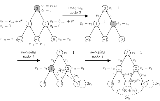
Figure 5: edge_pushing applied to a computational graph of $f(x)=(x_{-2}+e^{x_{-1}})(3x_{-1}+x_{0}^{2})$.

5.3 edge_pushing complexity bounds

For our bounds we assume that the data structure used for $W$ in Algorithm 4 is an adjacency list. This is a structure appropriate for large sparse graphs, which shall be our model for $W$, denoted by $G_{W}$. The entries in $W$ are interpreted as the set of arc weights. Thus the nodes of $G_{W}$ are associated with the rows of $W$. Notice that this is the same as the set of nodes of the computational graph. The support of $W$ is associated to the set of arcs of $G_{W}$. During the execution of the algorithm, new arcs may be created during the pushing or the creating step. After node $i$ has been swept, $G_{W}$ has accumulated all the nonlinear arcs that have been created or pushed, up to this iteration, since arcs are not deleted. On may think of $G_{W}$ as the recorded history (creation and pushing) of the nonlinear arcs.

Denote by $N_{i}$ the set of neighbors of node $i$ in $G_{W}$ and by $d_{i}$ the degree of node $i$. Of course the degree of node $i$ and its neighborhood vary during the execution of the algorithm. The time for inserting or finding an arc $\{i,j\}$ and its weight $w_{\{i,j\}}$ is bounded by $O(d_{i}+d_{j})$, where $d_{i}$ and $d_{j}$ are the degrees at the iteration where the operation takes place. We assume that the set of elemental functions is composed of only unary and binary functions.

5.3.1 Time complexity

The time complexity of edge_pushing depends on how many nonlinear arcs are allocated during execution. Thus it is important to establish bounds for the number of arcs allocated to each node. Furthermore, we may fix $G_{W}^{*}$ as the graph obtained at the end of the algorithm.

Let $d^{*}_{i}$ be the degree of node $i$ in $G_{W}^{*}$, and let $d^{*}=\max_{i}\{d_{i}^{*}\}$. Clearly $d_{i}\leq d^{*}_{i}$, where $d_{i}$ is the degree of node $i$ in the graph $G_{W}$ at any given iteration. In order to bound the complexity of edge_pushing, we consider the pushing and creating steps separately.

Studying the cases spelled out in Figure 4, one concludes that the time spent in pushing edge $\{i,p\}$ is bounded by, in each case:

Case Upper bound for time spent I: $i\neq p\nprec i$ $d_{j}^{*}+2d_{p}^{*}+d_{k}^{*}$ II: $i=p$ $d_{j}^{*}+2d_{k}^{*}$ III: $i\neq p\prec i$ $d_{j}^{*}+2d_{k}^{*}$

Hence $2(d_{j}^{*}+d_{p}^{*}+d_{k}^{*})$ is a common bound, where $j$ and $k$ are predecessors of node $i$. Since there are at most $d_{i}^{*}$ nonlinear arcs incident to node $i$, the time spent in the pushing step at the iteration where node $i$ is swept is bounded by

$$d_{i}^{*}(2(d_{j}^{*}+d_{p}^{*}+d_{k}^{*}))=O(d_{i}^{*}(d_{j}^{*}+d_{p}^{*}+d_{k}^{*}))=O(d_{i}^{*}d^{*}).$$

Finally, the assumption that all functions are either unary or binary implies that at most three nonlinear arcs are allocated during the creating step, for each iteration of edge_pushing. Hence the time used up in this step at the iteration where node $i$ is swept is bounded by

$$2(d_{j}^{*}+d_{k}^{*})=O(d_{j}^{*}+d_{k}^{*})=O(d^{*}),$$

where $j$ and $k$ are predecessors of node $i$.

Thus, taking into account the time spent in merely visiting a node — say, when the intermediate function associated with the node is linear — is constant, the time complexity of edge_pushing is

TIME(edge_pushing) $$\leq \sum_{i=1}^{\ell}(d_{i}^{*}d^{*}+d^{*}+1)$$ (33)

$$= O\left(d^{*}\sum_{i=1}^{\ell}d_{i}^{*}+\ell\right).$$

A consequence of this bound is that, if $f$ is linear, the complexity of edge_pushing is that of the function evaluation, a desirable property for Hessian algorithms.

6 Computational experiments

All tests were run on the 32-bit operating system Ubuntu 9.10, processor Intel 2.8 GHz, and 4 GB of RAM. All algorithms were coded in C and C++. The algorithm edge_pushing has been implemented as a driver of ADOL-C, and uses the taping and operator overloading functions of ADOL-C [15]. The tests aim to establish a comparison between edge_pushing and two algorithms, available as drivers of ADOL-C v. 2.1, that constitute a well established reference in the field. These algorithms incorporate the graph coloring routines of the software package ColPack [12] and the sparsity detection and Hessian-vector product procedures of ADOL-C [23]. We shall denote them by the name of the coloring scheme employed: Star and Acyclic. Analytical properties of these algorithms, as well as numerical experiments with them, have been reported in [23, 11].

We have hand-picked fifteen functions from the CUTE collection [6] and one — augmlagn — from [17] for the experiments. The selection was based on the following criteria: Hessian’s sparsity pattern, scalability and sparsity. We wanted to cover a variety of patterns; to be able to freely change the scale of the function, so as to appraise the performance of the algorithms as the dimension grows; and we wanted to work with sparse matrices. The appendix of [14] presents results for dimension values $n$ in the set $5\,000$, $20\,000$, $50\,000$ and $100\,000$, but the tables in this section always refer to the $n=50\,000$ case, unless otherwise explicitly noted.

The list of functions is presented in Table 1. The ‘Pattern’ column indicates the type of sparsity pattern: bandwidth (B $x$), arrow, box, or irregular pattern. The last two display the number of columns of the seed matrix produced by Star and Acyclic, for dimension equal to 50000. In order to report the performance of these algorithms, we briefly recall their modus operandi. Their first step, executed only once, computes a seed matrix $S$ via coloring methods, such that the Hessian $f^{\prime\prime}$ may be recovered from the product $f^{\prime\prime}S$, which involves as many Hessian-vector products as the number of columns of $S$. The latter coincides with the number of colors used in the coloring of a graph model of the Hessian. The recovery of the Hessian boils down to the solution of a linear system. Thus the first computation of the Hessian takes necessarily longer, because it comprises two steps, where the first one involves the coloring, and the second one deals with the calculation of the actual numerical entries. In subsequent Hessian computations, only the second step is executed, resulting in a shorter run. It should be noted that the number of colors is practically insensitive to changes in the dimension of the function in the examples considered, with the exception of the functions with irregular patterns, noncvxu2 and ncvxbqp1.

		# colors
Name	Pattern	Star	Acyclic
cosine	B 1	3	2
chainwoo	B 2	3	3
bc4	B 1	3	2
cragglevy	B 1	3	2
pspdoc	B 2	5	3
scon1dls	B 2	5	3
morebv	B 2	5	3
augmlagn	$5\times 5$ diagonal blocks	5	5
lminsurf	B 5	11	6
brybnd	B 5	13	7
arwhead	arrow	2	2
nondquar	arrow + B 1	4	3
sinquad	frame + diagonal	3	3
bdqrtic	arrow + B 3	8	5
noncvxu2	irregular	12	7
ncvxbqp1	irregular	12	7

Table 1: Test functions

Table 2 reports the times taken by edge_pushing and by the first and second Hessian computations by Star and Acyclic. It should be pointed out that Acyclic failed to recover the Hessian of ncvxbqp1, the last function in the table. In the examples where edge_pushing is faster than the second run of Star (resp., Acyclic), we can immediately conclude that edge_pushing is more efficient for that function, at that prescribed dimension. This was the case in 14 (resp., 16) examples. However, when the second run is faster than edge_pushing, the corresponding coloring method may eventually win, if the Hessians are computed a sufficient number of times, so as to compensate the initial time investment. This of course depends on the context in which the Hessian is used, say in a nonlinear optimization code. Thus the number of evaluations of Hessians is linked to the number of iterations of the code. The minimum time per example is highlighted in Table 2.

Table 2: Runtimes in seconds for Star, Acyclic and edge_pushing.

Focusing on the two-stage Hessian methods, we see that Star always has fastest second runtimes. Only for function sinquad is Star’s first run faster than Acyclic’s. Nevertheless, this higher investment in the first run is soon paid off, except for functions arwhead, nondquar and bdqrtic, where it would require over 1600, 50 and 25, respectively, computations of the Hessian to compensate the slower first run. We can also see from Tables 1 and 2 that Star’s performance on the second run suffers the higher the number of colors needed to color the Hessian’s graph model, which is to be expected. Thus the second runs of lminsurf, brybnd, bdqrtic, noncvxu2 and ncvxbqp1 were the slowest of Star’s. Notice that, although the Hessian of bdqrtic doesn’t require as many colors as the other four just mentioned, the function evaluation itself takes longer.

On a contrasting note, edge_pushing execution is not tied to sparsity patterns and thus this algorithm proved to be more robust, depending more on the density and number of nonlinear functions involved in the calculation. In fact, this is confirmed by looking at the variance of the runtimes for the three algorithms, see the last row of Table  2. Notice that edge_pushing has the smallest variance. Furthermore, although Star was slightly faster than edge_pushing in the second run for the functions arwhead and sinquad, the time spent in the first run was such that it would require over 4000 and 10000, respectively, evaluations of the Hessian to compensate for the slower first run.

The bar chart in Figure 6, built from the data in Table 2, permits a graphical comparison of the performances of Star and edge_pushing. Times for function brybnd deviate sharply from the remaining ones, it was a challenge for both methods. On the other hand, function ncvxbq1 presented difficulties to Star, but not to edge_pushing.

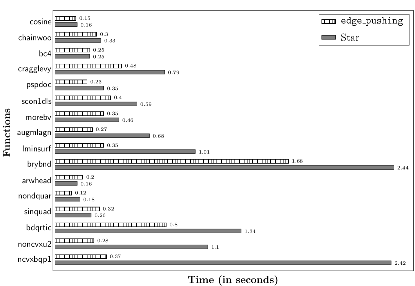
Figure 6: Graphical comparison: Star versus edge_pushing.

The bar chart containing the runtimes of the three algorithms is made pointless by the range of runtimes of Acyclic, much bigger than the other two. To circumvent this problem, we applied the base 10 log to the runtimes multiplied by 10 (just to make all logs positive). The resulting chart is depicted in Figure 7.

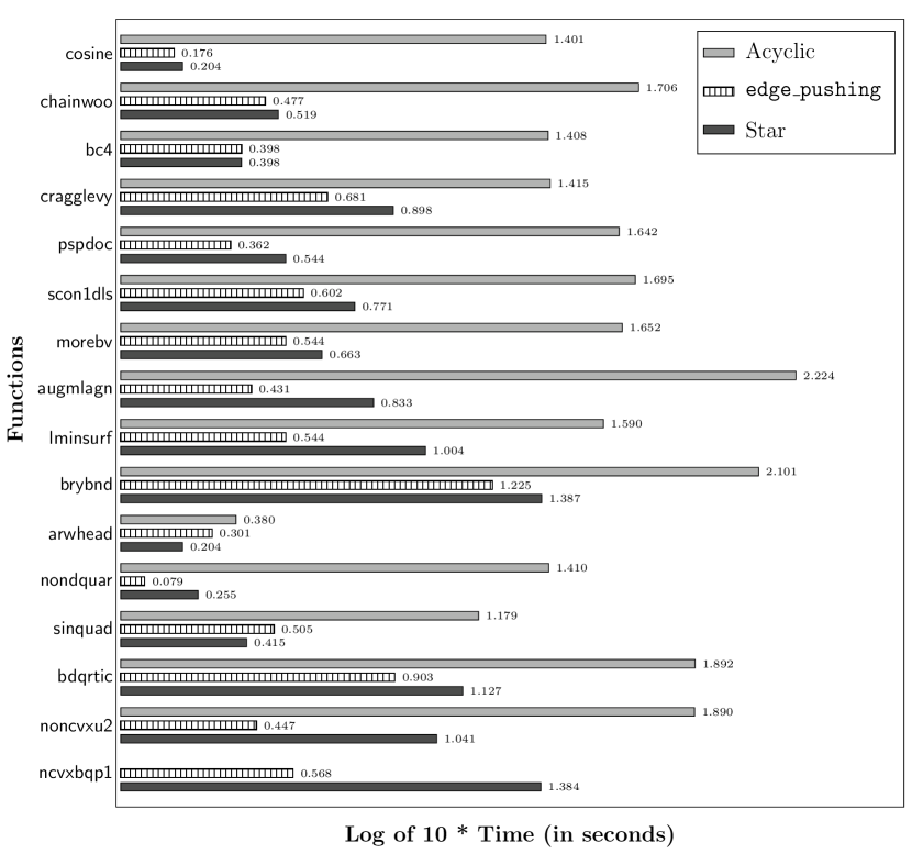
Figure 7: Graphical comparison of times in log scale: Star, Acyclic and edge_pushing.

Although the results presented in Table 2 correspond to the dimension 50000 case, they represented the general behavior of the algorithms in this set of functions. This is evidenced by the plots in Figures 8 and 9, that show the runtimes of edge_pushing and Star on four functions for dimensions varying from 5000 to 100000.

The functions cosine, sinquad, brybnd and noncvxu2 were selected for these plots because they exemplify the different phenomena we observed in the 50000 case. For instance, the performances of both edge_pushing and Star are similar in the functions cosine and sinequad, and this has happened consistently in all dimensions. Thus the dashed and solid lines in Figure 8 intertwine, and there is no striking dominance of one algorithm over the other. Also, these functions presented no real challenges, and the runtimes in all dimensions are low.

Figure 8: Evolution of runtimes of edge_pushing and Star (2nd run) with respect to dimension, for cosine and sinequad.

The function brybnd was chosen because it presented a challenge to all methods, and ncvxu2 is the representative of the functions with irregular Hessian sparsity patterns. The plots in Figure 9 show a consistent superiority of edge_pushing over Star for these two functions. All plots are close to linear, with the exception of the runtimes of Star for the function noncvxu2. We observed that the number of colors used to color the graph model of its Hessian varied quite a bit, from 6 to 21. This highest number occurred precisely for the dimension 70000, the most dissonant point in the series.

Figure 9: Evolution of runtimes of edge_pushing and Star (2nd run) with respect to dimension, for noncvxu2 and brybnd.

The appendix of [14] contains the runtimes for the three methods, including first and second runs, for all functions, for dimensions 5000, 20000 and 100000.

7 Conclusions and future research

The formula (24) for the Hessian obtained in Section 4 leads to new correctness proofs for existing Hessian computation algorithms and to the development of new ones. We also provided a graph model for the Hessian computation and both points of view inspired the construction of edge_pushing, a new algorithm for Hessian computation that conforms to Griewank and Walther’s Rule 16 of Automatic Differentiation [16, p. 240]:

The calculation of gradients by nonincremental reverse makes the corresponding computational graph symmetric, a property that should be exploited and maintained in accumulating Hessians.

The new method is a truly reverse algorithm that exploits the symmetry and sparsity of the Hessian. It is a one-phase algorithm, in the sense that there is no preparatory run where a sparsity pattern needs to be calculated that will be reused in all subsequent iterations. This can be an advantage if the function involves many intermediate functions whose second derivatives are zero in a sizable region, for instance $h(u)=(\max\{-u,0\})^{2}$. This type of function is used as a differentiable penalization of the negative axis. It is not uncommon to observe the ‘thinning out’ of Hessians over the course of nonlinear optimization, as the iterations converge to an optimum, which obviously lies in the feasible region. If the sparsity structure is fixed at the beginning, one cannot take advantaged of this slimming down of the Hessian.

edge_pushing was implemented as a driver of ADOL-C[15] and tested against two other algorithms, the Star and Acyclic methods of ColPack [12], also available as drivers of ADOL-C. Computational experiments were run on sixteen functions of the CUTE collection [6]. The results show the strong promise of the new algorithm. When compared to Star, there is a clear advantage of edge_pushing in fourteen out of the sixteen functions. In the remaining two the situation is unclear, since Star is a two-stage method and the first run can be very expensive. So even if its second run is faster than edge_pushing’s, one should take into account how many evaluations are needed in order to compensate the first run. The answers regarding the functions arwhead and sinquad were over 4000 and 10000, respectively, for dimension equal to 50000. These numbers grow with the dimension. Finally, it should be noted that edge_pushing’s performance was the more robust, and it wasn’t affected by the lack of regularity in the Hessian’s pattern.

We observed that Star was consistently better than Acyclic in all computational experiments. However, Gebremedhin et al. [11] point out that Acyclic was better than Star in randomly generated Hessians and the real-world power transmission problem reported therein, while the opposite was true for large scale banded Hessians. It is therefore mandatory to test edge_pushing not only on real-world functions, but also within the context of a real optimization problem. Only then can one get a true sense of the impact of using different algorithms for Hessian computation.

It should be pointed out that the structure of edge_pushing naturally lends itself to parallelization, a task already underway. The opposite seems to be true for Star and Acyclic. The more efficient the first run is, the less colors, or columns of the seed matrix one has, and only the task of calculating the Hessian-vector products corresponding to $f^{\prime\prime}S$ can be seen to be easily parallelizable.

Another straightforward consequence of edge_pushing is a sparsity pattern detection algorithm. This has already been implemented and tested, and will be the subject of another report.

References

- [1] R. M. Gower and M. P. Mello. A new framework for the computation of Hessians. Optimization Methods and Software, 27(2):251–273, 2012 .
- [2] Jason Abate, C. Bischof, Lucas Roh, and Alan Carle. Algorithms and design for a second-order automatic differentiation module. In Proceedings of the 1997 International Symposium on Symbolic and Algebraic Computation (Kihei, HI), pages 149–155 (electronic), New York, 1997. ACM.
- [3] F. L. Bauer. Computational graphs and rounding errors. SIAM Journal of Numerical Analysis, 11(1):87–96, 1974.
- [4] S. Bhowmick and P. D. Hovland. A polynomial-time algorithm for detecting directed axial symmetry in Hessian computational graphs. In Christian H. Bischof, H. Martin Bücker, Paul D. Hovland, Uwe Naumann, and J. Utke, editors, Advances in Automatic Differentiation, pages 91–102. Springer, 2008.
- [5] C. Bischof, G. Corliss, and A. Griewank. Structured second-and higher-order derivatives through univariate Taylor series. Optimization Methods and Software, 2(3):211–232, 1993.
- [6] I. Bongartz, A. R. Conn, Nick Gould, and Ph. L. Toint. Cute: constrained and unconstrained testing environment. ACM Trans. Math. Softw., 21(1):123–160, 1995.
- [7] R. H. Byrd, J. Nocedal, and R. A. Waltz. Knitro: An integrated package for nonlinear optimization. In Large Scale Nonlinear Optimization, 35–59, 2006, pages 35–59. Springer Verlag, 2006.
- [8] B. Christianson. Automatic Hessians by reverse accumulation. IMA J. Numer. Anal., 12(2):135–150, 1992.
- [9] L. C. W. Dixon. Use of automatic differentiation for calculating Hessians and Newton steps. In Andreas Griewank and George F. Corliss, editors, Automatic Differentiation of Algorithms: Theory, Implementation, and Application, pages 114–125. SIAM, Philadelphia, PA, 1991.
- [10] A. Forsgren, P. E. Gill, and M. H. Wright. Interior methods for nonlinear optimization. SIAM Review, 44:525–597, 2002.
- [11] A. H. Gebremedhin, A. Tarafdar, A. Pothen, and A. Walther. Efficient computation of sparse Hessians using coloring and automatic differentiation. INFORMS J. on Computing, 21(2):209–223, 2009.
- [12] A.H. Gebremedhin, D. Nguyen, M.M.A Patwary, and A. Pothen. ColPack: Graph coloring software for derivative computation and beyond. Submitted to ACM Trans. on Math. Softw., 2010.
- [13] R. M. Gower. Hessian matrices via automatic differentiation. Master’s Dissertation, Department of Applied Mathematics, Institute of Mathematics, Statistics and Scientific Computing, Unicamp, 2011. In preparation.
- [14] R. M. Gower and M. P. Mello. Hessian matrices via automatic differentiation. Technical report, Institute of Mathematics, Statistics and Scientific Computing, Unicamp, 2010.
- [15] A. Griewank, D. Juedes, H. Mitev, J. Utke, O. Vogel, and A. Walther. ADOL-C: A package for the automatic differentiation of algorithms written in C/C++. Technical report, Institute of Scientific Computing, Technical University Dresden, 1999. Updated version of the paper published in ACM Trans. Math. Software 22, 1996, 131–167.
- [16] A. Griewank and A. Walther. Evaluating derivatives. Society for Industrial and Applied Mathematics (SIAM), Philadelphia, PA, second edition, 2008. Principles and techniques of algorithmic differentiation.
- [17] W. Hock and K. Schittkowski. Test examples for nonlinear programming codes. Journal of Optimization Theory and Applications, 30(1):127–129, 1980.
- [18] W. G. Horner. A new method of solving numerical equations of all orders by continuous approximation. Philosophical Transactions of the Royal Society of London, 109:308-335, 1819.
- [19] R. H. F. Jackson and G. P. McCormick. The polyadic structure of factorable function tensors with applications to high-order minimization techniques. J. Optim. Theory Appl., 51(1):63–94, 1986.
- [20] James Stewart. Multivariable Calculus. Brooks Cole, 2007.
- [21] R. J. Vanderbei and D. F. Shanno. An interior-point algorithm for nonconvex nonlinear programming. Computational Optimization and Applications, 13:231–252, 1997.
- [22] A. Wächter and L. T. Biegler. On the implementation of an interior-point filter line-search algorithm for large-scale nonlinear programming. Math. Program., 106(1):25–57, 2006.
- [23] A. Walther. Computing sparse Hessians with automatic differentiation. ACM Trans. Math. Softw., 34(1):1–15, 2008.