Monte Carlo Simulations of BFSS
and IKKT Matrix Models

Nikhil Tanwar

A dissertation submitted for the partial fulfillment
of BS-MS dual degree in Science

[Uncaptioned image]

Indian Institute of Science Education and Research Mohali
June 2020

Certificate of Examination

This is to certify that the dissertation titled Monte Carlo Simulations of BFSS and IKKT Matrix Models submitted by Nikhil Tanwar (MS15111) for the partial fulfillment of BS-MS dual degree programme of the Institute, has been examined by the thesis committee duly appointed by the Institute. The committee finds the work done by the candidate satisfactory and recommends that the report be accepted.

Dr. Kinjalk Lochan                     Dr. Sanjib Dey                     Dr. Anosh Joseph

(Supervisor)

Dated:

Declaration

The work presented in this dissertation has been carried out by me under the guidance of Dr. Anosh Joseph at the Indian Institute of Science Education and Research Mohali.

This work has not been submitted in part or in full for a degree, a diploma, or a fellowship to any other university or institute. Whenever contributions of others are involved, every effort is made to indicate this clearly, with due acknowledgement of collaborative research and discussions. This thesis is a bonafide record of original work done by me and all sources listed within have been detailed in the bibliography.

Nikhil Tanwar

(Candidate)

Dated:

In my capacity as the supervisor of the candidate’s project work, I certify that the above statements by the candidate are true to the best of my knowledge.

Dr. Anosh Joseph

(Supervisor)

Acknowledgment

I express my sincere gratitude to my supervisor, Dr. Anosh Joseph for his patience, motivation, prudent comments, valuable suggestions, and beneficial information, which have helped me remarkably in my research and in writing this thesis. His enormous knowledge and thorough experience in lattice field theory have enabled me to complete this research successfully. I am incredibly thankful to him for sparing his precious time to guide me, clarifying my queries, correcting me during my research and sharing his workstation without which simulations would have never been completed.

Besides my advisor, I wish to thank the rest of my thesis committee members, Dr. Kinjalk Lochan and Dr. Sanjib Dey, for their insightful comments and encouragement.

I extend my sincere thanks to Mr. Arpith Kumar for giving his valuable time for the discussion sessions and for helping me during the simulation of the BFSS Matrix model. I also extend my sincere thanks to Mr. Adeeb Mev for the collaboration we made for the simulation of the BFSS matrix model.

I acknowledge IISER Mohali for providing me with the best infrastructure and environment for carrying out this project. I am also thankful to the Department of Science and Technology (DST), Government of India, for supporting me with the institute fellowship during the past five years.

I want to thank my batchmates and friends for interesting peer discussions throughout the five years of the course. I am thankful to Nilangshu Bhattacharyya, Amit Suthar, Adarsh Bhardwaj, Anubhav Jindal, Apoorv Gaurav, Debanjan Chowdhury, Debjit Ghosh, Gaurav Singh, Ishan Sarkar, Paresh Nath Das, Satyam Prakash, Swastik P G, Vidur Sury and Vivek Jadhav. I would also like to thank all my friends listed above for their continuous moral support and motivation throughout this journey without which it would have been a very tough journey.

I would also like to thank and acknowledge my parents and my brother Dhruv Tanwar for their love and support throughout the years of my study. This would not have been possible without them.

Abstract

In this thesis, we studied the bosonic BFSS and IKKT matrix models using Monte Carlo simulations. First, we explored some toy models to check the validity of the numerical simulations. Then we simulated the BFSS matrix model using Hamiltonian Monte Carlo (HMC) algorithm. In the BFSS matrix model, we used the Polyakov loop as an order parameter to investigate the large-N𝑁N behaviour of this model at different temperatures. Our simulations confirmed that the model exhibits a confinement-deconfinement phase transition as the temperature of the system is varied. Besides the Polyakov loop, other observables such as internal energy and extent of space were also computed. In the bosonic IKKT model, we studied the spontaneous symmetry breaking (SSB) of SO(10)𝑆𝑂10SO(10) symmetry using the moment of inertia tensor and found that there is no SSB of SO(10)𝑆𝑂10SO(10) symmetry in this model. Besides the eigenvalues of the moment of inertia tensor, other observable such as extent of spacetime was also computed. We also studied the simulation theory of the phase-quenched IKKT model.

Chapter 1 Introduction

String theory is believed to be a very promising candidate for the theory of everything. It attempts to unify the theory of gravity with other three fundamental forces of nature: Electromagnetism, Strong and Weak nuclear forces. It replaces the point like particles, which is the fundamental assumption of the Standard Model of particle physics, by one-dimensional objects called strings. All the matter particles as well as the force carrying particles are made up of these strings and the theory explains how these strings propagate in spacetime and interact with each other. In string theory, each of the fundamental particle is represented by the unique vibrational frequency of the string.

Till today there are five consistent superstring theories: type I, type IIA, type IIB, heterotic SO(32)𝑆𝑂32SO(32) and heterotic E8×E8subscript𝐸8subscript𝐸8E_{8}\times E_{8}. These theories differ whether the strings are open or closed, whether the strings are oriented or not and on how they treat electrical charges. All of these theories are in 10-dimensional spacetime and all the calculations are done perturbatively in terms of string length lssubscript𝑙𝑠l_{s} and string coupling gssubscript𝑔𝑠g_{s}.

It has been found that all of these different string theories are connected to each other through some transformation (T-duality, S-duality etc.) and this led to the conjecture in 1995 by Edward Witten [Witten 95] that they are part of some bigger theory called M-theory. M-theory is still undiscovered but it is known that it lives in 11 dimensions and it is a non-perturbative theory. The M in M-theory is undefined and sometimes it is referred to as “membrane” or “matrix.”

String theory was first studied in the late 1960s as a model of strong interaction and from 1974 onwards proper study of string theory started and since then it has been evolving. Even today, there is a debate over its validity as no part of this theory has been experimentally verified.

1.1 BFSS Matrix Model

BFSS Model was conjectured in 1996 by T. Banks, W. Fischler, S. H. Shenker, and L. Susskind [Banks 97]. This model is one dimensional supersymmetric Yang-Mills theory and this theory acts as the low energy effective description of D0𝐷0D0-branes of type IIA superstring theory [Filev 16] and in the limit N𝑁N\to\infty it is believed that this theory will represent M-theory. One of the methods to obtain the action of this theory is by dimensionally reducing the 𝒩=1𝒩1\mathcal{N}=1 super Yang-Mills theory in 9+1 dimensions with gauge group SU(N)𝑆𝑈𝑁SU(N) to 0+1 dimensions (See Appendix A). The resulting action is given by

S=12g2𝑑tTr((DtXi)2+12[Xi,Xj]2iΨαTC10γαβ0DtΨβ+ΨαTC10γαβi[Xi,Ψβ]missing).𝑆12superscript𝑔2differential-d𝑡tracesuperscriptsubscript𝐷𝑡subscript𝑋𝑖212superscriptsubscript𝑋𝑖subscript𝑋𝑗2𝑖subscriptsuperscriptΨ𝑇𝛼subscript𝐶10subscriptsuperscript𝛾0𝛼𝛽subscript𝐷𝑡subscriptΨ𝛽subscriptsuperscriptΨ𝑇𝛼subscript𝐶10subscriptsuperscript𝛾𝑖𝛼𝛽subscript𝑋𝑖subscriptΨ𝛽missingS=\frac{1}{2g^{2}}\int dt\,\Tr\Bigg((D_{t}X_{i})^{2}+\frac{1}{2}[X_{i},X_{j}]^{2}-i\Psi^{T}_{\alpha}C_{10}\gamma^{0}_{\alpha\beta}D_{t}\Psi_{\beta}+\Psi^{T}_{\alpha}C_{10}\gamma^{i}_{\alpha\beta}[X_{i},\Psi_{\beta}]\Bigg{missing}). (1.1)

where Dt=ti[A(t),]subscript𝐷𝑡subscript𝑡𝑖𝐴𝑡D_{t}=\partial_{t}-i[A(t),\cdot]; i,j=1,2,,9formulae-sequence𝑖𝑗129i,j=1,2,\cdots,9; α,β=1, 2,, 32formulae-sequence𝛼𝛽1232\alpha,\,\beta=1,\,2,\,\cdots,\,32; Xisuperscript𝑋𝑖X^{i} are N×N𝑁𝑁N\times N traceless Hermitian matrices; g𝑔g is the one-dimensional Yang-Mills coupling; A(t)𝐴𝑡A(t) is the one-dimensional gauge field; ΨΨ\Psi is a 32-component Majorana-Weyl fermion with each component of the fermion being an N×N𝑁𝑁N\times N traceless Hermitian matrix; C10subscript𝐶10C_{10} is the charge conjugation matrix in the ten dimensions; and γisuperscript𝛾𝑖\gamma^{i} are the gamma matrices in ten dimensions. The action is invariant under the following set of gauge transformations

Xi(t)superscript𝑋𝑖𝑡\displaystyle X^{i}(t) \displaystyle\longrightarrow V(t)Xi(t)V(t),𝑉𝑡superscript𝑋𝑖𝑡superscript𝑉𝑡\displaystyle V(t)X^{i}(t)V^{\dagger}(t), (1.2)
A(t)𝐴𝑡\displaystyle A(t) \displaystyle\longrightarrow V(t)(A(t)+it)V(t),𝑉𝑡𝐴𝑡𝑖subscript𝑡superscript𝑉𝑡\displaystyle V(t)\left(A(t)+i\partial_{t}\right)V^{\dagger}(t), (1.3)
Ψα(t)subscriptΨ𝛼𝑡\displaystyle\Psi_{\alpha}(t) \displaystyle\longrightarrow V(t)Ψα(t)V(t),𝑉𝑡subscriptΨ𝛼𝑡superscript𝑉𝑡\displaystyle V(t)\,\Psi_{\alpha}(t)\,V^{\dagger}(t), (1.4)

where V(t)SU(N)𝑉𝑡𝑆𝑈𝑁V(t)\in SU(N).

1.2 BFSS Model and Black Hole thermodynamics

One of the motivations to study the BFSS model is the connection of this model with the black hole states. The finite temperature states of BFSS model is related to the black hole states of type IIA supergravity [Klebanov 98] [Banks 98]. The connection between BFSS matrix model and the black hole states has also been discussed in the Ref. [Kabat 01a] [Kabat 01b]. In these two references, the authors calculated the entropy of a black hole in strongly coupled quantum mechanics beginning with the Bekenstein-Hawking entropy of a ten-dimensional non-extremal back hole. The free energy of the black hole in terms of the parameters of the gauge theory (here the BFSS model) can be written as

FT=4.115N2(T3gym2N)3/5.𝐹𝑇4.115superscript𝑁2superscriptsuperscript𝑇3subscriptsuperscript𝑔2𝑦𝑚𝑁35\displaystyle\frac{F}{T}=-4.115N^{2}\left(\frac{T^{3}}{g^{2}_{ym}N}\right)^{3/5}. (1.5)

The above formula is of interest for a couple of reasons. First, its dependence on the ’t Hooft coupling. The limit N𝑁N\to\infty corresponds to the region where supergravity is valid and therefore it is the appropriate limit to look for black holes in the BFSS model. Second reason being that the free energy depends on N2superscript𝑁2N^{2}, which is the expected behaviour of a gauge theory in the deconfined phase.

It would be important to reproduce this formula from the matrix model. To get this behaviour in the matrix model, one must look in the strong coupling, which is not accessible in the perturbation theory. That is, in a regime where it is highly impossible to carry out an analytical calculation to derive this expression. Thus we are left with numerical simulations as these technique does not have any such restrictions.

1.3 Phase Transition

For a system with a density of states that grows exponentially,

ρ(E)eβHEsimilar-to𝜌𝐸superscript𝑒subscript𝛽𝐻𝐸\displaystyle\rho(E)\sim e^{\beta_{H}E} (1.6)

there exist an upper limit to the temperature known as the Hagedorn temperature. Above this temperature the partition function diverges [Furuuchi 03]

limTTHTr(eβH).subscript𝑇superscriptsubscript𝑇𝐻tracesuperscript𝑒𝛽𝐻\displaystyle\lim\limits_{T\to T_{H}^{-}}\Tr(e^{-\beta H})\to\infty. (1.7)

Above this cutoff temperature THsubscript𝑇𝐻T_{H}, partition function does not exist. However, it can be made to exist if we keep N𝑁N large but finite. Performing this breaks the exponential growth in the asymptotic density of states at some large but finite energy value. For temperature greater than THsubscript𝑇𝐻T_{H}, the entropy and the energy are dominated by the states at and above the cutoff scale and the free energy jumps from 𝒪(1)𝒪1\mathcal{O}(1) to 𝒪(N2)𝒪superscript𝑁2\mathcal{O}(N^{2}) [Hadizadeh 05]. Thus

limNFN2subscript𝑁𝐹superscript𝑁2\displaystyle\lim\limits_{N\to\infty}\frac{F}{N^{2}} =\displaystyle= 0(Confined phase),0(Confined phase)\displaystyle 0\qquad\textrm{(Confined phase)}, (1.8)
limNFN2subscript𝑁𝐹superscript𝑁2\displaystyle\lim\limits_{N\to\infty}\frac{F}{N^{2}} \displaystyle\neq 0(Deconfined phase).0(Deconfined phase)\displaystyle 0\qquad\textrm{(Deconfined phase)}. (1.9)

The transition from the confined phase to deconfined phase is known as confinement-deconfinement phase transition or deconfinement phase transition. In the confined phase, the quantum states of the Hamiltonian should be singlets under the gauge symmetry [SEMENOFF 04]. This condition fails as soon as the system reaches the Hagedorn temperature. This type of transition is found in large-N𝑁N gauge theories, such as weakly coupled Yang-Mills theory and it is also expected to be found in the BFSS model [SEMENOFF 04].

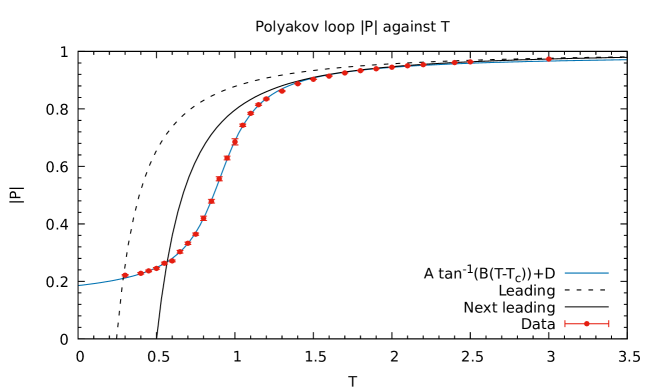
This confinement-deconfinement phase transition in the matrix models is associated with the breakdown of the center symmetry, i.e., A(t)A(t)+k𝟙𝐴𝑡𝐴𝑡𝑘1A(t)\to A(t)+k\mathbb{1}. The order parameter for this symmetry breaking is the Polyakov loop [Polyakov 78]. Polyakov loop is defined as the trace of the holonomy of the gauge field around the finite temperature Euclidean time circle

P=1NTr(P(ei𝑑tA(t))).𝑃1𝑁trace𝑃superscript𝑒𝑖contour-integraldifferential-d𝑡𝐴𝑡\displaystyle P=\frac{1}{N}\Tr(P(e^{i\oint dt\,A(t)})). (1.10)

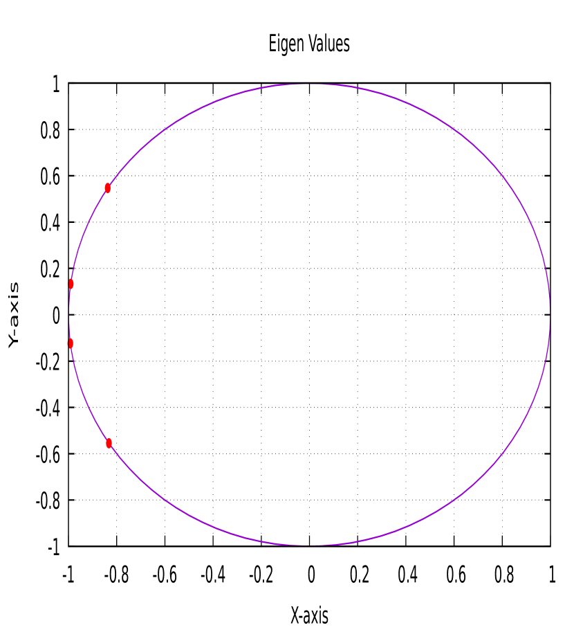
This operator is gauge invariant as it is a special case of the Wilson line operator. The expectation value of this operator is zero in confined phase and it jumps to a non-zero value as we cross the phase transition point and enters the deconfined phase. This is simply because Polyakov loop is a unitary matrix and its eigenvalues are uniformly distributed on the unit circle in the confined phase and in the deconfined phase the eigenvalues clump towards a single point. We have

Pdelimited-⟨⟩𝑃\displaystyle\left\langle P\right\rangle =\displaystyle= 0(Confined phase),0(Confined phase)\displaystyle 0\qquad\textrm{(Confined phase)}, (1.11)
Pdelimited-⟨⟩𝑃\displaystyle\left\langle P\right\rangle \displaystyle\neq 0(Deconfined phase).0(Deconfined phase)\displaystyle 0\qquad\textrm{(Deconfined phase)}. (1.12)

We use this as an order parameter for our simulations of the BFSS model.

1.4 IKKT Matrix Model

IKKT model was conjectured in 1997 by N. Ishibashi, H. Kawai, Y. Kitazawa, A. Tsuchiya [Ishibashi 97]. This model was proposed as a non-perturbative formulation of superstring theory. This model is also known as type IIB matrix model. The action of this model can be obtained by dimensionally reducing the 𝒩=1𝒩1\mathcal{N}=1 super Yang-Mills theory in 9+1 dimensions with gauge group SU(N)𝑆𝑈𝑁SU(N) to 0+0000+0 dimensions (See Appendix A). The resulting Euclidean action is given by

SE=14g2Tr([Xi,Xj]2)12g2Tr(ΨαTC10γαβi[Xi,Ψβ]),subscript𝑆E14superscript𝑔2tracesuperscriptsubscript𝑋𝑖subscript𝑋𝑗212superscript𝑔2tracesubscriptsuperscriptΨ𝑇𝛼subscript𝐶10subscriptsuperscript𝛾𝑖𝛼𝛽subscript𝑋𝑖subscriptΨ𝛽\displaystyle S_{\rm E}=-\frac{1}{4g^{2}}\Tr([X_{i},X_{j}]^{2})-\frac{1}{2g^{2}}\Tr(\Psi^{T}_{\alpha}C_{10}\gamma^{i}_{\alpha\beta}[X_{i},\Psi_{\beta}]), (1.13)

where i,j=1,2,,10formulae-sequence𝑖𝑗1210i,j=1,2,\cdots,10; α,β=1, 2,, 32formulae-sequence𝛼𝛽1232\alpha,\,\beta=1,\,2,\,\cdots,\,32; Xisuperscript𝑋𝑖X^{i} are N×N𝑁𝑁N\times N traceless Hermitian matrices; g𝑔g is the zero-dimensional Yang-Mills coupling; ΨΨ\Psi is a 32-component Majorana-Weyl fermion with each component of the fermion being an N×N𝑁𝑁N\times N traceless Hermitian matrix; C10subscript𝐶10C_{10} is the Euclidean charge conjugation matrix in ten dimensions; and γisuperscript𝛾𝑖\gamma^{i} are the Euclidean gamma matrices in ten dimensions. The action is invariant under the following set of gauge transformations

Xisubscript𝑋𝑖\displaystyle X_{i} \displaystyle\longrightarrow VXiV,𝑉subscript𝑋𝑖superscript𝑉\displaystyle V\,X_{i}\,V^{\dagger}, (1.14)
ΨαsubscriptΨ𝛼\displaystyle\Psi_{\alpha} \displaystyle\longrightarrow VΨα(x)V.𝑉subscriptΨ𝛼𝑥superscript𝑉\displaystyle V\,\Psi_{\alpha}(x)\,V^{\dagger}. (1.15)

1.5 Motivation for IKKT Model

One of the main motivations to study the IKKT model is that in the large-N𝑁N limit, spacetime emerges dynamically in this model from the eigenvalues of the ten bosonic matrices and this tells us that dynamical compactification can be viewed as a purely non-perturbative effect [Aoki 98]. The evidence for the same came from the simulations of the Lorentzian version of the IKKT model [Nishimura 19, Nishimura 20]. In these simulations it has been found that continuous time emerges dynamically and three-dimensional space undergoes expansion after a critical time with the other six spatial dimensions remaining small. The expansion is exponential at early times [Ito 14], which becomes a power law at later times [Ito 15]. These two results provide evidence that a realistic cosmological scenario may also arise dynamically from this model.

On the other hand, we can also look for dynamical compactification of extra dimensions in the Euclidean model by spontaneous symmetry breaking (SSB) of the SO(10)𝑆𝑂10SO(10) due to the fluctuations of the phase of the Pffafian for SO(d)𝑆𝑂𝑑SO(d) symmetric configurations with larger d𝑑d [Nishimura 00]. It has been showed that SSB does not take place in phase-quenched model, so SSB is attributed to the effect of the phase of the Pffafian [Ambjørn 00]. It was also shown that in the IKKT model that the SO(3)𝑆𝑂3SO(3) symmetric vacuum has the lowest free energy, which implies SSB to SO(3)𝑆𝑂3SO(3) [Nishimura 11]. Recent work on this model using complex Langevin algorithm showed that there is SSB of SO(10)𝑆𝑂10SO(10) to SO(3)×SO(7)𝑆𝑂3𝑆𝑂7SO(3)\times SO(7) [Anagnostopoulos 20]. They further showed that the SO(7)𝑆𝑂7SO(7) symmetry is also broken into smaller groups.

1.6 Path Integral and Statistical Mechanics

In this section will introduce how the path integrals in quantum field theory and statistical mechanics are connected. We will explain this using the example of a real scalar field.

Let us consider a theory containing a scalar field defined by the following action

S[ϕ(x)]=0t𝑑td3x(12μϕμϕV(ϕ)),𝑆delimited-[]italic-ϕ𝑥superscriptsubscript0𝑡differential-d𝑡superscriptsuperscript𝑑3𝑥12subscript𝜇italic-ϕsuperscript𝜇italic-ϕ𝑉italic-ϕ\displaystyle S[\phi(x)]=\int\limits_{0}^{t}dt{{}^{\prime}}\int d^{3}x\left(\frac{1}{2}\partial_{\mu}\phi\partial^{\mu}\phi-V(\phi)\right), (1.16)

where V(ϕ)𝑉italic-ϕV(\phi) is the potential functional. Then the probability amplitude to go from the field configurations ϕ1(x)subscriptitalic-ϕ1𝑥\phi_{1}(\vec{x}) to ϕ2(x)subscriptitalic-ϕ2𝑥\phi_{2}(\vec{x}) in time t𝑡t is given by the path integral G(ϕ2(x),ϕ1(x);t)𝐺subscriptitalic-ϕ2𝑥subscriptitalic-ϕ1𝑥𝑡G(\phi_{2}(\vec{x}),\phi_{1}(\vec{x});t). We have

G(ϕ2(x),ϕ1(x);t)𝐺subscriptitalic-ϕ2𝑥subscriptitalic-ϕ1𝑥𝑡\displaystyle G(\phi_{2}(\vec{x}),\phi_{1}(\vec{x});t) =\displaystyle= ϕ2(x)|eiHt|ϕ1(x),quantum-operator-productsubscriptitalic-ϕ2𝑥superscript𝑒𝑖𝐻𝑡subscriptitalic-ϕ1𝑥\displaystyle\langle\phi_{2}(\vec{x})|e^{-iHt}|\phi_{1}(\vec{x})\rangle, (1.17)
G(ϕ2(x),ϕ1(x);t)𝐺subscriptitalic-ϕ2𝑥subscriptitalic-ϕ1𝑥𝑡\displaystyle G(\phi_{2}(\vec{x}),\phi_{1}(\vec{x});t) =\displaystyle= ϕ(x,0)=ϕ1(x)ϕ(x,t)=ϕ2(x)𝒟ϕeiS[ϕ(x)],superscriptsubscriptitalic-ϕ𝑥0subscriptitalic-ϕ1𝑥italic-ϕ𝑥𝑡subscriptitalic-ϕ2𝑥𝒟italic-ϕsuperscript𝑒𝑖𝑆delimited-[]italic-ϕ𝑥\displaystyle\int\limits_{\phi(\vec{x},0)=\phi_{1}(\vec{x})}^{\phi(\vec{x},t)=\phi_{2}(\vec{x})}\,\mathcal{D}\phi\,\,e^{iS[\phi(x)]}, (1.18)

where H𝐻H is the Hamiltonian of this system. The partition function for the theory of scalar field is given by

Z=Tr(eβH)=𝒟ϕ(x)ϕ(x)|eβH|ϕ(x).𝑍tracesuperscript𝑒𝛽𝐻𝒟italic-ϕ𝑥quantum-operator-productitalic-ϕ𝑥superscript𝑒𝛽𝐻italic-ϕ𝑥\displaystyle Z=\Tr(e^{-\beta H})=\int\mathcal{D}\phi(\vec{x})\,\,\langle\phi(\vec{x})|e^{-\beta H}|\phi(\vec{x})\rangle. (1.19)

If we perform a Wick rotation (see Appendix A), i.e., t=itE𝑡𝑖subscript𝑡𝐸t=-it_{E}, then we go to the Euclidean signature from the Minkowski signature and we can use that to write

ϕ(x)|eβH|ϕ(x)=ϕ(x,0)=ϕ(x)ϕ(x,β)=ϕ(x)𝒟ϕeSE[ϕ(x)]=G(ϕ(x),ϕ(x);iβ),quantum-operator-productitalic-ϕ𝑥superscript𝑒𝛽𝐻italic-ϕ𝑥superscriptsubscriptitalic-ϕ𝑥0italic-ϕ𝑥italic-ϕ𝑥𝛽italic-ϕ𝑥𝒟italic-ϕsuperscript𝑒subscript𝑆𝐸delimited-[]italic-ϕ𝑥𝐺italic-ϕ𝑥italic-ϕ𝑥𝑖𝛽\displaystyle\langle\phi(\vec{x})|e^{-\beta H}|\phi(\vec{x})\rangle=\int\limits_{\phi(\vec{x},0)=\phi(\vec{x})}^{\phi(\vec{x},\beta)=\phi(\vec{x})}\,\mathcal{D}\phi\,\,e^{-S_{E}[\phi(x)]}=G(\phi(\vec{x}),\phi(\vec{x});-i\beta), (1.20)

where

SE[ϕ(x)]=0β𝑑tEd3x(12μϕμϕ+V(ϕ))subscript𝑆𝐸delimited-[]italic-ϕ𝑥superscriptsubscript0𝛽differential-dsubscript𝑡𝐸superscript𝑑3𝑥12subscript𝜇italic-ϕsubscript𝜇italic-ϕ𝑉italic-ϕS_{E}[\phi(x)]=\displaystyle\int\limits_{0}^{\beta}dt_{E}\int d^{3}x\left(\frac{1}{2}\partial_{\mu}\phi\partial_{\mu}\phi+V(\phi)\right) (1.21)

is the Euclidean action. If we substitute this in Eq. (1.19), the partition function becomes

Z𝑍\displaystyle Z =\displaystyle= 𝒟ϕ(x)ϕ(x)|eβH|ϕ(x)𝒟italic-ϕ𝑥quantum-operator-productitalic-ϕ𝑥superscript𝑒𝛽𝐻italic-ϕ𝑥\displaystyle\int\mathcal{D}\phi(\vec{x})\,\,\langle\phi(\vec{x})|e^{-\beta H}|\phi(\vec{x})\rangle (1.22)
=\displaystyle= 𝒟ϕ(x)ϕ(x,0)=ϕ(x)ϕ(x,β)=ϕ(x)𝒟ϕeSE[ϕ(x)]𝒟italic-ϕ𝑥superscriptsubscriptitalic-ϕ𝑥0italic-ϕ𝑥italic-ϕ𝑥𝛽italic-ϕ𝑥𝒟italic-ϕsuperscript𝑒subscript𝑆𝐸delimited-[]italic-ϕ𝑥\displaystyle\int\mathcal{D}\phi(\vec{x})\int\limits_{\phi(\vec{x},0)=\phi(\vec{x})}^{\phi(\vec{x},\beta)=\phi(\vec{x})}\,\mathcal{D}\phi\,\,e^{-S_{E}[\phi(x)]}
=\displaystyle= PBC𝒟ϕeSE[ϕ],subscriptcontour-integral𝑃𝐵𝐶𝒟italic-ϕsuperscript𝑒subscript𝑆𝐸delimited-[]italic-ϕ\displaystyle\oint\limits_{PBC}\mathcal{D}\phi\,\,e^{-S_{E}[\phi]},

where PBC stands for periodic boundary conditions, i.e., ϕ(x,0)=ϕ(x,β)italic-ϕ𝑥0italic-ϕ𝑥𝛽\phi(\vec{x},0)=\phi(\vec{x},\beta). If we perform the same calculation for fermionic fields we will get the same result but in place of periodic boundary conditions we will have anti-periodic boundary conditions, i.e., ψ(x,0)=ψ(x,β)𝜓𝑥0𝜓𝑥𝛽\psi(\vec{x},0)=-\psi(\vec{x},\beta). Using this formalism we can study the physics of finite temperature quantum field theory. This formalism is also useful in exploring strongly coupled quantum field theories using Monte Carlo simulations of the Euclidean model.

So a general result for fields in flat Minkowski spacetime follows from here: Euclidean quantum field theory in (D+1)𝐷1(D+1)-dimensional spacetime with 0tE<β0subscript𝑡𝐸𝛽0\leq t_{E}<\beta is the same as the quantum statistical mechanics in D𝐷D-dimensional space [Zee 10].

Chapter 2 Markov Chain Monte Carlo Algorithms

This chapter introduces the computational techniques required to sample data from a probability distribution (PD) that is known up to some multiplicative constants. We will see how to apply these algorithms to the Euclidean path integrals in this and later chapters. To begin, consider a general partition function of a particle in one dimension in some potential V(x)𝑉𝑥V(x), given by

Z=𝒟x(t)eSE[x(t)],𝑍𝒟𝑥𝑡superscript𝑒subscript𝑆𝐸delimited-[]𝑥𝑡\displaystyle Z=\int\mathcal{D}x(t)\,\,e^{-S_{E}[x(t)]}, (2.1)

where the Euclidean action for a general potential V(x)𝑉𝑥V(x) is given by

SE[x(t)]=0β𝑑t(12x˙2+V(x)),subscript𝑆𝐸delimited-[]𝑥𝑡superscriptsubscript0𝛽differential-d𝑡12superscript˙𝑥2𝑉𝑥\displaystyle S_{E}[x(t)]=\int\limits_{0}^{\beta}dt\left(\dfrac{1}{2}\dot{x}^{2}+V(x)\right), (2.2)

with periodic boundary conditions x(t+β)=x(t)𝑥𝑡𝛽𝑥𝑡x(t+\beta)=x(t) (for bosonic fields). Since we are using the canonical ensemble, the system is at temperature given by T=β1𝑇superscript𝛽1T=\beta^{-1}. Now if we were able to calculate Z𝑍Z, then we can calculate thermodynamic quantities like free energy, energy, and other quantities using Z𝑍Z and derivatives of it.

But for a general potential V(x)𝑉𝑥V(x) it cannot be solved exactly. So we need to resort to other methods to calculate the expectation values. One method is to use perturbative calculations using Feynman diagrams. But this method breaks down for strong-coupling terms present in the potential function as the contribution of the higher order diagrams are comparable to the previous diagrams. So we need to resort to non-perturbative methods for those cases.

One of the methods to evaluate these expectation values is through numerical simulations. But our system is continuous, and so the partition function is to be integrated over dynamical variables at all times. The standard way to do this is to divide the time variable into slices and evaluate each spatial integral at a fixed time [Peskin 95]. First we discretize the time variable by dividing the time variable into a lattice of T𝑇T points with uniform lattice spacing a𝑎a with β=aT𝛽𝑎𝑇\beta=aT. Now the dynamical variable x(t)𝑥𝑡x(t) is no longer continuous and exists only on the discrete lattice points xtsubscript𝑥𝑡x_{t}. So our partition function on the lattice becomes

Z=(t=1Tdxt)eSlat(xt),𝑍superscriptsubscriptproduct𝑡1𝑇𝑑subscript𝑥𝑡superscript𝑒subscript𝑆latsubscript𝑥𝑡\displaystyle Z=\int\left(\prod\limits_{t=1}^{T}dx_{t}\right)e^{-S_{\rm lat}(x_{t})}, (2.3)

where Slatsubscript𝑆latS_{\rm lat} is the lattice action. We can construct this action by discretizing SEsubscript𝑆𝐸S_{E}. For this, we need to replace integrals with finite sums and derivatives with finite differences. The prescription to do this is as follows

x(t)𝑥𝑡\displaystyle x(t)\,\, xt,absentsubscript𝑥𝑡\displaystyle\longrightarrow\,\,x_{t}, (2.4)
xt𝑥𝑡\displaystyle\frac{\partial x}{\partial t}\,\, xtxt1a,absentsubscript𝑥𝑡subscript𝑥𝑡1𝑎\displaystyle\longrightarrow\,\,\frac{x_{t}-x_{t-1}}{a}, (2.5)
0βsuperscriptsubscript0𝛽\displaystyle\int\limits_{0}^{\beta}\,\, at=1T,absent𝑎superscriptsubscript𝑡1𝑇\displaystyle\longrightarrow\,\,a\sum\limits_{t=1}^{T}, (2.6)
V(x(t))𝑉𝑥𝑡\displaystyle V(x(t))\,\, V(xt).absent𝑉subscript𝑥𝑡\displaystyle\longrightarrow\,\,V(x_{t}). (2.7)

This prescription works well only for bosonic fields. The description to put gauge fields and fermionic fields on the lattice will be discussed in the later chapters. Since bosonic fields follow periodic boundary conditions we also need to maintain that condition on the lattice. On the lattice, periodic boundary condition becomes xt=xt+Tsubscript𝑥𝑡subscript𝑥𝑡𝑇x_{t}=x_{t+T}. So with this prescription lattice action Slatsubscript𝑆latS_{\rm lat} is given by

Slat=at=1T[12(xtxt1a)2+V(xt)],subscript𝑆lat𝑎superscriptsubscript𝑡1𝑇delimited-[]12superscriptsubscript𝑥𝑡subscript𝑥𝑡1𝑎2𝑉subscript𝑥𝑡\displaystyle S_{\rm lat}=a\sum\limits_{t=1}^{T}\left[\frac{1}{2}\left(\frac{x_{t}-x_{t-1}}{a}\right)^{2}+V(x_{t})\right], (2.8)

with x0=xTsubscript𝑥0subscript𝑥𝑇x_{0}=x_{T}. The above method describes the behaviour of the partition function up to some multiplicative constant provided that enough number of lattice sites are used so that system behaves as if it is a continuous system.

Now we can use the above form of the partition function to calculate the expectation values of observables. For some observable 𝒪𝒪\mathcal{O}, the expectation value 𝒪delimited-⟨⟩𝒪\left\langle\mathcal{O}\right\rangle is given by

𝒪=(t=1Tdxt)𝒪(xt)eSlat(xt)(t=1Tdxt)eSlat(xt).delimited-⟨⟩𝒪superscriptsubscriptproduct𝑡1𝑇𝑑subscript𝑥𝑡𝒪subscript𝑥𝑡superscript𝑒subscript𝑆latsubscript𝑥𝑡superscriptsubscriptproduct𝑡1𝑇𝑑subscript𝑥𝑡superscript𝑒subscript𝑆latsubscript𝑥𝑡\displaystyle\left\langle\mathcal{O}\right\rangle=\dfrac{\displaystyle\int\left(\prod\limits_{t=1}^{T}dx_{t}\right)\,\mathcal{O}(x_{t})\,e^{-S_{\rm lat}(x_{t})}}{\displaystyle\int\left(\prod\limits_{t=1}^{T}dx_{t}\right)e^{-S_{\rm lat}(x_{t})}}. (2.9)

Now we can evaluate this expression numerically. But if we use simple numerical integration techniques (e.g., Gauss’ quadrature, Simpson’s rule), evaluating the above integral becomes a computationally heavy task. We can understand this using a simple argument. For one-dimensional integral, we need to divide the integration region into grids, let us say, N𝑁N grids. If we now consider a d𝑑d-dimensional integral then we would require Ndsuperscript𝑁𝑑N^{d} grids to evaluate the integral numerically. For better accuracy we need N𝑁N to be large, so the complexity of the algorithm is 𝒪(Nd)𝒪superscript𝑁𝑑\mathcal{O}(N^{d}). For example, if we take 20 lattice points and the number of grids to be 100, then we need to sum 10020=1040superscript10020superscript1040100^{20}=10^{40} terms, which is a huge number. Apart from this, there will be regions in the integration domain where the contribution to integral will be negligible as the weight factor here is eSlat(xt)superscript𝑒subscript𝑆latsubscript𝑥𝑡e^{-S_{\rm lat}(x_{t})}. This way, we are going to waste computational resources on these integration regions. So we require more clever methods to evaluate the above integral. Such methods may give more importance to the volume of the integration region that contributes the most to the integral.

2.1 Importance Sampling

In any Monte Carlo integration, the error is proportional to the standard deviation of the integrand and inversely proportional to the sample size. One way to reduce the error is to reduce the standard deviation as it does not cost more computational power. This is done by sampling the important region of the integral.

Let us say we have an integral

I=abf(x)𝑑x,𝐼superscriptsubscript𝑎𝑏𝑓𝑥differential-d𝑥\displaystyle I=\int\limits_{a}^{b}f(x)dx, (2.10)

and we have a probability distribution p(x)𝑝𝑥p(x) over this domain. That is,

abp(x)𝑑x=1.superscriptsubscript𝑎𝑏𝑝𝑥differential-d𝑥1\displaystyle\int\limits_{a}^{b}p(x)dx=1. (2.11)

Then we can write the integral in this form

I=abf(x)p(x)p(x)𝑑x.𝐼superscriptsubscript𝑎𝑏𝑓𝑥𝑝𝑥𝑝𝑥differential-d𝑥\displaystyle I=\int\limits_{a}^{b}\frac{f(x)}{p(x)}\,p(x)\,dx. (2.12)

Now if we sample N𝑁N data points from probability distribution p(x)𝑝𝑥p(x), then we can approximate the above integral as

I1Ni=1Nf(xi)p(xi),I=limN1Ni=1Nf(xi)p(xi).formulae-sequence𝐼1𝑁superscriptsubscript𝑖1𝑁𝑓subscript𝑥𝑖𝑝subscript𝑥𝑖𝐼subscript𝑁1𝑁superscriptsubscript𝑖1𝑁𝑓subscript𝑥𝑖𝑝subscript𝑥𝑖\displaystyle I\approx\frac{1}{N}\sum\limits_{i=1}^{N}\frac{f(x_{i})}{p(x_{i})},\qquad\qquad I=\lim_{N\rightarrow\infty}\frac{1}{N}\sum\limits_{i=1}^{N}\frac{f(x_{i})}{p(x_{i})}. (2.13)

Now we need to choose the probability distribution p(x)𝑝𝑥p(x) such that the above term varies slowly as this will decrease the standard deviation. Right choice of p(x)𝑝𝑥p(x) will give a good result even for small number of data points. For example, if we have f(x)𝑓𝑥f(x) sharply peaked at some point then choosing the probability distribution p(x)𝑝𝑥p(x) which is also sharply peaked near that point will give a nice estimate of the integral as compared to the probability distribution which has vanishing tail in that region.

2.2 Metropolis Algorithm

Our main aim is to evaluate the expectation values of observables like Eq. (2.9). Since these are all infinite-dimensional integrals for the continuous case, so to evaluate these, we put the system on the lattice and get a finite-dimensional integral to solve. As already discussed in the introduction of this Chapter, the dimension of the integral is large, and we need numerical techniques to evaluate it. So we replace the integral with sum and try to get the estimate of it. Then the quantity in Eq.(2.9) becomes

𝒪𝒪n=s=1n𝒪({xt}s)eSlat({xt}s)s=1neSlat({xt}s),similar-to-or-equalsdelimited-⟨⟩𝒪subscriptdelimited-⟨⟩𝒪𝑛superscriptsubscript𝑠1𝑛𝒪subscriptsubscript𝑥𝑡𝑠superscript𝑒subscript𝑆latsubscriptsubscript𝑥𝑡𝑠superscriptsubscript𝑠1𝑛superscript𝑒subscript𝑆latsubscriptsubscript𝑥𝑡𝑠\displaystyle\left\langle\mathcal{O}\right\rangle\simeq\left\langle\mathcal{O}\right\rangle_{n}=\frac{\displaystyle\sum_{s=1}^{n}\mathcal{O}(\left\{x_{t}\right\}_{s})e^{-S_{\rm lat}(\left\{x_{t}\right\}_{s})}}{\displaystyle\sum_{s=1}^{n}e^{-S_{\rm lat}(\left\{x_{t}\right\}_{s})}}, (2.14)

where {xt}ssubscriptsubscript𝑥𝑡𝑠\left\{x_{t}\right\}_{s} is one of the microstates allowed to the system and n𝑛n is the total number of microstates. For our case, the number of microstates are infinite and we are estimating the integral with only finite number of terms. So we require some method to sample the important region of the integral.

We will use importance sampling to get the field configurations which contribute largely to the integral. So we need to introduce a probability distribution pssubscript𝑝𝑠p_{s}, which denotes the probability of getting microstate {xt}ssubscriptsubscript𝑥𝑡𝑠\left\{x_{t}\right\}_{s} and the above average value can be written as

𝒪=s𝒪({xt}s)pspseSlat({xt}s)seSlat({xt}s)psps.delimited-⟨⟩𝒪subscript𝑠𝒪subscriptsubscript𝑥𝑡𝑠subscript𝑝𝑠subscript𝑝𝑠superscript𝑒subscript𝑆𝑙𝑎𝑡subscriptsubscript𝑥𝑡𝑠subscript𝑠superscript𝑒subscript𝑆𝑙𝑎𝑡subscriptsubscript𝑥𝑡𝑠subscript𝑝𝑠subscript𝑝𝑠\displaystyle\left\langle\mathcal{O}\right\rangle=\frac{\displaystyle\sum_{s}\frac{\mathcal{O}\left(\left\{x_{t}\right\}_{s}\right)}{p_{s}}\,\,p_{s}\,\,e^{-S_{lat}\left(\left\{x_{t}\right\}_{s}\right)}}{\displaystyle\sum_{s}\frac{e^{-S_{lat}\left(\left\{x_{t}\right\}_{s}\right)}}{p_{s}}\,\,p_{s}}. (2.15)

Now we generate the microstate s𝑠s with probability pssubscript𝑝𝑠p_{s} and approximate 𝒪delimited-⟨⟩𝒪\left\langle\mathcal{O}\right\rangle with 𝒪nsubscriptdelimited-⟨⟩𝒪𝑛\left\langle\mathcal{O}\right\rangle_{n} as

𝒪n=s=1n𝒪({xt}s)pseSlat({xt}s)s=1neSlat({xt}s)ps.subscriptdelimited-⟨⟩𝒪𝑛superscriptsubscript𝑠1𝑛𝒪subscriptsubscript𝑥𝑡𝑠subscript𝑝𝑠superscript𝑒subscript𝑆𝑙𝑎𝑡subscriptsubscript𝑥𝑡𝑠superscriptsubscript𝑠1𝑛superscript𝑒subscript𝑆𝑙𝑎𝑡subscriptsubscript𝑥𝑡𝑠subscript𝑝𝑠\displaystyle\left\langle\mathcal{O}\right\rangle_{n}=\frac{\displaystyle\sum_{s=1}^{n}\frac{\mathcal{O}\left(\left\{x_{t}\right\}_{s}\right)}{p_{s}}\,\,e^{-S_{lat}\left(\left\{x_{t}\right\}_{s}\right)}}{\displaystyle\sum_{s=1}^{n}\frac{e^{-S_{lat}\left(\left\{x_{t}\right\}_{s}\right)}}{p_{s}}}. (2.16)

If we look back at Eq.(2.15) then we can clearly see that the sum will be dominated by those terms whose exponential term is large as the function exsuperscript𝑒𝑥e^{-x} decays very fast. So we can choose the probability distribution pseSlat({xt}s)proportional-tosubscript𝑝𝑠superscript𝑒subscript𝑆𝑙𝑎𝑡subscriptsubscript𝑥𝑡𝑠p_{s}\propto e^{-S_{lat}\left(\left\{x_{t}\right\}_{s}\right)} as the required probability distribution. The exact probability distribution pssubscript𝑝𝑠p_{s} is given by

ps=eSlat({xt}s)s=1neSlat({xt}s).subscript𝑝𝑠superscript𝑒subscript𝑆𝑙𝑎𝑡subscriptsubscript𝑥𝑡𝑠superscriptsubscript𝑠1𝑛superscript𝑒subscript𝑆𝑙𝑎𝑡subscriptsubscript𝑥𝑡𝑠\displaystyle p_{s}=\frac{e^{-S_{lat}\left(\left\{x_{t}\right\}_{s}\right)}}{\displaystyle\sum_{s=1}^{n}e^{-S_{lat}\left(\left\{x_{t}\right\}_{s}\right)}}. (2.17)

Now if we substitute this in Eq. (2.16), the average value 𝒪nsubscriptdelimited-⟨⟩𝒪𝑛\left\langle\mathcal{O}\right\rangle_{n} just becomes the arithmetic average

𝒪n=1ns=1n𝒪({xt}s).subscriptdelimited-⟨⟩𝒪𝑛1𝑛superscriptsubscript𝑠1𝑛𝒪subscriptsubscript𝑥𝑡𝑠\displaystyle\left\langle\mathcal{O}\right\rangle_{n}=\frac{1}{n}\sum\limits_{s=1}^{n}\mathcal{O}\left(\left\{x_{t}\right\}_{s}\right). (2.18)

Now we require some method to sample data according to probability distribution pssubscript𝑝𝑠p_{s}. Once we get the means of generating field configurations according to probability distribution pssubscript𝑝𝑠p_{s}, we can calculate expectation value of any observable using Eq. (2.18).

Metropolis algorithm [Metropolis 53] is one of the algorithms to sample data from probability distributions which are known up to some multiplicative constant. Metropolis algorithm uses Markov chain to generate these configurations and in the limit of Markov chain length going to infinity, it converges to the exact probability distribution. During this process the system passes through the region of configuration space which contains most of the values contributing to the expectation value.

Now let us describe the algorithm. Suppose the probability distribution we want to sample data from is P(x={x1,x2,,xn})𝑃𝑥subscript𝑥1subscript𝑥2subscript𝑥𝑛P(\vec{x}=\left\{x_{1},\,x_{2},\,\dotsc,\,x_{n}\right\}), where P(x)𝑃𝑥P(\vec{x}) depends on n𝑛n variables.

  • Step 1: Choose an initial state say x0={x10,x20,,xn0}subscript𝑥0superscriptsubscript𝑥10superscriptsubscript𝑥20superscriptsubscript𝑥𝑛0\vec{x}_{0}=\left\{x_{1}^{0},\,x_{2}^{0},\,\dotsc,x_{n}^{0}\right\}.

  • Step 2: Then we choose a distribution Q(y2|y1)𝑄conditionalsubscript𝑦2subscript𝑦1Q(\vec{y}_{2}|\vec{y}_{1}) to generate a small random change in the previously accepted state. The distribution Q(y2|y1)𝑄conditionalsubscript𝑦2subscript𝑦1Q(\vec{y}_{2}|\vec{y}_{1}) is symmetric, i.e., Q(y2|y1)=Q(y1|y2)𝑄conditionalsubscript𝑦2subscript𝑦1𝑄conditionalsubscript𝑦1subscript𝑦2Q(\vec{y}_{2}|\vec{y}_{1})=Q(\vec{y}_{1}|\vec{y}_{2}). The new proposed state is xpro=xn+Δxsubscript𝑥prosubscript𝑥𝑛Δ𝑥\vec{x}_{\rm pro}=\vec{x}_{n}+\Delta\vec{x}\,\, where ΔxΔ𝑥\Delta\vec{x} is distributed according to Q(xpro|xn)𝑄conditionalsubscript𝑥prosubscript𝑥𝑛Q(\vec{x}_{\rm pro}|\vec{x}_{n}).

  • Step 3: Let A(xpro,xn)=min{1,P(xpro)P(xn)}𝐴subscript𝑥prosubscript𝑥𝑛min1𝑃subscript𝑥pro𝑃subscript𝑥𝑛A(\vec{x}_{\rm pro},\vec{x}_{n})={\rm min}\left\{1,\dfrac{P(\vec{x}_{\rm pro})}{P(\vec{x}_{n})}\right\}. A(xpro,xn)𝐴subscript𝑥prosubscript𝑥𝑛A(\vec{x}_{\rm pro},\vec{x}_{n}) is the probability of accepting the state xprosubscript𝑥𝑝𝑟𝑜\vec{x}_{pro} starting from xnsubscript𝑥𝑛\vec{x}_{n}. We accept the state xprosubscript𝑥pro\vec{x}_{\rm pro} with probability A(xpro,xn)𝐴subscript𝑥prosubscript𝑥𝑛A(\vec{x}_{\rm pro},\vec{x}_{n}). If the state is accepted then xn+1=xprosubscript𝑥𝑛1subscript𝑥pro\vec{x}_{n+1}=\vec{x}_{\rm pro} otherwise xn+1=xnsubscript𝑥𝑛1subscript𝑥𝑛\vec{x}_{n+1}=\vec{x}_{n}.

  • Step 4: Repeat Steps 2 and 3.

This algorithm makes a random walk in the configuration space sometimes accepting the state and sometimes remaining in the same place. Intuitively this algorithm accepts the more probable states by making use of A(xpro,xn)𝐴subscript𝑥prosubscript𝑥𝑛A(\vec{x}_{\rm pro},\vec{x}_{n}). So states with relatively larger probability will always be accepted but states with relatively smaller probability will be accepted with probability A(xpro,xn)𝐴subscript𝑥prosubscript𝑥𝑛A(\vec{x}_{\rm pro},\vec{x}_{n}). So more points are sampled from high-density regions of P(x)𝑃𝑥P(\vec{x}), while visiting low-density region for very less number of times.

Computationally Step 3 is implemented by choosing a random number α[0,1]𝛼01\alpha\in[0,1] from a uniform random number generator. We used ran3 function from the text Numerical Recipes [Vetterling 02] for this purpose. If αA(xpro,xn)𝛼𝐴subscript𝑥𝑝𝑟𝑜subscript𝑥𝑛\alpha\leq A(\vec{x}_{pro},\vec{x}_{n}) then we accept the proposed state and otherwise reject the proposed state and keep the original state.

Necessary and sufficient conditions for this algorithm to converge are the detailed balanced condition and ergodicity [Robert 04]. Ergodicity simply means that the system should be able to reach from one state to another state in finite number of steps. Detailed balance condition is that the probability to reach from x1subscript𝑥1\vec{x}_{1} to x2subscript𝑥2\vec{x}_{2} is same as the probability to reach from x2subscript𝑥2\vec{x}_{2} to x1subscript𝑥1\vec{x}_{1}, i.e., P(x1)Q(x2|x1)A(x2,x1)=P(x2)Q(x1|x2)A(x1,x2)𝑃subscript𝑥1𝑄conditionalsubscript𝑥2subscript𝑥1𝐴subscript𝑥2subscript𝑥1𝑃subscript𝑥2𝑄conditionalsubscript𝑥1subscript𝑥2𝐴subscript𝑥1subscript𝑥2P(\vec{x}_{1})\,Q(\vec{x}_{2}|\vec{x}_{1})\,A(\vec{x}_{2},\vec{x}_{1})=P(\vec{x}_{2})\,Q(\vec{x}_{1}|\vec{x}_{2})\,A(\vec{x}_{1},\vec{x}_{2}). To prove this, first note that for Metropolis algorithm Q(x2|x1)=Q(x1|x2)𝑄conditionalsubscript𝑥2subscript𝑥1𝑄conditionalsubscript𝑥1subscript𝑥2Q(\vec{x}_{2}|\vec{x}_{1})=Q(\vec{x}_{1}|\vec{x}_{2}) and A(x2,x1)=min{1,P(x2)P(x1)}𝐴subscript𝑥2subscript𝑥1min1𝑃subscript𝑥2𝑃subscript𝑥1A(\vec{x}_{2},\vec{x}_{1})={\rm min}\left\{1,\dfrac{P(\vec{x}_{2})}{P(\vec{x}_{1})}\right\}.

If P(x2)>P(x1)A(x2,x1)If 𝑃subscript𝑥2𝑃subscript𝑥1𝐴subscript𝑥2subscript𝑥1\displaystyle\text{If }P(\vec{x}_{2})>P(\vec{x}_{1})\,\,\Rightarrow A(\vec{x}_{2},\vec{x}_{1}) =1andA(x1,x2)=P(x1)P(x2)absent1and𝐴subscript𝑥1subscript𝑥2𝑃subscript𝑥1𝑃subscript𝑥2\displaystyle=1\,\,{\rm~{}and~{}}\,\,A(\vec{x}_{1},\vec{x}_{2})=\dfrac{P(\vec{x}_{1})}{P(\vec{x}_{2})} (2.19)
P(x1)A(x2,x1)𝑃subscript𝑥1𝐴subscript𝑥2subscript𝑥1\displaystyle P(\vec{x}_{1})\,A(\vec{x}_{2},\vec{x}_{1}) =P(x1)absent𝑃subscript𝑥1\displaystyle=P(\vec{x}_{1}) (2.20)
P(x2)A(x1,x2)𝑃subscript𝑥2𝐴subscript𝑥1subscript𝑥2\displaystyle P(\vec{x}_{2})\,A(\vec{x}_{1},\vec{x}_{2}) =P(x2)P(x1)P(x2)=P(x1)absent𝑃subscript𝑥2𝑃subscript𝑥1𝑃subscript𝑥2𝑃subscript𝑥1\displaystyle=P(\vec{x}_{2})\,\dfrac{P(\vec{x}_{1})}{P(\vec{x}_{2})}=P(\vec{x}_{1}) (2.21)
So, P(x1)Q(x2|x1)A(x2,x1)So, 𝑃subscript𝑥1𝑄conditionalsubscript𝑥2subscript𝑥1𝐴subscript𝑥2subscript𝑥1\displaystyle\text{So, }P(\vec{x}_{1})\,Q(\vec{x}_{2}|\vec{x}_{1})\,A(\vec{x}_{2},\vec{x}_{1}) =P(x2)Q(x1|x2)A(x1,x2)absent𝑃subscript𝑥2𝑄conditionalsubscript𝑥1subscript𝑥2𝐴subscript𝑥1subscript𝑥2\displaystyle=P(\vec{x}_{2})\,Q(\vec{x}_{1}|\vec{x}_{2})\,A(\vec{x}_{1},\vec{x}_{2}) (2.22)

The proof of ergodicity condition is given in Ref. [Robert 04].

2.3 Hamiltonian Monte Carlo (HMC) Algorithm

Metropolis algorithm is very old and it has some drawbacks. First, the convergence rate is slow and second, it has high autocorrelation in the generated states. To overcome these problems, many algorithms had been developed - e.g., heat bath algorithm. But these algorithms also have some problems; they cannot be applied to all the models. So to rescue us from this HMC comes into play.

Metropolis algorithm uses random walk to move through the configuration space but HMC uses directed paths to move through the configuration space while sampling. It makes use of Hamilton’s equations for this purpose.

For this algorithm, first we need to introduce conjugate momentum variable for each degree of freedom i.e., field variables and a fictitious time τ𝜏\tau to evolve the field and conjugate momentum variables using Hamilton’s equations. Let us say the probability distribution we want to sample data from is P(x={x1,x2,,xn})𝑃𝑥subscript𝑥1subscript𝑥2subscript𝑥𝑛P(\vec{x}=\left\{x_{1},\,x_{2},\,\dotsc,\,x_{n}\right\}). We can also write this probability distribution as P(x)=e{log(P(x))}𝑃𝑥superscript𝑒𝑃𝑥P(\vec{x})=e^{-\left\{-\log(P(\vec{x}))\right\}}. Now for each variable xisubscript𝑥𝑖x_{i} we introduce a conjugate momentum pisubscript𝑝𝑖p_{i} and defines the Hamiltonian of the system as

H(x,p)=12i=1npi2log(P(x)).𝐻𝑥𝑝12superscriptsubscript𝑖1𝑛superscriptsubscript𝑝𝑖2𝑃𝑥\displaystyle H(\vec{x},\vec{p})=\frac{1}{2}\sum\limits_{i=1}^{n}p_{i}^{2}-\log(P(\vec{x})). (2.23)

The joint probability distribution is given by π(x,p)=eH(x,p)𝜋𝑥𝑝superscript𝑒𝐻𝑥𝑝\pi(\vec{x},\vec{p})=e^{-H(\vec{x},\vec{p})}. If we integrate out the momentum variables pisubscript𝑝𝑖p_{i} from this joint probability distribution π(x,p)𝜋𝑥𝑝\pi(\vec{x},\vec{p}) we get the original probability distribution P(x)𝑃𝑥P(\vec{x}). Hamilton’s equations are as follows

dxdτ=Hp,dpdτ=Hx.formulae-sequence𝑑𝑥𝑑𝜏𝐻𝑝𝑑𝑝𝑑𝜏𝐻𝑥\displaystyle\frac{d\vec{x}}{d\tau}=\frac{\partial H}{\partial\vec{p}},\qquad\qquad\frac{d\vec{p}}{d\tau}=-\frac{\partial H}{\partial\vec{x}}. (2.24)

Hamilton’s equations are used to evolve these field variables and their conjugate momenta in the fictitious time τ𝜏\tau numerically. This is done using symplectic integrators i.e., those numerical algorithms for solving Hamilton’s equation which preserves the time reversibility and volume of phase space property. The simplest symplectic integrator is the leapfrog integrator/algorithm.

The steps involved in the leapfrog algorithm are

pi(τ+ϵ2)subscript𝑝𝑖𝜏italic-ϵ2\displaystyle p_{i}\left(\tau+\frac{\epsilon}{2}\right) =pi(τ)ϵ2Hqi(q(τ)),absentsubscript𝑝𝑖𝜏italic-ϵ2𝐻subscript𝑞𝑖𝑞𝜏\displaystyle=p_{i}(\tau)-\frac{\epsilon}{2}\frac{\partial H}{\partial q_{i}}(\vec{q}(\tau)), (2.25)
qi(τ+ϵ)subscript𝑞𝑖𝜏italic-ϵ\displaystyle q_{i}(\tau+\epsilon) =qi(τ)+ϵpi(τ+ϵ2),absentsubscript𝑞𝑖𝜏italic-ϵsubscript𝑝𝑖𝜏italic-ϵ2\displaystyle=q_{i}(\tau)+\epsilon p_{i}\left(\tau+\frac{\epsilon}{2}\right), (2.26)
pi(τ+ϵ)subscript𝑝𝑖𝜏italic-ϵ\displaystyle p_{i}(\tau+\epsilon) =pi(τ+ϵ2)ϵ2Hqi(q(τ+ϵ)).absentsubscript𝑝𝑖𝜏italic-ϵ2italic-ϵ2𝐻subscript𝑞𝑖𝑞𝜏italic-ϵ\displaystyle=p_{i}\left(\tau+\frac{\epsilon}{2}\right)-\frac{\epsilon}{2}\frac{\partial H}{\partial q_{i}}(\vec{q}(\tau+\epsilon)). (2.27)

Now let us describe the algorithm. Suppose the probability distribution we want to sample data from is P(x={x1,x2,,xn})𝑃𝑥subscript𝑥1subscript𝑥2subscript𝑥𝑛P(\vec{x}=\left\{x_{1},\,x_{2},\,\dotsc,\,x_{n}\right\}), where P(x)𝑃𝑥P(\vec{x}) depends on n𝑛n variables.

  • Step 1: First we form the Hamiltonian as given in Eq. (2.23). Then we choose some initial state say x0={x10,x20,,xn0}=x0(0)subscript𝑥0superscriptsubscript𝑥10superscriptsubscript𝑥20superscriptsubscript𝑥𝑛0subscript𝑥00\vec{x}_{0}=\left\{x_{1}^{0},\,x_{2}^{0},\,\dotsc,x_{n}^{0}\right\}=\vec{x}_{0}(0).

  • Step 2: Then we choose each pi=pi(0)subscript𝑝𝑖subscript𝑝𝑖0p_{i}=p_{i}(0) randomly from 𝒩(0,1)𝒩01\mathcal{N}(0,1) i.e., normal distribution with μ=0𝜇0\mu=0 and σ=1𝜎1\sigma=1. Then we calculate Hi=H(x0(0),p(0))subscript𝐻𝑖𝐻subscript𝑥00𝑝0H_{i}=H(\vec{x}_{0}(0),\vec{p}(0)).

  • Step 3: Now we evolve the xiandpsubscript𝑥𝑖and𝑝\vec{x}_{i}\,\,\text{and}\,\,\vec{p} using leapfrog algorithm for n𝑛n time steps with ϵitalic-ϵ\epsilon being the time resolution parameter. The x0(nϵ)subscript𝑥0𝑛italic-ϵ\vec{x}_{0}(n\epsilon) is the new proposed state. Then we calculate Hf=H(xi(nϵ),p(nϵ))subscript𝐻𝑓𝐻subscript𝑥𝑖𝑛italic-ϵ𝑝𝑛italic-ϵH_{f}=H(\vec{x}_{i}(n\epsilon),\vec{p}(n\epsilon)).

  • Step 4: Now we apply the Metropolis test. A(xi(nϵ),xi(0))=min{1,π(xi(nϵ),p(nϵ))π(xi(0),p(0))}=e(HfHi)𝐴subscript𝑥𝑖𝑛italic-ϵsubscript𝑥𝑖0min1𝜋subscript𝑥𝑖𝑛italic-ϵ𝑝𝑛italic-ϵ𝜋subscript𝑥𝑖0𝑝0superscript𝑒subscript𝐻𝑓subscript𝐻𝑖A(\vec{x}_{i}(n\epsilon),\vec{x}_{i}(0))={\rm min}\left\{1,\dfrac{\pi(\vec{x}_{i}(n\epsilon),\vec{p}(n\epsilon))}{\pi(\vec{x}_{i}(0),\vec{p}(0))}\right\}=e^{-(H_{f}-H_{i})}. We accept the state xi(nϵ)subscript𝑥𝑖𝑛italic-ϵ\vec{x}_{i}(n\epsilon) with the probability A(xi(nϵ),xi(0))𝐴subscript𝑥𝑖𝑛italic-ϵsubscript𝑥𝑖0A(\vec{x}_{i}(n\epsilon),\vec{x}_{i}(0)). If the state is accepted then xi+1=xi(nϵ)subscript𝑥𝑖1subscript𝑥𝑖𝑛italic-ϵ\vec{x}_{i+1}=\vec{x}_{i}(n\epsilon), otherwise xi+1=xi(0)subscript𝑥𝑖1subscript𝑥𝑖0\vec{x}_{i+1}=\vec{x}_{i}(0).

  • Step 5: Repeat Steps 2 to 4.

We know that Hamilton’s equations are time-reversible if H(p,q)=H(p,q)𝐻𝑝𝑞𝐻𝑝𝑞H(p,q)=H(-p,q) so we build the Hamiltonian Eq. (2.23), which follows this property. This property is required for the detailed balance condition [Neal 11]. The volume of phase space also remains conserved in Hamiltonian dynamics. We need this because the joint probability distribution π(q,p)𝜋𝑞𝑝\pi(\vec{q},\vec{p}) remains covariant under the Hamiltonian dynamics as the Jacobian of the transformation is 1. Since HMC uses Metropolis test for the Markov chain formation so both the sufficient and necessary conditions are satisfied. The proofs are given in Refs. [Neal 11] and [Betancourt 17].

One of the tests to check whether the HMC is implemented properly is to look for the expectation value of eΔHsuperscript𝑒Δ𝐻e^{-\Delta H}[Ydri 17]. The value of this is given by

eΔH=e(H(x,p)H(x,p))delimited-⟨⟩superscript𝑒Δ𝐻delimited-⟨⟩superscript𝑒𝐻superscript𝑥superscript𝑝𝐻𝑥𝑝\displaystyle\left\langle e^{-\Delta H}\right\rangle=\left\langle e^{-(H(\vec{x}^{\prime},\vec{p}^{\prime})-H(\vec{x},\vec{p}))}\right\rangle =1Z𝑑p𝑑xeH(x,p)e(H(x,p)H(x,p))absent1𝑍differential-d𝑝differential-d𝑥superscript𝑒𝐻𝑥𝑝superscript𝑒𝐻superscript𝑥superscript𝑝𝐻𝑥𝑝\displaystyle=\frac{1}{Z}\int\,d\vec{p}\,d\vec{x}\,\,\,e^{-H(\vec{x},\vec{p})}\,\,e^{-(H(\vec{x}^{\prime},\vec{p}^{\prime})-H(\vec{x},\vec{p}))} (2.28)
=1Z𝑑p𝑑xeH(x,p)absent1𝑍differential-d𝑝differential-d𝑥superscript𝑒𝐻superscript𝑥superscript𝑝\displaystyle=\frac{1}{Z}\int\,d\vec{p}\,d\vec{x}\,\,\,e^{-H(\vec{x}^{\prime},\vec{p}^{\prime})} (2.29)
=1Z𝑑p𝑑xeH(x,p)as(p,x)(p,x)=1formulae-sequenceabsent1𝑍differential-dsuperscript𝑝differential-dsuperscript𝑥superscript𝑒𝐻superscript𝑥superscript𝑝assuperscript𝑝superscript𝑥𝑝𝑥1\displaystyle=\frac{1}{Z}\int\,d\vec{p}^{\prime}\,d\vec{x}^{\prime}\,\,\,e^{-H(\vec{x}^{\prime},\vec{p}^{\prime})}\qquad{\rm as~{}}\frac{\partial(\vec{p}^{\prime},\vec{x}^{\prime})}{\partial(\vec{p},\vec{x})}=1 (2.30)
eΔHdelimited-⟨⟩superscript𝑒Δ𝐻\displaystyle\left\langle e^{-\Delta H}\right\rangle =1ZZ=1.absent1𝑍𝑍1\displaystyle=\frac{1}{Z}\,\,Z=1. (2.31)

Eq. (2.31) acts as one of the tests for the HMC algorithm. If the value of eΔHsuperscript𝑒Δ𝐻e^{-\Delta H} fluctuates away from 1 then it is clear indication that the algorithm is not implemented correctly.

2.4 Statistical Error in MCMC Algorithms

After thermalization, we can use the field configurations to calculate the expectation values of observables using Eq.(2.18). But the error in the expectation value depends on whether the states used to calculate the expectation are correlated or not. If the states x1,x2,,xNsubscript𝑥1subscript𝑥2subscript𝑥𝑁\vec{x}_{1},\vec{x}_{2},\dotsc,\vec{x}_{N} are not correlated, then error in the expectation of f𝑓f is given by [Gattringer 09]

δf=σN,𝛿𝑓𝜎𝑁\displaystyle\delta f=\frac{\sigma}{\sqrt{N}}, (2.32)

where σ𝜎\sigma is the standard deviation in the expectation value of f𝑓f. We can get the uncorrelated states by finding the autocorrelation length and taking the states for expectation values after the autocorrelation length. Autocorrelation length is where autocorrelation becomes nearly zero.

2.5 Simulation Details

For all Monte Carlo simulations certain features remain common. We will discuss some of these basic features here and additional features will be discussed in the later chapters.

2.5.1 Thermalization and Initial Condition

We can initialize our simulation with any field configuration for both the algorithms, and we will get the same result from any starting point as the algorithm respects the ergodic property. But sometimes the algorithm may take longer time to converge to the desired probability distribution for some starting points. So, if we have some a priori information regrading the probability distribution then we can use that for selecting the initial condition. But mostly we do not have a priori information so we mostly make a cold start for the simulation. A cold start is the initial configuration in which all the field configurations are set to zero (for bosonic fields only). If we start with a random field configuration, then we call it a hot start. Sometimes people use cold start for some fields and hot start for some fields, this is known as mixed-field configuration. Mostly in our simulations, we used cold start but for some simulations we used mixed-field configurations as well.

After choosing the initial field configurations, we run the simulation to allow the distribution to reach the equilibrium distribution and after that we use it to generate/sample data. This process is known as thermalization. Thermalization is achieved when the value of the observable starts to oscillate about some value. Then we can use the data after thermalization to calculate the expectation values. Thermalization occurs faster in HMC as compared to Metropolis algorithm. We will see this in the later chapters.

2.5.2 Sweeps and Updating

On the lattice we choose to update only one field variable at one lattice site at a time and repeat this for other lattice sites. For Metropolis algorithm it is better to update the field variable at one lattice site multiple times before moving to the next field variable. This is done so that the system converges to the required distribution faster. For HMC it does not give any better result by making multiple changes at one lattice site. So we update the field variables only once at each lattice site for HMC.

When we have updated the whole lattice with the new configuration it is known as a sweep. We collect all the information of the observables after each sweep and store this data in a file. Every thermalization plots are ploted against the sweep number. To prevent any data loss we store the field configurations after every 1000 sweeps. This way we did not need to thermalize the system again and again and we can restart the simulation with this previous stored configuration.

2.5.3 Autocorrelation

It is important to note that field configurations generated by the Markov process are not independent, each configuration is dependent on the previous configuration. So we cannot directly evaluate our observable from these correlated field configurations as this will increase error bars and it would require more field configurations to reduce this error bars. So what we do is that we run the simulation for enough number of times and store the values of observables. Then we calculate the normalized autocorrelation to get to know how many sweeps are required to generate statistically independent field configuration. Autocorrelation and normalized autocorrelation are defined as

ΓτsubscriptΓ𝜏\displaystyle\Gamma_{\tau} =1Nτi=1Nτ(fif)(fi+τf)absent1𝑁𝜏superscriptsubscript𝑖1𝑁𝜏subscript𝑓𝑖delimited-⟨⟩𝑓subscript𝑓𝑖𝜏delimited-⟨⟩𝑓\displaystyle=\frac{1}{N-\tau}\sum\limits_{i=1}^{N-\tau}(f_{i}-\left\langle f\right\rangle)(f_{i+\tau}-\left\langle f\right\rangle)\,\,\, Autocorrelation,Autocorrelation\displaystyle{\rm Autocorrelation}, (2.33)
ρτsubscript𝜌𝜏\displaystyle\rho_{\tau} =ΓτΓ0absentsubscriptΓ𝜏subscriptΓ0\displaystyle=\frac{\Gamma_{\tau}}{\Gamma_{0}} NormalizedAutocorrelation,NormalizedAutocorrelation\displaystyle{\rm Normalized\,\,\,Autocorrelation}, (2.34)

where N𝑁N is the number of data points after the thermalization, τ𝜏\tau is the number of sweeps for which we are checking the correlation. Γ0subscriptΓ0\Gamma_{0} is simply the variance. Autocorrelation length is defined as the minimum number of sweeps required to get the uncorrelated field configuration. So we find the autocorrelation length by looking at the values of the normalized autocorrelation where it crosses 0 or just near 0. After getting the autocorrelation length we calculate the expectation value of the observable and error bars from these uncorrelated field configurations. From now on we will use the term autocorrelation for the normalized autocorrelation.

Chapter 3 Harmonic Oscillator and Harmonic Oscillator with Commutator Potential

In this chapter, we are going to simulate two models, one using Metropolis algorithm and the other one using HMC algorithm. From these simulations we will see that the HMC algorithm converges to the required distribution faster compared to the Metropolis algorithm.

We start this chapter with a simple model: a collection of N2superscript𝑁2N^{2} uncoupled-harmonic oscillators. The Euclidean action for this model is

SE=120β𝑑tTr(X˙2+m2X2),subscript𝑆𝐸12superscriptsubscript0𝛽differential-d𝑡tracesuperscript˙𝑋2superscript𝑚2superscript𝑋2\displaystyle S_{E}=\frac{1}{2}\int\limits_{0}^{\beta}dt\,\,\Tr\left(\dot{X}^{2}+m^{2}X^{2}\right), (3.1)

where X𝑋X is a N×N𝑁𝑁N\times N Hermitian matrix with periodic boundary condition X(t)=X(t+β)𝑋𝑡𝑋𝑡𝛽X(t)=X(t+\beta), with β𝛽\beta being the period of the system. We can easily see, by expanding the trace, that it is indeed the Euclidean action of N2superscript𝑁2N^{2} uncoupled-harmonic oscillators. This model is exactly solvable, but our aim here is to simulate this using Metropolis algorithm and verify the simulation results with the analytical results. Now, using the discretization procedure from the previous chapter, Eqs. (2.4) - 2.7, the Euclidean action on the lattice takes the form

Slat=a2t=1TTr[(XtXt1a)2+m2Xt2],subscript𝑆lat𝑎2superscriptsubscript𝑡1𝑇tracesuperscriptsubscript𝑋𝑡subscript𝑋𝑡1𝑎2superscript𝑚2superscriptsubscript𝑋𝑡2\displaystyle S_{\rm lat}=\frac{a}{2}\sum\limits_{t=1}^{T}\,\,\Tr\left[\left(\frac{X_{t}-X_{t-1}}{a}\right)^{2}+m^{2}{X_{t}}^{2}\right], (3.2)

where X0=XTsubscript𝑋0subscript𝑋𝑇X_{0}=X_{T}. Our aim is to generate the field configurations whose probability distribution is proportional to eSlatsuperscript𝑒subscript𝑆late^{-S_{\rm lat}}. We will use Metropolis algorithm to sample data from this probability distribution.

3.1 Metropolis Algorithm for Harmonic Oscillator

This section introduces us on how to apply Metropolis algorithm to generate field configurations according to the given probability distribution. The idea is to propose a random change in the field configurations and then compare it with the previous field configurations. We can either propose a change in the field configuration at one lattice site or we can propose the change in all the field configurations. It is easier to make a change in a single field configuration at a time as each time we need to calculate the difference in the action. That is,

ΔS=S(Xtpro)S(Xtold).Δ𝑆𝑆superscriptsubscript𝑋𝑡pro𝑆superscriptsubscript𝑋𝑡old\Delta S=S(X_{t}^{\rm pro})-S(X_{t}^{\rm old}). (3.3)

To calculate this, we can see from Eq. (3.2) that the terms which contribute to this difference only contains terms with Xtsubscript𝑋𝑡X_{t} and we do not need to calculate the whole action to calculate this change.

We can separate the terms containing Xtsubscript𝑋𝑡X_{t} from the action and we get the local part of the action Slocsubscript𝑆locS_{\rm loc} containing Xtsubscript𝑋𝑡X_{t}

Sloc=a2Tr[(2a2+m2)Xt22Xta2(Xt1+Xt+1)].subscript𝑆loc𝑎2trace2superscript𝑎2superscript𝑚2superscriptsubscript𝑋𝑡22subscript𝑋𝑡superscript𝑎2subscript𝑋𝑡1subscript𝑋𝑡1\displaystyle S_{\rm loc}=\frac{a}{2}\,\,\Tr\left[\left(\frac{2}{a^{2}}+m^{2}\right)X_{t}^{2}-\frac{2X_{t}}{a^{2}}\left(X_{t-1}+X_{t+1}\right)\right]. (3.4)

Now we need to propose a random change from a probability distribution which is symmetric i.e., Q(x|y)=Q(y|x)𝑄conditional𝑥𝑦𝑄conditional𝑦𝑥Q(x|y)=Q(y|x). We can use any distribution with this property but the easiest one is the uniform distribution. Thus the random change proposed to the field configuration has the form

Xtpro=Xtold+δYt,superscriptsubscript𝑋𝑡prosuperscriptsubscript𝑋𝑡old𝛿subscript𝑌𝑡\displaystyle X_{t}^{\rm pro}=X_{t}^{\rm old}+\delta Y_{t}, (3.5)

where Ytsubscript𝑌𝑡Y_{t} is a random Hermitian matrix with each element, both real and complex, taken from a uniform probability distribution between (1,1)11(-1,1), and δ𝛿\delta is a configurable parameter which will allow us to set the acceptance rate for this algorithm. Now we need to compare the proposed state with the old state. For that we need to calculate the acceptance probability, which is just eΔSsuperscript𝑒Δ𝑆e^{-\Delta S} here. Thus the acceptance probability is

eΔS=e(Sloc(Xtpro)Sloc(Xtold)).superscript𝑒Δ𝑆superscript𝑒subscript𝑆locsuperscriptsubscript𝑋𝑡prosubscript𝑆locsuperscriptsubscript𝑋𝑡old\displaystyle e^{-\Delta S}=e^{-(S_{\rm loc}(X_{t}^{\rm pro})-S_{\rm loc}(X_{t}^{\rm old}))}. (3.6)

We accept the proposed state with the probability eΔSsuperscript𝑒Δ𝑆e^{-\Delta S}. For that we take a random number α𝛼\alpha from a uniform random number generator between (0,1)01(0,1). If eΔSαsuperscript𝑒Δ𝑆𝛼e^{-\Delta S}\geq\alpha, then we accept the proposed state otherwise we reject the proposed state and propose a new state. We continue this procedure until we have enough data to calculate the expectation values of observables.

In the above the parameter δ𝛿\delta controls the efficiency of the algorithm. It is known as the jump parameter. We look at the effectiveness of the algorithm by looking at the acceptance rate. Acceptance rate is defined as the ratio of the total number of accepted states to the total number of proposed states. If δ𝛿\delta is small, then the acceptance rate will be high, and it will take small steps in the configuration space. This way we need to run the simulation for longer time to get enough uncorrelated data for the expectation value of the observable. If δ𝛿\delta is large, then it will take large steps in the configuration space, and the acceptance rate will be low. Again we need to simulate for a longer time to get the desired result. So we need some value in between these large and small values to get the acceptance between 65-85%. Acceptance rate between this range is good enough to get the data sampled according to the probability distribution.

3.2 Simulation Details and Results

In this section, we will discuss the important quantities which are needed to monitor the reliability of simulations and to compare the simulation data with the analytical results.

In simulation everything is measured in unit of a length a0subscript𝑎0a_{0}. Since action needs to be dimensionless in natural units, so X𝑋X has a dimension of [L3/2]delimited-[]superscript𝐿32[L^{3/2}], mass m𝑚m has a dimension of [L1]delimited-[]superscript𝐿1[L^{-1}]. So a𝑎a is measured in units of a0subscript𝑎0a_{0}, X𝑋X is measured in units of a03/2superscriptsubscript𝑎032a_{0}^{3/2} and mass m𝑚m is measured in units of a01superscriptsubscript𝑎01a_{0}^{-1}. We use the following parameters for the simulations: N=16𝑁16N=16, a=1𝑎1a=1, m=1𝑚1m=1, T=50𝑇50T=50 and β=50𝛽50\beta=50.

3.2.1 Thermalization

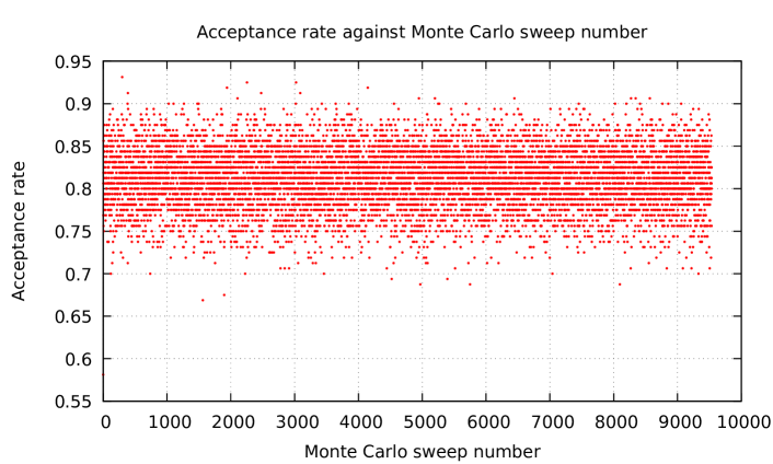
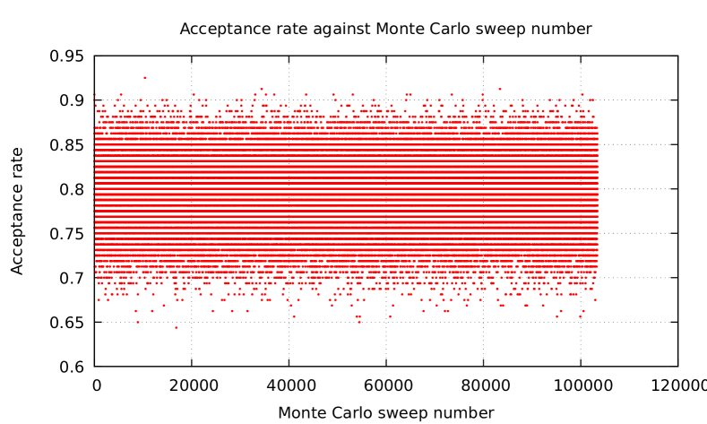
Let us discuss the initial conditions for the simulations first. For this model, we started our simulation with a cold start, i.e., all the field configurations are set to zero matrices. We also need to choose the value of the parameter δ𝛿\delta so that we get the acceptance rate between 65% and 85%. In Fig. 3.1 we show the acceptance rate for this simulation.

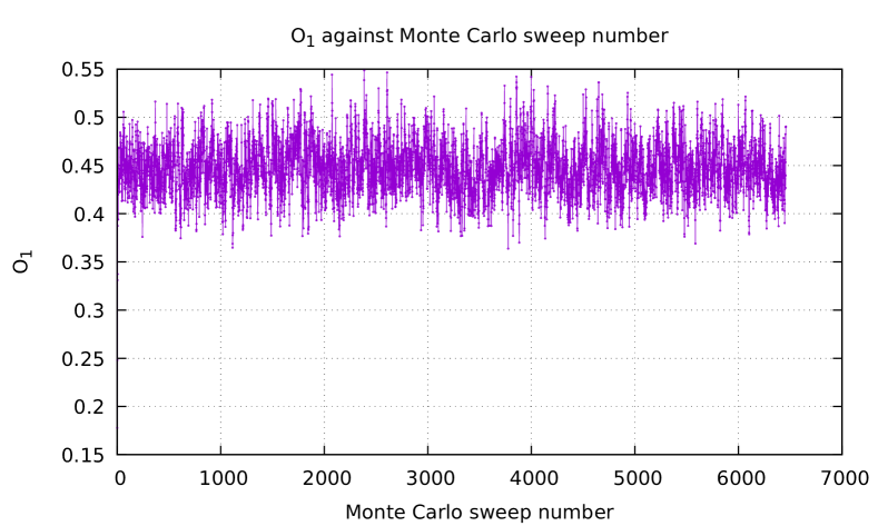
After that, we update the field configurations at a single lattice site for multiple times (in our case we updated field at each site 50 times) to make the system thermalize faster. We stored the value of the observables after every sweep. Now we need to decide whether the system has been thermalized or not. For that what we do is to simulate the system for large number of sweeps, say 10000. Then we plot one of the observables against the number of sweeps to see whether the system has been thermalized or not. When the value of the observable starts to oscillate about some value, then we are sure that the system has been thermalized. Let us look at the run time history of the observable O1subscript𝑂1O_{1} defined as

O11N2β0β𝑑tTr(X2)=1N2Tt=1TTr(Xt2)(Discretized version).formulae-sequencesubscript𝑂11superscript𝑁2𝛽superscriptsubscript0𝛽differential-d𝑡tracesuperscript𝑋21superscript𝑁2𝑇superscriptsubscript𝑡1𝑇tracesuperscriptsubscript𝑋𝑡2(Discretized version)\displaystyle O_{1}\equiv\frac{1}{N^{2}\beta}\int\limits_{0}^{\beta}dt\,\,\Tr(X^{2})=\frac{1}{N^{2}T}\sum\limits_{t=1}^{T}\Tr(X_{t}^{2})\qquad\textrm{(Discretized version)}. (3.7)

Now we collected the data for this observable after the system has been thermalized. We can see in Fig. 3.2 that the value of O1subscript𝑂1O_{1} is oscillating about 0.45. This observation leads us to the conclusion that the system has been thermalized and now we can collect the data for our calculation purpose.
Refer to caption
Figure 3.1: Acceptance rate against Monte Carlo sweep number. We can see that most of the values of the acceptance rate lies between 70% and 85%, which is good enough to get the desired results.
Refer to caption
Figure 3.2: Run-time history of observable O1subscript𝑂1O_{1} against Monte Carlo sweep number. Here we only plotted the run-time history after the system has been thermalized and discarded all the previous values. We can clearly see that the value of the observable O1subscript𝑂1O_{1} is oscillating around 0.45.

3.2.2 Autocorrelation

After thermalization, we collected data for the calculation purpose. It is clear from Fig. 3.2 that the value of O1subscript𝑂1O_{1} after every sweep is not statistically independent and it takes multiple sweeps to get a statistically independent value of the observable. We use the autocorrelation to get to know after how many sweeps the value of the observable are statistically independent.

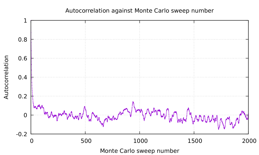
Fig. 3.3 shows the plot of normalized autocorrelation of the observable O1subscript𝑂1O_{1}. We can see that the plot decreases exponentially and after that, it just oscillates about zero. The point where the plot crosses the zero in the graph, we defined that thing as the autocorrelation length. So from this autocorrelation plot, we can see that the autocorrelation length for observable O1subscript𝑂1O_{1} is 158. Autocorrelation is an observable dependent quantity. It will be different for other observables. Hence the autocorrelation length will also be different for other observables.

For calculating any expectation value using Eq. 2.18, we need to take a gap of at least the autocorrelation length so that we only take the average of the uncorrelated data.
Refer to caption
Figure 3.3: Normalized autocorrelation against Monte Carlo sweep number for observable O1subscript𝑂1O_{1}. It starts from 1 and decreases exponentially towards 0 and then oscillates about 0. It crosses 0 value after 158 sweeps, so the autocorrelation length is 158 for O1subscript𝑂1O_{1}.

3.2.3 Two-point Correlation Function

One of the observables which we want to look at is the two-point correlation function. It is defined as

O2(t)1N2Tr(X(0)X(t))=1N2Tr(X0Xt)(Discretized form).formulae-sequencesubscript𝑂2𝑡1superscript𝑁2trace𝑋0𝑋𝑡1superscript𝑁2tracesubscript𝑋0subscript𝑋𝑡(Discretized form)\displaystyle O_{2}(t)\equiv\frac{1}{N^{2}}\Tr(X(0)X(t))=\frac{1}{N^{2}}\Tr(X_{0}X_{t})\qquad\textrm{(Discretized form)}. (3.8)

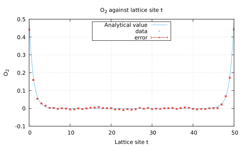
The theoretical result for the expectation value of O2subscript𝑂2O_{2} is

O2(t)=emt+em(βt)2m(1eβm).delimited-⟨⟩subscript𝑂2𝑡superscript𝑒𝑚𝑡superscript𝑒𝑚𝛽𝑡2𝑚1superscript𝑒𝛽𝑚\displaystyle\left\langle O_{2}(t)\right\rangle=\frac{e^{-mt}+e^{-m(\beta-t)}}{2m(1-e^{-\beta m})}. (3.9)

Fig. 3.4 shows the simulated result along with the theoretical result. We can see that it matches the theoretical result at most of the points but at some points it lies inside the error range. This result is convincing enough to believe that the algorithm is in working order.
Refer to caption
Figure 3.4: O2(t)delimited-⟨⟩subscript𝑂2𝑡\left\langle O_{2}(t)\right\rangle against lattice site t𝑡t. We simulated this on a lattice with 50 sites with lattice spacing a=1𝑎1a=1. We can see that the simulated result agrees with the theoretical result.

3.3 HMC for Harmonic Oscillator with Commutator Potential

Now we introduce more complexity into the harmonic oscillator potential by adding a commutator square term into the action. The Euclidean action is given by

SE=N2λ0β𝑑tTr[Xi˙2i,j=1i<jd[Xi,Xj]2+m2Xi2],subscript𝑆𝐸𝑁2𝜆superscriptsubscript0𝛽differential-d𝑡tracesuperscript˙superscript𝑋𝑖2superscriptsubscript𝑖𝑗1𝑖𝑗𝑑superscriptsuperscript𝑋𝑖superscript𝑋𝑗2superscript𝑚2superscriptsuperscript𝑋𝑖2\displaystyle S_{E}=\frac{N}{2\lambda}\int\limits_{0}^{\beta}\,dt\,\Tr\left[{\dot{X^{i}}}^{2}-\sum\limits_{\begin{subarray}{c}i,j=1\\ i<j\end{subarray}}^{d}[X^{i},X^{j}]^{2}+m^{2}{X^{i}}^{2}\right], (3.10)

where i,j𝑖𝑗i,j varies from 1 to d𝑑d, Xisuperscript𝑋𝑖X^{i} are N×N𝑁𝑁N\times N Hermitian matrices, λ𝜆\lambda is the ’t Hooft coupling defined as λ=NgYM2𝜆𝑁superscriptsubscript𝑔YM2\lambda=Ng_{\rm YM}^{2} where gYMsubscript𝑔YMg_{\rm YM} is the one-dimensional Yang-Mills coupling, m𝑚m is the mass. We are also using Einstein’s summation convention that the repeated indices are summed over. In the above d𝑑d is the number of spatial dimensions we want in our system. Right now we are just studying how to implement the algorithm properly so we stick to three spatial dimensions for this simulation. That is, d=3𝑑3d=3 in our simulations. (Note that this theory can be considered as the one obtained by dimensional reduction of a four-dimensional mother theory down to one dimension.)

Ideally, we need to simulate this model without mass term, but the model possesses flat directions. If we have a commutator potential square term Tr([Xi,Xj]2)tracesuperscriptsuperscript𝑋𝑖superscript𝑋𝑗2\Tr([X^{i},X^{j}]^{2}) then the system has flat directions associated with it [Joseph 15]. Flat directions are those field configurations which mutually commute with each other, i.e., [Xi,Xj]=0superscript𝑋𝑖superscript𝑋𝑗0[X^{i},X^{j}]=0 but the value of Tr(Xi2)tracesuperscriptsubscript𝑋𝑖2\Tr(X_{i}^{2}) keeps on increasing without an upper bound. This makes the simulation unstable, and we need to remove this to get the appropriate results. We can remove the flat directions in two ways. One way is to set the zero mode of the system. This is done by setting the global trace of the fields to zero.

t=1TTr(Xti)=0for each i.superscriptsubscript𝑡1𝑇tracesuperscriptsubscript𝑋𝑡𝑖0for each i\displaystyle\sum\limits_{t=1}^{T}\Tr(X_{t}^{i})=0\qquad\textrm{for each $i$}. (3.11)

But for simulations it is much easier to set the local trace to zero i.e., Tr(Xti)=0tracesuperscriptsubscript𝑋𝑡𝑖0\Tr(X_{t}^{i})=0 for each t𝑡t and i𝑖i. This will automatically satisfy the global trace condition Eq. (3.11).

Another way is to add a mass term in the Euclidean action itself as we have added in Eq. (3.10). Then we simulate the model for different mass values and extrapolate it towards zero mass limit to get the value of the observable at zero-mass value. We will simulate this model by applying both the methods to remove the flat directions and compare the extrapolated results with the exact zero-mass result.

Using the discretization procedure mentioned in Eqs. (2.4) - (2.7), the Euclidean action becomes

Slat=Na2λt=1TTr[(XtiXt1ia)2i,j=1i<jd[Xti,Xtj]2+m2Xti2]subscript𝑆lat𝑁𝑎2𝜆superscriptsubscript𝑡1𝑇tracesuperscriptsuperscriptsubscript𝑋𝑡𝑖superscriptsubscript𝑋𝑡1𝑖𝑎2superscriptsubscript𝑖𝑗1𝑖𝑗𝑑superscriptsuperscriptsubscript𝑋𝑡𝑖superscriptsubscript𝑋𝑡𝑗2superscript𝑚2superscriptsuperscriptsubscript𝑋𝑡𝑖2\displaystyle S_{\rm lat}=\frac{Na}{2\lambda}\sum\limits_{t=1}^{T}\,\,\Tr\left[\left(\frac{X_{t}^{i}-X_{t-1}^{i}}{a}\right)^{2}-\sum\limits_{\begin{subarray}{c}i,j=1\\ i<j\end{subarray}}^{d}[X_{t}^{i},X_{t}^{j}]^{2}+m^{2}{X_{t}^{i}}^{2}\right] (3.12)

with X0i=XTisuperscriptsubscript𝑋0𝑖superscriptsubscript𝑋𝑇𝑖X_{0}^{i}=X_{T}^{i}.

Now we need to setup the HMC algorithm for this model. First we need to introduce the momentum variable for each field variable Xtisuperscriptsubscript𝑋𝑡𝑖X_{t}^{i}. We introduce the momentum matrix Ptisuperscriptsubscript𝑃𝑡𝑖P_{t}^{i} for each Xtisuperscriptsubscript𝑋𝑡𝑖X_{t}^{i} matrix. Note that both Xtisuperscriptsubscript𝑋𝑡𝑖X_{t}^{i} and Ptisuperscriptsubscript𝑃𝑡𝑖P_{t}^{i} are Hermitian matrices. Now we introduce the Hamiltonian for this system. The Hamiltonian for this system is given by

H=𝐻absent\displaystyle H= t=1T12Tr(Pti2)+Slat,superscriptsubscript𝑡1𝑇12tracesuperscriptsuperscriptsubscript𝑃𝑡𝑖2subscript𝑆lat\displaystyle\sum\limits_{t=1}^{T}\frac{1}{2}\Tr({P_{t}^{i}}^{2})+S_{\rm lat}, (3.13)
H=𝐻absent\displaystyle H= t=1TTr[12Pti2+Na2λ{(XtiXt1ia)2i,j=1i<jd[Xti,Xtj]2+m2Xti2}].superscriptsubscript𝑡1𝑇trace12superscriptsuperscriptsubscript𝑃𝑡𝑖2𝑁𝑎2𝜆superscriptsuperscriptsubscript𝑋𝑡𝑖superscriptsubscript𝑋𝑡1𝑖𝑎2superscriptsubscript𝑖𝑗1𝑖𝑗𝑑superscriptsuperscriptsubscript𝑋𝑡𝑖superscriptsubscript𝑋𝑡𝑗2superscript𝑚2superscriptsuperscriptsubscript𝑋𝑡𝑖2\displaystyle\sum\limits_{t=1}^{T}\Tr\left[\frac{1}{2}{P_{t}^{i}}^{2}+\frac{Na}{2\lambda}\left\{\left(\frac{X_{t}^{i}-X_{t-1}^{i}}{a}\right)^{2}-\sum\limits_{\begin{subarray}{c}i,j=1\\ i<j\end{subarray}}^{d}[X_{t}^{i},X_{t}^{j}]^{2}+m^{2}{X_{t}^{i}}^{2}\right\}\right]. (3.14)

Our next task is to set the initial conditions for the field variables and take the momentum value randomly from the 𝒩(0,1)𝒩01\mathcal{N}(0,1) distribution. Details about how to generate random numbers distributed as Gaussian distribution can be found in Ref. [Ydri 17]. After that we need to evolve the field and momentum variables according to the Hamilton’s equations.

We need to find the forces for each momentum variable. We have

(Xti˙)rs=H(Pti)srand(Pti˙)rs=H(Xti)sr,formulae-sequencesubscript˙superscriptsubscript𝑋𝑡𝑖𝑟𝑠𝐻subscriptsuperscriptsubscript𝑃𝑡𝑖𝑠𝑟andsubscript˙superscriptsubscript𝑃𝑡𝑖𝑟𝑠𝐻subscriptsuperscriptsubscript𝑋𝑡𝑖𝑠𝑟(\dot{X_{t}^{i}})_{rs}=\frac{\partial H}{\partial(P_{t}^{i})_{sr}}\hskip 14.22636pt{\rm and}\hskip 14.22636pt(\dot{P_{t}^{i}})_{rs}=-\frac{\partial H}{\partial(X_{t}^{i})_{sr}}, (3.15)

where the dot on the field and momentum variables are time derivatives with respect to the fictitious time τ𝜏\tau. We then have the equation of motion

(Xti˙)rssubscript˙superscriptsubscript𝑋𝑡𝑖𝑟𝑠\displaystyle(\dot{X_{t}^{i}})_{rs} =\displaystyle= (Pti)rs,subscriptsuperscriptsubscript𝑃𝑡𝑖𝑟𝑠\displaystyle(P_{t}^{i})_{rs}, (3.16)
(Pti˙)rssubscript˙superscriptsubscript𝑃𝑡𝑖𝑟𝑠\displaystyle(\dot{P_{t}^{i}})_{rs} =\displaystyle= Naλ[(2a2+m2)(Xti)rs1a2[(Xt1i)rs+(Xt+1i)rs]\displaystyle-\frac{Na}{\lambda}\Bigg{[}\left(\frac{2}{a^{2}}+m^{2}\right){(X_{t}^{i})}_{rs}-\frac{1}{a^{2}}\left[{(X_{t-1}^{i})}_{rs}+{(X_{t+1}^{i})}_{rs}\right] (3.17)
j=1jid[Xtj,[Xti,Xtj]]rs].\displaystyle\hskip 56.9055pt-\sum\limits_{\begin{subarray}{c}j=1\\ j\neq i\end{subarray}}^{d}[X_{t}^{j},[X_{t}^{i},X_{t}^{j}]]_{rs}\Bigg{]}.

In matrix form these equations simply become

Xti˙=˙superscriptsubscript𝑋𝑡𝑖absent\displaystyle\dot{X_{t}^{i}}= Pti,superscriptsubscript𝑃𝑡𝑖\displaystyle P_{t}^{i}, (3.18)
Pti˙=˙superscriptsubscript𝑃𝑡𝑖absent\displaystyle\dot{P_{t}^{i}}= Naλ[(2a2+m2)Xti1a2(Xt1i+Xt+1i)j=1jid[Xtj,[Xti,Xtj]]].𝑁𝑎𝜆delimited-[]2superscript𝑎2superscript𝑚2superscriptsubscript𝑋𝑡𝑖1superscript𝑎2superscriptsubscript𝑋𝑡1𝑖superscriptsubscript𝑋𝑡1𝑖superscriptsubscript𝑗1𝑗𝑖𝑑superscriptsubscript𝑋𝑡𝑗superscriptsubscript𝑋𝑡𝑖superscriptsubscript𝑋𝑡𝑗\displaystyle-\frac{Na}{\lambda}\Bigg{[}\left(\frac{2}{a^{2}}+m^{2}\right)X_{t}^{i}-\frac{1}{a^{2}}\left(X_{t-1}^{i}+X_{t+1}^{i}\right)-\sum\limits_{\begin{subarray}{c}j=1\\ j\neq i\end{subarray}}^{d}[X_{t}^{j},[X_{t}^{i},X_{t}^{j}]]\Bigg{]}. (3.19)

We will evolve the above equations using the leapfrog algorithm described in the previous chapter, Eq. (2.25) - (2.27). The equations are simply

Pti(τ+ϵ2)superscriptsubscript𝑃𝑡𝑖𝜏italic-ϵ2\displaystyle P_{t}^{i}\left(\tau+\frac{\epsilon}{2}\right) =Pti(τ)ϵ2HXti(Xt(τ)),absentsuperscriptsubscript𝑃𝑡𝑖𝜏italic-ϵ2𝐻superscriptsubscript𝑋𝑡𝑖subscript𝑋𝑡𝜏\displaystyle=P_{t}^{i}(\tau)-\frac{\epsilon}{2}\frac{\partial H}{\partial X_{t}^{i}}(X_{t}(\tau)), (3.20)
Xti(τ+ϵ)superscriptsubscript𝑋𝑡𝑖𝜏italic-ϵ\displaystyle X_{t}^{i}(\tau+\epsilon) =Xti(τ)+ϵPti(τ+ϵ2),absentsuperscriptsubscript𝑋𝑡𝑖𝜏italic-ϵsuperscriptsubscript𝑃𝑡𝑖𝜏italic-ϵ2\displaystyle=X_{t}^{i}(\tau)+\epsilon P_{t}^{i}\left(\tau+\frac{\epsilon}{2}\right), (3.21)
Pti(τ+ϵ)superscriptsubscript𝑃𝑡𝑖𝜏italic-ϵ\displaystyle P_{t}^{i}(\tau+\epsilon) =Pti(τ+ϵ2)ϵ2HXti(Xt(τ+ϵ)),absentsuperscriptsubscript𝑃𝑡𝑖𝜏italic-ϵ2italic-ϵ2𝐻superscriptsubscript𝑋𝑡𝑖subscript𝑋𝑡𝜏italic-ϵ\displaystyle=P_{t}^{i}\left(\tau+\frac{\epsilon}{2}\right)-\frac{\epsilon}{2}\frac{\partial H}{\partial X_{t}^{i}}(X_{t}(\tau+\epsilon)), (3.22)

where ϵitalic-ϵ\epsilon is a tunable parameter. We also have one more tunable parameter here which is the number of times we evolve the fields using the leapfrog algorithm. We call this parameter n𝑛n. So we evolve the fields for n𝑛n times and for nϵ𝑛italic-ϵn\epsilon amount of fictitious time. Both ϵitalic-ϵ\epsilon and n𝑛n must be tuned to get the desirable acceptance rate in the simulations.

After evolving the fields and their conjugate momenta, we need to compare it with the initial field and their momenta. For that, we need to calculate the acceptance probability for this algorithm. Acceptance probability for this algorithm is simply eΔH=exp((H(Xi(nϵ),Pi(nϵ))H(Xi(0),Pi(0))))superscript𝑒Δ𝐻𝐻superscript𝑋𝑖𝑛italic-ϵsuperscript𝑃𝑖𝑛italic-ϵ𝐻superscript𝑋𝑖0superscript𝑃𝑖0e^{-\Delta H}=\exp{-(H(X^{i}(n\epsilon),P^{i}(n\epsilon))-H(X^{i}(0),P^{i}(0)))}. We accept the proposed state with the probability eΔHsuperscript𝑒Δ𝐻e^{-\Delta H}. For that, we take a random number α𝛼\alpha from a uniform random number distribution between (0,1)01(0,1). If αeΔH𝛼superscript𝑒Δ𝐻\alpha\leq e^{-\Delta H}, then we accept the proposed state, otherwise we reject the proposed state and propose a new state and continue this procedure until we have enough data to calculate the expectation value of the observable.

For this algorithm also we require the acceptance rate between 65-85% to move through the configuration space optimally. This acceptance rate can be achieved by tuning ϵitalic-ϵ\epsilon and n𝑛n parameters appropriately.

3.4 Simulation Details and Results

Similar to the Metropolis algorithm, we need to monitor some of the important things for the HMC algorithm also. We will discuss these in this section and later will show some results for this model.

In this simulation each variable and parameter has been measured in the unit of ’t Hooft coupling λ0subscript𝜆0\lambda_{0}. Since the Yang-Mills coupling gYM2superscriptsubscript𝑔YM2g_{\rm YM}^{2} has a dimension of [L3superscript𝐿3L^{-3}] in one dimension, so X𝑋X can be measured in the unit of λ01/3superscriptsubscript𝜆013\lambda_{0}^{1/3}, a𝑎a can be measured in units of λ01/3superscriptsubscript𝜆013\lambda_{0}^{-1/3} and mass m𝑚m can be measured in units of λ01/3superscriptsubscript𝜆013\lambda_{0}^{1/3}. Thus, every variable and parameter appearing in Eq. (3.10) are dimensionless. Values of the parameter used for this simulations are: N=8𝑁8N=8, a=0.5𝑎0.5a=0.5, T=10𝑇10T=10, β=5𝛽5\beta=5, d=3𝑑3d=3 and λ=1𝜆1\lambda=1. We have taken m=0.01𝑚0.01m=0.01 for the results of the next two sub-sections.

3.4.1 Initial Conditions, Acceptance Rate and Thermalization

We started the simulation with a cold start, i.e., all the field configurations are set to zero matrices initially. To explore the configuration space more efficiently, we choose our tunable parameter ϵitalic-ϵ\epsilon and n𝑛n so that we get the acceptance rate between 65-85%. Fig. 3.5 shows the acceptance rate against Monte Carlo sweeps for this simulation. Tuning these parameters is a very crucial step for the HMC algorithm. Sometimes a slight change in these parameters can make the simulation unstable.

After tuning these parameters, we monitor the quantity eΔHsuperscript𝑒Δ𝐻e^{-\Delta H}. As mentioned in the previous chapter, this is one of the tests to check whether the HMC has been implemented properly or not. Fig. 3.6 shows the plot of eΔHsuperscript𝑒Δ𝐻e^{-\Delta H} against number of accepted states. We can clearly see that the data points oscillate about 1 in this plot. The average value of the eΔHsuperscript𝑒Δ𝐻e^{-\Delta H} comes out to be 1.10195±0.29467plus-or-minus1.101950.294671.10195\pm 0.29467, which clearly shows that the expected value, 1, lies within the error range. This is enough to show that the algorithm is working fine.

Since this is also a Monte Carlo simulation and uses Markov chain to converge to the desired distribution so we will expect that the value of the observable first start from some value and after some sweeps it will thermalize and then oscillate about some value. The feature appears here also but the system thermalizes much faster for this algorithm as compared to the Metropolis algorithm. In Fig. 3.7 we show Monte Carlo time history of the observable O3subscript𝑂3O_{3} defined as

O31Nβ0β𝑑tTr(Xi2)=1NTt=1TTr(Xti2)(Discretized form).formulae-sequencesubscript𝑂31𝑁𝛽superscriptsubscript0𝛽differential-d𝑡tracesuperscriptsuperscript𝑋𝑖21𝑁𝑇superscriptsubscript𝑡1𝑇tracesuperscriptsuperscriptsubscript𝑋𝑡𝑖2(Discretized form)\displaystyle O_{3}\equiv\frac{1}{N\beta}\int\limits_{0}^{\beta}dt\,\,\Tr({X^{i}}^{2})=\frac{1}{NT}\sum\limits_{t=1}^{T}\Tr({X_{t}^{i}}^{2})\qquad\textrm{(Discretized form)}. (3.23)
Refer to caption
Figure 3.5: Acceptance rate against Monte Carlo sweep number. We can see that most of the data points are concentrated between 75 to 85%, which is what we want for good simulation results.
Refer to caption
Figure 3.6: The plot of eΔHsuperscript𝑒Δ𝐻e^{-\Delta H} against the number of accepted states. In this plot we can see that most of the values are concentrated near 1 which is a clear indication that HMC algorithm has been implemented correctly.
Refer to caption
Figure 3.7: Run-time history of observable O3subscript𝑂3O_{3} against Monte Carlo sweep number. The data tell us that it took only about 10-12 sweeps for the system to thermalize.

3.4.2 Autocorrelation

Looking at the plot of the run-time history of the observable O3subscript𝑂3O_{3}, it is clear that the data points are correlated with each other, and we need to skip a certain number of consecutive steps to get uncorrelated data. Fig. 3.8 shows the plot of normalized autocorrelation against the number of sweeps for the observable O3subscript𝑂3O_{3}. Autocorrelation quickly decays and oscillate about zero after about 15-16 sweeps, which shows that the autocorrelation between the data points is quite less. Autocorrelation length of this observable comes out to be 15.
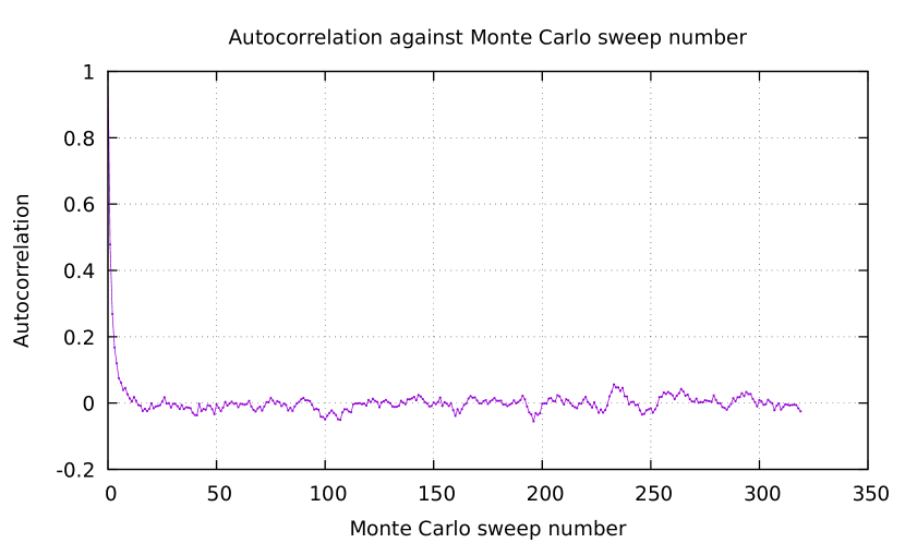
Refer to caption
Figure 3.8: Normalized autocorrelation against Monte Carlo sweep number. If we compare it with Fig. 3.3 we see that the data obtained through HMC algorithm are not that correlated compared to the data obtained through the Metropolis algorithm.

3.4.3 Result

We simulated this model by removing the flat directions in two ways. First, we simulated the model at m=0𝑚0m=0 by applying the local trace condition. We calculated the value of the observable O3subscript𝑂3O_{3} from this simulation. Then we simulated this model by adding different mass terms and then linearly extrapolated it towards zero mass limit. Table 3.1 shows the value of O3subscript𝑂3O_{3} for different mass m𝑚m. Fig. 3.9 shows the plot of O3subscript𝑂3O_{3} against mass m𝑚m. The straight line is the linear fit to the data.

m𝑚m O3subscript𝑂3O_{3}
0.0 1.34458(303)
0.01 1.34794(315)
0.1 1.33892(291)
0.5 1.24151(258)
1.0 1.02051(145)
1.5 0.81008(106)
2.0 0.63752(81)
Table 3.1: The value of observable O3subscript𝑂3O_{3} for different m𝑚m values.
Refer to caption
Figure 3.9: The observable O3subscript𝑂3O_{3} against m𝑚m. The plot also contains the linear fit to the data.

Equation of the linear fit is given by

O3=0.3630(151)m+1.3709(156).subscript𝑂30.3630151𝑚1.3709156\displaystyle O_{3}=-0.3630(151)~{}m+1.3709(156). (3.24)

From the linear fit we get the value of O3subscript𝑂3O_{3} at m=0𝑚0m=0 to be 1.3709(156)1.37091561.3709(156), which clearly differs from the simulation at m=0𝑚0m=0 case given in Table 3.1. This may be because the linear extrapolation is only the first-order correction and we need to know how the observable behaves for different mass values. If we have some idea on how the observable behaves with different mass, then we can use that information for extrapolation.

3.5 Remarks

In this chapter, we simulated two different models, harmonic oscillator and harmonic oscillator with commutator potential, using two different algorithms. The second model is more complicated as compared to the first one. We have observed that using HMC algorithm on the second model not only made the system to thermalize much faster but also the autocorrelation between the data is quite less as compared to the simulation done using the Metropolis algorithm. Although we have not simulated the same model with both the algorithms but the second model is more complicated as compared to the first one. So from here, we conclude that HMC algorithm is more efficient as compared to the Metropolis algorithm. From the next chapter onwards, we will use the HMC algorithm for the simulations.

Chapter 4 Bosonic D=4𝐷4D=4 and BFSS Matrix Models

In this chapter, we are first going to discuss how to implement gauge fields on the lattice and then apply these techniques to simulate the bosonic D=4𝐷4D=4 and bosonic BFSS models. Simulations including fermions will be discussed in the next chapter.

4.1 Gauge Theory on a Lattice

Most of the contents of this section can be found in Ref. [Gattringer 09]. They have performed these calculations for lattice QCD but we will do it for more general gauge group SU(N)𝑆𝑈𝑁SU(N).

In this section we try to describe how to implement gauge fields on a lattice by using an example of Yang-Mills theory coupled to a complex scalar field in four spacetime dimensions. We take the gauge group of the gauge field to be SU(N)𝑆𝑈𝑁SU(N). The scalar field transforms in the fundamental representation of this gauge group. The metric of the four-dimensional spacetime is ημν=diag(1,1,1,1)subscript𝜂𝜇𝜈diag1111\eta_{\mu\nu}={\rm diag}(1,-1,-1,-1).

The action of this theory is given by

S=d4x{12g2Tr(FμνFμν)+(DμΦ)DμΦm2ΦΦ},𝑆superscript𝑑4𝑥12superscript𝑔2tracesubscript𝐹𝜇𝜈superscript𝐹𝜇𝜈superscriptsubscript𝐷𝜇Φsuperscript𝐷𝜇Φsuperscript𝑚2superscriptΦΦS=\int d^{4}x\left\{-\frac{1}{2g^{2}}\Tr(F_{\mu\nu}F^{\mu\nu})+{(D_{\mu}\Phi)}^{\dagger}D^{\mu}\Phi-m^{2}\Phi^{\dagger}\Phi\right\}, (4.1)

where

Dμsubscript𝐷𝜇\displaystyle D_{\mu} =\displaystyle= μ+iAμ,subscript𝜇𝑖subscript𝐴𝜇\displaystyle\partial_{\mu}+iA_{\mu}, (4.2)
Fμνsubscript𝐹𝜇𝜈\displaystyle F_{\mu\nu} =\displaystyle= [μAν]+i[Aμ,Aν].\displaystyle\partial_{[\mu}A_{\nu]}+i[A_{\mu},A_{\nu}]. (4.3)

The path integral for this model is given by

Z=𝒟Aμ𝒟Φexp(iS).𝑍𝒟subscript𝐴𝜇𝒟Φ𝑖𝑆Z=\int\mathcal{D}A_{\mu}\,\,\mathcal{D}\Phi\,\,\exp{iS}. (4.4)

After performing the Wick rotation we will get the Euclidean action for this model. The details of this is given in Appendix A. The metric after Wick rotation becomes ημν=diag(1,1,1,1)subscript𝜂𝜇𝜈diag1111\eta_{\mu\nu}={\rm diag}(1,1,1,1). The Euclidean action is given by

SE=d4xE{12g2Tr(Fμν2)E+(DμΦ)DμΦ+m2ΦΦ},subscript𝑆𝐸superscript𝑑4subscript𝑥𝐸12superscript𝑔2subscripttracesuperscriptsubscript𝐹𝜇𝜈2𝐸superscriptsubscript𝐷𝜇Φsubscript𝐷𝜇Φsuperscript𝑚2superscriptΦΦ\displaystyle S_{E}=\int d^{4}x_{E}\,\,\left\{\frac{1}{2g^{2}}\Tr(F_{\mu\nu}^{2})_{E}+{(D_{\mu}\Phi)}^{\dagger}D_{\mu}\Phi+m^{2}{\Phi}^{\dagger}\Phi\right\}, (4.5)

where

FμνEsubscriptsubscript𝐹𝜇𝜈𝐸\displaystyle{F_{\mu\nu}}_{E} =\displaystyle= [μAν]+i[Aμ,Aν],\displaystyle\partial_{[\mu}A_{\nu]}+i[A_{\mu},A_{\nu}], (4.6)
Dμsubscript𝐷𝜇\displaystyle D_{\mu} =\displaystyle= μ+iAμ.subscript𝜇𝑖subscript𝐴𝜇\displaystyle\partial_{\mu}+iA_{\mu}. (4.7)

While working in Euclidean spacetime we note that we do not need to change the sign when we go from lower index to upper index and vice-versa. Let us represent all tensor quantities using only the lower indices. Another item that has changed is that now both μ𝜇\mu and ν𝜈\nu will run from 1 to 4 instead of 0 to 3. As both the fields are bosonic type they will satisfy periodic boundary conditions in Euclidean time tEsubscript𝑡𝐸t_{E}, i.e.,

A(x,tE+β)𝐴𝑥subscript𝑡𝐸𝛽\displaystyle A(\vec{x},t_{E}+\beta) =\displaystyle= A(x,tE),𝐴𝑥subscript𝑡𝐸\displaystyle A(\vec{x},t_{E}), (4.8)
Φ(x,tE+β)Φ𝑥subscript𝑡𝐸𝛽\displaystyle\Phi(\vec{x},t_{E}+\beta) =\displaystyle= Φ(x,tE).Φ𝑥subscript𝑡𝐸\displaystyle\Phi(\vec{x},t_{E}). (4.9)

From now on we will suppress the subscript E𝐸E on the expressions and we will get to know the distinction between the Euclidean and Minkowski terms from the context.

Now we can discretize the above action to put the theory on the lattice. We cannot discretize this theory using a naive lattice discretization as this theory is locally gauge invariant under the gauge transformation

Φ(x)Φ𝑥\displaystyle\Phi(x) \displaystyle\longrightarrow V(x)Φ(x),𝑉𝑥Φ𝑥\displaystyle V(x)\Phi(x), (4.10)
Aμ(x)subscript𝐴𝜇𝑥\displaystyle A_{\mu}(x) \displaystyle\longrightarrow V(x)Aμ(x)V(x)+iμV(x)V(x).𝑉𝑥subscript𝐴𝜇𝑥superscript𝑉𝑥𝑖subscript𝜇𝑉𝑥superscript𝑉𝑥\displaystyle V(x)A_{\mu}(x)V^{\dagger}(x)+i\partial_{\mu}V(x)V^{\dagger}(x). (4.11)

In the above equations we have V(x)=exp(iΛ(x))𝑉𝑥𝑖Λ𝑥V(x)=\exp(-i\Lambda(x)) with Λ(x)Λ𝑥\Lambda(x) belonging to the Lie algebra 𝔰𝔲(N)𝔰𝔲𝑁\mathfrak{su}(N), x4𝑥superscript4x\in\mathbb{R}^{4} and V(x)=V1(x)superscript𝑉𝑥superscript𝑉1𝑥V^{\dagger}(x)=V^{-1}(x).

Our aim is to make the lattice action locally gauge invariant such that in the limit of lattice spacing a𝑎a going to zero we get back the action of the continuum theory. To do this let us first forget about the gauge field for now and focus on the free scalar field whose Euclidean action is given by

S=d4x{μΦμΦ+m2ΦΦ}.𝑆superscript𝑑4𝑥subscript𝜇superscriptΦsubscript𝜇Φsuperscript𝑚2superscriptΦΦS=\int d^{4}x\left\{\partial_{\mu}\Phi^{\dagger}\partial_{\mu}\Phi+m^{2}\Phi^{\dagger}\Phi\right\}. (4.12)

As no gauge field is present we can simply discretize the action to get the lattice action

Slat=a4nΛ[μ=14(Φn+μ^Φn)(Φn+μ^Φn)a2+m2ΦnΦn],subscript𝑆latsuperscript𝑎4subscript𝑛Λdelimited-[]superscriptsubscript𝜇14superscriptsubscriptΦ𝑛^𝜇superscriptsubscriptΦ𝑛subscriptΦ𝑛^𝜇subscriptΦ𝑛superscript𝑎2superscript𝑚2superscriptsubscriptΦ𝑛subscriptΦ𝑛\displaystyle S_{\rm lat}=a^{4}\sum\limits_{n\in\Lambda}\left[\sum\limits_{\mu=1}^{4}\frac{\left(\Phi_{n+\hat{\mu}}^{\dagger}-\Phi_{n}^{\dagger}\right)\left(\Phi_{n+\hat{\mu}}-\Phi_{n}\right)}{a^{2}}+m^{2}\Phi_{n}^{\dagger}\Phi_{n}\right], (4.13)

where Λ={n=(n1,n2,n3,n4)|n1,n2,n3=1,2,,Ns;n4=1,2,,Tandx=na}Λconditional-set𝑛subscript𝑛1subscript𝑛2subscript𝑛3subscript𝑛4formulae-sequencesubscript𝑛1subscript𝑛2subscript𝑛312subscript𝑁𝑠subscript𝑛412𝑇and𝑥𝑛𝑎\Lambda=\left\{n=(n_{1},n_{2},n_{3},n_{4})|\,\,n_{1},n_{2},n_{3}=1,2,\cdots,N_{s};\,\,n_{4}=1,2,\cdots,T\,\,{\rm and}\,\,x=na\right\}, μ^^𝜇\hat{\mu} is the basis vector on the lattice; 1^=(1,0,0,0)^11000\hat{1}=(1,0,0,0) and similarly for 2^,3^^2^3\hat{2},\,\hat{3} and 4^^4\hat{4}. We also apply periodic boundary conditions in all the four directions. It is easy to see that the term ΦnΦnsuperscriptsubscriptΦ𝑛subscriptΦ𝑛\Phi_{n}^{\dagger}\Phi_{n} is gauge invariant as both of these belong to the same lattice point and the gauge transformation cancels each other leaving this term invariant. Now we need to check whether the term Φn+μ^ΦnsuperscriptsubscriptΦ𝑛^𝜇subscriptΦ𝑛\Phi_{n+\hat{\mu}}^{\dagger}\Phi_{n} remains invariant or not. We do the required calculation by transforming the field at both of these lattice points by appropriate transformations

ΦnsubscriptΦ𝑛\displaystyle\Phi_{n} \displaystyle\longrightarrow V(n)Φn,𝑉𝑛subscriptΦ𝑛\displaystyle V(n)\Phi_{n}, (4.14)
Φn+μ^superscriptsubscriptΦ𝑛^𝜇\displaystyle\Phi_{n+\hat{\mu}}^{\dagger} \displaystyle\longrightarrow Φn+μ^V(n+μ^),superscriptsubscriptΦ𝑛^𝜇superscript𝑉𝑛^𝜇\displaystyle\Phi_{n+\hat{\mu}}^{\dagger}V^{\dagger}(n+\hat{\mu}), (4.15)
Φn+μ^ΦnsuperscriptsubscriptΦ𝑛^𝜇subscriptΦ𝑛\displaystyle\Phi_{n+\hat{\mu}}^{\dagger}\Phi_{n} \displaystyle\longrightarrow Φn+μ^V(n+μ^)V(n)Φn,superscriptsubscriptΦ𝑛^𝜇superscript𝑉𝑛^𝜇𝑉𝑛subscriptΦ𝑛\displaystyle\Phi_{n+\hat{\mu}}^{\dagger}V^{\dagger}(n+\hat{\mu})V(n)\Phi_{n}, (4.16)

where both V(n+μ^)superscript𝑉𝑛^𝜇V^{\dagger}(n+\hat{\mu}) and V(n)𝑉𝑛V(n) belong to SU(N)𝑆𝑈𝑁SU(N). We note that V(n+μ^)𝑉𝑛^𝜇V(n+\hat{\mu}) and V(n)𝑉𝑛V(n) can be different in general. Thus the above term is not locally gauge invariant and this is the only term (and a complex conjugate term also) in the action Eq. (4.13) which is not locally gauge invariant. We need to add something in between Φn+μ^superscriptsubscriptΦ𝑛^𝜇\Phi_{n+\hat{\mu}}^{\dagger} and ΦnsubscriptΦ𝑛\Phi_{n} which cancels these gauge transformations. We know one such object which transforms in the opposite direction to that of the scalar field. It is the path ordering of the exponential of the line integral of gauge field along some curve γ𝛾\gamma connecting points from x𝑥x to y𝑦y. It is called the Wilson line integral or the gauge transporter. The expression of the operator and the transformation properties are given by

U(x,y)𝑈𝑥𝑦\displaystyle U(x,y) =\displaystyle= P{exp[iγ𝑑zμAμ(z)]},𝑃𝑖subscript𝛾differential-dsubscript𝑧𝜇subscript𝐴𝜇𝑧\displaystyle P\left\{\exp\left[i\int\limits_{\gamma}dz_{\mu}\,A_{\mu}(z)\right]\right\}, (4.17)
U(x,y)𝑈𝑥𝑦\displaystyle U(x,y) \displaystyle\longrightarrow V(x)U(x,y)V(y),𝑉𝑥𝑈𝑥𝑦superscript𝑉𝑦\displaystyle V(x)U(x,y)V^{\dagger}(y), (4.18)

where P𝑃P stands for path ordering. If we have an analog of this for the lattice then we can use that to make Φn+μ^ΦnsuperscriptsubscriptΦ𝑛^𝜇subscriptΦ𝑛\Phi_{n+\hat{\mu}}^{\dagger}\Phi_{n} locally gauge invariant. If we replace x𝑥x with n𝑛n and y𝑦y with n+μ^𝑛^𝜇n+\hat{\mu} and approximate the line integral with iaAμ(n)𝑖𝑎subscript𝐴𝜇𝑛iaA_{\mu}(n) then to the lowest order of approximation we do not need any path ordering and only higher order terms will have path ordering terms. Thus we get

U(n,n+μ^)𝑈𝑛𝑛^𝜇\displaystyle U(n,n+\hat{\mu}) =\displaystyle= exp(iaAμ(n))=Uμ(n),𝑖𝑎subscript𝐴𝜇𝑛subscript𝑈𝜇𝑛\displaystyle\exp{iaA_{\mu}(n)}=U_{\mu}(n), (4.19)
Uμ(n)subscript𝑈𝜇𝑛\displaystyle U_{\mu}(n) \displaystyle\longrightarrow V(n)Uμ(n)V(n+μ^).𝑉𝑛subscript𝑈𝜇𝑛superscript𝑉𝑛^𝜇\displaystyle V(n)U_{\mu}(n)V^{\dagger}(n+\hat{\mu}). (4.20)

This operator Uμ(n)subscript𝑈𝜇𝑛U_{\mu}(n) is known as the link field. Also note that Uμ(n)=U(n,nμ^)=exp(iaAμ(n))=Uμ(nμ^)subscript𝑈𝜇𝑛𝑈𝑛𝑛^𝜇𝑖𝑎subscript𝐴𝜇𝑛superscriptsubscript𝑈𝜇𝑛^𝜇U_{-\mu}(n)=U(n,n-\hat{\mu})=\exp{-iaA_{\mu}(n)}=U_{\mu}^{\dagger}(n-\hat{\mu}). We note that Uμ(n)subscript𝑈𝜇𝑛U_{\mu}(n) has a directional nature, i.e., Uμ(n)subscript𝑈𝜇𝑛U_{\mu}(n) connects n𝑛n to n+μ^𝑛^𝜇n+\hat{\mu} and Uμ(n)subscript𝑈𝜇𝑛U_{-\mu}(n) connects n𝑛n to nμ^𝑛^𝜇n-\hat{\mu}. So if we add U(n+μ^,n)=Uμ(n+μ^)=Uμ(n)𝑈𝑛^𝜇𝑛subscript𝑈𝜇𝑛^𝜇superscriptsubscript𝑈𝜇𝑛U(n+\hat{\mu},n)=U_{-\mu}(n+\hat{\mu})=U_{\mu}^{\dagger}(n) in between Φn+μ^superscriptsubscriptΦ𝑛^𝜇\Phi_{n+\hat{\mu}}^{\dagger} and ΦnsubscriptΦ𝑛\Phi_{n} we get Φn+μ^Uμ(n)ΦnsuperscriptsubscriptΦ𝑛^𝜇superscriptsubscript𝑈𝜇𝑛subscriptΦ𝑛\Phi_{n+\hat{\mu}}^{\dagger}U_{\mu}^{\dagger}(n)\Phi_{n}. We can easily check that it is locally gauge invariant. The calculations are provided below

Φn+μ^Uμ(n)ΦnΦn+μ^V(n+μ^)V(n+μ^)Uμ(n)V(n)V(n)Φn=Φn+μ^Uμ(n)Φn.superscriptsubscriptΦ𝑛^𝜇superscriptsubscript𝑈𝜇𝑛subscriptΦ𝑛superscriptsubscriptΦ𝑛^𝜇superscript𝑉𝑛^𝜇𝑉𝑛^𝜇superscriptsubscript𝑈𝜇𝑛superscript𝑉𝑛𝑉𝑛subscriptΦ𝑛superscriptsubscriptΦ𝑛^𝜇superscriptsubscript𝑈𝜇𝑛subscriptΦ𝑛\Phi_{n+\hat{\mu}}^{\dagger}U_{\mu}^{\dagger}(n)\Phi_{n}\longrightarrow\Phi_{n+\hat{\mu}}^{\dagger}V^{\dagger}(n+\hat{\mu})V(n+\hat{\mu})U_{\mu}^{\dagger}(n)V^{\dagger}(n)V(n)\Phi_{n}=\Phi_{n+\hat{\mu}}^{\dagger}U_{\mu}^{\dagger}(n)\Phi_{n}. (4.21)

Now we are left with our last task to check whether in the limit a0𝑎0a\longrightarrow 0 we get the correct continuum action or not. So let us insert the required link fields in the action Eq. (4.13) and take the limit a0𝑎0a\longrightarrow 0. This is done by first replacing Φn+μ^superscriptsubscriptΦ𝑛^𝜇\Phi_{n+\hat{\mu}}^{\dagger} with Φn+μ^Uμ(n)superscriptsubscriptΦ𝑛^𝜇superscriptsubscript𝑈𝜇𝑛\Phi_{n+\hat{\mu}}^{\dagger}U_{\mu}^{\dagger}(n). Then the action becomes

Ssc=a4nΛ[μ=14(Φn+μ^Uμ(n)Φn)(Uμ(n)Φn+μ^Φn)a2+m2ΦnΦn].subscript𝑆scsuperscript𝑎4subscript𝑛Λdelimited-[]superscriptsubscript𝜇14superscriptsubscriptΦ𝑛^𝜇superscriptsubscript𝑈𝜇𝑛superscriptsubscriptΦ𝑛subscript𝑈𝜇𝑛subscriptΦ𝑛^𝜇subscriptΦ𝑛superscript𝑎2superscript𝑚2superscriptsubscriptΦ𝑛subscriptΦ𝑛S_{\rm sc}=a^{4}\sum\limits_{n\in\Lambda}\left[\sum\limits_{\mu=1}^{4}\frac{\Big{(}\Phi_{n+\hat{\mu}}^{\dagger}U_{\mu}^{\dagger}(n)-\Phi_{n}^{\dagger}\Big{)}\Big{(}U_{\mu}(n)\Phi_{n+\hat{\mu}}-\Phi_{n}\Big{)}}{a^{2}}+m^{2}\Phi_{n}^{\dagger}\Phi_{n}\right]. (4.22)

From Eq. (4.19) it is clear that Uμ(n)=𝟙+iaAμ(n)+𝒪(a2)subscript𝑈𝜇𝑛1𝑖𝑎subscript𝐴𝜇𝑛𝒪superscript𝑎2U_{\mu}(n)=\mathbb{1}+iaA_{\mu}(n)+\mathcal{O}(a^{2}) and Uμ(n)=𝟙iaAμ(n)+𝒪(a2)superscriptsubscript𝑈𝜇𝑛1𝑖𝑎subscript𝐴𝜇𝑛𝒪superscript𝑎2U_{\mu}^{\dagger}(n)=\mathbb{1}-iaA_{\mu}(n)+\mathcal{O}(a^{2}) as Aμ(n)𝔰𝔲(N)subscript𝐴𝜇𝑛𝔰𝔲𝑁A_{\mu}(n)\in\mathfrak{su}(N). Substituting this in Eq. (4.22) and collecting the terms we get

Sscsubscript𝑆sc\displaystyle S_{\rm sc} =\displaystyle= a4nΛ[μ=14(Φn+μ^{𝟙iaAμ(n)+𝒪(a2)}Φna)\displaystyle a^{4}\sum\limits_{n\in\Lambda}\Bigg{[}\sum\limits_{\mu=1}^{4}\left(\frac{\Phi_{n+\hat{\mu}}^{\dagger}\left\{\mathbb{1}-iaA_{\mu}(n)+\mathcal{O}(a^{2})\right\}-\Phi_{n}^{\dagger}}{a}\right) (4.23)
×({𝟙+iaAμ(n)+𝒪(a2)}Φn+μ^Φna)+m2ΦnΦn]\displaystyle~{}~{}~{}~{}~{}~{}~{}~{}\times\left(\frac{\left\{\mathbb{1}+iaA_{\mu}(n)+\mathcal{O}(a^{2})\right\}\Phi_{n+\hat{\mu}}-\Phi_{n}}{a}\right)+m^{2}\Phi_{n}^{\dagger}\Phi_{n}\Bigg{]}
=\displaystyle= a4nΛ[μ=14(Φn+μ^ΦnaiΦn+μ^Aμ(n))(Φn+μ^Φna+iAμ(n)Φn+μ^)\displaystyle a^{4}\sum\limits_{n\in\Lambda}\Bigg{[}\sum\limits_{\mu=1}^{4}\left(\frac{\Phi_{n+\hat{\mu}}^{\dagger}-\Phi_{n}^{\dagger}}{a}-i\Phi_{n+\hat{\mu}}^{\dagger}A_{\mu}(n)\right)\left(\frac{\Phi_{n+\hat{\mu}}-\Phi_{n}}{a}+iA_{\mu}(n)\Phi_{n+\hat{\mu}}\right)
+m2ΦnΦn+𝒪(a)].\displaystyle~{}~{}~{}~{}~{}~{}~{}~{}+m^{2}\Phi_{n}^{\dagger}\Phi_{n}+\mathcal{O}(a)\Bigg{]}.

Simplifying further we get

S𝑆\displaystyle S =\displaystyle= lima 0a4nΛ[μ=14(Φn+μ^ΦnaiΦn+μ^Aμ(n))\displaystyle\lim_{a\rightarrow\,0}a^{4}\sum\limits_{n\in\Lambda}\Bigg{[}\sum\limits_{\mu=1}^{4}\left(\frac{\Phi_{n+\hat{\mu}}^{\dagger}-\Phi_{n}^{\dagger}}{a}-i\Phi_{n+\hat{\mu}}^{\dagger}A_{\mu}(n)\right) (4.24)
×(Φn+μ^Φna+iAμ(n)Φn+μ^)+m2ΦnΦn+𝒪(a)]\displaystyle~{}~{}~{}~{}~{}~{}~{}~{}\times\left(\frac{\Phi_{n+\hat{\mu}}-\Phi_{n}}{a}+iA_{\mu}(n)\Phi_{n+\hat{\mu}}\right)+m^{2}\Phi_{n}^{\dagger}\Phi_{n}+\mathcal{O}(a)\Bigg{]}
=\displaystyle= d4x{(μΦ(x)iΦ(x)Aμ(x))(μΦ(x)+iAμ(x)Φ(x))+m2Φ(x)Φ(x)}superscript𝑑4𝑥subscript𝜇superscriptΦ𝑥𝑖superscriptΦ𝑥subscript𝐴𝜇𝑥subscript𝜇Φ𝑥𝑖subscript𝐴𝜇𝑥Φ𝑥superscript𝑚2superscriptΦ𝑥Φ𝑥\displaystyle\int d^{4}x\left\{\left(\partial_{\mu}\Phi^{\dagger}(x)-i\Phi^{\dagger}(x)A_{\mu}(x)\right)\left(\partial_{\mu}\Phi(x)+iA_{\mu}(x)\Phi(x)\right)+m^{2}\Phi^{\dagger}(x)\Phi(x)\right\}
=\displaystyle= d4x{(DμΦ(x))DμΦ(x)+m2Φ(x)Φ(x)}.superscript𝑑4𝑥superscriptsubscript𝐷𝜇Φ𝑥subscript𝐷𝜇Φ𝑥superscript𝑚2superscriptΦ𝑥Φ𝑥\displaystyle\int d^{4}x\left\{\left(D_{\mu}\Phi(x)\right)^{\dagger}D_{\mu}\Phi(x)+m^{2}\Phi^{\dagger}(x)\Phi(x)\right\}.

If we compare Eq. (4.24) with Eq. (4.5) we can see that we have got all the parts of the action apart from the kinetic term for the gauge field. For the kinetic term we need to introduce one more operator, which is a combination of four link fields, known as the plaquette. It has the form

Uμν(n)subscript𝑈𝜇𝜈𝑛\displaystyle U_{\mu\nu}(n) =\displaystyle= Uμ(n)Uν(n+μ^)Uμ(n+μ^+ν^)Uν(n+ν)subscript𝑈𝜇𝑛subscript𝑈𝜈𝑛^𝜇subscript𝑈𝜇𝑛^𝜇^𝜈subscript𝑈𝜈𝑛𝜈\displaystyle U_{\mu}(n)U_{\nu}(n+\hat{\mu})U_{-\mu}(n+\hat{\mu}+\hat{\nu})U_{-\nu}(n+\nu) (4.25)
=\displaystyle= Uμ(n)Uν(n+μ^)Uμ(n+ν^)Uν(n).subscript𝑈𝜇𝑛subscript𝑈𝜈𝑛^𝜇superscriptsubscript𝑈𝜇𝑛^𝜈superscriptsubscript𝑈𝜈𝑛\displaystyle U_{\mu}(n)U_{\nu}(n+\hat{\mu})U_{\mu}^{\dagger}(n+\hat{\nu})U_{\nu}^{\dagger}(n).

Pictorially we can understand Uμν(n)subscript𝑈𝜇𝜈𝑛U_{\mu\nu}(n) with the help of Fig. 4.1. The trace of Uμν(n)subscript𝑈𝜇𝜈𝑛U_{\mu\nu}(n) is a gauge invariant object. We can see this easily

Tr(Uμν(n))tracesubscript𝑈𝜇𝜈𝑛\displaystyle\Tr(U_{\mu\nu}(n)) \displaystyle\longrightarrow Tr(V(n)Uμ(n)Uν(n+μ^)Uμ(n+ν^)Uν(n)V(n))trace𝑉𝑛subscript𝑈𝜇𝑛subscript𝑈𝜈𝑛^𝜇superscriptsubscript𝑈𝜇𝑛^𝜈superscriptsubscript𝑈𝜈𝑛superscript𝑉𝑛\displaystyle\Tr(V(n)U_{\mu}(n)U_{\nu}(n+\hat{\mu})U_{\mu}^{\dagger}(n+\hat{\nu})U_{\nu}^{\dagger}(n)V^{\dagger}(n)) (4.26)
\displaystyle\longrightarrow Tr(V(n)V(n)Uμν(n))=Tr(Uμν(n)).tracesuperscript𝑉𝑛𝑉𝑛subscript𝑈𝜇𝜈𝑛tracesubscript𝑈𝜇𝜈𝑛\displaystyle\Tr(V^{\dagger}(n)V(n)U_{\mu\nu}(n))=\Tr(U_{\mu\nu}(n)).
Refer to caption
Figure 4.1: The link variables form the plaquette Uμνsubscript𝑈𝜇𝜈U_{\mu\nu}. The circle indicates the direction we need to follow to form the plaquette. This figure is taken from Ref. [Joseph 20].

Using the plaquette we can form the kinetic term for the gauge field. This lattice action was first introduced by K. G. Wilson [Wilson 74] in 1974. Wilson gauge action is given by

SG=2g2nΛμ<ν𝔢[Tr(𝟙Uμν(n))],subscript𝑆𝐺2superscript𝑔2subscript𝑛Λsubscript𝜇𝜈𝔢delimited-[]trace1subscript𝑈𝜇𝜈𝑛\displaystyle S_{G}=\frac{2}{g^{2}}\sum\limits_{n\in\Lambda}\sum\limits_{\mu<\nu}\mathfrak{Re}\left[\Tr(\mathbb{1}-U_{\mu\nu}(n))\right], (4.27)

where we need to consider all the plaquettes with only one orientation. Now our task is to show that this converges to the continuum action in the limit a0𝑎0a\rightarrow 0. For that we need to use Baker-Campbell-Hausdorff formula to evaluate the value of the plaquette. Baker-Campbell-Hausdorff formula is given by

exp(X)exp(Y)=exp(X+Y+12[X,Y]+).𝑋𝑌𝑋𝑌12𝑋𝑌\displaystyle\exp(X)\exp(Y)=\exp(X+Y+\frac{1}{2}[X,Y]+\cdots). (4.28)

Then using this

Uμν(n)subscript𝑈𝜇𝜈𝑛\displaystyle U_{\mu\nu}(n) =\displaystyle= exp(iaAμ(n))exp(iaAν(n+μ^))exp(iaAμ(n+ν^))exp(iaAν(n))𝑖𝑎subscript𝐴𝜇𝑛𝑖𝑎subscript𝐴𝜈𝑛^𝜇𝑖𝑎subscript𝐴𝜇𝑛^𝜈𝑖𝑎subscript𝐴𝜈𝑛\displaystyle\exp(iaA_{\mu}(n))\exp(iaA_{\nu}(n+\hat{\mu}))\exp(-iaA_{\mu}(n+\hat{\nu}))\exp(-iaA_{\nu}(n)) (4.29)
=\displaystyle= exp{ia(Aμ(n)+Aν(n+μ^))a22[Aμ(n),Aν(n+μ^)]}𝑖𝑎subscript𝐴𝜇𝑛subscript𝐴𝜈𝑛^𝜇superscript𝑎22subscript𝐴𝜇𝑛subscript𝐴𝜈𝑛^𝜇\displaystyle\exp\{ia(A_{\mu}(n)+A_{\nu}(n+\hat{\mu}))-\frac{a^{2}}{2}[A_{\mu}(n),A_{\nu}(n+\hat{\mu})]\Big{\}}
×exp{ia(Aμ(n+ν^)+Aν(n))a22[Aμ(n+ν^),Aν(n)]}.absent𝑖𝑎subscript𝐴𝜇𝑛^𝜈subscript𝐴𝜈𝑛superscript𝑎22subscript𝐴𝜇𝑛^𝜈subscript𝐴𝜈𝑛\displaystyle\times\exp\{-ia(A_{\mu}(n+\hat{\nu})+A_{\nu}(n))-\frac{a^{2}}{2}[A_{\mu}(n+\hat{\nu}),A_{\nu}(n)]\Big{\}}.

Expanding the terms

Uμν(n)subscript𝑈𝜇𝜈𝑛\displaystyle U_{\mu\nu}(n) =\displaystyle= exp{ia(Aν(n+μ^)Aν(n)+(Aμ(n+ν^)Aμ(n)))\displaystyle\exp\{ia(A_{\nu}(n+\hat{\mu})-A_{\nu}(n)+(A_{\mu}(n+\hat{\nu})-A_{\mu}(n))) (4.30)
+a22([Aμ(n),Aμ(n+ν^)].\displaystyle+\frac{a^{2}}{2}([A_{\mu}(n),A_{\mu}(n+\hat{\nu})]\Bigg{.}
.+[Aν(n+μ^),Aν(n)]+[Aμ(n),Aν(n)]+[Aν(n+μ^),Aμ(n+ν^)]\displaystyle\Bigg{.}+[A_{\nu}(n+\hat{\mu}),A_{\nu}(n)]+[A_{\mu}(n),A_{\nu}(n)]+[A_{\nu}(n+\hat{\mu}),A_{\mu}(n+\hat{\nu})]
[Aμ(n),Aν(n+μ^)][Aμ(n+ν^),Aν(n)])}.\displaystyle-[A_{\mu}(n),A_{\nu}(n+\hat{\mu})]-[A_{\mu}(n+\hat{\nu}),A_{\nu}(n)])\Bigg{\}}.

In the limit a0𝑎0a\rightarrow 0, Uμν(n)subscript𝑈𝜇𝜈𝑛U_{\mu\nu}(n) takes the form

Uμν(n)subscript𝑈𝜇𝜈𝑛\displaystyle U_{\mu\nu}(n) =\displaystyle= exp{ia2(μAν(n)νAμ(n)+i[Aμ(n),Aν(n)])}𝑖superscript𝑎2subscript𝜇subscript𝐴𝜈𝑛subscript𝜈subscript𝐴𝜇𝑛𝑖subscript𝐴𝜇𝑛subscript𝐴𝜈𝑛\displaystyle\exp\{ia^{2}(\partial_{\mu}A_{\nu}(n)-\partial_{\nu}A_{\mu}(n)+i[A_{\mu}(n),A_{\nu}(n)])\Big{\}} (4.31)
=\displaystyle= exp{ia2Fμν(n)}.𝑖superscript𝑎2subscript𝐹𝜇𝜈𝑛\displaystyle\exp\{ia^{2}F_{\mu\nu}(n)\}.

Expanding Uμν(n)subscript𝑈𝜇𝜈𝑛U_{\mu\nu}(n) up to order a4superscript𝑎4a^{4} we get

Uμν(n)=𝟙+ia2Fμν(n)a42Fμν2(n).subscript𝑈𝜇𝜈𝑛1𝑖superscript𝑎2subscript𝐹𝜇𝜈𝑛superscript𝑎42superscriptsubscript𝐹𝜇𝜈2𝑛\displaystyle U_{\mu\nu}(n)=\mathbb{1}+ia^{2}F_{\mu\nu}(n)-\frac{a^{4}}{2}F_{\mu\nu}^{2}(n). (4.32)

Substituting the value of Uμν(n)subscript𝑈𝜇𝜈𝑛U_{\mu\nu}(n) in Eq 4.27 we get

SGsubscript𝑆𝐺\displaystyle S_{G} =\displaystyle= 2g2nΛμ<ν𝔢[Tr(ia2Fμν(n)a42Fμν2(n))]2superscript𝑔2subscript𝑛Λsubscript𝜇𝜈𝔢delimited-[]trace𝑖superscript𝑎2subscript𝐹𝜇𝜈𝑛superscript𝑎42superscriptsubscript𝐹𝜇𝜈2𝑛\displaystyle\frac{2}{g^{2}}\sum\limits_{n\in\Lambda}\sum\limits_{\mu<\nu}\mathfrak{Re}\left[\Tr(ia^{2}F_{\mu\nu}(n)-\frac{a^{4}}{2}F_{\mu\nu}^{2}(n))\right] (4.33)
=\displaystyle= 1g2nΛμ<ν𝔢[Tr(ia2Fμν(n)a42Fμν2(n)ia2Fμν(n)a42Fμν2(n))].1superscript𝑔2subscript𝑛Λsubscript𝜇𝜈𝔢delimited-[]trace𝑖superscript𝑎2subscript𝐹𝜇𝜈𝑛superscript𝑎42superscriptsubscript𝐹𝜇𝜈2𝑛𝑖superscript𝑎2subscript𝐹𝜇𝜈𝑛superscript𝑎42superscriptsubscript𝐹𝜇𝜈2𝑛\displaystyle\frac{1}{g^{2}}\sum\limits_{n\in\Lambda}\sum\limits_{\mu<\nu}\mathfrak{Re}\left[\Tr(ia^{2}F_{\mu\nu}(n)-\frac{a^{4}}{2}F_{\mu\nu}^{2}(n)-ia^{2}F_{\mu\nu}(n)-\frac{a^{4}}{2}F_{\mu\nu}^{2}(n))\right].

That is,

SGsubscript𝑆𝐺\displaystyle S_{G} =\displaystyle= a4g2nΛμ<νTr(Fμν2(n)),superscript𝑎4superscript𝑔2subscript𝑛Λsubscript𝜇𝜈tracesuperscriptsubscript𝐹𝜇𝜈2𝑛\displaystyle\frac{a^{4}}{g^{2}}\sum\limits_{n\in\Lambda}\sum\limits_{\mu<\nu}\Tr(F_{\mu\nu}^{2}(n)), (4.34)
=\displaystyle= a42g2nΛμ,νTr(Fμν2(n)).superscript𝑎42superscript𝑔2subscript𝑛Λsubscript𝜇𝜈tracesuperscriptsubscript𝐹𝜇𝜈2𝑛\displaystyle\frac{a^{4}}{2g^{2}}\sum\limits_{n\in\Lambda}\sum\limits_{\mu,\nu}\Tr(F_{\mu\nu}^{2}(n)).

Taking a0𝑎0a\to 0 limit

S𝑆\displaystyle S =\displaystyle= lima0SG=lima0a42g2nΛμ,νTr(Fμν2(n))subscript𝑎0subscript𝑆𝐺subscript𝑎0superscript𝑎42superscript𝑔2subscript𝑛Λsubscript𝜇𝜈tracesuperscriptsubscript𝐹𝜇𝜈2𝑛\displaystyle\lim_{a\rightarrow 0}S_{G}=\lim_{a\rightarrow 0}\frac{a^{4}}{2g^{2}}\sum\limits_{n\in\Lambda}\sum\limits_{\mu,\nu}\Tr(F_{\mu\nu}^{2}(n)) (4.36)
=\displaystyle= 12g2d4xTr(Fμν2(x)).12superscript𝑔2superscript𝑑4𝑥tracesuperscriptsubscript𝐹𝜇𝜈2𝑥\displaystyle\frac{1}{2g^{2}}\int d^{4}x\Tr(F_{\mu\nu}^{2}(x)).

Thus, in the limit a0𝑎0a\rightarrow 0, Wilson gauge action converges to the correct continuum gauge action. The full action of the theory on the lattice is the sum of the Eq. (4.22) and Eq. (4.34). That is,

SFull=Ssc+SG.subscript𝑆Fullsubscript𝑆scsubscript𝑆𝐺\displaystyle S_{\rm Full}=S_{\rm sc}+S_{G}. (4.37)

Apart from the lattice action we also need to take care of the measure for the integral in the partition function. In the continuum theory we have gauge fields in the measure of the partition function but on the lattice we have link fields, which belong to the Lie group SU(N)𝑆𝑈𝑁SU(N), as compared to the gauge fields, which belong to the Lie algebra 𝔰𝔲(N)𝔰𝔲𝑁\mathfrak{su}(N). So, for the invariance of the measure on the lattice we need to choose that measure which remains invariant under both the left and right multiplication by the group element. One such measure for evaluating integral on the group manifold SU(N)𝑆𝑈𝑁SU(N) is the Haar measure. More details of this measure can be found in Ref. [Gattringer 09]. One important property of the Haar measure is

𝒟Uμ(n)=𝒟(V(n)Uμ(n))=𝒟(Uμ(n)V(n+μ^))=𝒟(V(n)Uμ(n)V(n+μ^)).𝒟subscript𝑈𝜇𝑛𝒟𝑉𝑛subscript𝑈𝜇𝑛𝒟subscript𝑈𝜇𝑛superscript𝑉𝑛^𝜇𝒟𝑉𝑛subscript𝑈𝜇𝑛superscript𝑉𝑛^𝜇\displaystyle\mathcal{D}U_{\mu}(n)=\mathcal{D}(V(n)U_{\mu}(n))=\mathcal{D}(U_{\mu}(n)V^{\dagger}(n+\hat{\mu}))=\mathcal{D}(V(n)U_{\mu}(n)V^{\dagger}(n+\hat{\mu})). (4.38)

4.2 D=4𝐷4D=4 Model

In this section we will discuss the bosonic D=4𝐷4D=4 model. It is obtained by dimensionally reducing the 3+1313+1-dimensional Yang-Mills model with gauge group SU(N)𝑆𝑈𝑁SU(N) to 0+1010+1 dimensions. The details on these are provided in Appendix A. The Euclidean action of the model is given by

SE=Nλ0β𝑑tTr{12(DtXi)214[Xi,Xj]2},subscript𝑆𝐸𝑁𝜆superscriptsubscript0𝛽differential-d𝑡trace12superscriptsubscript𝐷𝑡superscript𝑋𝑖214superscriptsuperscript𝑋𝑖superscript𝑋𝑗2S_{E}=\frac{N}{\lambda}\int\limits_{0}^{\beta}dt\Tr\left\{\frac{1}{2}(D_{t}X^{i})^{2}-\frac{1}{4}[X^{i},X^{j}]^{2}\right\},\\ (4.39)

where DtXi=tXii[A(t),Xi]subscript𝐷𝑡superscript𝑋𝑖subscript𝑡superscript𝑋𝑖𝑖𝐴𝑡superscript𝑋𝑖D_{t}X^{i}=\partial_{t}X^{i}-i[A(t),X^{i}] is the covariant derivative. As always repeated indices are summed over, i,j=1,2,,dformulae-sequence𝑖𝑗12𝑑i,j=1,2,\cdots,d, λ=Ng2𝜆𝑁superscript𝑔2\lambda=Ng^{2} where λ𝜆\lambda is the ’t Hooft coupling and g𝑔g is the one-dimensional Yang-Mills coupling, Xisuperscript𝑋𝑖X^{i} are N×N𝑁𝑁N\times N traceless Hermitian matrices, A(t)𝐴𝑡A(t) is the gauge field. We also have periodic boundary conditions for both the scalar and gauge field, i.e., Xi(t+β)=Xi(t)superscript𝑋𝑖𝑡𝛽superscript𝑋𝑖𝑡X^{i}(t+\beta)=X^{i}(t) and A(t+β)=A(t)𝐴𝑡𝛽𝐴𝑡A(t+\beta)=A(t). For this model, d=3𝑑3d=3 since we have three scalar fields for the D=4𝐷4D=4 model but we retained d𝑑d because BFSS model action is also given by Eq. (4.39) but in BFSS model we have d=9𝑑9d=9, i.e., nine scalar fields. The action Eq. (4.39) remains invariant under the following gauge transformation

Xi(t)superscript𝑋𝑖𝑡\displaystyle X^{i}(t) \displaystyle\longrightarrow V(t)Xi(t)V(t),𝑉𝑡superscript𝑋𝑖𝑡superscript𝑉𝑡\displaystyle V(t)X^{i}(t)V^{\dagger}(t), (4.40)
A(t)𝐴𝑡\displaystyle A(t) \displaystyle\longrightarrow V(t)(A(t)+it)V(t),𝑉𝑡𝐴𝑡𝑖subscript𝑡superscript𝑉𝑡\displaystyle V(t)\left(A(t)+i\partial_{t}\right)V^{\dagger}(t), (4.41)

where V(t)SU(N)𝑉𝑡𝑆𝑈𝑁V(t)\in SU(N).

The partition function is given by

Z=𝒟A𝒟Xexp(SE).𝑍𝒟𝐴𝒟𝑋subscript𝑆𝐸\displaystyle Z=\int\mathcal{D}A\,\mathcal{D}X~{}\exp{-S_{E}}. (4.42)

Now we need to put this theory on the lattice. The whole procedure is described in Ref. [Filev 16]. We will use the same arguments here also. First, note that here we only have temporal direction and so we will have a one-dimensional lattice and that lattice is given by Λ={n|n=0,1,,T1;t=na}Λconditional-set𝑛formulae-sequence𝑛01𝑇1𝑡𝑛𝑎\Lambda=\{n|n=0,1,\cdots,T-1;t=na\} and imposing boundary conditions implies that we need to identify 00 with T𝑇T and β=aT𝛽𝑎𝑇\beta=aT. To discretize the covariant derivate we need to introduce the link fields given by

Un,n+1=P{exp[ina(n+1)a𝑑tA(t)]}=exp(iaA(t)).subscript𝑈𝑛𝑛1𝑃𝑖superscriptsubscript𝑛𝑎𝑛1𝑎differential-d𝑡𝐴𝑡𝑖𝑎𝐴𝑡\displaystyle U_{n,n+1}=P\left\{\exp\left[i\int\limits_{na}^{(n+1)a}dtA(t)\right]\right\}=\exp{iaA(t)}. (4.43)

If we discretize the ordinary derivate we get

tXniXn+1iXnia.subscript𝑡subscriptsuperscript𝑋𝑖𝑛subscriptsuperscript𝑋𝑖𝑛1subscriptsuperscript𝑋𝑖𝑛𝑎\displaystyle\partial_{t}X^{i}_{n}\longrightarrow\frac{X^{i}_{n+1}-X^{i}_{n}}{a}. (4.44)

We need to bring the field at tn+1subscript𝑡𝑛1t_{n+1} back to tnsubscript𝑡𝑛t_{n} and for that we use the link field Un,n+1subscript𝑈𝑛𝑛1U_{n,n+1}. Then the discretized ordinary derivative becomes the discretized covariant derivative. It is given by

𝒟tXniUn,n+1Xn+1iUn,n+1Xnia.subscript𝒟𝑡subscriptsuperscript𝑋𝑖𝑛subscript𝑈𝑛𝑛1subscriptsuperscript𝑋𝑖𝑛1subscriptsuperscript𝑈𝑛𝑛1subscriptsuperscript𝑋𝑖𝑛𝑎\displaystyle\mathcal{D}_{t}X^{i}_{n}\longrightarrow\frac{U_{n,n+1}X^{i}_{n+1}U^{\dagger}_{n,n+1}-X^{i}_{n}}{a}. (4.45)

Substituting this back in the discretized action we get

S=Na2λn=0T1Tr{(Un,n+1Xn+1iUn,n+1Xnia)212[Xni,Xnj]}.𝑆𝑁𝑎2𝜆superscriptsubscript𝑛0𝑇1tracesuperscriptsubscript𝑈𝑛𝑛1subscriptsuperscript𝑋𝑖𝑛1subscriptsuperscript𝑈𝑛𝑛1subscriptsuperscript𝑋𝑖𝑛𝑎212subscriptsuperscript𝑋𝑖𝑛subscriptsuperscript𝑋𝑗𝑛\displaystyle S=\frac{Na}{2\lambda}\sum_{n=0}^{T-1}\Tr\left\{\left(\frac{U_{n,n+1}X^{i}_{n+1}U^{\dagger}_{n,n+1}-X^{i}_{n}}{a}\right)^{2}-\frac{1}{2}[X^{i}_{n},X^{j}_{n}]\right\}. (4.46)

Simplifying the above equation we get

S=Nλn=0T1Tr{1aUn,n+1Xn+1iUn,n+1Xni+1a(Xni)2a4[Xni,Xnj]}.𝑆𝑁𝜆superscriptsubscript𝑛0𝑇1trace1𝑎subscript𝑈𝑛𝑛1subscriptsuperscript𝑋𝑖𝑛1subscriptsuperscript𝑈𝑛𝑛1subscriptsuperscript𝑋𝑖𝑛1𝑎superscriptsubscriptsuperscript𝑋𝑖𝑛2𝑎4subscriptsuperscript𝑋𝑖𝑛subscriptsuperscript𝑋𝑗𝑛\displaystyle S=\frac{N}{\lambda}\sum\limits_{n=0}^{T-1}\Tr\left\{-\frac{1}{a}U_{n,n+1}X^{i}_{n+1}U^{\dagger}_{n,n+1}X^{i}_{n}+\frac{1}{a}(X^{i}_{n})^{2}-\frac{a}{4}[X^{i}_{n},X^{j}_{n}]\right\}. (4.47)

Now we use the SU(N)𝑆𝑈𝑁SU(N) symmetry to simply the action further. If we change the fields by the following set of transformations

X0isuperscriptsubscript𝑋0𝑖\displaystyle X_{0}^{i} \displaystyle\longrightarrow X0i,superscriptsubscript𝑋0𝑖\displaystyle X_{0}^{i}, (4.48)
X1isuperscriptsubscript𝑋1𝑖\displaystyle X_{1}^{i} \displaystyle\longrightarrow U0,1X1iU0,1,superscriptsubscript𝑈01superscriptsubscript𝑋1𝑖subscript𝑈01\displaystyle U_{0,1}^{\dagger}X_{1}^{i}U_{0,1},
X2isuperscriptsubscript𝑋2𝑖\displaystyle X_{2}^{i} \displaystyle\longrightarrow (U0,1U1,2)X2i(U0,1U1,2),superscriptsubscript𝑈01subscript𝑈12superscriptsubscript𝑋2𝑖subscript𝑈01subscript𝑈12\displaystyle(U_{0,1}U_{1,2})^{\dagger}X_{2}^{i}(U_{0,1}U_{1,2}),
\displaystyle\vdots
XT1isuperscriptsubscript𝑋𝑇1𝑖\displaystyle X_{T-1}^{i} \displaystyle\longrightarrow (U0,1U1,2UT2,T1)XT1i(U0,1U1,2UT2,T1),superscriptsubscript𝑈01subscript𝑈12subscript𝑈𝑇2𝑇1superscriptsubscript𝑋𝑇1𝑖subscript𝑈01subscript𝑈12subscript𝑈𝑇2𝑇1\displaystyle(U_{0,1}U_{1,2}\cdots U_{T-2,T-1})^{\dagger}X_{T-1}^{i}(U_{0,1}U_{1,2}\cdots U_{T-2,T-1}),

and also if we define

W=(U0,1U1,2UT2,T1UT1,0),𝑊subscript𝑈01subscript𝑈12subscript𝑈𝑇2𝑇1subscript𝑈𝑇10W=(U_{0,1}U_{1,2}\cdots U_{T-2,T-1}U_{T-1,0}), (4.49)

we can express the action in the following way

S𝑆\displaystyle S =\displaystyle= NaλTr{n=0T2Xn+1iXni+WX0iWXT1i}𝑁𝑎𝜆tracesuperscriptsubscript𝑛0𝑇2subscriptsuperscript𝑋𝑖𝑛1subscriptsuperscript𝑋𝑖𝑛𝑊subscriptsuperscript𝑋𝑖0superscript𝑊subscriptsuperscript𝑋𝑖𝑇1\displaystyle-\frac{N}{a\lambda}\Tr\left\{\sum\limits_{n=0}^{T-2}X^{i}_{n+1}X^{i}_{n}+WX^{i}_{0}W^{\dagger}X^{i}_{T-1}\right\} (4.50)
+Nλn=0T1Tr{1a(Xni)2a4[Xni,Xnj]}.𝑁𝜆superscriptsubscript𝑛0𝑇1trace1𝑎superscriptsubscriptsuperscript𝑋𝑖𝑛2𝑎4subscriptsuperscript𝑋𝑖𝑛subscriptsuperscript𝑋𝑗𝑛\displaystyle\hskip 56.9055pt+\frac{N}{\lambda}\sum\limits_{n=0}^{T-1}\Tr\left\{\frac{1}{a}(X^{i}_{n})^{2}-\frac{a}{4}[X^{i}_{n},X^{j}_{n}]\right\}.

Upon using the result that every (finite-dimensional) Hermitian matrix can be diagonalized, we can diagonalize the W𝑊W matrix by using the gauge symmetry of the field Xnisuperscriptsubscript𝑋𝑛𝑖X_{n}^{i}. Let W𝑊W diagonlized by V𝑉V matrix then

W=VDV𝑊𝑉𝐷superscript𝑉W=VDV^{\dagger} (4.51)

where

D=diag{eiθ1,eiθ2,,eθN}.𝐷diagsuperscript𝑒𝑖subscript𝜃1superscript𝑒𝑖subscript𝜃2superscript𝑒subscript𝜃𝑁D={\rm diag}\{e^{i\theta_{1}},e^{i\theta_{2}},\cdots,e^{\theta_{N}}\}. (4.52)

If we transform XniVXniVsuperscriptsubscript𝑋𝑛𝑖𝑉superscriptsubscript𝑋𝑛𝑖superscript𝑉X_{n}^{i}\longrightarrow VX_{n}^{i}V^{\dagger} then the action becomes

S=NaλTr{n=0T2Xn+1iXni+DX0iDXT1i}+Nλn=0T1Tr{1a(Xni)2a4[Xni,Xnj]}.𝑆𝑁𝑎𝜆tracesuperscriptsubscript𝑛0𝑇2subscriptsuperscript𝑋𝑖𝑛1subscriptsuperscript𝑋𝑖𝑛𝐷subscriptsuperscript𝑋𝑖0superscript𝐷subscriptsuperscript𝑋𝑖𝑇1𝑁𝜆superscriptsubscript𝑛0𝑇1trace1𝑎superscriptsubscriptsuperscript𝑋𝑖𝑛2𝑎4subscriptsuperscript𝑋𝑖𝑛subscriptsuperscript𝑋𝑗𝑛\displaystyle S=-\frac{N}{a\lambda}\Tr\left\{\sum\limits_{n=0}^{T-2}X^{i}_{n+1}X^{i}_{n}+DX^{i}_{0}D^{\dagger}X^{i}_{T-1}\right\}+\frac{N}{\lambda}\sum\limits_{n=0}^{T-1}\Tr\left\{\frac{1}{a}(X^{i}_{n})^{2}-\frac{a}{4}[X^{i}_{n},X^{j}_{n}]\right\}. (4.53)

We will use the action Eq. (4.53) for the simulation purpose. Now let us take a look at the integration measure for this system. The integration measure for the scalar fields will remain the same but we will see that the integration measure for the link fields will get much simplified. The integration measure for the link fields is given by

n=0T1𝒟Un,n+1=n=1T1𝒟Un,n+1𝒟U0,1.superscriptsubscriptproduct𝑛0𝑇1𝒟subscript𝑈𝑛𝑛1superscriptsubscriptproduct𝑛1𝑇1𝒟subscript𝑈𝑛𝑛1𝒟subscript𝑈01\displaystyle\prod\limits_{n=0}^{T-1}\mathcal{D}U_{n,n+1}=\prod\limits_{n=1}^{T-1}\mathcal{D}U_{n,n+1}\mathcal{D}U_{0,1}. (4.54)

Now using the property of the Haar measure, Eq. 4.38, and

U0,1=W(U1,2UT2,T1UT1,0),subscript𝑈01𝑊superscriptsubscript𝑈12subscript𝑈𝑇2𝑇1subscript𝑈𝑇10U_{0,1}=W(U_{1,2}\cdots U_{T-2,T-1}U_{T-1,0})^{\dagger}, (4.55)

we get 𝒟U0,1=𝒟W𝒟subscript𝑈01𝒟𝑊\mathcal{D}U_{0,1}=\mathcal{D}W. If we look at Eq. (4.53), the action only depends on the diagonal matrix D𝐷D which is the diagonalized form of W𝑊W. So we can integrate the extra variables out and the integration measure simplifies to

Z𝑍\displaystyle Z =\displaystyle= n=0T1𝒟Un,n+1𝒟XeS[X,D]superscriptsubscriptproduct𝑛0𝑇1𝒟subscript𝑈𝑛𝑛1𝒟𝑋superscript𝑒𝑆𝑋𝐷\displaystyle\int\prod\limits_{n=0}^{T-1}\mathcal{D}U_{n,n+1}\,\mathcal{D}X\,\,e^{-S[X,D]} (4.56)
=\displaystyle= n=1T1𝒟Un,n+1𝒟W𝒟XeS[X,D]superscriptsubscriptproduct𝑛1𝑇1𝒟subscript𝑈𝑛𝑛1𝒟𝑊𝒟𝑋superscript𝑒𝑆𝑋𝐷\displaystyle\int\prod\limits_{n=1}^{T-1}\mathcal{D}U_{n,n+1}\mathcal{D}W\mathcal{D}X\,\,e^{-S[X,D]}
=\displaystyle= (Vol(SU(N)))T1𝒟W𝒟XeS[X,D]superscriptVol𝑆𝑈𝑁𝑇1𝒟𝑊𝒟𝑋superscript𝑒𝑆𝑋𝐷\displaystyle\left({\rm Vol}(SU(N))\right)^{T-1}\int\mathcal{D}W\mathcal{D}X\,\,e^{-S[X,D]}
proportional-to\displaystyle\propto i=1Ndθij>kN|eiθjeiθk|2𝒟XeS[X,D]superscriptsubscriptproduct𝑖1𝑁𝑑subscript𝜃𝑖superscriptsubscriptproduct𝑗𝑘𝑁superscriptsuperscript𝑒𝑖subscript𝜃𝑗superscript𝑒𝑖subscript𝜃𝑘2𝒟𝑋superscript𝑒𝑆𝑋𝐷\displaystyle\int\prod\limits_{i=1}^{N}d\theta_{i}\prod\limits_{j>k}^{N}\left|e^{i\theta_{j}}-e^{i\theta_{k}}\right|^{2}\mathcal{D}Xe^{-S[X,D]}
proportional-to\displaystyle\propto i=1Ndθij>kNsin2(θjθk2)𝒟XeS[X,D]superscriptsubscriptproduct𝑖1𝑁𝑑subscript𝜃𝑖superscriptsubscriptproduct𝑗𝑘𝑁superscript2subscript𝜃𝑗subscript𝜃𝑘2𝒟𝑋superscript𝑒𝑆𝑋𝐷\displaystyle\int\prod\limits_{i=1}^{N}d\theta_{i}\prod\limits_{j>k}^{N}\sin^{2}\left(\frac{\theta_{j}-\theta_{k}}{2}\right)\mathcal{D}Xe^{-S[X,D]}
proportional-to\displaystyle\propto i=1Ndθi𝒟XeS[X,D(θ)]SFP[θ],superscriptsubscriptproduct𝑖1𝑁𝑑subscript𝜃𝑖𝒟𝑋superscript𝑒𝑆𝑋𝐷𝜃subscript𝑆FPdelimited-[]𝜃\displaystyle\int\prod\limits_{i=1}^{N}d\theta_{i}\,\mathcal{D}Xe^{-S[X,D(\theta)]-S_{\rm FP}[\theta]},

where SFP[θ]subscript𝑆FPdelimited-[]𝜃S_{\rm FP}[\theta] is known as Faddeev-Popov term and it is given by

SFP[θ]=2j<kNln|sin(θjθk2)|=jkNln|sin(θjθk2)|.subscript𝑆FPdelimited-[]𝜃2superscriptsubscript𝑗𝑘𝑁subscript𝜃𝑗subscript𝜃𝑘2superscriptsubscript𝑗𝑘𝑁subscript𝜃𝑗subscript𝜃𝑘2\displaystyle S_{\rm FP}[\theta]=-2\sum\limits_{j<k}^{N}\ln\left|\sin\left(\frac{\theta_{j}-\theta_{k}}{2}\right)\right|=-\sum\limits_{j\neq k}^{N}\ln\left|\sin\left(\frac{\theta_{j}-\theta_{k}}{2}\right)\right|. (4.57)

The proportionality constant in Eq. (4.56) does not bother us because the proportionality constant cancels out from the numerator and denominator when we calculate the values of the observables.

4.2.1 HMC for D=4𝐷4D=4 Model

Now we will introduce the conjugate momenta for every field variables. Momentum conjugate to Xnisubscriptsuperscript𝑋𝑖𝑛X^{i}_{n} is Pnisubscriptsuperscript𝑃𝑖𝑛P^{i}_{n}, where Pnisubscriptsuperscript𝑃𝑖𝑛P^{i}_{n} is an N×N𝑁𝑁N\times N traceless Hermitian matrix and the momentum conjugate to θksubscript𝜃𝑘\theta_{k} is Pksubscript𝑃𝑘P_{k}. The Hamiltonian for the molecular dynamics part of the HMC is

H=n=0T112Tr(Pin2)+j=1N12Pj2+S[X,D(θ)]+SFP[θ].𝐻superscriptsubscript𝑛0𝑇112tracesuperscriptsuperscriptsubscript𝑃𝑖𝑛2superscriptsubscript𝑗1𝑁12superscriptsubscript𝑃𝑗2𝑆𝑋𝐷𝜃subscript𝑆FPdelimited-[]𝜃\displaystyle H=\sum\limits_{n=0}^{T-1}\frac{1}{2}\Tr{{P_{i}^{n}}^{2}}+\sum\limits_{j=1}^{N}\frac{1}{2}P_{j}^{2}+S[X,D(\theta)]+S_{\rm FP}[\theta]. (4.58)

The Hamilton’s equations are given by

X˙n,rsisuperscriptsubscript˙𝑋𝑛𝑟𝑠𝑖\displaystyle\dot{X}_{n,rs}^{i} =\displaystyle= HPn,sri=Pn,rsi,P˙n,rsi=HXn,sri,formulae-sequence𝐻superscriptsubscript𝑃𝑛𝑠𝑟𝑖superscriptsubscript𝑃𝑛𝑟𝑠𝑖superscriptsubscript˙𝑃𝑛𝑟𝑠𝑖𝐻superscriptsubscript𝑋𝑛𝑠𝑟𝑖\displaystyle\frac{\partial H}{\partial P_{n,sr}^{i}}=P_{n,rs}^{i},\qquad{\dot{P}_{n,rs}^{i}}=-\frac{\partial H}{\partial X_{n,sr}^{i}}, (4.59)
θ˙jsubscript˙𝜃𝑗\displaystyle\dot{\theta}_{j} =\displaystyle= HPj=Pj,P˙j=Hθj,formulae-sequence𝐻subscript𝑃𝑗subscript𝑃𝑗subscript˙𝑃𝑗𝐻subscript𝜃𝑗\displaystyle\frac{\partial H}{\partial P_{j}}=P_{j},\qquad\dot{P}_{j}=-\frac{\partial H}{\partial\theta_{j}}, (4.60)

where the dot represents time derivative with respect to the fictitious time τ𝜏\tau. These forces can be calculated using the Hamiltonian, Eq. (4.58), and are given by

HX0,sri𝐻superscriptsubscript𝑋0𝑠𝑟𝑖\displaystyle-\frac{\partial H}{\partial X_{0,sr}^{i}} =\displaystyle= Naλ(X1i2X0i+DXT1iD)rs+Naλ[X0j,[X0i,X0j]]rs,𝑁𝑎𝜆subscriptsuperscriptsubscript𝑋1𝑖2superscriptsubscript𝑋0𝑖superscript𝐷superscriptsubscript𝑋𝑇1𝑖𝐷𝑟𝑠𝑁𝑎𝜆subscriptsuperscriptsubscript𝑋0𝑗superscriptsubscript𝑋0𝑖superscriptsubscript𝑋0𝑗𝑟𝑠\displaystyle\frac{N}{a\lambda}\left(X_{1}^{i}-2X_{0}^{i}+D^{\dagger}X_{T-1}^{i}D\right)_{rs}+\frac{Na}{\lambda}[X_{0}^{j},[X_{0}^{i},X_{0}^{j}]]_{rs},
HXn,sri𝐻superscriptsubscript𝑋𝑛𝑠𝑟𝑖\displaystyle-\frac{\partial H}{\partial X_{n,sr}^{i}} =\displaystyle= Naλ(Xn+1i2Xni+Xn1i)rs+Naλ[Xnj,[Xni,Xnj]]rsforn=1,2,,T2,𝑁𝑎𝜆subscriptsuperscriptsubscript𝑋𝑛1𝑖2superscriptsubscript𝑋𝑛𝑖superscriptsubscript𝑋𝑛1𝑖𝑟𝑠𝑁𝑎𝜆subscriptsuperscriptsubscript𝑋𝑛𝑗superscriptsubscript𝑋𝑛𝑖superscriptsubscript𝑋𝑛𝑗𝑟𝑠for𝑛12𝑇2\displaystyle\frac{N}{a\lambda}\left(X_{n+1}^{i}-2X_{n}^{i}+X_{n-1}^{i}\right)_{rs}+\frac{Na}{\lambda}[X_{n}^{j},[X_{n}^{i},X_{n}^{j}]]_{rs}~{}~{}{\rm for}~{}~{}n=1,2,\cdots,T-2,
HXT1,sri𝐻superscriptsubscript𝑋𝑇1𝑠𝑟𝑖\displaystyle-\frac{\partial H}{\partial X_{T-1,sr}^{i}} =\displaystyle= Naλ(DX0iD2XT1i+XT2i)rs+Naλ[XT1j,[XT1i,XT1j]]rs,𝑁𝑎𝜆subscript𝐷superscriptsubscript𝑋0𝑖superscript𝐷2superscriptsubscript𝑋𝑇1𝑖superscriptsubscript𝑋𝑇2𝑖𝑟𝑠𝑁𝑎𝜆subscriptsuperscriptsubscript𝑋𝑇1𝑗superscriptsubscript𝑋𝑇1𝑖superscriptsubscript𝑋𝑇1𝑗𝑟𝑠\displaystyle\frac{N}{a\lambda}\left(DX_{0}^{i}D^{\dagger}-2X_{T-1}^{i}+X_{T-2}^{i}\right)_{rs}+\frac{Na}{\lambda}[X_{T-1}^{j},[X_{T-1}^{i},X_{T-1}^{j}]]_{rs},
Hθj𝐻subscript𝜃𝑗\displaystyle-\frac{\partial H}{\partial\theta_{j}} =\displaystyle= 2Naλk=1N𝔢(iXT1,kjiX0,jkiei(θjθk))+k=1kjNcot(θjθk2).2𝑁𝑎𝜆superscriptsubscript𝑘1𝑁𝔢𝑖subscriptsuperscript𝑋𝑖𝑇1𝑘𝑗subscriptsuperscript𝑋𝑖0𝑗𝑘superscript𝑒𝑖subscript𝜃𝑗subscript𝜃𝑘superscriptsubscript𝑘1𝑘𝑗𝑁subscript𝜃𝑗subscript𝜃𝑘2\displaystyle\frac{2N}{a\lambda}\sum\limits_{k=1}^{N}\mathfrak{Re}\left(iX^{i}_{T-1,kj}X^{i}_{0,jk}e^{i(\theta_{j}-\theta_{k})}\right)+\sum\limits_{\begin{subarray}{c}k=1\\ k\neq j\end{subarray}}^{N}\cot\left(\frac{\theta_{j}-\theta_{k}}{2}\right). (4.61)

Since DSU(N)𝐷𝑆𝑈𝑁D\in SU(N), all the θ𝜃\theta variables will not be independent and is constrained by the equation

i=1Nθi=0superscriptsubscript𝑖1𝑁subscript𝜃𝑖0\sum\limits_{i=1}^{N}\theta_{i}=0 (4.62)

as det(D)=1𝐷1\det(D)=1.

4.2.2 Observables

The observables we are interested in the D=4𝐷4D=4 model are the Polyakov loop |P|𝑃|P|, the extent of space R2superscript𝑅2R^{2}, and the internal energy E𝐸E. The definition and the discretized forms of these observables are given below

  • Polyakov loop |P|𝑃|P|

    |P|1N|P(ei𝑑tA(t))|=|Tr(D)N|(On lattice)formulae-sequencedelimited-⟨⟩𝑃1𝑁delimited-⟨⟩𝑃superscript𝑒𝑖contour-integraldifferential-d𝑡𝐴𝑡delimited-⟨⟩trace𝐷𝑁(On lattice)\displaystyle\left\langle|P|\right\rangle\equiv\frac{1}{N}\left\langle\left|P(e^{i\oint dtA(t)})\right|\right\rangle=\left\langle\left|\frac{\Tr(D)}{N}\right|\right\rangle\quad\textrm{(On lattice)} (4.63)
  • Extent of space R2superscript𝑅2R^{2}

    R2delimited-⟨⟩superscript𝑅2\displaystyle\left\langle R^{2}\right\rangle \displaystyle\equiv λNβ0β𝑑tTr(Xi2)delimited-⟨⟩𝜆𝑁𝛽superscriptsubscript0𝛽differential-d𝑡tracesuperscriptsuperscript𝑋𝑖2\displaystyle\left\langle\frac{\lambda}{N\beta}\int\limits_{0}^{\beta}dt\,\Tr({X^{i}}^{2})\right\rangle (4.64)
    =\displaystyle= λNTn=0T1Tr(Xni2)(Discretized form)delimited-⟨⟩𝜆𝑁𝑇superscriptsubscript𝑛0𝑇1tracesuperscriptsubscriptsuperscript𝑋𝑖𝑛2(Discretized form)\displaystyle\left\langle\frac{\lambda}{NT}\sum\limits_{n=0}^{T-1}\Tr({X^{i}_{n}}^{2})\right\rangle\quad\textrm{(Discretized form)}
  • Internal energy E𝐸E

    EN2delimited-⟨⟩𝐸superscript𝑁2\displaystyle\left\langle\frac{E}{N^{2}}\right\rangle \displaystyle\equiv 3λ4Nβ0β𝑑tTr([Xi,Xj]2)delimited-⟨⟩3𝜆4𝑁𝛽superscriptsubscript0𝛽differential-d𝑡tracesuperscriptsuperscript𝑋𝑖superscript𝑋𝑗2\displaystyle\left\langle-\frac{3\lambda}{4N\beta}\int\limits_{0}^{\beta}dt\,\Tr([X^{i},X^{j}]^{2})\right\rangle (4.65)
    =\displaystyle= 3λ4NTn=0T1Tr([Xni,Xnj]2)(Discretized form)delimited-⟨⟩3𝜆4𝑁𝑇superscriptsubscript𝑛0𝑇1tracesuperscriptsubscriptsuperscript𝑋𝑖𝑛subscriptsuperscript𝑋𝑗𝑛2(Discretized form)\displaystyle\left\langle-\frac{3\lambda}{4NT}\sum\limits_{n=0}^{T-1}\Tr([X^{i}_{n},X^{j}_{n}]^{2})\right\rangle\quad\textrm{(Discretized form)}

4.2.3 Simulation Details

In the simulations each variable and parameter has been measured in the unit of ’t Hooft coupling λ0subscript𝜆0\lambda_{0}. Since the Yang-Mills coupling gYM2superscriptsubscript𝑔YM2g_{\rm YM}^{2} has a dimension of [L3superscript𝐿3L^{-3}] in one dimension, so Xnisubscriptsuperscript𝑋𝑖𝑛X^{i}_{n} and A(n)𝐴𝑛A(n) can be measured in the unit of λ01/3superscriptsubscript𝜆013\lambda_{0}^{1/3} and a𝑎a can be measured in units of λ01/3superscriptsubscript𝜆013\lambda_{0}^{-1/3}. Thus, every variable and parameter appearing in Eq. (4.53) are dimensionless. Value of the parameters used in the simulations are: N=4𝑁4N=4, T=20𝑇20T=20, d=3𝑑3d=3 and λ=1𝜆1\lambda=1.

The simulations can be performed in two ways. On way is to fix the lattice spacing a𝑎a and then perform the simulation for different temperatures. However, for large temperature values lattice size becomes large and thus it takes quite a lot of time to simulate the model. Another way is to fix the lattice size T𝑇T and vary the lattice spacing a𝑎a. In this method, the lattice size remains constant which ensures that it will take the same amount of simulation time for different temperatures but the lattice spacing will increases with increasing temperature so we need to choose T𝑇T such that a𝑎a remains small enough for the simulation. We performed the simulation by fixing T=20𝑇20T=20 and got pretty good results.

The simulations which we are performing can be quite heavy. It takes a lot of time so we cannot risk to run it in a single go without saving the data and field configurations in between. Incidents such as power loss or system crash may happen resulting in a loss of the final field configuration forcing us to rerun the whole simulation again. In order to overcome this we have written a script in bash to stop the code after every 100 sweeps and then save the data and field configurations and then rerun again. In this way we will not face any loss of data.

As we have already mentioned, the simulations of this model is quite heavy; so we run the simulations for each temperature on a single core of the computer. We run the simulations for all temperatures simultaneously using multiple cores at the same time. This procedure saves us quite a lot of time. (Another method for saving simulation time is to write a code suitable for parallel computing.)

We run the simulations for 17 different temperature values and for each temperature we run it for 1600K sweeps. The results are provided below. Our results are in excellent agreement with the results given in Ref. [Hanada 07].

Polyakov Loop |P|𝑃|P|

We have already mentioned in the Chapter 1 that Polyakov loop |P|𝑃|P| acts as an order parameter for the confinement/deconfinement phase transition. Fig. 4.2 shows the plot of the Polyakov loop against temperature T𝑇T. The dotted and the bold black curves show the leading and next-to-leading terms of the high temperature expansion (HTE) given in Ref. [Kawahara 07a]. The system remains in the confined phase for small temperature and after crossing the critical temperature Tcsubscript𝑇𝑐T_{c}, the system moves to the deconfined phase. In the limit N𝑁N\rightarrow\infty the plot will be given by the Heaviside step function with the discontinuity at the critical temperature Tcsubscript𝑇𝑐T_{c}. So for a finite system we fit our plot of the Polyakov loop with a suitable function that in the limit should converge to the step function. Our fitting function is given by

f(T)=Atan1(B(TTc))+D,𝑓𝑇𝐴superscript1𝐵𝑇subscript𝑇𝑐𝐷\displaystyle f(T)=A\tan^{-1}(B(T-T_{c}))+D, (4.66)

where A,B,Tc𝐴𝐵subscript𝑇𝑐A,B,T_{c} and D𝐷D are the fit parameters. If we choose A=1π𝐴1𝜋A=\dfrac{1}{\pi}, D=0.5𝐷0.5D=0.5 and take the limit B𝐵B\rightarrow\infty then

limB1πtan1(B(TTc))+0.5=Θ(TTc)subscript𝐵1𝜋superscript1𝐵𝑇subscript𝑇𝑐0.5Θ𝑇subscript𝑇𝑐\displaystyle\lim_{B\rightarrow\infty}\frac{1}{\pi}\tan^{-1}(B(T-T_{c}))+0.5=\Theta(T-T_{c}) (4.67)

We see that it does converge to the required limit; so the function f(T)𝑓𝑇f(T) is the correct choice. The values of fit parameters obtained after the fit are provided in Table 4.1. From this we conclude that the critical temperature Tc=1.116(13)subscript𝑇𝑐1.11613T_{c}=1.116(13).

Parameter Fit Value
A𝐴A 0.3000712(9052)
B𝐵B 1.92222(11280)
Tcsubscript𝑇𝑐T_{c} 1.11612(1320)
D𝐷D 0.53172(485)
Table 4.1: Values of the fitting parameters A𝐴A, B𝐵B, Tcsubscript𝑇𝑐T_{c} and D𝐷D.

Fig. 4.3 shows the distribution of the eigenvalues of the Polyakov loop operator in the confined and deconfined phase. In the confined phase, the eigenvalues spread uniformly on the unit circle, whereas they tend to cluster near one point in the deconfined phase.
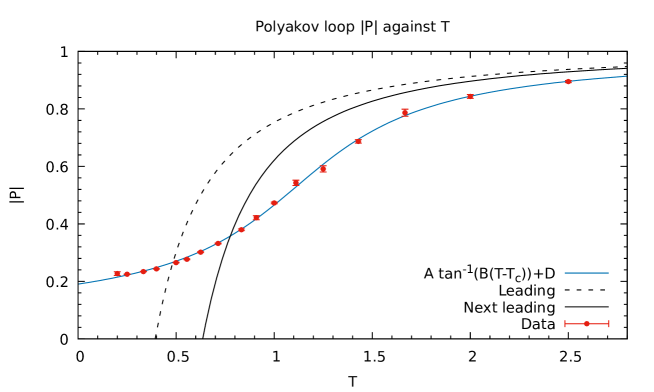
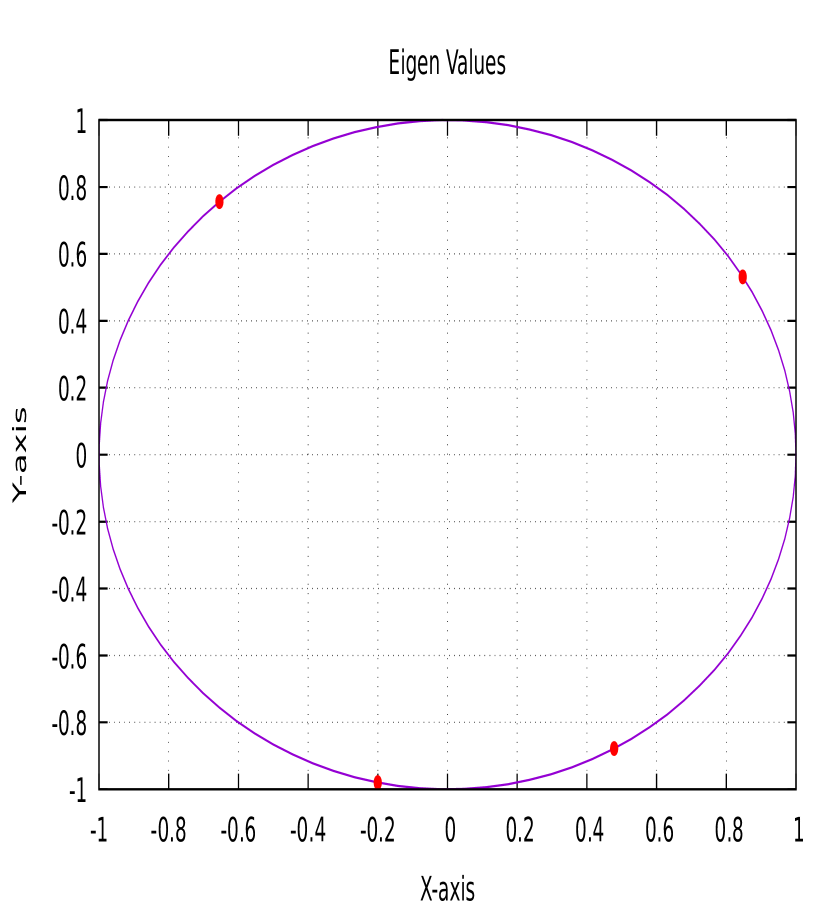
Refer to caption
Figure 4.2: Polyakov loop against temperature T𝑇T. The dotted and bold black curves show the leading order and the next-to-leading order terms of the high temperature expansion (HTE). The blue curve is the fitted curve to the plot. The phase transition occurs at Tc1.11subscript𝑇𝑐1.11T_{c}\approx 1.11.
Refer to caption
(a) Confined phase T=0.25𝑇0.25T=0.25.
Refer to caption
(b) Deconfined phase T=2.5𝑇2.5T=2.5.
Figure 4.3: Distribution of the eigenvalues of the Polyakov loop operator in the confined and deconfined phases.
Internal Energy E𝐸E and Extend of Space R2superscript𝑅2R^{2}

Fig. 4.4 shows the plot of the scaled internal energy EN2𝐸superscript𝑁2\frac{E}{N^{2}} against temperature T𝑇T. If we had simulated this for larger N𝑁N then we would clearly see a kink near the critical temperature, which would directly show that the system undergoes a phase transition. But for smaller N𝑁N this feature is not visible in the plot. The plot agrees well with the high temperature expansion (HTE). In Fig. 4.5 we show the plot of the extent of space R2superscript𝑅2R^{2} against temp T𝑇T.

Refer to caption
Figure 4.4: EN2𝐸superscript𝑁2\frac{E}{N^{2}} against temperature T𝑇T. The dotted and bold black curves show the leading order and the next-to-leading order terms of the high temperature expansion (HTE).
Refer to caption
Figure 4.5: Plot of R2superscript𝑅2R^{2} against temperature T𝑇T.

4.3 BFSS Matrix Model

The action of this model can be obtained by dimensionally reducing the 9+1919+1-dimensional 𝒩=1𝒩1\mathcal{N}=1 Super Yang-Mills theory to 0+1010+1 dimensions. The details of this model are given in Appendix A. The Euclidean action of the BFSS model is given by

SE=N2λ0β𝑑tTr{(DtXi)212[Xi,Xj]2+ψTC9DtψψTC9γi[Xi,ψ]},subscript𝑆𝐸𝑁2𝜆superscriptsubscript0𝛽differential-d𝑡tracesuperscriptsubscript𝐷𝑡superscript𝑋𝑖212superscriptsuperscript𝑋𝑖superscript𝑋𝑗2superscript𝜓𝑇subscript𝐶9subscript𝐷𝑡𝜓superscript𝜓𝑇subscript𝐶9superscript𝛾𝑖superscript𝑋𝑖𝜓\displaystyle S_{E}=\frac{N}{2\lambda}\int\limits_{0}^{\beta}dt\,\Tr\left\{(D_{t}X^{i})^{2}-\frac{1}{2}[X^{i},X^{j}]^{2}+\psi^{T}C_{9}D_{t}\psi-\psi^{T}C_{9}\gamma^{i}[X^{i},\psi]\right\}, (4.68)

where Dt=ti[A(t),]subscript𝐷𝑡subscript𝑡𝑖𝐴𝑡D_{t}=\partial_{t}-i[A(t),\cdot]; i,j=1,2,,9formulae-sequence𝑖𝑗129i,j=1,2,\cdots,9; Xisuperscript𝑋𝑖X^{i} are N×N𝑁𝑁N\times N traceless Hermitian matrices; λ𝜆\lambda is the ’t Hooft coupling; ψ𝜓\psi is a sixteen component Majorana fermion and each component of the fermion is an N×N𝑁𝑁N\times N traceless Hermitian matrix; C9subscript𝐶9C_{9} is the Euclidean charge conjugation matrix in the nine dimensions; and γisuperscript𝛾𝑖\gamma^{i} are the Euclidean gamma matrices in nine dimensions. Fermionic part of the action is obtained by taking a particular choice for the Majorana-Weyl fermion and the gamma matrices. The details are given in Ref. [Filev 16].

In this section we will simulate the quenched BFSS model, i.e., we will remove the fermions from the theory and we just simulate the bosonic part of this model. The Euclidean action of the bosonic part is given by

SE=N2λ0β𝑑tTr{(DtXi)212[Xi,Xj]2}.subscript𝑆𝐸𝑁2𝜆superscriptsubscript0𝛽differential-d𝑡tracesuperscriptsubscript𝐷𝑡superscript𝑋𝑖212superscriptsuperscript𝑋𝑖superscript𝑋𝑗2\displaystyle S_{E}=\frac{N}{2\lambda}\int\limits_{0}^{\beta}dt\,\Tr\left\{(D_{t}X^{i})^{2}-\frac{1}{2}[X^{i},X^{j}]^{2}\right\}. (4.69)

We see that the bosonic action is same as of the D=4𝐷4D=4 model but here we have nine scalar fields instead of three scalar fields. So the set of procedures from discretizing the action to applying the HMC remains the same. However, we discuss the important points below.

4.3.1 HMC for Bosonic BFSS Matrix Model

We introduce the momentum conjugate to Xnisubscriptsuperscript𝑋𝑖𝑛X^{i}_{n} to be Pnisubscriptsuperscript𝑃𝑖𝑛P^{i}_{n}, where Pnisubscriptsuperscript𝑃𝑖𝑛P^{i}_{n} is an N×N𝑁𝑁N\times N traceless Hermitian matrix and momentum conjugate to θksubscript𝜃𝑘\theta_{k} is Pksubscript𝑃𝑘P_{k}. The Hamiltonian for the molecular dynamics part of HMC is

H=n=0T112Tr(Pin2)+j=1N12Pj2+S[X,D(θ)]+SFP[θ].𝐻superscriptsubscript𝑛0𝑇112tracesuperscriptsuperscriptsubscript𝑃𝑖𝑛2superscriptsubscript𝑗1𝑁12superscriptsubscript𝑃𝑗2𝑆𝑋𝐷𝜃subscript𝑆𝐹𝑃delimited-[]𝜃\displaystyle H=\sum\limits_{n=0}^{T-1}\frac{1}{2}\Tr{{P_{i}^{n}}^{2}}+\sum\limits_{j=1}^{N}\frac{1}{2}P_{j}^{2}+S[X,D(\theta)]+S_{FP}[\theta]. (4.70)

The Hamilton’s equations are given by

X˙n,rsisuperscriptsubscript˙𝑋𝑛𝑟𝑠𝑖\displaystyle\dot{X}_{n,rs}^{i} =\displaystyle= HPn,sri=Pn,rsi,P˙n,rsi=HXn,sri,formulae-sequence𝐻superscriptsubscript𝑃𝑛𝑠𝑟𝑖superscriptsubscript𝑃𝑛𝑟𝑠𝑖superscriptsubscript˙𝑃𝑛𝑟𝑠𝑖𝐻superscriptsubscript𝑋𝑛𝑠𝑟𝑖\displaystyle\frac{\partial H}{\partial P_{n,sr}^{i}}=P_{n,rs}^{i},\qquad{\dot{P}_{n,rs}^{i}}=-\frac{\partial H}{\partial X_{n,sr}^{i}}, (4.71)
θ˙jsubscript˙𝜃𝑗\displaystyle\dot{\theta}_{j} =\displaystyle= HPj=Pj,P˙j=Hθj,formulae-sequence𝐻subscript𝑃𝑗subscript𝑃𝑗subscript˙𝑃𝑗𝐻subscript𝜃𝑗\displaystyle\frac{\partial H}{\partial P_{j}}=P_{j},\qquad\dot{P}_{j}=-\frac{\partial H}{\partial\theta_{j}}, (4.72)

where the dot represents time derivative with respect to the fictitious time τ𝜏\tau.

The forces can be calculated using the Hamiltonian, Eq. (4.70), and are given by

HX0,sri𝐻superscriptsubscript𝑋0𝑠𝑟𝑖\displaystyle-\frac{\partial H}{\partial X_{0,sr}^{i}} =\displaystyle= Naλ(X1i2X0i+DXT1iD)rs+Naλ[X0j,[X0i,X0j]]rs,𝑁𝑎𝜆subscriptsuperscriptsubscript𝑋1𝑖2superscriptsubscript𝑋0𝑖superscript𝐷superscriptsubscript𝑋𝑇1𝑖𝐷𝑟𝑠𝑁𝑎𝜆subscriptsuperscriptsubscript𝑋0𝑗superscriptsubscript𝑋0𝑖superscriptsubscript𝑋0𝑗𝑟𝑠\displaystyle\frac{N}{a\lambda}\left(X_{1}^{i}-2X_{0}^{i}+D^{\dagger}X_{T-1}^{i}D\right)_{rs}+\frac{Na}{\lambda}[X_{0}^{j},[X_{0}^{i},X_{0}^{j}]]_{rs},
HXn,sri𝐻superscriptsubscript𝑋𝑛𝑠𝑟𝑖\displaystyle-\frac{\partial H}{\partial X_{n,sr}^{i}} =\displaystyle= Naλ(Xn+1i2Xni+Xn1i)rs+Naλ[Xnj,[Xni,Xnj]]rsforn=1,2,,T2,𝑁𝑎𝜆subscriptsuperscriptsubscript𝑋𝑛1𝑖2superscriptsubscript𝑋𝑛𝑖superscriptsubscript𝑋𝑛1𝑖𝑟𝑠𝑁𝑎𝜆subscriptsuperscriptsubscript𝑋𝑛𝑗superscriptsubscript𝑋𝑛𝑖superscriptsubscript𝑋𝑛𝑗𝑟𝑠for𝑛12𝑇2\displaystyle\frac{N}{a\lambda}\left(X_{n+1}^{i}-2X_{n}^{i}+X_{n-1}^{i}\right)_{rs}+\frac{Na}{\lambda}[X_{n}^{j},[X_{n}^{i},X_{n}^{j}]]_{rs}~{}~{}\textrm{for}~{}~{}n=1,2,\cdots,T-2,
HXT1,sri𝐻superscriptsubscript𝑋𝑇1𝑠𝑟𝑖\displaystyle-\frac{\partial H}{\partial X_{T-1,sr}^{i}} =\displaystyle= Naλ(DX0iD2XT1i+XT2i)rs+Naλ[XT1j,[XT1i,XT1j]]rs,𝑁𝑎𝜆subscript𝐷superscriptsubscript𝑋0𝑖superscript𝐷2superscriptsubscript𝑋𝑇1𝑖superscriptsubscript𝑋𝑇2𝑖𝑟𝑠𝑁𝑎𝜆subscriptsuperscriptsubscript𝑋𝑇1𝑗superscriptsubscript𝑋𝑇1𝑖superscriptsubscript𝑋𝑇1𝑗𝑟𝑠\displaystyle\frac{N}{a\lambda}\left(DX_{0}^{i}D^{\dagger}-2X_{T-1}^{i}+X_{T-2}^{i}\right)_{rs}+\frac{Na}{\lambda}[X_{T-1}^{j},[X_{T-1}^{i},X_{T-1}^{j}]]_{rs},
Hθj𝐻subscript𝜃𝑗\displaystyle-\frac{\partial H}{\partial\theta_{j}} =\displaystyle= 2Naλk=1N𝔢(iXT1,kjiX0,jkiei(θjθk))+k=1kjNcot(θjθk2).2𝑁𝑎𝜆superscriptsubscript𝑘1𝑁𝔢𝑖subscriptsuperscript𝑋𝑖𝑇1𝑘𝑗subscriptsuperscript𝑋𝑖0𝑗𝑘superscript𝑒𝑖subscript𝜃𝑗subscript𝜃𝑘superscriptsubscript𝑘1𝑘𝑗𝑁subscript𝜃𝑗subscript𝜃𝑘2\displaystyle\frac{2N}{a\lambda}\sum\limits_{k=1}^{N}\mathfrak{Re}\left(iX^{i}_{T-1,kj}X^{i}_{0,jk}e^{i(\theta_{j}-\theta_{k})}\right)+\sum\limits_{\begin{subarray}{c}k=1\\ k\neq j\end{subarray}}^{N}\cot\left(\frac{\theta_{j}-\theta_{k}}{2}\right). (4.73)

Since DSU(N)𝐷𝑆𝑈𝑁D\in SU(N), all the θ𝜃\theta variables will not be independent and is constrained by the equation

i=1Nθi=0superscriptsubscript𝑖1𝑁subscript𝜃𝑖0\sum\limits_{i=1}^{N}\theta_{i}=0

as det(D)=1𝐷1\det(D)=1.

4.3.2 Observables

The observables we are interested in the bosonic BFSS model are the Polyakov loop |P|𝑃|P|, the extent of space R2superscript𝑅2R^{2} and the internal energy E𝐸E. The definitions and the discretized forms of the observables are given below

  • Polyakov loop |P|𝑃|P|

    |P|1N|P(ei𝑑tA(t))|=|Tr(D)N|(On lattice)formulae-sequencedelimited-⟨⟩𝑃1𝑁delimited-⟨⟩𝑃superscript𝑒𝑖contour-integraldifferential-d𝑡𝐴𝑡delimited-⟨⟩trace𝐷𝑁(On lattice)\displaystyle\left\langle|P|\right\rangle\equiv\frac{1}{N}\left\langle\left|P(e^{i\oint dtA(t)})\right|\right\rangle=\left\langle\left|\frac{\Tr(D)}{N}\right|\right\rangle~{}~{}~{}~{}\textrm{(On lattice)} (4.74)
  • Extent of space R2superscript𝑅2R^{2}

    R2λNβ0β𝑑tTr(Xi2)=λNTn=0T1Tr(Xni2)(Discretized form)formulae-sequencedelimited-⟨⟩superscript𝑅2delimited-⟨⟩𝜆𝑁𝛽superscriptsubscript0𝛽differential-d𝑡tracesuperscriptsuperscript𝑋𝑖2delimited-⟨⟩𝜆𝑁𝑇superscriptsubscript𝑛0𝑇1tracesuperscriptsubscriptsuperscript𝑋𝑖𝑛2(Discretized form)\displaystyle\left\langle R^{2}\right\rangle\equiv\left\langle\frac{\lambda}{N\beta}\int\limits_{0}^{\beta}dt\,\Tr({X^{i}}^{2})\right\rangle=\left\langle\frac{\lambda}{NT}\sum\limits_{n=0}^{T-1}\Tr({X^{i}_{n}}^{2})\right\rangle~{}~{}~{}~{}\textrm{(Discretized form)} (4.75)
  • Internal energy E𝐸E

    EN2delimited-⟨⟩𝐸superscript𝑁2\displaystyle\left\langle\frac{E}{N^{2}}\right\rangle \displaystyle\equiv 3λ4Nβ0β𝑑tTr([Xi,Xj]2)delimited-⟨⟩3𝜆4𝑁𝛽superscriptsubscript0𝛽differential-d𝑡tracesuperscriptsuperscript𝑋𝑖superscript𝑋𝑗2\displaystyle\left\langle-\frac{3\lambda}{4N\beta}\int\limits_{0}^{\beta}dt\,\Tr([X^{i},X^{j}]^{2})\right\rangle (4.76)
    =\displaystyle= 3λ4NTn=0T1Tr([Xni,Xnj]2)(Discretized form)delimited-⟨⟩3𝜆4𝑁𝑇superscriptsubscript𝑛0𝑇1tracesuperscriptsubscriptsuperscript𝑋𝑖𝑛subscriptsuperscript𝑋𝑗𝑛2(Discretized form)\displaystyle\left\langle-\frac{3\lambda}{4NT}\sum\limits_{n=0}^{T-1}\Tr([X^{i}_{n},X^{j}_{n}]^{2})\right\rangle~{}~{}~{}~{}\textrm{(Discretized form)}

4.3.3 Simulation Details

In simulations each variable and parameter has been measured in the unit of the ’t Hooft coupling λ0subscript𝜆0\lambda_{0}. Since the Yang-Mills coupling gYM2superscriptsubscript𝑔YM2g_{\rm YM}^{2} has a dimension of [L3superscript𝐿3L^{-3}] in one dimension, we can measure Xnisubscriptsuperscript𝑋𝑖𝑛X^{i}_{n} and A(n)𝐴𝑛A(n) in the unit of λ01/3superscriptsubscript𝜆013\lambda_{0}^{1/3}, and a𝑎a can be measured in units of λ01/3superscriptsubscript𝜆013\lambda_{0}^{-1/3}. Thus, each variable and parameter appearing in Eq. (4.53) is dimensionless. The values of the parameters used for this simulations are: N=4𝑁4N=4, T=10𝑇10T=10, d=9𝑑9d=9 and λ=1𝜆1\lambda=1. All the other details of the simulations are the same as the D=4𝐷4D=4 model. (See Sec. 4.2.3 for those details.)

We performed the simulations for 31 different temperature values each running for 800K Monte Carlo sweeps. The critical temperature Tcsubscript𝑇𝑐T_{c} comes out to be 0.9054(20)0.9054200.9054(20). Our results are in excellent agreement with those given in Refs. [Kawahara 07b] and [Filev 16].

Polyakov Loop |P|𝑃|P|

Fig. 4.6 shows the plot of the Polyakov loop |P|𝑃|P| against temperature T𝑇T. The values of the parameters for the fitted curve are given in Table 4.2. From this we conclude that the critical temperature Tc=0.9054(20)subscript𝑇𝑐0.905420T_{c}=0.9054(20).

Parameter Fit Value
A𝐴A 0.273982(1569)
B𝐵B 5.37305(8625)
Tcsubscript𝑇𝑐T_{c} 0.905404(2010)
D𝐷D 0.560378(1439)
Table 4.2: Values of the fitting parameters A𝐴A, B𝐵B, Tcsubscript𝑇𝑐T_{c} and D𝐷D.
Refer to caption
Figure 4.6: The Polyakov loop against temperature T𝑇T. The dotted and the bold black curves show the leading and the next-to-leading terms of the high temperature expansion (HTE) given in Ref. [Kawahara 07a]. The blue curve is the fitted curve to the data. The phase transition occurs at Tc0.905subscript𝑇𝑐0.905T_{c}\approx 0.905.
Internal Energy E𝐸E and Extent of Space R2superscript𝑅2R^{2}

In Fig. 4.7 we show the plot of the normalized internal energy EN2𝐸superscript𝑁2\frac{E}{N^{2}} against temperature T𝑇T. Our plot shows a smooth transition of EN2𝐸superscript𝑁2\frac{E}{N^{2}} across different phases but there should be a kink at Tcsubscript𝑇𝑐T_{c}. This kink becomes visible for larger N𝑁N, which is a clear indication of a second-order phase transition. In Ref. [Filev 16], the authors simulated the same model for N=16𝑁16N=16 and there we can clearly see a kink in the EN2𝐸superscript𝑁2\frac{E}{N^{2}} plot at Tcsubscript𝑇𝑐T_{c}. In Fig. 4.8 we show the plot of the extent of space R2superscript𝑅2R^{2} against temperature T𝑇T. We can see that all our plots are in excellent agreement with the high temperature expansion (HTE) predictions.
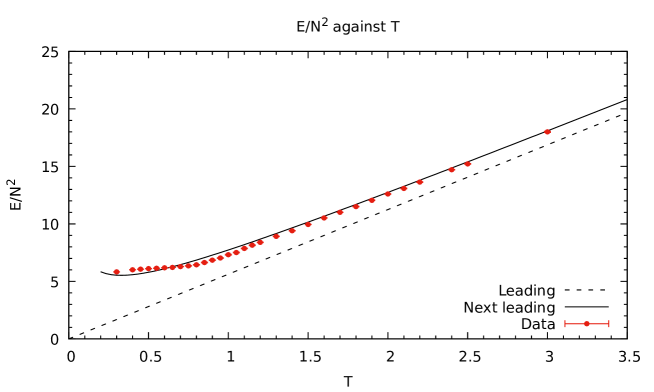
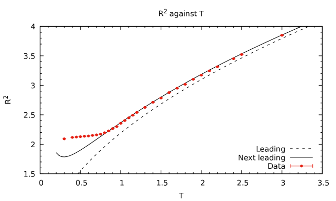
Refer to caption
Figure 4.7: The plot of EN2𝐸superscript𝑁2\frac{E}{N^{2}} against temperature T𝑇T. The dotted and bold black curves show the leading and the next-to-leading order terms of the high temperature expansion (HTE).
Refer to caption
Figure 4.8: The plot of extent of space R2superscript𝑅2R^{2} against temperature T𝑇T. The dotted and bold black curves show the leading and the next-to-leading order terms of the high temperature expansion (HTE).

Chapter 5 IKKT Matrix Model

In this chapter we discuss the numerical simulations of the bosonic IKKT Model. We also discuss the simulations of the model after the inclusion of fermions. We also discuss the simulations of the full IKKT Model.

5.1 Bosonic IKKT Matrix Model

This model is obtained by dimensionally reducing the Euclidean Yang-Mills action with gauge group SU(N)𝑆𝑈𝑁SU(N) from 9+1919+1 dimensions to 0+0000+0 dimensions. The Euclidean action of the model is given by

SE=14g2Tr([Xi,Xj]2),subscript𝑆E14superscript𝑔2tracesuperscriptsuperscript𝑋𝑖superscript𝑋𝑗2\displaystyle S_{\rm E}=-\frac{1}{4g^{2}}\Tr([X^{i},X^{j}]^{2}), (5.1)

where Xisuperscript𝑋𝑖X^{i} are N×N𝑁𝑁N\times N traceless Hermitian matrices, i,j𝑖𝑗i,j varies from 1,2,,1012101,2,\cdots,10 and g𝑔g is the Yang-Mills coupling in 0+0000+0 dimensions. We can replace g𝑔g with λ𝜆\lambda the ’t Hooft coupling, which follows the relation λ=Ng2𝜆𝑁superscript𝑔2\lambda=Ng^{2}. The action then takes the form

SE=N4λTr([Xi,Xj]2).subscript𝑆E𝑁4𝜆tracesuperscriptsuperscript𝑋𝑖superscript𝑋𝑗2\displaystyle S_{\rm E}=-\frac{N}{4\lambda}\Tr([X^{i},X^{j}]^{2}). (5.2)

Now by rescaling the fields we can absorb λ𝜆\lambda into the field variables. If we rescale the fields by Xiλ1/4Xisuperscript𝑋𝑖superscript𝜆14superscript𝑋𝑖X^{i}\rightarrow\lambda^{1/4}X^{i}, then λ𝜆\lambda will be absorbed in the field variables and the action simplifies to

SE=N4Tr([Xi,Xj]2).subscript𝑆E𝑁4tracesuperscriptsuperscript𝑋𝑖superscript𝑋𝑗2\displaystyle S_{\rm E}=-\frac{N}{4}\Tr([X^{i},X^{j}]^{2}). (5.3)

In the above action all the field variables are dimensionless. The action is gauge invariant under the following gauge transformation

XiVXiV,superscript𝑋𝑖𝑉superscript𝑋𝑖superscript𝑉\displaystyle X^{i}\longrightarrow VX^{i}V^{\dagger}, (5.4)

where VSU(N)𝑉𝑆𝑈𝑁V\in SU(N). The partition function of this model is given by

Z=𝒟Xexp(SE).𝑍𝒟𝑋subscript𝑆E\displaystyle Z=\int\mathcal{D}X\,\,\exp{-S_{\rm E}}. (5.5)

Apart from this gauge symmetry, the action Eq. (5.3) also has SO(10)𝑆𝑂10SO(10) symmetry. That is, if we change Xisuperscript𝑋𝑖X^{i} by the transformation

XiOikXk,superscript𝑋𝑖subscript𝑂𝑖𝑘superscript𝑋𝑘\displaystyle X^{i}\longrightarrow O_{ik}X^{k}, (5.6)

where OSO(10)𝑂𝑆𝑂10O\in SO(10), the action remains invariant. Changing the fields with this transformation, the action becomes

SEsubscript𝑆E\displaystyle S_{\rm E} =N4Tr([OikXk,OjlXl][OimXm,OjnXn])absent𝑁4tracesubscript𝑂𝑖𝑘superscript𝑋𝑘subscript𝑂𝑗𝑙superscript𝑋𝑙subscript𝑂𝑖𝑚superscript𝑋𝑚subscript𝑂𝑗𝑛superscript𝑋𝑛\displaystyle=-\frac{N}{4}\Tr([O_{ik}X^{k},O_{jl}X^{l}][O_{im}X^{m},O_{jn}X^{n}])
=N4OikOimOjlOjnTr([Xk,Xl][Xm,Xn])absent𝑁4subscript𝑂𝑖𝑘subscript𝑂𝑖𝑚subscript𝑂𝑗𝑙subscript𝑂𝑗𝑛tracesuperscript𝑋𝑘superscript𝑋𝑙superscript𝑋𝑚superscript𝑋𝑛\displaystyle=-\frac{N}{4}O_{ik}O_{im}O_{jl}O_{jn}\Tr([X^{k},X^{l}][X^{m},X^{n}])
=N4δkmδlnTr([Xk,Xl][Xm,Xn]) using OikOim=δkmformulae-sequenceabsent𝑁4subscript𝛿𝑘𝑚subscript𝛿𝑙𝑛tracesuperscript𝑋𝑘superscript𝑋𝑙superscript𝑋𝑚superscript𝑋𝑛 using subscript𝑂𝑖𝑘subscript𝑂𝑖𝑚subscript𝛿𝑘𝑚\displaystyle=-\frac{N}{4}\delta_{km}\delta_{ln}\Tr([X^{k},X^{l}][X^{m},X^{n}])\qquad\textrm{ using }O_{ik}O_{im}=\delta_{km}
=N4Tr([Xk,Xl]2).absent𝑁4tracesuperscriptsuperscript𝑋𝑘superscript𝑋𝑙2\displaystyle=-\frac{N}{4}\Tr([X^{k},X^{l}]^{2}). (5.7)

Thus the action remains invariant under this transformation telling us that SO(10)𝑆𝑂10SO(10) is a symmetry of this system. Putting this theory on the lattice is a trivial task as this model is 00-dimensional, and thus everything is happening on a single lattice site. The action Eq. (5.3) itself represents the action of the continuum theory as well as of the lattice theory.

5.1.1 HMC for Bosonic IKKT Matrix Model

We will now introduce conjugate momenta for each of the field variable. The momenta conjugate to Xisuperscript𝑋𝑖X^{i} is Pisuperscript𝑃𝑖P^{i}, where Pisuperscript𝑃𝑖P^{i} is an N×N𝑁𝑁N\times N traceless Hermitian matrix. The Hamiltonian for the molecular dynamics part of the HMC is given by

H=12i=110Tr(Pi2)N4i,j=110Tr([Xi,Xj]2).𝐻12superscriptsubscript𝑖110tracesuperscriptsuperscript𝑃𝑖2𝑁4superscriptsubscript𝑖𝑗110tracesuperscriptsuperscript𝑋𝑖superscript𝑋𝑗2\displaystyle H=\frac{1}{2}\sum\limits_{i=1}^{10}\Tr({P^{i}}^{2})-\frac{N}{4}\sum\limits_{i,j=1}^{10}\Tr([X^{i},X^{j}]^{2}). (5.8)

Hamilton’s equations are given by

X˙rsi=HPsri=Prsi,P˙rsi=HXsri,formulae-sequencesuperscriptsubscript˙𝑋𝑟𝑠𝑖𝐻superscriptsubscript𝑃𝑠𝑟𝑖superscriptsubscript𝑃𝑟𝑠𝑖superscriptsubscript˙𝑃𝑟𝑠𝑖𝐻superscriptsubscript𝑋𝑠𝑟𝑖\displaystyle\dot{X}_{rs}^{i}=\frac{\partial H}{\partial P_{sr}^{i}}=P_{rs}^{i},\qquad{\dot{P}_{rs}^{i}}=-\frac{\partial H}{\partial X_{sr}^{i}}, (5.9)

where the dot represents time derivative with respect to the fictitious time τ𝜏\tau.

The forces can be calculated using the Hamiltonian, Eq. (5.8), and are given by

HXsri=Nj=1ji10[Xj,[Xi,Xj]]rs.𝐻superscriptsubscript𝑋𝑠𝑟𝑖𝑁superscriptsubscript𝑗1𝑗𝑖10subscriptsuperscript𝑋𝑗superscript𝑋𝑖superscript𝑋𝑗𝑟𝑠\displaystyle-\frac{\partial H}{\partial X_{sr}^{i}}=N\sum\limits_{\begin{subarray}{c}j=1\\ j\neq i\end{subarray}}^{10}[X^{j},[X^{i},X^{j}]]_{rs}. (5.10)

5.1.2 Observables

The observables we are interested in the IKKT model are the extent of spacetime R2superscript𝑅2R^{2} and eigenvalues of the moment of inertia tensor Iμνsubscript𝐼𝜇𝜈I_{\mu\nu}. The definitions of the observables are given below

  • Extent of spacetime R2superscript𝑅2R^{2}

    R2=1NTr(Xi2).delimited-⟨⟩superscript𝑅2delimited-⟨⟩1𝑁tracesuperscriptsuperscript𝑋𝑖2\displaystyle\left\langle R^{2}\right\rangle=\left\langle\frac{1}{N}\Tr({X^{i}}^{2})\right\rangle. (5.11)
  • Eigenvalues of moment of inertia tensor Iμνsubscript𝐼𝜇𝜈I_{\mu\nu}

    Iμν=1NTr(XμXν).subscript𝐼𝜇𝜈1𝑁tracesuperscript𝑋𝜇superscript𝑋𝜈\displaystyle I_{\mu\nu}=\frac{1}{N}\Tr(X^{\mu}X^{\nu}). (5.12)

Eigenvalues of the moment of inertia tensor are λisubscript𝜆𝑖\lambda_{i}, i=1,2,,10𝑖1210i=1,2,\cdots,10.

5.1.3 Simulation Details and Results

We simulated this model for different values of N𝑁N. Simulating this model is quite easy compared to the BFSS model. Again to save time, we run the simulation for each N𝑁N on a single core of the computer. This way, we were able to run the simulations for all the values of N𝑁N simultaneously using multiple cores at the same time. Here we can see that the simulation depends on N𝑁N itself, so it will take different time for each N𝑁N.

We performed the simulations for 10 different values of N𝑁N each running for 110K Monte Carlo sweeps. The results are provided below. Basically, our aim is to study how the system behaves at large N𝑁N.

Eigenvalues of Iμνsubscript𝐼𝜇𝜈I_{\mu\nu}

Figure 5.1 shows the plot of the eigenvalues of Iμνsubscript𝐼𝜇𝜈I_{\mu\nu} against 1N1𝑁\frac{1}{N}. We can see in the plot that the eigenvalues are converging towards a single point. This shows that we do not encounter SO(10)𝑆𝑂10SO(10) spontaneous symmetry breaking (SSB) in the limit N𝑁N\rightarrow\infty. This same conclusion was also drawn in the Ref. [Hotta 99]. However, they used different criteria to arrive at this conclusion.
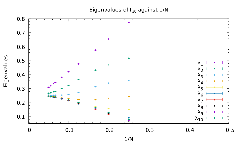
Refer to caption
Figure 5.1: Plot of the eigenvalues of Iμνsubscript𝐼𝜇𝜈I_{\mu\nu} against 1N1𝑁\frac{1}{N}. We can see that the eigenvalues are converging towards a single point for large N𝑁N.
Extent of spacetime R2superscript𝑅2R^{2}

In Fig. 5.2 we show the plot of the extent of spacetime R2superscript𝑅2R^{2} against 1N1𝑁\frac{1}{N}.

Refer to caption
Figure 5.2: Extent of spacetime R2superscript𝑅2R^{2} against 1N1𝑁\frac{1}{N}.

We can also arrive at the same conclusion using the extent of spacetime. But here we calculate Ri2=1NTr(Xi2)superscriptsubscript𝑅𝑖21𝑁tracesuperscriptsuperscript𝑋𝑖2R_{i}^{2}=\frac{1}{N}\Tr({X^{i}}^{2}) and this time we do not have a sum over repeated indices. If we plot these Risubscript𝑅𝑖R_{i}’s, then we will see that all of them converges to the same value in the limit N𝑁N\rightarrow\infty. This will also indicate that there is no SSB of SO(10)𝑆𝑂10SO(10) in the limit N𝑁N\rightarrow\infty. If there is SSB of SO(10)𝑆𝑂10SO(10), then some d𝑑d values of Risubscript𝑅𝑖R_{i} will have smaller values as compared to the remaining ones in the limit N𝑁N\rightarrow\infty. This way we will conclude that the SO(10)𝑆𝑂10SO(10) will spontaneously break to SO(d)×SO(10d)𝑆𝑂𝑑𝑆𝑂10𝑑SO(d)\times SO(10-d).

5.2 Full IKKT Matrix Model

We will now add fermions in our theory and study the full IKKT matrix model. This model is obtained by dimensionally reducing the 𝒩=1𝒩1\mathcal{N}=1 super Yang-Mills model in 9+1919+1 dimensions to 0+0000+0 dimensions or dimensionally reducing the BFSS model to 0+0000+0 dimensions. The Euclidean action is given by

SE=N4λTr([Xi,Xj]2)N2λψα(C9γi)αβ[Xi,ψβ],subscript𝑆E𝑁4𝜆tracesuperscriptsuperscript𝑋𝑖superscript𝑋𝑗2𝑁2𝜆subscript𝜓𝛼subscriptsubscript𝐶9superscript𝛾𝑖𝛼𝛽superscript𝑋𝑖subscript𝜓𝛽\displaystyle S_{\rm E}=-\frac{N}{4\lambda}\Tr([X^{i},X^{j}]^{2})-\frac{N}{2\lambda}\psi_{\alpha}(C_{9}\gamma^{i})_{\alpha\beta}[X^{i},\psi_{\beta}], (5.13)

where i,j=1,2,,10formulae-sequence𝑖𝑗1210i,j=1,2,\cdots,10; α,β=1,2,,16formulae-sequence𝛼𝛽1216\alpha,\beta=1,2,\cdots,16; Xisuperscript𝑋𝑖X^{i} are N×N𝑁𝑁N\times N traceless Hermitian matrices; λ𝜆\lambda is the ’t Hooft coupling; ψ𝜓\psi is a sixteen component Majorana fermion with each component of the fermion being an N×N𝑁𝑁N\times N traceless Hermitian matrix; C9subscript𝐶9C_{9} is the Euclidean charge conjugation matrix in the nine dimensions; and γisuperscript𝛾𝑖\gamma^{i} are the Euclidean gamma matrices in nine dimensions. Fermionic part of the action is obtained by taking a particular choice for the Majorana-Weyl fermion. The details are given in Ref. [Filev 16]. The choice of gamma matrices are such that the charge conjugation matrix becomes identity matrix in this representation. The details of the choice of gamma matrices are given in the Ref. [Ambjørn 00]. In this representation of gamma matrices the action simplifies to

SE=N4λTr([Xi,Xj]2)N2λTr(ψαγαβi[Xi,ψβ]).subscript𝑆E𝑁4𝜆tracesuperscriptsuperscript𝑋𝑖superscript𝑋𝑗2𝑁2𝜆tracesubscript𝜓𝛼subscriptsuperscript𝛾𝑖𝛼𝛽superscript𝑋𝑖subscript𝜓𝛽\displaystyle S_{\rm E}=-\frac{N}{4\lambda}\Tr([X^{i},X^{j}]^{2})-\frac{N}{2\lambda}\Tr(\psi_{\alpha}\gamma^{i}_{\alpha\beta}[X^{i},\psi_{\beta}]). (5.14)

The action is invariant under the following gauge transformation

Xisuperscript𝑋𝑖absent\displaystyle X^{i}\longrightarrow VXiV,𝑉superscript𝑋𝑖superscript𝑉\displaystyle VX^{i}V^{\dagger},
ψαsubscript𝜓𝛼absent\displaystyle\psi_{\alpha}\longrightarrow VψαV,𝑉subscript𝜓𝛼superscript𝑉\displaystyle V\psi_{\alpha}V^{\dagger}, (5.15)

where VSU(N)𝑉𝑆𝑈𝑁V\in SU(N). Apart from the gauge symmetry, the action also remains invariant under SO(10)𝑆𝑂10SO(10) symmetry as Xisuperscript𝑋𝑖X^{i} transforms as a vector and ψ𝜓\psi transforms as a Majorana-Weyl spinor under this transformation. The partition function of this model is given by

Z=𝒟X𝒟ψexp(SE).𝑍𝒟𝑋𝒟𝜓subscript𝑆E\displaystyle Z=\int\mathcal{D}X\,\,\mathcal{D}\psi\,\,\exp{-S_{\rm E}}. (5.16)

We can integrate out the fermions from this partition function. For that, we first need to form the fermion matrix. We can simplify the fermionic part of the action to get the fermion matrix. First, we will decompose the fields with the help of the SU(N)𝑆𝑈𝑁SU(N) generators.

Xi=superscript𝑋𝑖absent\displaystyle X^{i}= XaiTa,subscriptsuperscript𝑋𝑖𝑎subscript𝑇𝑎\displaystyle X^{i}_{a}T_{a},
ψα=subscript𝜓𝛼absent\displaystyle\psi_{\alpha}= ψαaTa.superscriptsubscript𝜓𝛼𝑎subscript𝑇𝑎\displaystyle\psi_{\alpha}^{a}T_{a}. (5.17)

Substituting this in the fermionic part of the action, we get

Sf=subscript𝑆fabsent\displaystyle S_{\rm f}= N2λTr(ψαaTaγαβj[XbjTb,ψβcTc])𝑁2𝜆tracesuperscriptsubscript𝜓𝛼𝑎subscript𝑇𝑎subscriptsuperscript𝛾𝑗𝛼𝛽subscriptsuperscript𝑋𝑗𝑏subscript𝑇𝑏superscriptsubscript𝜓𝛽𝑐subscript𝑇𝑐\displaystyle-\frac{N}{2\lambda}\Tr(\psi_{\alpha}^{a}T_{a}\gamma^{j}_{\alpha\beta}[X^{j}_{b}T_{b},\psi_{\beta}^{c}T_{c}])
=\displaystyle= N2λψαaγαβjXbjψβcTr(Ta[Tb,Tc])𝑁2𝜆superscriptsubscript𝜓𝛼𝑎subscriptsuperscript𝛾𝑗𝛼𝛽subscriptsuperscript𝑋𝑗𝑏superscriptsubscript𝜓𝛽𝑐tracesubscript𝑇𝑎subscript𝑇𝑏subscript𝑇𝑐\displaystyle-\frac{N}{2\lambda}\psi_{\alpha}^{a}\gamma^{j}_{\alpha\beta}X^{j}_{b}\psi_{\beta}^{c}\Tr(T_{a}[T_{b},T_{c}])
=\displaystyle= N2λψαaγαβjXbjψβc(ifbcd)Tr(TaTd) using [Tb,Tc]=ifbcdTd𝑁2𝜆superscriptsubscript𝜓𝛼𝑎subscriptsuperscript𝛾𝑗𝛼𝛽subscriptsuperscript𝑋𝑗𝑏superscriptsubscript𝜓𝛽𝑐𝑖subscript𝑓𝑏𝑐𝑑tracesubscript𝑇𝑎subscript𝑇𝑑 using subscript𝑇𝑏subscript𝑇𝑐𝑖subscript𝑓𝑏𝑐𝑑subscript𝑇𝑑\displaystyle-\frac{N}{2\lambda}\psi_{\alpha}^{a}\gamma^{j}_{\alpha\beta}X^{j}_{b}\psi_{\beta}^{c}(if_{bcd})\Tr(T_{a}T_{d})\qquad\textrm{ using }[T_{b},T_{c}]=if_{bcd}T_{d}
=\displaystyle= iN2λψαaγαβjXbjψβcfbca using Tr(TaTb)=δab𝑖𝑁2𝜆superscriptsubscript𝜓𝛼𝑎subscriptsuperscript𝛾𝑗𝛼𝛽subscriptsuperscript𝑋𝑗𝑏superscriptsubscript𝜓𝛽𝑐subscript𝑓𝑏𝑐𝑎 using tracesubscript𝑇𝑎subscript𝑇𝑏subscript𝛿𝑎𝑏\displaystyle\,\,\frac{iN}{2\lambda}\psi_{\alpha}^{a}\gamma^{j}_{\alpha\beta}X^{j}_{b}\psi_{\beta}^{c}f_{bca}\qquad\textrm{ using }\Tr(T_{a}T_{b})=-\delta_{ab}
=\displaystyle= ψαa(iN2λγαβjXcjfabc)ψβb using totally antisymmetric property of fabcsuperscriptsubscript𝜓𝛼𝑎𝑖𝑁2𝜆subscriptsuperscript𝛾𝑗𝛼𝛽subscriptsuperscript𝑋𝑗𝑐subscript𝑓𝑎𝑏𝑐superscriptsubscript𝜓𝛽𝑏 using totally antisymmetric property of subscript𝑓𝑎𝑏𝑐\displaystyle\,\,\psi_{\alpha}^{a}\left(-\frac{iN}{2\lambda}\gamma^{j}_{\alpha\beta}X^{j}_{c}f_{abc}\right)\psi_{\beta}^{b}\qquad\textrm{ using totally antisymmetric property of }f_{abc}
=\displaystyle= ψαaαa,βbψβb,superscriptsubscript𝜓𝛼𝑎subscript𝛼𝑎𝛽𝑏superscriptsubscript𝜓𝛽𝑏\displaystyle\,\,\psi_{\alpha}^{a}\,\,\mathcal{M}_{\alpha a,\beta b}\,\,\psi_{\beta}^{b}, (5.18)

where

αa,βb=iN2λγαβjXcjfabc=N2λγαβjTr(Xj[Ta,Tb]),subscript𝛼𝑎𝛽𝑏𝑖𝑁2𝜆subscriptsuperscript𝛾𝑗𝛼𝛽subscriptsuperscript𝑋𝑗𝑐subscript𝑓𝑎𝑏𝑐𝑁2𝜆subscriptsuperscript𝛾𝑗𝛼𝛽tracesuperscript𝑋𝑗subscript𝑇𝑎subscript𝑇𝑏\displaystyle\mathcal{M}_{\alpha a,\beta b}=-\frac{iN}{2\lambda}\gamma^{j}_{\alpha\beta}X^{j}_{c}f_{abc}=\frac{N}{2\lambda}\gamma^{j}_{\alpha\beta}\Tr(X^{j}[T_{a},T_{b}]), (5.19)

with a,b,c=1,2,,N21formulae-sequence𝑎𝑏𝑐12superscript𝑁21a,b,c=1,2,\cdots,N^{2}-1 and α,β=1,2,,16formulae-sequence𝛼𝛽1216\alpha,\beta=1,2,\cdots,16. The fermion matrix αa,βbsubscript𝛼𝑎𝛽𝑏\mathcal{M}_{\alpha a,\beta b} is a 16(N21)×16(N21)16superscript𝑁2116superscript𝑁2116(N^{2}-1)\times 16(N^{2}-1) size matrix. Now using the result that

𝑑ψexp(ψTAψ)=Pf(A)=det(A)1/2where A is an antisymmetric matrixformulae-sequencedifferential-d𝜓superscript𝜓𝑇𝐴𝜓Pf𝐴superscript𝐴12where 𝐴 is an antisymmetric matrix\displaystyle\int d\psi\,\,\exp{-\psi^{T}A\psi}=\textrm{Pf}(A)=\det(A)^{1/2}\qquad\textrm{where }A\textrm{ is an antisymmetric matrix} (5.20)

we can integrate out the fermions from the partition function Eq. (5.16). Integrating out the fermions from the partition function we get

Z=𝒟Xexp(Sb)Pf(),𝑍𝒟𝑋subscript𝑆bPf\displaystyle Z=\int\mathcal{D}X\,\,\exp{-S_{\rm b}}\,\,\textrm{Pf}(\mathcal{M}), (5.21)

where Sbsubscript𝑆bS_{\rm b} is the bosonic part of the action. Pf()Pf\textrm{Pf}(\mathcal{M}) for this model comes to be a complex number. Since Pf()Pf\textrm{Pf}(\mathcal{M}) is a complex number so we cannot treat exp(SE)subscript𝑆E\exp{-S_{\rm E}} as the probability distribution. This is known as the sign problem. There are methods to deal with this problem by using other techniques like Lefschetz thimbles and complex Langevin with stochastic quantization.

One another technique is to consider only the absolute part of the Pfaffian in the partition function and monitor the phase of the Pfaffian during the simulations. If the phase of the Pfaffian does not vary much, then the Monte Carlo simulations can be trusted, but if it varies too much than we cannot trust the Monte Carlo simulations. We are going to use this technique for our simulation. So our partition function becomes

Z=𝒟Xexp(Sb)|Pf()|.𝑍𝒟𝑋subscript𝑆bPf\displaystyle Z=\int\mathcal{D}X\,\,\exp{-S_{\rm b}}\,\,\left|\textrm{Pf}(\mathcal{M})\right|. (5.22)

For calculation of Pf()=det()1/2Pfsuperscript12\textrm{Pf}(\mathcal{M})=\det(\mathcal{M})^{1/2} our best algorithm provides the time complexity of 𝒪(N6)𝒪superscript𝑁6\mathcal{O}(N^{6}). So calculating this determinant is quite a computationally heavy task. So we do not calculate this determinant directly, rather we use a rational approximation to approximate this determinant within certain error for our simulation purpose. The details are provided in the next section.

5.2.1 RHMC and Fermionic Forces

We can write the absolute value of the Pfaffian as

|Pf()|=det()1/4,Pfsuperscriptsuperscript14\displaystyle\left|\textrm{Pf}(\mathcal{M})\right|=\det(\mathcal{M}^{\dagger}\,\mathcal{M})^{1/4}, (5.23)

and using the result

𝑑ψ𝑑ψexp(ψAψ)1det(A)where A=Aformulae-sequenceproportional-todifferential-d𝜓differential-dsuperscript𝜓superscript𝜓𝐴𝜓1𝐴where 𝐴superscript𝐴\displaystyle\int d\psi\,d\psi^{\dagger}\,\,\exp{-\psi^{\dagger}A\psi}\propto\frac{1}{\det(A)}\qquad\textrm{where }A=A^{\dagger} (5.24)

we can write

det()1/4𝑑ξ𝑑ξexp(ξ()1/4ξ).proportional-tosuperscriptsuperscript14differential-d𝜉differential-dsuperscript𝜉superscript𝜉superscriptsuperscript14𝜉\displaystyle\det(\mathcal{M}^{\dagger}\,\mathcal{M})^{1/4}\propto\int d\xi\,d\xi^{\dagger}\,\,\exp{-\xi^{\dagger}\,(\mathcal{M}^{\dagger}\,\mathcal{M})^{-1/4}\,\xi}. (5.25)

So the partition function becomes

Z𝒟X𝑑ξ𝑑ξexp(Sb[X]Spsf),proportional-to𝑍𝒟𝑋differential-d𝜉differential-dsuperscript𝜉subscript𝑆bdelimited-[]𝑋subscript𝑆psf\displaystyle Z\propto\int\mathcal{D}X\,d\xi\,d\xi^{\dagger}\,\,\exp{-S_{\rm b}[X]-S_{\rm psf}}, (5.26)

where

Spsf=ξ()1/4ξ,subscript𝑆psfsuperscript𝜉superscriptsuperscript14𝜉\displaystyle S_{\rm ps\,f}=\xi^{\dagger}\,(\mathcal{M}^{\dagger}\,\mathcal{M})^{-1/4}\,\xi, (5.27)

with ξ𝜉\xi being a 16(N21)16superscript𝑁2116(N^{2}-1)-dimensional complex vector known as the pseudo-fermion fields. Spsfsubscript𝑆psfS_{\rm ps\,f} is known as the pseudo-fermion action. First we note that if we define

η=()1/8ξ𝜂superscriptsuperscript18𝜉\displaystyle\eta=(\mathcal{M}^{\dagger}\,\mathcal{M})^{-1/8}\xi (5.28)

then the pseudo-fermion action becomes Spsf=ηηsubscript𝑆psfsuperscript𝜂𝜂S_{\rm ps\,f}=\eta^{\dagger}\,\eta. Then we can simply take η𝜂\eta randomly from the Gaussian distribution and using Eq. (5.28) we get the value of ξ𝜉\xi. But the main question is how to calculate ()1/8superscriptsuperscript18(\mathcal{M}^{\dagger}\,\mathcal{M})^{-1/8}. For this we use the rational approximation to approximate this and after that we can calculate ξ𝜉\xi. The idea is to approximate the rational exponent of the superscript\mathcal{M}^{\dagger}\,\mathcal{M} with the partial sum

()d=α0+i=1pαi(+βi 1)1,superscriptsuperscript𝑑subscript𝛼0superscriptsubscript𝑖1𝑝subscript𝛼𝑖superscriptsuperscriptsubscript𝛽𝑖11\displaystyle(\mathcal{M}^{\dagger}\,\mathcal{M})^{d}=\alpha_{0}+\sum\limits_{i=1}^{p}\alpha_{i}(\mathcal{M}^{\dagger}\,\mathcal{M}+\beta_{i}\,\mathbb{1})^{-1}, (5.29)

where d𝑑d is the rational exponent, which we require for our calculation purpose and p𝑝p depends on the accuracy of the approximation. If we want more accurate results then we will use a large value for p𝑝p. Remez algorithm is used to obtain α0,αisubscript𝛼0subscript𝛼𝑖\alpha_{0},\,\alpha_{i} and βisubscript𝛽𝑖\beta_{i}. The detailed theory of rational approximation is given in Ref. [Ydri 17] and the program of the Remez algorithm is on Github as an open source code - see Ref. [Clark 05]. To calculate ξ𝜉\xi we require d=1/8𝑑18d=1/8. Then, we use the rational approximation to calculate ξ𝜉\xi from η𝜂\eta. We call this algorithm the RHMC algorithm since the rational approximation is used to approximate ()dsuperscriptsuperscript𝑑(\mathcal{M}^{\dagger}\,\mathcal{M})^{d}, and HMC is used to generate the states distributed according to the probability distribution.

The momentum conjugate to Xisuperscript𝑋𝑖X^{i} is Pisuperscript𝑃𝑖P^{i}, where Pisuperscript𝑃𝑖P^{i} is an N×N𝑁𝑁N\times N traceless Hermitian matrix. We do not introduce momentum variable for pseudo-fermion fields as they are already distributed according to the required probability distribution. So the Hamiltonian of the system is given by

H=12Tr(Pi2)N4λTr([Xi,Xj]2)+ξ()1/4ξ.𝐻12tracesuperscriptsuperscript𝑃𝑖2𝑁4𝜆tracesuperscriptsuperscript𝑋𝑖superscript𝑋𝑗2superscript𝜉superscriptsuperscript14𝜉\displaystyle H=\frac{1}{2}\Tr({P^{i}}^{2})-\frac{N}{4\lambda}\Tr([X^{i},X^{j}]^{2})+\xi^{\dagger}\,(\mathcal{M}^{\dagger}\,\mathcal{M})^{-1/4}\,\xi. (5.30)

Thus we require two rational approximations, one for d=1/8𝑑18d=1/8 and other for d=1/4𝑑14d=-1/4. So

()1/8=α0+i=1pαi(+βi 1)1superscriptsuperscript18subscript𝛼0superscriptsubscript𝑖1𝑝subscript𝛼𝑖superscriptsuperscriptsubscript𝛽𝑖11\displaystyle(\mathcal{M}^{\dagger}\,\mathcal{M})^{1/8}=\alpha_{0}+\sum\limits_{i=1}^{p}\alpha_{i}(\mathcal{M}^{\dagger}\,\mathcal{M}+\beta_{i}\,\mathbb{1})^{-1} (5.31)
()1/4=a0+i=1qai(+bi 1)1.superscriptsuperscript14subscript𝑎0superscriptsubscript𝑖1𝑞subscript𝑎𝑖superscriptsuperscriptsubscript𝑏𝑖11\displaystyle(\mathcal{M}^{\dagger}\,\mathcal{M})^{-1/4}=a_{0}+\sum\limits_{i=1}^{q}a_{i}(\mathcal{M}^{\dagger}\,\mathcal{M}+b_{i}\,\mathbb{1})^{-1}. (5.32)

Substituting the value of ()1/4superscriptsuperscript14(\mathcal{M}^{\dagger}\,\mathcal{M})^{-1/4} back in Eq. (5.30) we get

H=12Tr(Pi2)N4λTr([Xi,Xj]2)+ξ(a0ξ+i=1qai(+bi 1)1ξ).𝐻12tracesuperscriptsuperscript𝑃𝑖2𝑁4𝜆tracesuperscriptsuperscript𝑋𝑖superscript𝑋𝑗2superscript𝜉subscript𝑎0𝜉superscriptsubscript𝑖1𝑞subscript𝑎𝑖superscriptsuperscriptsubscript𝑏𝑖11𝜉\displaystyle H=\frac{1}{2}\Tr({P^{i}}^{2})-\frac{N}{4\lambda}\Tr([X^{i},X^{j}]^{2})+\xi^{\dagger}\,\left(a_{0}\xi+\sum\limits_{i=1}^{q}a_{i}(\mathcal{M}^{\dagger}\,\mathcal{M}+b_{i}\,\mathbb{1})^{-1}\xi\right). (5.33)

Hamilton’s equations are given by

X˙rsi=HPsri=Prsi,P˙rsi=HXsriformulae-sequencesuperscriptsubscript˙𝑋𝑟𝑠𝑖𝐻superscriptsubscript𝑃𝑠𝑟𝑖superscriptsubscript𝑃𝑟𝑠𝑖superscriptsubscript˙𝑃𝑟𝑠𝑖𝐻superscriptsubscript𝑋𝑠𝑟𝑖\displaystyle\dot{X}_{rs}^{i}=\frac{\partial H}{\partial P_{sr}^{i}}=P_{rs}^{i},\qquad{\dot{P}_{rs}^{i}}=-\frac{\partial H}{\partial X_{sr}^{i}} (5.34)

where the dot represents time derivative with respect to the fictitious time τ𝜏\tau.

The forces can be calculated using the Hamiltonian, Eq. (5.33), and are given by

HXsri=Nj=1ji10[Xj,[Xi,Xj]]rsSpsfXsri,𝐻superscriptsubscript𝑋𝑠𝑟𝑖𝑁superscriptsubscript𝑗1𝑗𝑖10subscriptsuperscript𝑋𝑗superscript𝑋𝑖superscript𝑋𝑗𝑟𝑠subscript𝑆psfsuperscriptsubscript𝑋𝑠𝑟𝑖\displaystyle-\frac{\partial H}{\partial X_{sr}^{i}}=N\sum\limits_{\begin{subarray}{c}j=1\\ j\neq i\end{subarray}}^{10}[X^{j},[X^{i},X^{j}]]_{rs}-\frac{\partial S_{\rm ps\,f}}{\partial X_{sr}^{i}}, (5.35)

where

SpsfXsri=i=1qaiξ(+bi 1)1()Xsri(+bi 1)1ξ.subscript𝑆psfsuperscriptsubscript𝑋𝑠𝑟𝑖superscriptsubscript𝑖1𝑞subscript𝑎𝑖superscript𝜉superscriptsuperscriptsubscript𝑏𝑖11superscriptsuperscriptsubscript𝑋𝑠𝑟𝑖superscriptsuperscriptsubscript𝑏𝑖11𝜉\displaystyle-\frac{\partial S_{\rm ps\,f}}{\partial X_{sr}^{i}}=\sum\limits_{i=1}^{q}a_{i}\,\xi^{\dagger}(\mathcal{M}^{\dagger}\,\mathcal{M}+b_{i}\,\mathbb{1})^{-1}\,\,\frac{\partial(\mathcal{M}^{\dagger}\,\mathcal{M})}{\partial X_{sr}^{i}}\,\,(\mathcal{M}^{\dagger}\,\mathcal{M}+b_{i}\,\mathbb{1})^{-1}\xi. (5.36)

We can calculate ()Xsrisuperscriptsuperscriptsubscript𝑋𝑠𝑟𝑖\dfrac{\partial(\mathcal{M}^{\dagger}\,\mathcal{M})}{\partial X_{sr}^{i}} using the expression of \mathcal{M}. This expression turns out to be

()aα,bβXsri=(N2λ)2subscriptsuperscript𝑎𝛼𝑏𝛽superscriptsubscript𝑋𝑠𝑟𝑖superscript𝑁2𝜆2\displaystyle\frac{\partial(\mathcal{M}^{\dagger}\,\mathcal{M})_{a\alpha,b\beta}}{\partial X_{sr}^{i}}=\left(\frac{N}{2\lambda}\right)^{2} [{(γμαi)[Tc,Ta]sr}(γμβj)Tr(Xj[Tc,Tb]).\displaystyle\Bigg{[}\Big{\{}(\gamma^{i}_{\mu\alpha})[T_{c},T_{a}]_{sr}\Big{\}}^{*}(\gamma^{j}_{\mu\beta})\Tr(X^{j}\,[T_{c},T_{b}])\Bigg{.}
.+{(γμαj)Tr(Xj[Tc,Ta])}(γμβi)[Tc,Tb]rs].\displaystyle\Bigg{.}+\,\Big{\{}(\gamma^{j}_{\mu\alpha})\Tr(X^{j}\,[T_{c},T_{a}])\Big{\}}^{*}(\gamma^{i}_{\mu\beta})[T_{c},T_{b}]_{rs}\Bigg{]}. (5.37)

Previously we mentioned that we can obtain ξ𝜉\xi from η𝜂\eta. Calculations leading to this statement are provided below.

ξ=𝜉absent\displaystyle\xi= ()1/8η,superscriptsuperscript18𝜂\displaystyle(\mathcal{M}^{\dagger}\,\mathcal{M})^{1/8}\eta,
ξ=𝜉absent\displaystyle\xi= (α0+i=1pαi(+βi 1)1)η.subscript𝛼0superscriptsubscript𝑖1𝑝subscript𝛼𝑖superscriptsuperscriptsubscript𝛽𝑖11𝜂\displaystyle\left(\alpha_{0}+\sum\limits_{i=1}^{p}\alpha_{i}(\mathcal{M}^{\dagger}\,\mathcal{M}+\beta_{i}\,\mathbb{1})^{-1}\right)\eta. (5.38)

Now (+βi 1)1η=fisuperscriptsuperscriptsubscript𝛽𝑖11𝜂subscript𝑓𝑖(\mathcal{M}^{\dagger}\,\mathcal{M}+\beta_{i}\,\mathbb{1})^{-1}\eta=f_{i} can be evaluated using the Multimass Conjugate Gradient (CG) method. The details of this is given in Ref. [Ydri 17]. As we have obtained ξ𝜉\xi so we can now evaluate the Hamiltonian and forces using ξ𝜉\xi.

Below we briefly summarize the whole algorithm.

    • Step 1:

      Take η𝜂\eta randomly from a Gaussian distribution 𝒩(0,1)𝒩01\mathcal{N}(0,1). Since η𝜂\eta is a complex valued 16(N21)16superscript𝑁2116(N^{2}-1) dimensional vector both the real and imaginary parts of each component will be taken from this Gaussian distribution.

    • Step 2:

      Evaluate ξ𝜉\xi using Eq. (5.38), and use Multimass CG for evaluating (+βi 1)1η=fisuperscriptsuperscriptsubscript𝛽𝑖11𝜂subscript𝑓𝑖(\mathcal{M}^{\dagger}\,\mathcal{M}+\beta_{i}\,\mathbb{1})^{-1}\eta=f_{i}.

    • Step 3:

      Apply HMC to this system. Whenever we need to evaluate equations like (+bi 1)1ξ=hisuperscriptsuperscriptsubscript𝑏𝑖11𝜉subscript𝑖(\mathcal{M}^{\dagger}\,\mathcal{M}+b_{i}\,\mathbb{1})^{-1}\xi=h_{i} use Multimass CG. We can see that we require this for both the Hamiltonian and force evaluations.

    • Step 4:

      Accept/reject the state according to the Metropolis test. Repeat Steps 1 to 4 until we have enough data for evaluating the observables. We also need to monitor the phase of the Pfaffian along this.

5.2.2 Observables

The observables we are interested in are the same observables we computed in the bosonic IKKT model. (See Sec. 5.1.2 for details.)
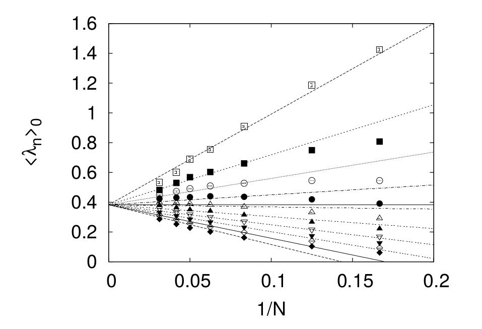
Refer to caption
Figure 5.3: Plot of the eigenvalues of Iμνsubscript𝐼𝜇𝜈I_{\mu\nu} against 1/N1𝑁1/N for the phase quenched IKKT model. From the figure it is clear that all the eigenvalues converge to a single point. This figure is taken from the Ref. [Anagnostopoulos 15].

5.2.3 Results

Due to lack of time during the final phase of the project, we were not able to produce the results for the full IKKT model. We are expecting the results provided in the Ref. [Anagnostopoulos 15]. Fig. 5.3 shows the result given in the Ref. [Anagnostopoulos 15]. In the limit N𝑁N\rightarrow\infty eigenvalues converge to a single point, which clearly shows that there is no SO(10)𝑆𝑂10SO(10) SSB in the phase quenched IKKT model.

Recent work on this model using complex Langevin algorithm showed that there is SSB of SO(10)𝑆𝑂10SO(10) to SO(3)×SO(7)𝑆𝑂3𝑆𝑂7SO(3)\times SO(7). (See Ref. [Anagnostopoulos 20].) In their paper, they further concluded that SO(7)𝑆𝑂7SO(7) symmetry is also broken.

Chapter 6 Conclusion and Future Work

The goal of this thesis is to study the bosonic BFSS model and the IKKT model using Monte Carlo simulations.

In the BFSS model we used Polyakov loop as an order parameter to investigate the large-N𝑁N behaviour of this model at different temperatures. We clearly observed the confinement-deconfinement phase transition in the quenched form of this model. From the energy vs temperature plot given in Ref. [Filev 16] it is clear that the phase transition is of second order. All our results are in excellent agreement with the results produced by other authors.

In the bosonic IKKT model we studied the spontaneous symmetry breaking (SSB) of SO(10)𝑆𝑂10SO(10) symmetry using the eigenvalues of the moment of inertia tensor and found that the system does not undergo SSB in the bosonic model. This directly suggests that dynamical compactification of extra dimensions is not possible in the bosonic IKKT model. We also tried to study the phase-quenched IKKT model but did not get enough time simulate it. In the future, we can study the phase-quenched IKKT model using RHMC algorithm and full IKKT model using complex Langevin with stochastic quantization. These studies have been carried out in Refs. [Ambjørn 00, Anagnostopoulos 20].

Appendix A Dimensional Reduction

This appendix provides an introduction on how to obtain the action of certain theories by dimensionally reducing from higher dimensions to lower dimensions using Kaluza-Klein compactification. We will also talk about Wick rotation, using which one can go from the Lorentzian field theory to the Euclidean one and vice-versa.

We will discuss how to dimensionally reduce the 𝒩=1𝒩1\mathcal{N}=1 super Yang-Mills theory in 9+1919+1 dimensions to 0+1010+1 dimensions and to 0+0000+0 dimension. In between we will also discuss the process of Wick rotation. The metric is given by ημν=diag(1,1,1,,1)subscript𝜂𝜇𝜈diag1111\eta_{\mu\nu}=\textrm{diag}(1,-1,-1,\cdots,-1). The action of the 𝒩=1𝒩1\mathcal{N}=1 super Yang-Mills theory in 9+1919+1 dimensions with gauge group SU(N)𝑆𝑈𝑁SU(N) is

S=d10x{12g102Tr(FμνFμν+2iΨ¯αγαβμDμΨβ)},𝑆superscript𝑑10𝑥12subscriptsuperscript𝑔210tracesubscript𝐹𝜇𝜈superscript𝐹𝜇𝜈2𝑖subscript¯Ψ𝛼subscriptsuperscript𝛾𝜇𝛼𝛽subscript𝐷𝜇subscriptΨ𝛽\displaystyle S=\int d^{10}x\,\left\{-\frac{1}{2g^{2}_{10}}\,\Tr(F_{\mu\nu}F^{\mu\nu}+2i\bar{\Psi}_{\alpha}\gamma^{\mu}_{\alpha\beta}D_{\mu}\Psi_{\beta})\right\}, (A.1)

where the integral for the temporal direction is from 00 to t0subscript𝑡0t_{0}. We have

DμΨβ=subscript𝐷𝜇subscriptΨ𝛽absent\displaystyle D_{\mu}\Psi_{\beta}= μΨi[Aμ,Ψβ],subscript𝜇Ψ𝑖subscript𝐴𝜇subscriptΨ𝛽\displaystyle\partial_{\mu}\Psi-i[A_{\mu},\Psi_{\beta}], (A.2)
Fμν=subscript𝐹𝜇𝜈absent\displaystyle F_{\mu\nu}= [μAν]i[Aμ,Aν],\displaystyle\partial_{[\mu}A_{\nu]}-i[A_{\mu},A_{\nu}], (A.3)

where μ,ν=0,1,2,,9formulae-sequence𝜇𝜈0129\mu,\nu=0,1,2,\cdots,9; α,β=1,2,,32formulae-sequence𝛼𝛽1232\alpha,\beta=1,2,\cdots,32; g10subscript𝑔10g_{10} is the coupling constant in 9+1919+1 dimensions; ΨΨ\Psi is the Majorana-Weyl fermion in 9+1919+1 dimensions with 32 components and each component is an N×N𝑁𝑁N\times N traceless Hermitian matrix. ΨΨ\Psi is in the adjoint representation of SU(N)𝑆𝑈𝑁SU(N), which is clear from the form of the covariant derivative Dμsubscript𝐷𝜇D_{\mu}. The above action, Eq. A.1, is invariant under the following gauge transformations

Aμ(x)subscript𝐴𝜇𝑥absent\displaystyle A_{\mu}(x)\rightarrow V(x)(Aμ(x)+iμ)V(x),𝑉𝑥subscript𝐴𝜇𝑥𝑖subscript𝜇superscript𝑉𝑥\displaystyle V(x)\,(A_{\mu}(x)+i\partial_{\mu})\,V^{\dagger}(x), (A.4)
Ψα(x)subscriptΨ𝛼𝑥absent\displaystyle\Psi_{\alpha}(x)\rightarrow V(x)Ψα(x)V(x).𝑉𝑥subscriptΨ𝛼𝑥superscript𝑉𝑥\displaystyle V(x)\,\Psi_{\alpha}(x)\,V^{\dagger}(x). (A.5)

The path integral for this system is given by

Z=𝒟Aμ𝒟Ψexp(iS).𝑍𝒟subscript𝐴𝜇𝒟Ψ𝑖𝑆\displaystyle Z=\int\mathcal{D}A_{\mu}\,\,\mathcal{D}\Psi\,\exp{iS}. (A.6)

Now we will apply the Kaluza-Klein compactification to dimensionally reduce this theory to lower dimensions. The idea of the Kaluza-Klein compactification is not to treat the dimension as of infinite length but rather compactify the dimension on the circle by introducing periodicity in this length dimension. For example, suppose there is only one spatial dimension and the objects repeat in this dimension after every 2πR2𝜋𝑅2\pi R distance. So it is clear that if we are close enough we will not be able to distinguish it from a line of infinite length but if we move far enough than we can clearly see that it is a circle of finite circumference. So if we want to compactify one dimension then we need to identify points after every 2πR2𝜋𝑅2\pi R distance and then take the limit R0𝑅0R\rightarrow 0. In the limit R0𝑅0R\rightarrow 0 with finite energy system, all the fields become independent of the coordinate of that dimension - see Ref. [Zwiebach 04]. The derivative in that direction no longer makes sense and all the derivative terms from the action disappears and component of the vector along that direction becomes a scalar.

Let us summarize how things change after compactification. Let us say we want to compactify along direction x9subscript𝑥9x_{9}. Then

ϕ(x0,x1,,x9)italic-ϕsubscript𝑥0subscript𝑥1subscript𝑥9absent\displaystyle\phi(x_{0},x_{1},\cdots,x_{9})\rightarrow ϕ(x0,x1,,x8),italic-ϕsubscript𝑥0subscript𝑥1subscript𝑥8\displaystyle\,\,\phi(x_{0},x_{1},\cdots,x_{8}), (A.7)
9ϕ(x)subscript9italic-ϕ𝑥absent\displaystyle\partial_{9}\phi(x)\rightarrow   0,  0\displaystyle\,\,0, (A.8)
A9(x0,x1,,x9)superscript𝐴9subscript𝑥0subscript𝑥1subscript𝑥9absent\displaystyle A^{9}(x_{0},x_{1},\cdots,x_{9})\rightarrow X9(x0,x1,,x8)(Scalar field).subscript𝑋9subscript𝑥0subscript𝑥1subscript𝑥8(Scalar field)\displaystyle\,\,X_{9}(x_{0},x_{1},\cdots,x_{8})\quad\textrm{(Scalar field)}. (A.9)

Now let us compactify the direction x9subscript𝑥9x_{9} on 𝐒1superscript𝐒1\mathbf{S}^{1} of radius R𝑅R for the action Eq. A.1. So A9(x)superscript𝐴9𝑥A^{9}(x) will be changed to X9(x)subscript𝑋9𝑥X_{9}(x) (Scalar field) and 9\partial_{9}\cdot will vanish. So F9νsubscript𝐹9𝜈F_{9\nu} and D9Ψβsubscript𝐷9subscriptΨ𝛽D_{9}\Psi_{\beta} will become

F9ν=subscript𝐹9𝜈absent\displaystyle F_{9\nu}= νX9+i[X9,Aν] where ν=0,1,,8,formulae-sequencesubscript𝜈subscript𝑋9𝑖subscript𝑋9subscript𝐴𝜈 where 𝜈018\displaystyle\partial_{\nu}X_{9}+i[X_{9},A_{\nu}]\qquad\textrm{ where }\nu=0,1,\cdots,8,
F9ν=subscript𝐹9𝜈absent\displaystyle F_{9\nu}= DνX9,F9ν=DνX9,subscript𝐷𝜈subscript𝑋9superscript𝐹9𝜈superscript𝐷𝜈subscript𝑋9\displaystyle D_{\nu}X_{9},\qquad F^{9\nu}=-D^{\nu}X_{9}, (A.10)
D9Ψβ=subscript𝐷9subscriptΨ𝛽absent\displaystyle D_{9}\Psi_{\beta}= i[X9,Ψβ].𝑖subscript𝑋9subscriptΨ𝛽\displaystyle i[X_{9},\Psi_{\beta}]. (A.11)

Substituting these back into the action we get

S=𝑆absent\displaystyle S= dx9d9x{12g102\displaystyle\int dx_{9}\,\int d^{9}x\,\Big{\{}-\frac{1}{2g^{2}_{10}}\,}
=\displaystyle= dx9d9x{12g102\displaystyle\int dx_{9}\,\int d^{9}x\,\Big{\{}-\frac{1}{2g^{2}_{10}}\,}
=\displaystyle= 2πRd9x{12g102\displaystyle 2\pi R\,\int d^{9}x\,\Big{\{}-\frac{1}{2g^{2}_{10}}\,}.

This gives

S9=subscript𝑆9absent\displaystyle S_{9}= d9x{12g92\displaystyle\int d^{9}x\,\Big{\{}-\frac{1}{2g^{2}_{9}}\,},

where

12g92=πRg102,12superscriptsubscript𝑔92𝜋𝑅subscriptsuperscript𝑔210\frac{1}{2g_{9}^{2}}=\frac{\pi R}{g^{2}_{10}}, (A.12)

and μ,ν= 0,1,,8formulae-sequence𝜇𝜈 018\mu,\,\nu=\,0,1,\cdots,8. Equation (A) is the action of the theory after compactifying x9subscript𝑥9x_{9} direction. Further, we notice that the coupling constant also changes. Now we will compactify the x8subscript𝑥8x_{8} direction on 𝐒1superscript𝐒1\mathbf{S}^{1} of radius R𝑅R. The following changes take place in the action

F8ν=subscript𝐹8𝜈absent\displaystyle F_{8\nu}= DνX8,F8ν=DνX8 where ν=0,1,,7,formulae-sequencesubscript𝐷𝜈subscript𝑋8superscript𝐹8𝜈superscript𝐷𝜈subscript𝑋8 where 𝜈017\displaystyle D_{\nu}X_{8},\quad F^{8\nu}=-D^{\nu}X_{8}\qquad\textrm{ where }\nu=0,1,\cdots,7, (A.13)
D8X9D8X9=subscript𝐷8subscript𝑋9superscript𝐷8subscript𝑋9absent\displaystyle D_{8}X_{9}D^{8}X_{9}= [X8,X9]2,superscriptsubscript𝑋8subscript𝑋92\displaystyle[X_{8},X_{9}]^{2}, (A.14)
D8Ψβ=subscript𝐷8subscriptΨ𝛽absent\displaystyle D_{8}\Psi_{\beta}= i[X8,Ψβ],𝑖subscript𝑋8subscriptΨ𝛽\displaystyle i[X_{8},\Psi_{\beta}], (A.15)
12g82=12superscriptsubscript𝑔82absent\displaystyle\frac{1}{2g_{8}^{2}}= πRg92.𝜋𝑅subscriptsuperscript𝑔29\displaystyle\frac{\pi R}{g^{2}_{9}}. (A.16)

The action becomes

S8=d8xsubscript𝑆8superscript𝑑8𝑥\displaystyle S_{8}=\int d^{8}x\, {12g82\displaystyle\Bigg{\{}-\frac{1}{2g^{2}_{8}}\,},

where μ,ν= 0,1,,7formulae-sequence𝜇𝜈 017\mu,\,\nu=\,0,1,\cdots,7. Now we can clearly see the pattern here. If we compactify one more spatial direction, say x7subscript𝑥7x_{7}, then we have

i=89DμXiDμXisuperscriptsubscript𝑖89subscript𝐷𝜇subscript𝑋𝑖superscript𝐷𝜇subscript𝑋𝑖\displaystyle\sum\limits_{i=8}^{9}D_{\mu}X_{i}D^{\mu}X_{i} i=79DμXiDμXi,absentsuperscriptsubscript𝑖79subscript𝐷𝜇subscript𝑋𝑖superscript𝐷𝜇subscript𝑋𝑖\displaystyle\to\sum\limits_{i=7}^{9}D_{\mu}X_{i}D^{\mu}X_{i}, (A.17)
i,j=8j>i9[Xi,Xj]2superscriptsubscript𝑖𝑗8𝑗𝑖9superscriptsubscript𝑋𝑖subscript𝑋𝑗2\displaystyle\sum\limits_{\begin{subarray}{c}i,j=8\\ j>i\end{subarray}}^{9}[X_{i},X_{j}]^{2} i,j=7j>i9[Xi,Xj]2,absentsuperscriptsubscript𝑖𝑗7𝑗𝑖9superscriptsubscript𝑋𝑖subscript𝑋𝑗2\displaystyle\to\sum\limits_{\begin{subarray}{c}i,j=7\\ j>i\end{subarray}}^{9}[X_{i},X_{j}]^{2}, (A.18)
i=89Ψ¯αγαβi[Xi,Ψβ]superscriptsubscript𝑖89subscript¯Ψ𝛼subscriptsuperscript𝛾𝑖𝛼𝛽subscript𝑋𝑖subscriptΨ𝛽\displaystyle\sum\limits_{i=8}^{9}\bar{\Psi}_{\alpha}\gamma^{i}_{\alpha\beta}[X_{i},\Psi_{\beta}] i=79Ψ¯αγαβi[Xi,Ψβ].absentsuperscriptsubscript𝑖79subscript¯Ψ𝛼subscriptsuperscript𝛾𝑖𝛼𝛽subscript𝑋𝑖subscriptΨ𝛽\displaystyle\to\sum\limits_{i=7}^{9}\bar{\Psi}_{\alpha}\gamma^{i}_{\alpha\beta}[X_{i},\Psi_{\beta}]. (A.19)

Applying this till we reach 0+1010+1 dimensions, the theory gets dimensionally reduced to a theory in 0+1010+1 dimensions. The action of this theory is given by

S1=subscript𝑆1absent\displaystyle S_{1}= 12g120t0𝑑tTr(2(DtXi)2[Xi,Xj]2+2iΨ¯αγαβ0DtΨβ2Ψ¯αγαβi[Xi,Ψβ]missing)12subscriptsuperscript𝑔21superscriptsubscript0subscript𝑡0differential-d𝑡trace2superscriptsubscript𝐷𝑡subscript𝑋𝑖2superscriptsubscript𝑋𝑖subscript𝑋𝑗22𝑖subscript¯Ψ𝛼subscriptsuperscript𝛾0𝛼𝛽subscript𝐷𝑡subscriptΨ𝛽2subscript¯Ψ𝛼subscriptsuperscript𝛾𝑖𝛼𝛽subscript𝑋𝑖subscriptΨ𝛽missing\displaystyle-\frac{1}{2g^{2}_{1}}\int\limits_{0}^{t_{0}}dt\,\Tr\Bigg(-2(D_{t}X_{i})^{2}-[X_{i},X_{j}]^{2}+2i\bar{\Psi}_{\alpha}\gamma^{0}_{\alpha\beta}D_{t}\Psi_{\beta}-2\bar{\Psi}_{\alpha}\gamma^{i}_{\alpha\beta}[X_{i},\Psi_{\beta}]\Bigg{missing})
=\displaystyle= 1g20t0𝑑tTr(12(DtXi)2+14[Xi,Xj]2i2Ψ¯αγαβ0DtΨβ+12Ψ¯αγαβi[Xi,Ψβ]missing),1superscript𝑔2superscriptsubscript0subscript𝑡0differential-d𝑡trace12superscriptsubscript𝐷𝑡subscript𝑋𝑖214superscriptsubscript𝑋𝑖subscript𝑋𝑗2𝑖2subscript¯Ψ𝛼subscriptsuperscript𝛾0𝛼𝛽subscript𝐷𝑡subscriptΨ𝛽12subscript¯Ψ𝛼subscriptsuperscript𝛾𝑖𝛼𝛽subscript𝑋𝑖subscriptΨ𝛽missing\displaystyle\frac{1}{g^{2}}\int\limits_{0}^{t_{0}}dt\,\Tr\Bigg(\frac{1}{2}(D_{t}X_{i})^{2}+\frac{1}{4}[X_{i},X_{j}]^{2}-\frac{i}{2}\bar{\Psi}_{\alpha}\gamma^{0}_{\alpha\beta}D_{t}\Psi_{\beta}+\frac{1}{2}\bar{\Psi}_{\alpha}\gamma^{i}_{\alpha\beta}[X_{i},\Psi_{\beta}]\Bigg{missing}), (A.20)

where 2g12=1g22superscriptsubscript𝑔121superscript𝑔2\frac{2}{g_{1}^{2}}=\frac{1}{g^{2}}, i,j= 1,2,,9formulae-sequence𝑖𝑗129i,j\,=\,1,2,\cdots,9 and repeated indices are summed over. Since ΨΨ\Psi is a Majorana fermion so we can use Ψ¯=ΨTC10¯ΨsuperscriptΨ𝑇subscript𝐶10\bar{\Psi}=\Psi^{T}C_{10}. Then the action becomes

S=𝑆absent\displaystyle S= 12g20t0𝑑tTr((DtXi)2+12[Xi,Xj]2iΨαTC10γαβ0DtΨβ+ΨαTC10γαβi[Xi,Ψβ]missing).12superscript𝑔2superscriptsubscript0subscript𝑡0differential-d𝑡tracesuperscriptsubscript𝐷𝑡subscript𝑋𝑖212superscriptsubscript𝑋𝑖subscript𝑋𝑗2𝑖subscriptsuperscriptΨ𝑇𝛼subscript𝐶10subscriptsuperscript𝛾0𝛼𝛽subscript𝐷𝑡subscriptΨ𝛽subscriptsuperscriptΨ𝑇𝛼subscript𝐶10subscriptsuperscript𝛾𝑖𝛼𝛽subscript𝑋𝑖subscriptΨ𝛽missing\displaystyle\frac{1}{2g^{2}}\int\limits_{0}^{t_{0}}dt\,\Tr\Bigg((D_{t}X_{i})^{2}+\frac{1}{2}[X_{i},X_{j}]^{2}-i\Psi^{T}_{\alpha}C_{10}\gamma^{0}_{\alpha\beta}D_{t}\Psi_{\beta}+\Psi^{T}_{\alpha}C_{10}\gamma^{i}_{\alpha\beta}[X_{i},\Psi_{\beta}]\Bigg{missing}). (A.21)

Equation (A.21) represents the action of the BFSS matrix model (see Ref. [Filev 16]).

Now we use Wick rotation to go from the Lorentzian action to the Euclidean action. Under Wick rotation the following changes take place

t𝑡absent\displaystyle t\to τ=it,𝜏𝑖𝑡\displaystyle\,\tau=it, (A.22)
dt𝑑𝑡absent\displaystyle dt\to dτ=idt,𝑑𝜏𝑖𝑑𝑡\displaystyle\,d\tau=idt, (A.23)
tsubscript𝑡absent\displaystyle\partial_{t}\to τ=it,subscript𝜏𝑖subscript𝑡\displaystyle\,\partial_{\tau}=-i\partial_{t}, (A.24)
A(t)𝐴𝑡absent\displaystyle A(t)\to A(τ)=iA(t).𝐴𝜏𝑖𝐴𝑡\displaystyle\,A(\tau)=-iA(t). (A.25)

Path integral changes to the partition function with β=it0𝛽𝑖subscript𝑡0\beta=it_{0} and the action changes to the Euclidean action. We take the representation of gamma matrices and C10subscript𝐶10C_{10} apart from γ0superscript𝛾0\gamma^{0} given in Ref. [Filev 16]. We take the following choice for the Majorana-Weyl fermion and γ0superscript𝛾0\gamma^{0}

Ψ=Ψabsent\displaystyle\Psi= ψ(10),tensor-product𝜓matrix10\displaystyle\psi\otimes\begin{pmatrix}1\\ 0\end{pmatrix}, (A.26)
γ0=superscript𝛾0absent\displaystyle\gamma^{0}= Γ10σ2.tensor-productsuperscriptΓ10subscript𝜎2\displaystyle\Gamma^{10}\otimes\sigma_{2}. (A.27)

Taking these things in account, the action and the path integral becomes

Z=𝒟Aτ𝒟X𝒟Ψexp(SE).𝑍𝒟subscript𝐴𝜏𝒟𝑋𝒟Ψsubscript𝑆E\displaystyle Z=\int\mathcal{D}A_{\tau}\,\,\mathcal{D}X\,\,\mathcal{D}\Psi\,\exp{-S_{\rm E}}. (A.28)
SE=12g20β𝑑τTr((DτXi)212[Xi,Xj]2iψαTC9Γαβ10DτψβψαTC9Γαβi[Xi,ψβ]),subscript𝑆E12superscript𝑔2superscriptsubscript0𝛽differential-d𝜏tracesuperscriptsubscript𝐷𝜏subscript𝑋𝑖212superscriptsubscript𝑋𝑖subscript𝑋𝑗2𝑖subscriptsuperscript𝜓𝑇𝛼subscript𝐶9subscriptsuperscriptΓ10𝛼𝛽subscript𝐷𝜏subscript𝜓𝛽subscriptsuperscript𝜓𝑇𝛼subscript𝐶9subscriptsuperscriptΓ𝑖𝛼𝛽subscript𝑋𝑖subscript𝜓𝛽\displaystyle S_{\rm E}=\frac{1}{2g^{2}}\int\limits_{0}^{\beta}d\tau\,\Tr((D_{\tau}X_{i})^{2}-\frac{1}{2}[X_{i},X_{j}]^{2}-i\psi^{T}_{\alpha}C_{9}\Gamma^{10}_{\alpha\beta}D_{\tau}\psi_{\beta}-\psi^{T}_{\alpha}C_{9}\Gamma^{i}_{\alpha\beta}[X_{i},\psi_{\beta}]), (A.29)

where Dτ=τi[A(τ),]subscript𝐷𝜏subscript𝜏𝑖𝐴𝜏D_{\tau}=\partial_{\tau}-i[A(\tau),\cdot]; α,β=1,2,,16formulae-sequence𝛼𝛽1216\alpha,\,\beta=1,2,\cdots,16; i,j=1,2,,9formulae-sequence𝑖𝑗129i,\,j=1,2,\cdots,9; C9subscript𝐶9C_{9} is the 9-dimensional Euclidean charge conjugation matrix; ΓisuperscriptΓ𝑖\Gamma^{i} are the Euclidean gamma matrices in 9 dimensions. Bosonic fields follow periodic boundary conditions, i.e., A(τ+β)=A(τ)𝐴𝜏𝛽𝐴𝜏A(\tau+\beta)=A(\tau) and Xi(τ+β)=Xi(τ)subscript𝑋𝑖𝜏𝛽subscript𝑋𝑖𝜏X_{i}(\tau+\beta)=X_{i}(\tau), and fermionic fields follow anti-periodic boundary conditions, i.e., ψ(τ+β)=ψ(τ)𝜓𝜏𝛽𝜓𝜏\psi(\tau+\beta)=-\psi(\tau). Eq. (A.29) represents the Euclidean action of the BFSS matrix model. This equation is used in Chapter 4.

If we dimensionally reduce the above model to 0+0000+0 dimensions, we will get the IKKT matrix model. The Euclidean action of IKKT matrix model is given by

SE=14g02Tr([Xi,Xj]2)12g02Tr(ψαTC9Γαβi[Xi,ψβ]),subscript𝑆E14superscriptsubscript𝑔02tracesuperscriptsubscript𝑋𝑖subscript𝑋𝑗212superscriptsubscript𝑔02tracesubscriptsuperscript𝜓𝑇𝛼subscript𝐶9subscriptsuperscriptΓ𝑖𝛼𝛽subscript𝑋𝑖subscript𝜓𝛽\displaystyle S_{\rm E}=-\frac{1}{4g_{0}^{2}}\Tr([X_{i},X_{j}]^{2})-\frac{1}{2g_{0}^{2}}\Tr(\psi^{T}_{\alpha}C_{9}\Gamma^{i}_{\alpha\beta}[X_{i},\psi_{\beta}]), (A.30)

where g0subscript𝑔0g_{0} is the 0-dimensional Yang-Mills coupling,i,j=1,2,,10formulae-sequence𝑖𝑗1210i\,,j=1,2,\cdots,10. This equation is used in Chapter 5.

Bibliography

  • [Ambjørn 00] Jan Ambjørn, Jun Nishimura, Konstantinos N Anagnostopoulos, Wolfgang Bietenholz & Tomohiro Hotta. Monte Carlo studies of the IIB matrix model at large N. Journal of High Energy Physics, vol. 2000, no. 07, page 011–011, Jul 2000.
  • [Anagnostopoulos 15] Konstantinos N. Anagnostopoulos, Takehiro Azuma & Jun Nishimura. Monte Carlo studies of dynamical compactification of extra dimensions in a model of nonperturbative string theory, 2015.
  • [Anagnostopoulos 20] Konstantinos N. Anagnostopoulos, Takehiro Azuma, Yuta Ito, Jun Nishimura, Toshiyuki Okubo & Stratos Kovalkov Papadoudis. Complex Langevin analysis of the spontaneous breaking of 10D rotational symmetry in the Euclidean IKKT matrix model, 2020.
  • [Aoki 98] H. Aoki, S. Iso, H. Kawai, Y. Kitazawa & T. Tada. Space-Time Structures from IIB Matrix Model. Progress of Theoretical Physics, vol. 99, no. 5, page 713–745, May 1998.
  • [Banks 97] Tom Banks, Willy Fischler, Steven H Shenker & Leonard Susskind. M theory as a matrix model: A conjecture. Physical Review D, vol. 55, no. 8, page 5112, 1997.
  • [Banks 98] Tom Banks, Willy Fischler, Igor R Klebanov & Leonard Susskind. Schwarzschild black holes in Matrix theory II. Journal of High Energy Physics, vol. 1998, no. 01, page 008, 1998.
  • [Betancourt 17] Michael Betancourt. A conceptual introduction to Hamiltonian Monte Carlo. arXiv preprint arXiv:1701.02434, 2017.
  • [Clark 05] M.A. Clark & A.D. Kennedy. https://github.com/mikeaclark/AlgRemez, 2005.
  • [Filev 16] Veselin G. Filev & Denjoe O’Connor. The BFSS model on the lattice. Journal of High Energy Physics, vol. 2016, no. 5, May 2016.
  • [Furuuchi 03] K. Furuuchi, E. Schreiber & G. W. Semenoff. Five-Brane Thermodynamics from the Matrix Model, 2003.
  • [Gattringer 09] Christof Gattringer & Christian B Lang. Quantum Chromodynamics on the Lattice: An Introductory Presentation (Lecture Notes in Physics Vol. 788), 2009.
  • [Hadizadeh 05] Shirin Hadizadeh, Bojan Ramadanovic, Gordon W Semenoff & Donovan Young. Free energy and phase transition of the matrix model on a plane wave. Physical Review D, vol. 71, no. 6, page 065016, 2005.
  • [Hanada 07] Masanori Hanada, Jun Nishimura & Shingo Takeuchi. Nonlattice Simulation for Supersymmetric Gauge Theories in One Dimension. Physical Review Letters, vol. 99, no. 16, Oct 2007.
  • [Hotta 99] Tomohiro Hotta, Jun Nishimura & Asato Tsuchiya. Dynamical aspects of large-N reduced models. Nuclear Physics B, vol. 545, no. 1-3, page 543–575, Apr 1999.
  • [Ishibashi 97] Nobuyuki Ishibashi, Hikaru Kawai, Yoshihisa Kitazawa & Asato Tsuchiya. A large-N reduced model as superstring. Nuclear Physics B, vol. 498, no. 1-2, page 467–491, Aug 1997.
  • [Ito 14] Y. Ito, S.-W. Kim, Y. Koizuka, J. Nishimura & A. Tsuchiya. A renormalization group method for studying the early universe in the Lorentzian IIB matrix model. Progress of Theoretical and Experimental Physics, vol. 2014, no. 8, page 83B01–0, Aug 2014.
  • [Ito 15] Yuta Ito, Jun Nishimura & Asato Tsuchiya. Power-law expansion of the Universe from the bosonic Lorentzian type IIB matrix model. Journal of High Energy Physics, vol. 2015, no. 11, Nov 2015.
  • [Joseph 15] Anosh Joseph. Review of lattice supersymmetry and gauge-gravity duality. International Journal of Modern Physics A, vol. 30, no. 27, page 1530054, Sep 2015.
  • [Joseph 20] Anosh Joseph. Markov chain monte carlo methods in quantum field theories: A modern primer. Springer, Cham, 2020.
  • [Kabat 01a] Daniel Kabat, Gilad Lifschytz & David Lowe. Black hole thermodynamics from calculations in strongly coupled gauge theory. International Journal of Modern Physics A, vol. 16, no. 05, pages 856–865, 2001.
  • [Kabat 01b] Daniel Kabat, Gilad Lifschytz & David A Lowe. Black hole entropy from nonperturbative gauge theory. Physical Review D, vol. 64, no. 12, page 124015, 2001.
  • [Kawahara 07a] Naoyuki Kawahara, Jun Nishimura & Shingo Takeuchi. High temperature expansion in supersymmetric matrix quantum mechanics. Journal of High Energy Physics, vol. 2007, no. 12, page 103–103, Dec 2007.
  • [Kawahara 07b] Naoyuki Kawahara, Jun Nishimura & Shingo Takeuchi. Phase structure of matrix quantum mechanics at finite temperature. Journal of High Energy Physics, vol. 2007, no. 10, page 097–097, Oct 2007.
  • [Klebanov 98] Igor R Klebanov & Leonard Susskind. Schwarzschild black holes in various dimensions from matrix theory. Physics Letters B, vol. 416, no. 1-2, pages 62–66, 1998.
  • [Metropolis 53] Nicholas Metropolis, Arianna W Rosenbluth, Marshall N Rosenbluth, Augusta H Teller & Edward Teller. Equation of state calculations by fast computing machines. The journal of chemical physics, vol. 21, no. 6, pages 1087–1092, 1953.
  • [Neal 11] Radford M Nealet al. MCMC using Hamiltonian dynamics. Handbook of markov chain monte carlo, vol. 2, no. 11, page 2, 2011.
  • [Nishimura 00] Jun Nishimura & Graziano Vernizzi. Brane World Generated Dynamically from String Type IIB Matrices. Physical Review Letters, vol. 85, no. 22, page 4664–4667, Nov 2000.
  • [Nishimura 11] Jun Nishimura, Toshiyuki Okubo & Fumihiko Sugino. Systematic study of the SO(10) symmetry breaking vacua in the matrix model for type IIB superstrings. Journal of High Energy Physics, vol. 2011, no. 10, Oct 2011.
  • [Nishimura 19] Jun Nishimura & Asato Tsuchiya. Complex Langevin analysis of the space-time structure in the Lorentzian type IIB matrix model. Journal of High Energy Physics, vol. 2019, no. 6, Jun 2019.
  • [Nishimura 20] Jun Nishimura. New perspectives on the emergence of (3+1)D expanding space-time in the Lorentzian type IIB matrix model, 2020.
  • [Peskin 95] Michael E Peskin & Daniel V Schroeder. An Introduction to Quantum Field Theory (Boulder, CO), 1995.
  • [Polyakov 78] Alexander M Polyakov. Thermal properties of gauge fields and quark liberation. Physics Letters B, vol. 72, no. 4, pages 477–480, 1978.
  • [Robert 04] Christian Robert & George Casella. Monte carlo statistical methods springer-verlag. New York, 2004.
  • [SEMENOFF 04] GORDON W. SEMENOFF. MATRIX MODEL THERMODYNAMICS. Quantum Theory and Symmetries, Oct 2004.
  • [Vetterling 02] William T Vetterling, William H Press, Saul A Teukolsky & Brian P Flannery. Numerical recipes example book (c++): The art of scientific computing. Cambridge University Press, 2002.
  • [Wilson 74] Kenneth G Wilson. Confinement of quarks. Physical review D, vol. 10, no. 8, page 2445, 1974.
  • [Witten 95] Edward Witten. String theory dynamics in various dimensions. Nuclear Physics B, vol. 443, no. 1-2, page 85–126, Jun 1995.
  • [Ydri 17] Badis Ydri. Computational Physics: An Introduction to Monte Carlo Simulations of Matrix Field Theory. World Scientific, Singapore, 2017.
  • [Zee 10] Anthony Zee. Quantum field theory in a nutshell, volume 7. Princeton university press, 2010.
  • [Zwiebach 04] Barton Zwiebach. A first course in string theory. Cambridge university press, 2004.