Compressing Deep Neural Networks via Layer Fusion

Abstract

This paper proposes layer fusion - a model compression technique that discovers which weights to combine and then fuses weights of similar fully-connected, convolutional and attention layers. Layer fusion can significantly reduce the number of layers of the original network with little additional computation overhead, while maintaining competitive performance. From experiments on CIFAR-10, we find that various deep convolution neural networks can remain within 2% accuracy points of the original networks up to a compression ratio of 3.33 when iteratively retrained with layer fusion. For experiments on the WikiText-2 language modelling dataset where pretrained transformer models are used, we achieve compression that leads to a network that is 20% of its original size while being within 5 perplexity points of the original network. We also find that other well-established compression techniques can achieve competitive performance when compared to their original networks given a sufficient number of retraining steps. Generally, we observe a clear inflection point in performance as the amount of compression increases, suggesting a bound on the amount of compression that can be achieved before an exponential degradation in performance.

Introduction

Deep neural networks (DNNs) have made a significant impact in fields such as Computer Vision (CV) (?; ?) and Natural Language Processing (NLP)  (?; ?). This has been accelerated due to numerous innovations. For example, Residual Networks (ResNets)  (?), that are often employed in CV, use skip connections to avoid the vanishing gradient problem in very deep networks, while batch normalization  (?; ?) and layer normalization (?) are used to reduce the effects of shifts in the training and test data distributions. Tangentially for NLP, Transformer networks have shown great success due to the use of self-attention (?). Transformers have shown significant performance improvements over Recurrent Neural Networks with internal memory (RNNs) (?) for sentence representations, language modelling and conditional text generation (?; ?; ?) and various other natural language understanding (NLU) tasks. Similarly, deep Convolutional Neural Networks (CNNs) (?) have improved performance on image classification (?), image segmentation (?), speech recognition (?) and been widely adopted in the machine learning (ML) community. However, large overparameterized networks require more compute, training time, storage and leave a larger carbon footprint (?). Previous work on model compression has mainly focused on deploying compressed models to mobile devices (?; ?). However, moving models from multi-GPU training to single-GPU training is now too a salient challenge, in order to relax the resource requirements for ML practitioners and allow a wider adoption of larger pretrained CNNs and Transformers within the community. DNNs becoming increasingly deeper leads us to ask the following questions: are all layers of large pretrained models necessary for a given target task ? If not, can we reduce the network while preserving network density during retraining in a computationally efficient manner?. We are also motivated to fuse layers based on findings that show whole layers can be distinctly separated by their importance in prediction (?). Earlier work on CNNs found that some layers may become redundant in very deep networks (?), essentially copying earlier layers and performing identity mappings for the redundant layers. While residual connections have ameliorated these problems to some degree (not only in residual networks e.g Transformers), we assert that there may still be significant overlap between layers of large overparameterized networks.

Guided by Occam’s razor (?), one can use various compression techniques (e.g pruning, tensor decomposition, knowledge distillation, quantization) post-training to find smaller networks from pretrained models. However, many of the existing compression techniques are unstructured (?; ?; ?), resulting in a sparse model. This is a practical limitation since sparse networks require more conditional operations to represent which elements within each parameter matrix are zero or non-zero. Current GPU libraries such as CuSPARSE (accounting for recent improvements (?)) are far slower than CuBLAS (?) and fundamentally, current hardware is not designed to optimize for sparse matrix operations. In contrast, knowledge distillation (?; ?; ?), and quantization (?) preserve network density, avoiding the necessity for specialized sparse matrix libraries to utilize the benefits of smaller and faster networks. However, quantization leads to quantization error and requires approximate methods to compute partial derivatives during retraining (?) and knowledge distillation requires more memory to store and train the smaller network. Weight sharing reduces the network size and avoids sparsity, however it is unclear which weights should be shared and it cannot be used when the model is already pretrained with untied weights. The noted drawbacks of the aforementioned compression methods further motivates to seek an alternative structured compression method that preserves network density while identifying and removing redundancy in the layers. This brings us to our main contributions.

Contributions

We propose layer fusion (LF). LF aims to preserve information across layers during retraining of already learned models while preserving layer density for computational efficiency. Since aligning paths, layers and whole neural networks is non-trivial (neurons can be permuted and still exhibit similar behaviour and we desire an invariance to orthogonal transformations), we also propose alignment measures for LF. This includes (1) a Wasserstein distance metric to approximate the alignment cost between weight matrices and (2) numerous criteria for measuring similarity between weight covariance matrices. We use these measures as LF criteria to rank layer pairs that are subsequently used to fuse convolutional, fully-connected and attention layers. This leads to both computational and performance improvements over layer removal techniques, network pruning and shows competitive results compared to tensor-decomposition and unsupervised-based knowledge distillation. In our experiments, we report LF using different fusion approaches: layer freezing, averaging and random mixing. Lastly, we report results on using structured compression for large pretrained transformers and CNNs and provide experimental results of different compression methods with and without retraining. Thus, we identify the importance of retraining pretrained models.

Related Work

Layer Structure & Importance

? (?) have recently analysed the layer-wise functional structure of overparameterized deep models to gain insight into why deep networks have performance advantages over their shallow counterparts. They find that some layers are salient and that once removed, or reinitialized, have a catastrophic effect on learning during training and subsequently generalization. In contrast, the remaining layers once reset to their default initialization has little effect. This suggests that parameter and norm counting is too broad of a measure to succinctly study the generalization properties in deep networks. These findings also motivate LF, as we posit that important layers are more distinct and therefore will be less similar, or harder to align with other layers, while more redundant layers may be good candidates for fusing layers.

Recently, ? (?) empirically showed that there exists trained subnetworks that when re-initialized to their original configuration produce the same performance as the original network in the same number of training epochs. They also posit that stochastic gradient descent (SGD) seeks out a set of lottery tickets (i.e well-initialized weights that make up a subnetwork that when trained for the same number of epochs as the original network, or less, can reach the same out-of-sample performance) and essentially ignores the remaining weights. We can further conjecture from ? (?) findings, that perhaps SGD more generally seeks out important layers, which we analogously refer to as lottery pools. Identifying whole layers that are significantly distinguished from others, in terms of their influence on learning, further motivates us to pursue the merging or freezing of layers in DNNs.

Computing Layer Similarity

? (?) have focused on computing similarity between different neural representations (i.e the activation output vector for a given layer). However, we view this comparison between layers as slightly limiting, since information is lost about what weights and bias led to the activation outputs. Moreover, directly comparing neural network weights allows us to avoid sampling inputs to compute the activations. In contrast, work focusing on representational similarity across networks ?; ? (?; ?), we are instead comparing weight matrices within the same network. Directly comparing weights and biases allow us to better approximate alignments and similarities for dense networks and has the advantage that we do not require data to be fed-forward through the network post-training to measure similarity within or across networks, unlike representational similarity (i.e output activations).

Structured Dropout ? (?) proposes to randomly drop whole layers during training time and at test time they can choose a subnetwork which can be decided based on performance of different combinations of pruned networks on the validation set or based on dropout probabilities learned for each layer throughout training.

? (?) measure model similarity across neural networks using optimal transport-based metrics. In contrast, our work measures intra-network similarity and we make a distributional assumption that allows us to use such metric to be used efficiently during retraining and to scale for large networks.

Methodology

Preliminaries We define a dataset as $\{D=(\vec{x}_{i},\vec{y}_{i}):i=1,\ldots T\}$ that contains $T$ tuples of an input vector $\vec{x}\in\mathbb{R}^{n}$ and a corresponding target $\vec{y}\in\{0,1\}^{p}$. We define any arbitary sample as $s:=(\vec{x},\vec{y})$ where $s\in D$. We consider a neural network $f_{\theta}(\vec{x})$ with pretrained parameters $\theta:=(\text{\bf W}_{1},\text{\bf W}_{2},\ldots\theta_{\ell}\ldots,\theta_{L})^{T}$. Here $\theta_{\ell}:=\{\text{\bf W}_{\ell},\vec{b}_{\ell}\}$ where $\text{\bf W}_{\ell}\in\mathbb{R}^{n_{\ell}\times n_{\ell+1}}$, $\vec{b}\in\mathbb{R}^{n_{\ell+1}}$ where $n_{\ell}$ denotes the dimension size of the $\ell$-th layer. Thus, a standard fully-connected $f_{\theta}$ is expressed as,

$$f_{\theta}(\vec{x}):=\text{\bf W}_{L}g\Big{(}\ldots g\big{(}\text{\bf W}_{2}g(\text{\bf W}_{1}\vec{x}+\vec{b}_{1}\big{)}+\vec{b}_{2}\Big{)}+\vec{b}_{L}$$ (1)

with smooth asymptotic nonlinear function $g(\cdot)$ (e.g hyperbolic tangent) that performs elementwise operations on its input. The input to each subsequent layer as $\vec{z}_{\ell}\in\mathbb{R}^{n_{\ell}}$ where $\vec{x}\coloneqq\vec{z}_{0}$ for $m$ number of units in layer ${\ell}$ and the corresponding output activation as $\vec{T}_{\ell}=g(\vec{z}_{\ell})$. The loss function is defined as $\mathbb{L}_{\theta}(D):=\frac{1}{T}\sum_{i=1}^{N}\mathcal{L}(\vec{y}_{i},f_{\theta}(\vec{x}_{i}))$ where for a single sample $s_{i}$, $\mathcal{L}:\mathcal{Y}\times\mathbb{R}^{n}\to\mathbb{R}$. A pruned $\theta_{\ell}$ post-training is denoted as $\theta^{p}_{\ell}$ and a tensor decomposed $\theta_{\ell}$ is expressed as $\tilde{\theta}_{\ell}$ where $\tilde{\text{\bf W}}_{\ell}\in\mathbb{R}^{d_{\ell}\times d_{\ell+1}}$ and $\tilde{\vec{b}}_{\ell}\in\mathbb{R}^{d_{\ell+1}}$ and $d\ll n$. A network pruned by layer as a percentage of the lowest weight magnitudes is denoted as $f^{lp}_{\acute{\theta}}$ where the pruned weights $\acute{\theta}\subset\theta$. A percentage of the network pruned by weight magnitudes across the whole network is denoted as $f^{gp}_{\acute{\theta}}$ (i.e global pruning). Lastly, a post layer fused network $f_{\Theta}$ has fused parameters $\Theta$.

Desirable Properties of a Layer Similarity Measure

Ideally, we seek a measure that can compare weight matrices that are permutable and of varying length. Formally, the main challenges with aligning weight matrices $\text{\bf W}:=\{\text{\bf W}_{0},\ldots,\text{\bf W}_{\ell},\ldots\text{\bf W}_{L}\}$ of different layers is that, when vectorized as $\mathtt{vec}(\text{\bf W}_{\ell})\in\mathbb{R}^{n_{\ell}(n_{\ell+1})}$, $\text{\bf W}_{\ell}$ can be permuted and still exhibit the same behavior at the output. Hence, if $|\text{\bf W}_{\ell}|\neq|\text{\bf W}_{\ell+1}|$, the measure $S$ must allow for multisets of different lengths and permutations. Invariance to rotations, reflections and scaling are all desirable properties we aim to incorporate into measuring similarity between weight matrices. However, invariance to linear transformations has issues when there are more parameters in a layer than training samples, as pointed out by ? (?). Eventhough our work mainly focuses on large pretrained models, we too seek a LF measure that is invariant to orthogonal transformations to overcome the aforementioned issues i.e for a similarity function $s(\cdot,\cdot)$, $s(\text{\bf W}_{i},\text{\bf W}_{j})=s(\text{\bf W}_{i}\text{\bf U},\text{\bf W}_{j}\text{\bf V})$ for full-rank orthonormal matrices U and V such that $\text{\bf U}^{T}\text{\bf U}=\text{\bf I}$ and $\text{\bf V}^{T}\text{\bf V}=\text{\bf I}$. More importantly, invariance to orthogonal transformation relates to permutation invariance (?) which is a property we account when measuring similarity to fuse weight matrices. We now describe a set of measures we consider for aligning and measuring the similarity of layers.

Layer Alignment & Layer Similarity

Covariance Alignment

The first layer fusion measure we consider is covariance alignment (CA). CA accounts for correlated intra-variant distances between layers, which can indicate some redundancy, although their overall distributions may differ and therefore may be good candidates for LF. Hence, we consider the Frobenius norm (denoted as subscript $F$) between pairs of weight covariance matrices $\vec{\Sigma}_{\tilde{\text{\bf W}}_{1}},\vec{\Sigma}_{\tilde{\text{\bf W}}_{2}}$ and expectation $\mathbb{E}[{\text{\bf W}}_{1}]=\mathbb{E}[{\text{\bf W}}_{2}]=0$. This forms a Riemannian manifold of non-positive curvature over the weight covariances. We first consider the cosine distance as the distance measures between parameter covariance matrices as Equation 2, where $||\Sigma_{\text{\bf W}}||_{F}=[\text{tr}(\Sigma_{\text{\bf W}}^{T}\Sigma_{\text{\bf W}})]^{1/2}$.

$$\text{cos}(\vec{\Sigma}_{\text{\bf W}_{1}},\vec{\Sigma}_{\text{\bf W}_{2}})=\frac{\mathop{tr}\big{(}\vec{\Sigma}_{\text{\bf W}_{1}}\cdot\vec{\Sigma}_{\text{\bf W}_{2}}\big{)}}{||\vec{\Sigma}_{\text{\bf W}_{1}}||_{F}||\vec{\Sigma}_{\text{\bf W}_{2}}||_{F}}$$ (2)

If we assume both weight matrices are drawn from a normal distribution $\text{\bf W}_{1}\sim\mathcal{N}(\mu,\sigma_{1}),\text{\bf W}_{2}\sim\mathcal{N}(\mu,\sigma_{2})$ with identical means $\mu=\mu_{\text{\bf W}_{1}}=\mu_{\text{\bf W}_{2}}$, the KL divergence between their covariance matrices can be expressed as:

$$\text{KL}(\mathbf{\Sigma}_{\text{\bf W}_{1}}||\mathbf{\Sigma}_{\text{\bf W}_{2}})=\frac{1}{2}\Big{[}\mathop{tr}\big{(}\vec{\Sigma}_{\text{\bf W}_{2}}^{-1}\vec{\Sigma}_{\text{\bf W}_{1}})-\ln\big{(}\frac{|\vec{\Sigma}_{\text{\bf W}_{1}}|}{|\vec{\Sigma}_{\text{\bf W}_{2}}|}\big{)}\Big{]}$$ (3)

The symmetrized KL divergence between positive semi-definite matrices (e.g covariances) also acts as the square of a distance (?) (see supplementary for further details, including descriptions of other covariance similarity measures). We consider both Equation 2 and Equation 3 for fusing convolutional layers, self-attention layers and fully-connected layers. The KL is an asymmetric measure, therefore the divergence in both directions can be used to assign a weight to each layer pair in layer fusion.

Optimal Transport & Wasserstein Distance

Unlike an all-pair distance such as CA, Wasserstein (WS) distance can also be used to find the optimal cost, also known as the optimal flow between two distributions. Unlike, other distance measures, WD tries to keep the geometry of the distributions intact when interpolating and measuring between distributions. Unlike CA and other baseline measures, WS is invariant to layer permutations and like CA, it also accounts for mutual dependencies between parameters in any arbitrary layer. In this work, we consider the WD between adjacent row-normalized parameter pairs $\text{softmax}(\text{\bf W}_{1},\text{\bf W}_{2})$ (i.e multisets) in a Euclidean metric space. Given two multi-sets $\text{\bf W}_{1},\text{\bf W}_{2}\subset\text{\bf W}$, of size $d=|\text{\bf W}_{1}|=|\text{\bf W}_{2}|$ with corresponding empirical distributions $P_{\text{\bf W}_{1}}$ and $P_{\text{\bf W}_{2}}$, the WS distance is defined as Equation 4. However, computing WS distance is $\mathcal{O}(N^{3})$ using the standard Hungarian algorithm, which is intractable for large $\theta$.

$$W_{p}(P_{\text{\bf W}_{1}},P_{\text{\bf W}_{2}})=\inf_{\pi}\Big{(}\sum_{i=1}^{d}||P_{\text{\bf W}_{1}^{i}}-P_{\text{\bf W}_{2}^{\pi(i)}}||^{p}\Big{)}^{1/p}$$ (4)

One way to tradeoff this computational burden is to assume that the weights are i.i.d and normally distributed at the expense of disregarding mutual dependencies learned throughout training. According to Lyapunov’s central limit theorem (?), we can assume the the weights in a layer are normally distributed. Hence, if $P_{\text{\bf W}_{1}}=N(\mu_{\text{\bf W}_{1}},\vec{\Sigma}_{1})$ and $P_{\text{\bf W}_{2}}=N(\mu_{\text{\bf W}_{2}},\vec{\Sigma}_{2})$ we can express the 2-WS distance as Equation 5, also known as the Bures metric.

$$\mathbb{W}^{2}(P_{\text{\bf W}_{1}},P_{\text{\bf W}_{2}})=||\mu_{\text{\bf W}_{1}}-\mu_{\text{\bf W}_{2}}||^{2}+\mathbb{B}^{2}(\vec{\Sigma}_{\text{\bf W}_{1}},\vec{\Sigma}_{\text{\bf W}_{2}}),$$ (5)

$$\mathbb{B}^{2}(\vec{\Sigma}_{\text{\bf W}_{1}},\vec{\Sigma}_{\text{\bf W}_{2}})=\text{tr}(\vec{\Sigma}_{\text{\bf W}_{1}})+\text{tr}(\vec{\Sigma}_{\text{\bf W}_{2}})-$$

$$2\text{tr}\Big{[}\big{(}\sqrt{\vec{\Sigma}_{\text{\bf W}_{1}}}(\vec{\Sigma}_{\text{\bf W}_{2}}\sqrt{\vec{\Sigma}_{\text{\bf W}_{1}}})\big{)}\Big{]}$$

Although we focus on the Bures metric in our experiments, an alternative approach is to find a set of cluster centroids in $\text{\bf W}_{1}$ and $\text{\bf W}_{2}$ as $C_{\text{\bf W}_{2}}$ and $C_{\text{\bf W}_{2}}$ and compute $W(P_{C_{\text{\bf W}_{1}}},P_{C_{\text{\bf W}_{2}}})$. In this approach the centroids are converted to an empirical distribution $P_{C_{\theta}}$ such $c\ll d$ such that a $\mathcal{O}(N^{3})$ cost is feasible for computing during retraining steps. Alternatively, we could avoid softmax normalization and directly compute $W(C_{\text{\bf W}_{1}},C_{\text{\bf W}_{2}})$ on both discrete sets. Lastly, we note that when fusing layers with 2-WS distance, the fusion occurs between aligned weights given by the cost matrix. Hence, it is not only used to identify top-k most similar layers, but the cost matrix also aligns which weights in the layer pair are fused.

Fusing Layers

After choosing the top-k layer pairs to merge, we then consider 3 ways to fuse the layers: (1) freeze one of the two layers (i.e do not compute gradients for one of the two layers), (2) take the mean between layer pairs and compute backprop on the averaged layer pair and (3) sample and mix between the layers. Choosing the layers to fuse for (1) is based on which of the two is closest to the middle layer of the network. This is motivated by previous work that showed layers closer to the input and output are generally more salient (?). When using Jenson-Shannon divergence for choosing top-k layers, we use the divergence asymmetry for choosing which layer is frozen. This is achieved by taking the parameter $\gamma$ between the Jenson-Shannon divergence of two layers in both directions to control a weighted gradient. We express the backpropogation when using LF with Jenson-Shannon divergence in terms of KL-divergences as shown in Equation 6, where $\bar{\text{\bf W}}_{ij}$ is a mixture distribution between ${\text{\bf W}}_{i}$ and ${\text{\bf W}}_{j}$ with a weighted gradient $\partial\mathcal{L}/\partial\tilde{\text{\bf W}}_{ij}$ that represents the gradient for both ${\text{\bf W}}_{i}$ and ${\text{\bf W}}_{j}$. Thus, for the backward pass of a frozen layer from a given top-k pair, we still compute its gradients which will influence how its original pair will be updated. This constraint ensures that the original pair that were most similar for a given compression step remain relatively close throughout retraining. The layer pair are then averaged at test time to reduce network size, while maintaining similarity using the aforementioned JS divergence gradient constraint.

$$\begin{gathered}\frac{\partial\mathcal{L}}{\partial\tilde{\text{\bf W}}_{ij}}:=\gamma\Big{(}\frac{\partial L}{\text{\bf W}_{i}}\Big{)}+\big{(}1-\gamma\big{)}\Big{(}\frac{\partial L}{\text{\bf W}_{j}}\Big{)}\quad s.t,\\ \gamma=\frac{1}{2}\Big{(}\text{KL}(\text{\bf W}_{i}||\bar{\text{\bf W}}_{ij})+\text{KL}(\text{\bf W}_{j}||\bar{\text{\bf W}}_{ij})\Big{)}\end{gathered}$$ (6)

For (2), updates during training when using , we constrain the gradients to be the average of both layers and then average the resulting layers at the end of retraining. For (3), we interpolate between hidden representations that are most similar, which can be viewed as a stochastic approach of JS divergence used in (1), to remove redundancy in the network. We denote a pair of randomly mixed layers as $\tilde{\text{\bf W}}^{i}_{\ell}\sim\mathbb{B}\big{(}\text{\bf W}^{i}_{\ell},\text{\bf W}_{\ell+1}\big{)}\quad\forall i\in n_{\ell}$. Note that we only mix between pairs of weight matrices, the bias terms are averaged $(\vec{b}_{\ell}+\vec{b}_{\ell})/2$. We then compute backpropogation on $\tilde{\theta}^{i}_{\ell}$ instead of the original unmixed layer pair $(\theta{i}_{\ell},\tilde{\theta}^{i}_{\ell+1})$ i.e mixing is carried out before the forward pass.

Experimental Details

We focus on transformer-based models for language modelling on the WikiText-2 dataset (?). For large models in NLP such as BERT (?), OpenAI-GPT, GPT2 (?) and Transformer-XL (?), we freeze or combine layer weights of each multi-attention head component and intermediate dense layers, dramatically reducing the respective number of layer and weights. For image classification on CIFAR10, we report results for ResNet, ResNet-ELU (?), Wide-ResNet (?) and DenseNet (?). We are particularly interested in ResNet architectures, or more generally, ones that also use skip connections. This is motivated by  ? (?) which found that deleting or permuting residual blocks can be carried out without much degradation in performance in a pretrained ResNet.

Compression Without Reraining

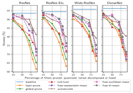
(a) No Retraining

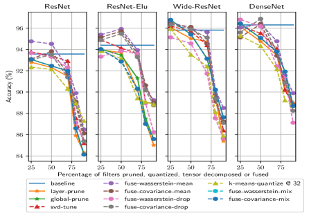
(b) Retraining

Figure 1: CIFAR-10 Test Accuracy with and without Retraining

For magnitude-based pruning, we prune a percentage of the weights with the lowest magnitude. This is done in one of two ways: a percentage of weights pruned by layer (layer pruning), or a percentage of the network as whole (global pruning). For quantization, we use k-means whereby the number of clusters for a given layer is specified as a percentage of the original size of that layer (i.e number of parameters in the tensor). For tensor decomposition, we reduce the number of parameters by approximating layers with a lower rank using singular value decomposition (SVD). Specifically, we use randomized truncated SVD (?) where QR factorization on $\text{\bf W}_{\ell}$ such that $\text{\bf Q}^{T}_{\ell}\text{\bf W}_{\ell}=\text{\bf R}_{\ell}$ where $\text{\bf Q}_{\ell}$ are the orthonormal columns of $\text{\bf W}_{\ell}$. Randomized methods are used to approximate the range of $\theta_{\ell}$ and reduce computation from $\mathcal{O}(\min(n_{\ell-1}n_{\ell}^{2},n_{\ell-1}^{2}n_{\ell}))$ to $\mathcal{O}(n_{\ell-1}n_{\ell}\log(k))$ where $k$ represents the approximate rank of $\theta_{\ell}$. We also perform dimensionality reduction on the layers by using 1-hidden layer denoising autoencoders which use the same activation functions for reconstruction as the original architecture and a mean squared error loss is minimized. The encoder layer of each denoising AE (DAE) is the used in replacement of the original layer. For both truncated SVD and DAE, this is carried out sequentially from bottom to top layer so that the reconstruction of a given layer $l$ also accounts for cascade approximation errors of dimensionality reduction from previous layers. We refer to this type of layer reconstruction technique as student rollout because the pretrained teacher network is iteratively rolled out and reconstructed from the first layer to the last.

Table 1: CIFAR-10 Test Accuracy with WS-Based CNN LF

Res Res-ELU Wide-Res DenseNet Orig. 93.75 - 94.40 - 95.82 - 96.31 - Mean $25\%$ 92.39 94.77 93.45 95.39 92.66 96.57 91.04 96.06 $50\%$ 91.24 94.53 92.12 95.93 88.51 95.97 92.78 96.42 $75\%$ 87.41 92.30 88.20 93.94 87.36 95.63 86.58 94.78 $80\%$ 83.40 89.90 81.06 90.23 80.94 90.23 77.36 88.50 $90\%$ 69.22 86.48 71.20 89.24 70.38 89.90 68.87 91.57 Freeze $25\%$ 91.17 93.67 93.71 93.33 92.45 95.14 92.36 96.81 $50\%$ 91.67 93.32 92.88 93.87 91.06 94.57 92.03 96.19 $75\%$ 83.50 92.28 90.02 93.58 86.10 91.73 87.11 92.43 $80\%$ 82.27 87.12 84.12 88.95 82.49 87.55 78.35 85.63 $90\%$ 71.34 85.38 74.60 86.23 72.78 85.63 67.09 87.12 Mixing $25\%$ 93.67 93.22 93.33 94.03 95.14 96.78 96.81 96.44 $50\%$ 93.32 92.46 93.24 93.87 94.57 95.42 96.19 95.08 $70\%$ 92.28 91.98 90.31 93.58 91.73 93.13 92.43 93.78 $80\%$ 84.12 90.60 85.58 88.95 87.55 90.20 91.32 91.92 $90\%$ 73.2 86.13 73.50 85.58 80.63 87.63 78.12 88.70

Layer Fusion & Compression ReTraining

Table 2: WikiText-2 Test Perplexity without fine-tuning or retraining.

		Trans-XL	GPT-2	GPT	Trans-XL	GPT-2	GPT	Trans-XL	GPT-2	GPT	Trans-XL	GPT-2	GPT
Original		21.28	26.61	67.23	21.28	26.61	67.23	21.28	26.61	67.23	21.28	26.61	67.23
		Layer Pruning via Weight Magnitude			Global Pruning via Weight Magnitude			Randomized SVD			Denoising AutoEncoder
	@ $10\%$	21.25	25.44	69.33	21.15	25.04	69.54	20.29	25.44	69.33	19.69	23.14	65.14
	@ $20\%$	21.26	27.02	88.19	21.08	27.03	79.33	20.69	27.02	88.19	19.43	24.46	81.08
	@ $30\%$	22.05	35.87	1452.96	21.54	46.15	140.22	21.68	35.87	1452.96	20.57	29.07	921.06
	@ $50\%$	57.12	1627.22	3260.52	53.90	3271.52	2159.42	64.12	1627.22	3145.41	55.07	1258.05	2654.88
	@ $70\%$	3147.31	24946.66	21605.02	901.534	13464.17	18068.86	3679.13	26149.57	22140.12	2958.41	19206.78	15.60
		Layer Averaging (Euclidean Distance)			Layer Freezing (Euclidean Distance)			Global WS-LF			Adjacent WS-LF
	@ $10\%$	21.74	25.78	81.14	23.09	28.70	83.44	22.15	25.79	69.29	22.52	25.58	69.90
	@ $20\%$	22.21	29.74	94.80	25.19	30.88	94.32	22.37	27.38	90.70	22.61	27.35	89.77
	@ $30\%$	25.27	38.90	1903.14	27.81	40.01	97.11	24.79	38.18	1533.24	22.82	36.11	1493.37
	@ $50\%$	62.04	1807.31	3724.47	64.38	1944.51	3790.12	61.68	1690.31	3123.39	59.70	1691.23	3357.02
	@ $70\%$	3695.01	2631.52	29117.82	3583.16	23583.10	30258.78	3201.97	25130.30	22448.15	3198.16	25270.21	21732.58

For retraining we consider two main schemes: (1) for each retraining step we carry out network compression (e.g via pruning), retrain the resulting network and iteratively repeat until the final epoch, and (2) in the case where network compression leads to non-zero weights (e.g LF), we freeze the network weights apart from those which have been identified for LF in which case we retrain before tying.

Layer averaging, mixing and freezing are experimented with for fusing layers. To maintain uniformity across each compression step, we prune, quantize, fuse and decompose a percentage of the weights as opposed to using other criteria such as thresholding. This ensures a consistent comparison across the compression methods (e.g thresholding weights in pruning does not have a direct equivalent to quantization or weight decomposition, unless we dynamically reduce the network size proportional to the number of weights pruned via thresholding).

Results

Image Classification

No Retraining Figure 1(a) shows the results of pruning, quantization, weight decomposition and our proposed LF without any retraining. A general observation is that an exponential decline in performance occurs at around 70% (some variance depending on the compression method) of the original network is compressed. For example, fusing layers using the WS distance for alignment allows accuracy to be closer to the original networks accuracy up to 70%. In contrast, pruning convolutional layers in ResNet models leads to a faster accuracy drop. This is somewhat surprising given that unstructured pruning is less restrictive, when applying LF to CNN architectures. We also allow filters from the same layer to be fused, in comparison to dense layers in self-attention blocks for Transformers.

Retraining In Figure 1(b) we see the results of model compression methods retraining on CIFAR-10 for ResNet-50, ResNet-50 with exponential linear units (ELUs), Wide-ResNet and DenseNet. We test each combination of layer pairs for averaging layers as $\tilde{\theta}_{i}=\tilde{\theta}_{j}=(\theta_{i}+\theta_{j}/2)$ where $\binom{L}{2}$ are the total number of layers (e.g 24 layers results in 276 possible pairs). The performance change is measured from the original network when layer averaging by choosing the top $L\times\%$ and measuring which averaged layer pair produced the smallest difference in accuracy when compared to the original network. In the case that the same layer within the top $L\times\%$ is coupled with more than one other layer, we simply take the mean of multiple pairs. This reduces computation to $2\binom{L}{L\times\%}$.

We find a re-occuring pattern that early on, retraining up to a reduction of 25% of the network improves the results, and even up to 25% - 50% in some cases (e.g global pruning and layer pruning). From 75% we see a significant decrease in performance, typically 2-4% drop in accuracy percentage points across each model. Given an allowance of $N$ retraining epochs, allocating the amount of model compression for each compression step is a critical hyperparameter. Concretely, less retraining time is necessary for during initial model compression, whereas past a compression ratio of 3.33 (i.e 75%), the interval between retraining steps should become larger. This is highlighted in bold across Table 1, where left subcolumns are with no retraining and right subcolumns are with retraining. For all fusion types (mean, freezing and mixing), we find a significant increase in accuracy after retraining. Mean layer fusion using the WS-2 distance outperforms freezing layers, while random layer mixing performs comparably to averaging. Layer mixing interpolates between neurons a top-k most similar layer pair. Hence, it can change the sign of some of the original incoming weights into the resulting mixed layer. Therefore, it is somewhat surprising that accuracy has remained relatively high, suggesting that similar layers have weights with a shared sign, not only a similar magnitude.

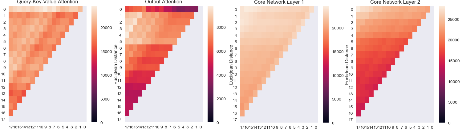
Figure 2: Euclidean Distance Between Trans-XL Weights: (1) Query-Key-Value Attention, (2) Output Attention, (3, 4) FC Layers

Language Modelling

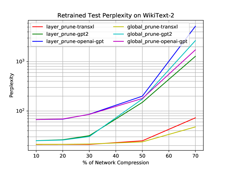
Figure 3: Wikitext-2 Language Modelling Pruning without Retraining

We begin by showing the similarity between pretrained layers on Transformer-XL in Figure 2, using sum of pairwise Euclidean distances. In general, we can see that closer layers have a smaller Euclidean distance. This more pronounced in the output attention (3) and fully connected layers (4) and slightly more sporadic among query-key-value attention weights (1).

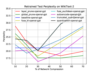
(a) GPT

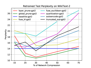
(b) GPT-2

(c) Transformer-XL

Figure 4: Language Modelling Compression Results on WikiText-2 with Retraining

In Figure 3, we find an exponential trend in perplexity (note the log-scale y-axis) increase with respect to the compression ratio for layer pruning and global pruning. Interestingly, Transformer-XL can maintain similar performance up to 50% pruning from the pretrained model without any retraining. In contrast, we see that the original OpenAI-GPT is more sensitive and begins to show an exponential increase at 30%. This insight is important for choosing the intervals between compress steps during iterative pruning, likewise for LF and tensor decomposition. Concretely, we would expect that the larger the increase in perplexity between compression steps, the more retraining epochs are needed. We also posit that this monotonically increasing trend in compression is related to the double descent phenomena (?), whereby when more data is added or the model complexity is reduced, the network can fall back into the critical regime region (?) and even further into the underparameterized regime. This is reinforced by the fact that a large network such as Transformer-XL contains a smaller global weight norm of fully-connected layers in comparison to GPT and is able to maintain similar performance up to 50% without retraining. Therefore, instead of choosing a constant $\%/N_{c}$ amount of compression at each compression step $N_{c}$, we allocate more compression earlier in retraining but more retraining steps later.

Figure 4 shows subfigures of retraining GPT (4(a)), GPT-2 (4(b)) and Transformer-XL (4(c)) with all aforementioned compression methods for GPT, GPT2 and Transformer-XL respectively. Firstly, we find retraining with a sufficient number of compression steps to be worthwhile for drastically reducing the network size while maintaining performance for both structured and unstructured approaches. Past 30% of network reduction wee find a weakly linear increase, in contrast to the exponential increase with no retraining. We find that global pruning generally outperforms layer pruning as it doesn’t restrict the percentage of weights pruned to be uniform across layers. This suggests that many layers are heavily pruned while others are preserved. This also coincides with findings from  (?) that some layers are critical to maintain performance while removing the remaining layers has little effect on generalization.

Table 3 shows the results of LF for compression ratio of 2 using layer averaging (Mean), layer freezing (Freeze) and mixing layers (-Mix) when ranking weight similarity using Euclidean distance (ED), KL and WS distance and CA. For all models CA produces the best results, slightly outperforming WS.

Table 3: WikiText-2 Perplexity after LF-Retraining (networks reduced to 50% their original size)

		Mean	Freeze	Mix
TransXL-KL		12.23	15.02	13.75
TransXL-ED		13.08	17.13	14.88
TransXL-WS		11.48	14.40	12.17
TransXL-CA		11.13	13.97	14.73
GPT2-KL		15.56	19.04	15.87
GPT2-ED		16.03	21.14	16.73
GPT2-WS		13.71	18.31	13.58
GPT2-CA		14.03	21.28	14.59
GPT-KL		23.57	28.01	24.82
GPT-ED		25.07	29.68	24.73
GPT-WS		19.10	23.17	18.90
GPT-CA		18.48	22.01	20.39

Additional Observations

In language modelling, the effects of model reduction typically follow an exponential increase in perplexity for a compression ratio greater than 2 (corresponding to @50%) when no retraining steps are used. Unlike CIFAR10 image classification, language modelling is a structured prediction task that has a relatively large output dimensionality which we posit has an important role in the amount of compression that can be achieved.  ? (?) have noted the softmax bottleck whereby the restriction on the size of the decoder results in information loss when calibrating the conditional distribution, while  (?) have also noted the double descent phenomena is dependent on the number of classes. We conjecture that pruning and other such methods can exacerbate this bottlenecking and therefore the compression ratio will be generally lower compared to classification problems with relatively less classes, such as CIFAR-10.

Conclusion

In this paper we proposed layer fusion, a new method for model compression. We find that merging the most similar layers during the retraining process of already deep pretrained neural network leads to competitive performance when compared against the original network, while maintaining a dense network. Layer fusion is also competitive with pruning, layer decomposition and knowledge distillation without the use of any additional parameters. We also find that mixing weight matrices during layer fusion performs comparably to layer averaging. Secondly, we compared how much compression can be achieved with and without retraining for both tasks and the importance of the number of epochs and compression steps. By using an exponential curriculum schedule to allocate the percentage of compression at each compression step, we find improvements over distributing the compression percentage uniformly during retraining. Lastly, a compression inflection point was observed in both tasks where the performance rapidly decreases, found for all compression methods and models.

References

- [Agustsson et al. 2017] Agustsson, E.; Mentzer, F.; Tschannen, M.; Cavigelli, L.; Timofte, R.; Benini, L.; and Gool, L. V. 2017. Soft-to-hard vector quantization for end-to-end learning compressible representations. In Advances in Neural Information Processing Systems, 1141–1151.
- [Argueta and Chiang 2019] Argueta, A., and Chiang, D. 2019. Accelerating sparse matrix operations in neural networks on graphics processing units. In Proceedings of the 57th Annual Meeting of the Association for Computational Linguistics, 6215–6224.
- [Ashok et al. 2017] Ashok, A.; Rhinehart, N.; Beainy, F.; and Kitani, K. M. 2017. N2n learning: Network to network compression via policy gradient reinforcement learning. arXiv preprint arXiv:1709.06030.
- [Ba, Kiros, and Hinton 2016] Ba, J. L.; Kiros, J. R.; and Hinton, G. E. 2016. Layer normalization. arXiv preprint arXiv:1607.06450.
- [Belkin et al. 2019] Belkin, M.; Hsu, D.; Ma, S.; and Mandal, S. 2019. Reconciling modern machine-learning practice and the classical bias–variance trade-off. Proceedings of the National Academy of Sciences 116(32):15849–15854.
- [Blumer et al. 1987] Blumer, A.; Ehrenfeucht, A.; Haussler, D.; and Warmuth, M. K. 1987. Occam’s razor. Information processing letters 24(6):377–380.
- [Dai et al. 2019] Dai, Z.; Yang, Z.; Yang, Y.; Cohen, W. W.; Carbonell, J.; Le, Q. V.; and Salakhutdinov, R. 2019. Transformer-xl: Attentive language models beyond a fixed-length context. arXiv preprint arXiv:1901.02860.
- [Dehghani et al. 2018] Dehghani, M.; Gouws, S.; Vinyals, O.; Uszkoreit, J.; and Kaiser, Ł. 2018. Universal transformers. arXiv preprint arXiv:1807.03819.
- [Devlin et al. 2018] Devlin, J.; Chang, M.-W.; Lee, K.; and Toutanova, K. 2018. Bert: Pre-training of deep bidirectional transformers for language understanding. arXiv preprint arXiv:1810.04805.
- [Fan, Grave, and Joulin 2019] Fan, A.; Grave, E.; and Joulin, A. 2019. Reducing transformer depth on demand with structured dropout. arXiv preprint arXiv:1909.11556.
- [Forrester and Kieburg 2016] Forrester, P. J., and Kieburg, M. 2016. Relating the bures measure to the cauchy two-matrix model. Communications in Mathematical Physics 342(1):151–187.
- [Frankle and Carbin 2018] Frankle, J., and Carbin, M. 2018. The lottery ticket hypothesis: Finding sparse, trainable neural networks. arXiv preprint arXiv:1803.03635.
- [Halko, Martinsson, and Tropp 2011] Halko, N.; Martinsson, P.-G.; and Tropp, J. A. 2011. Finding structure with randomness: Probabilistic algorithms for constructing approximate matrix decompositions. SIAM review 53(2):217–288.
- [Han et al. 2015] Han, S.; Pool, J.; Tran, J.; and Dally, W. 2015. Learning both weights and connections for efficient neural network. In Advances in neural information processing systems, 1135–1143.
- [Han, Mao, and Dally 2015] Han, S.; Mao, H.; and Dally, W. J. 2015. Deep compression: Compressing deep neural networks with pruning, trained quantization and huffman coding. arXiv preprint arXiv:1510.00149.
- [Hassibi and Stork 1993] Hassibi, B., and Stork, D. G. 1993. Second order derivatives for network pruning: Optimal brain surgeon. In Advances in neural information processing systems, 164–171.
- [He et al. 2016] He, K.; Zhang, X.; Ren, S.; and Sun, J. 2016. Deep residual learning for image recognition. In Proceedings of the IEEE conference on computer vision and pattern recognition, 770–778.
- [Hinton, Vinyals, and Dean 2015] Hinton, G.; Vinyals, O.; and Dean, J. 2015. Distilling the knowledge in a neural network. arXiv preprint arXiv:1503.02531.
- [Hochreiter and Schmidhuber 1997] Hochreiter, S., and Schmidhuber, J. 1997. Long short-term memory. Neural computation 9(8):1735–1780.
- [Huang et al. 2017] Huang, G.; Liu, Z.; Van Der Maaten, L.; and Weinberger, K. Q. 2017. Densely connected convolutional networks. In Proceedings of the IEEE conference on computer vision and pattern recognition, 4700–4708.
- [Iandola et al. 2014] Iandola, F.; Moskewicz, M.; Karayev, S.; Girshick, R.; Darrell, T.; and Keutzer, K. 2014. Densenet: Implementing efficient convnet descriptor pyramids. arXiv preprint arXiv:1404.1869.
- [Ioffe and Szegedy 2015] Ioffe, S., and Szegedy, C. 2015. Batch normalization: Accelerating deep network training by reducing internal covariate shift. arXiv preprint arXiv:1502.03167.
- [Karnin 1990] Karnin, E. D. 1990. A simple procedure for pruning back-propagation trained neural networks. IEEE transactions on neural networks 1(2):239–242.
- [Kornblith et al. 2019] Kornblith, S.; Norouzi, M.; Lee, H.; and Hinton, G. 2019. Similarity of neural network representations revisited. arXiv preprint arXiv:1905.00414.
- [Krizhevsky, Sutskever, and Hinton 2012] Krizhevsky, A.; Sutskever, I.; and Hinton, G. E. 2012. Imagenet classification with deep convolutional neural networks. In Advances in neural information processing systems, 1097–1105.
- [LeCun, Bengio, and others 1995] LeCun, Y.; Bengio, Y.; et al. 1995. Convolutional networks for images, speech, and time series. The handbook of brain theory and neural networks 3361(10):1995.
- [Lehmann 2004] Lehmann, E. L. 2004. Elements of large-sample theory. Springer Science & Business Media.
- [Li et al. 2016] Li, Y.; Yosinski, J.; Clune, J.; Lipson, H.; and Hopcroft, J. E. 2016. Convergent learning: Do different neural networks learn the same representations? In Iclr.
- [Long, Shelhamer, and Darrell 2015] Long, J.; Shelhamer, E.; and Darrell, T. 2015. Fully convolutional networks for semantic segmentation. In Proceedings of the IEEE conference on computer vision and pattern recognition, 3431–3440.
- [Merity et al. 2016] Merity, S.; Xiong, C.; Bradbury, J.; and Socher, R. 2016. Pointer sentinel mixture models. arXiv preprint arXiv:1609.07843.
- [Mishra and Marr 2017] Mishra, A., and Marr, D. 2017. Apprentice: Using knowledge distillation techniques to improve low-precision network accuracy. arXiv preprint arXiv:1711.05852.
- [Moakher and Batchelor 2006] Moakher, M., and Batchelor, P. G. 2006. Symmetric positive-definite matrices: From geometry to applications and visualization. In Visualization and Processing of Tensor Fields. Springer. 285–298.
- [Nakkiran et al. 2019] Nakkiran, P.; Kaplun, G.; Bansal, Y.; Yang, T.; Barak, B.; and Sutskever, I. 2019. Deep double descent: Where bigger models and more data hurt. arXiv preprint arXiv:1912.02292.
- [Orhan and Pitkow 2017] Orhan, A. E., and Pitkow, X. 2017. Skip connections eliminate singularities. arXiv preprint arXiv:1701.09175.
- [Polino, Pascanu, and Alistarh 2018] Polino, A.; Pascanu, R.; and Alistarh, D. 2018. Model compression via distillation and quantization. arXiv preprint arXiv:1802.05668.
- [Radford et al. 2018] Radford, A.; Narasimhan, K.; Salimans, T.; and Sutskever, I. 2018. Improving language understanding by generative pre-training. URL https://s3-us-west-2. amazonaws. com/openai-assets/researchcovers/languageunsupervised/language understanding paper. pdf.
- [Sanders and Kandrot 2010] Sanders, J., and Kandrot, E. 2010. CUDA by example: an introduction to general-purpose GPU programming, portable documents. Addison-Wesley Professional.
- [Shah et al. 2016] Shah, A.; Kadam, E.; Shah, H.; Shinde, S.; and Shingade, S. 2016. Deep residual networks with exponential linear unit. arXiv preprint arXiv:1604.04112.
- [Singh and Jaggi 2019] Singh, S. P., and Jaggi, M. 2019. Model fusion via optimal transport. arXiv preprint arXiv:1910.05653.
- [Strubell, Ganesh, and McCallum 2019] Strubell, E.; Ganesh, A.; and McCallum, A. 2019. Energy and policy considerations for deep learning in nlp. arXiv preprint arXiv:1906.02243.
- [Vaswani et al. 2017] Vaswani, A.; Shazeer, N.; Parmar, N.; Uszkoreit, J.; Jones, L.; Gomez, A. N.; Kaiser, Ł.; and Polosukhin, I. 2017. Attention is all you need. In Advances in Neural Information Processing Systems, 5998–6008.
- [Veit, Wilber, and Belongie 2016] Veit, A.; Wilber, M. J.; and Belongie, S. 2016. Residual networks behave like ensembles of relatively shallow networks. In Advances in neural information processing systems, 550–558.
- [Wu et al. 2016] Wu, J.; Leng, C.; Wang, Y.; Hu, Q.; and Cheng, J. 2016. Quantized convolutional neural networks for mobile devices. In Proceedings of the IEEE Conference on Computer Vision and Pattern Recognition, 4820–4828.
- [Yang et al. 2017] Yang, Z.; Dai, Z.; Salakhutdinov, R.; and Cohen, W. W. 2017. Breaking the softmax bottleneck: A high-rank rnn language model. arXiv preprint arXiv:1711.03953.
- [Yang et al. 2019] Yang, Z.; Dai, Z.; Yang, Y.; Carbonell, J.; Salakhutdinov, R.; and Le, Q. V. 2019. Xlnet: Generalized autoregressive pretraining for language understanding. arXiv preprint arXiv:1906.08237.
- [Zagoruyko and Komodakis 2016] Zagoruyko, S., and Komodakis, N. 2016. Wide residual networks. In BMVC.
- [Zhang, Bengio, and Singer 2019] Zhang, C.; Bengio, S.; and Singer, Y. 2019. Are all layers created equal? arXiv preprint arXiv:1902.01996.