Neutrinoless Double-Electron Capture

Abstract

Double-beta processes play a key role in the exploration of neutrino and weak interaction properties, and in the searches for effects beyond the Standard Model. During the last half century many attempts were undertaken to search for double-beta decay with emission of two electrons, especially for its neutrinoless mode ($0\nu 2\beta^{-}$), the latter being still not observed. Double-electron capture (2EC) was not in focus so far because of its in general lower transition probability. However, the rate of neutrinoless double-electron capture ($0\nu 2$EC) can experience a resonance enhancement by many orders of magnitude in case the initial and final states are energetically degenerate. In the resonant case, the sensitivity of the $0\nu 2$EC process can approach the sensitivity of the $0\nu 2\beta^{-}$ decay in the search for the Majorana mass of neutrinos, right-handed currents, and other new physics. We present an overview of the main experimental and theoretical results obtained during the last decade in this field. The experimental part outlines search results of 2EC processes and measurements of the decay energies for possible resonant $0\nu$2EC transitions. An unprecedented precision in the determination of decay energies with Penning traps has allowed one to refine the values of the degeneracy parameter for all previously known near-resonant decays and has reduced the rather large uncertainties in the estimate of the $0\nu 2$EC half-lives. The theoretical part contains an updated analysis of the electron shell effects and an overview of the nuclear structure models, in which the nuclear matrix elements of the $0\nu 2$EC decays are calculated. One can conclude that the decay probability of $0\nu$2EC can experience a significant enhancement in several nuclides.

I Introduction

In 1937, Ettore Majorana found an evolution equation for a truly neutral spin-1/2 fermion Majorana (1937). His work was motivated by the experimental observation of a free neutron by James Chadwick in 1932. Majorana also conjectured that his equation applies to a hypothetical neutrino introduced by Wofgang Pauli to explain the continuous spectrum of electrons in the $\beta$ decay of nuclei. In the mid-1950s, Reines and Cowan (1956, 1959) discovered a particle with neutrino properties. At the time of the establishment of the Standard Model (SM) of electroweak interactions, three families of neutrinos were known. While the neutron is a composite fermion consisting of quarks, neutrinos acquired the status of elementary particles with zero masses in the SM framework. The discovery of neutrino oscillations by the Super-Kamiokande collaboration Fukuda et al. (1998) showed that neutrinos are mixed and massive. A comprehensive description of the current state of neutrino physics can be found in the monograph of Bilenky (2018).

Whether neutrinos are truly neutral fermions is one of the fundamental questions in modern particle physics, astrophysics and cosmology. The fermions described by the Dirac equation can also be electrically neutral. However, even in this case, there is a conserved current in Dirac s theory, which ensures a constant number of particles (minus antiparticles). Majorana fermions, like photons, do not have such a conserved current. In Dirac’s theory, particles and antiparticles are independent, while Majorana fermions are their own antiparticles and, via CPT, it follows that they must have zero charge. Truly neutral spin-1/2 fermions are referred to as Majorana fermions and those with a conserved current are referred to as Dirac fermions. Majorana fermions in bispinor basis are vectors of the real vector space $\mathbb{R}^{4}$. They can also be described by two-component Weyl spinors in the complex space $\mathbb{C}^{2}$. In both representations, the superposition principle for Majorana fermions holds over the field of real numbers. Majorana fermions belong to the fundamental real representation of the Poincaré group. A Dirac fermion of mass $m$ can be represented as a superposition of two Majorana fermions of masses $m$ and $-m$, respectively.

The neutron has a non-vanishing magnetic moment, so it cannot be a pure Majorana particle. On the other hand, there is no fundamental reason to claim that it is a pure Dirac particle. In theories with nonconservation of the baryon number, the mass eigenstates include a mixture of baryons and antibaryons. At the phenomenological level, the effect is modeled by adding a Majoranian mass term to the effective Lagrangian. As a result, the neutron experiences oscillations $n\leftrightarrow\bar{n}$, whereby the nuclei decay with nonconservation of the baryon number Dover et al. (1983, 1985); Krivoruchenko (1996a, b); Gal (2000); Kopeliovich and Potashnikova (2010); Phillips et al. (2016). Experimental limits for the period of the $n\leftrightarrow\bar{n}$ oscillations in the vacuum, $\tau_{\mathrm{vac}}>2.7\times 10^{8}$ s Abe et al. (2015), constrain the neutron Majorana mass to $\Delta m\sim 1/\tau_{\mathrm{vac}}<0.8\times 10^{-33}m$, where $m=939.57$ MeV/c² is the neutron Dirac mass. Thus, under the condition of nonconservation of the baryon number, Majorana’s idea on the existence of truly neutral fermions can be partially realized in relation to the neutron. In contrast, neutrinos can be pure Majorana fermions or pure Dirac fermions, or a mixture of these two extreme cases. It is noteworthy that none of the variants of neutrino masses are possible within the SM. The neutrino mass problem leads us to physics beyond the SM. Alternative examples of Majorana particles include weakly interacting dark matter candidates and Majorana zero modes in solid state systems Elliott and Franz (2015).

Searches for neutrinoless double-beta ($0\nu 2\beta^{-}$) decay, neutrinoless double-electron capture ($0\nu$2EC) by nuclei and other lepton number violating (LNV) processes provide the possibility to shed light on the question of the nature of neutrinos: whether they are Majorana or Dirac particles. By virtue of the black-box theorem Hirsch et al. (2006); Schechter and Valle (1982), the observation of the $0\nu 2\beta$ decay would prove that neutrinos have a finite Majorana mass. The massive Majorana neutrinos lead to a violation of the conservation of the total lepton number $L$. In the quark sector of SM, the baryon charge, $B$, is a similar quantum number. Vector currents of $B$ and $L$ are classically conserved. Left handed fermions are associated with the $SU(2)$ electroweak gauge fields $W^{\pm}$ and $Z^{0}$, so that vector currents of $B$ and $L$, as ’t Hooft first pointed out ’t Hooft (1976), are sensitive to the axial anomaly. Through electroweak instantons, this leads to nonconservation of $B$ and $L$, while the difference $(B-L)$ is conserved. The violating amplitude is exponentially suppressed. Another example is given by sphaleron solutions of classical field equations of SM, that preserve $(B+L)$ but violate $B$ and $L$ individually, which can be relevant for cosmological implications White (2016). The conservation of $(B-L)$ within SM is not supported by any fundamental principle analogous to local gauge symmetry, so $B$ and $L$ can be broken beyond SM explicitly. Experimental observation of the proton decay and/or $n\leftrightarrow\bar{n}$ oscillations could prove nonconservation of $B$, while observation of the $0\nu 2\beta^{-}$ decay and/or the $0\nu$2EC process could prove nonconservation of $L$ with constant $B$. Moreover, these processes are of interest for determining the absolute neutrino mass scale, the type of neutrino mass hierarchy, and the character of CP violation in lepton sector. Due to the exceptional value of LNV processes, vast literature is devoted to physics of $0\nu 2\beta^{-}$ decay and the underlined nuclear structure models (for reviews see Vergados et al. (2012); Raduta (2015); Engel and Menéndez (2017); Ejiri et al. (2019); Suhonen (2007); Bilenky and Petcov (1987); Zdesenko (2002); Avignone III et al. (2008)).

The $0\nu 2\beta^{-}$ decay was first discussed by Furry (1939). The process is shown in Fig. 1. A nucleus with the mass number $A$ and charge $Z$ experiences $0\nu 2\beta^{-}$ decay accompanied by the exchange of a Majorana neutrino between the nucleons:

$$(A,Z)\to(A,Z+2)^{++}+e^{-}+e^{-},$$ (I.1)

where $(A,Z+2)^{++}$ is the doubly ionized atom in the final state. There are many models beyond SM that provide alternative mechanisms of the $0\nu 2\beta^{-}$-decay, some of which are discussed in Sec. II.

In 1955, the related $0\nu 2$EC process

$$e^{-}_{b}+e^{-}_{b}+(A,Z)\to(A,Z-2)^{**}$$ (I.2)

was discussed by Winter Winter (1955a). Here $e^{-}_{b}$ are bound electrons. The nucleus and the electron shell of the neutral atom $(A,Z-2)^{**}$ are in excited states. An example of the mechanism related to the Majorana neutrino exchange is shown in Fig. 2. Subsequent de-excitation of the nucleus occurs via gamma-ray radiation or $\beta$ decays. De-excitation of the electron shell is associated with the emission of Auger electrons or gamma rays in a cascade formed by filling of electron vacancies. In the absence of special selection rules, dipole radiation dominates in X-rays. Since the dipole moment of electrons is much higher than that of nucleons in the nucleus, the de-excitation of the electron shell goes faster. For atoms with a low value of $Z$, the Auger electron emission is more likely. With increase in the atomic number, the radiation of X-ray photons becomes dominant. The de-excitation of high electron orbits is due to Auger-electron emission for all $Z$.

Estimates show that the sensitivity of the $0\nu 2$EC process to the Majorana neutrino mass is many orders of magnitude lower than that of the $0\nu 2\beta^{-}$ decay. Winter pointed out that degeneracy of the energies of the parent atom $(A,Z)$ and the daughter atom $(A,Z-2)^{**}$ gives rise to resonant enhancement of the decay. In the early 80s, a number of other authors also remarked on the possible resonant enhancement of the $0\nu 2$EC process Georgi et al. (1981); Voloshin et al. (1982). The resonances in 2EC were considered, however, as an unlikely coincidence.

Figure 1: Schematic representation of neutrinoless double-beta decay: Two neutrons in the nucleus experience $\beta$ decay accompanied by the exchange of a Majorana neutrino. Neutrons, protons, electrons and neutrinos are represented by solid lines. Arrows show the flow of baryon charge of protons and neutrons and the flow of lepton charge of electrons and neutrinos. The cross denotes the Majorana neutrino mass term, $m_{L}$, that causes the helicity-flip of the intermediate neutrino and violates lepton number by two units.

To compensate for the low probability of the $0\nu$2EC process by a resonance effect, it is necessary to determine the energy difference of atoms with high accuracy. The decay probability is proportional to the Breit-Wigner factor $\Gamma_{f}/(\Delta^{2}+\Gamma_{f}^{2}/4)$, where $\Gamma_{f}$ is the electromagnetic decay width of the daughter atom and $\Delta=M_{A,Z}-M^{**}_{A,Z-2}$ is the degeneracy parameter equal to the mass difference of the parent and the daughter atoms. The maximum increase in probability is achieved for $\Delta=0$ when the decay amplitude approaches the unitary limit. Taking $\Delta\sim 10$ keV for the typical splitting of the masses of the atoms and $\Gamma_{f}\sim 10$ eV for the typical decay width of the excited electron shell of the daughter atom, one finds the maximum enhancement of $\sim 10^{6}$. The degeneracy parameter $\Delta\lesssim\Gamma_{f}$ gives the half-life of a nuclide with respect to $0\nu$2EC comparable to the half-life of nuclides with respect to $0\nu 2\beta^{-}$ decay.

The near-resonant $0\nu 2$EC process was analyzed in detail by Bernabeu et al. (1983). The authors developed a non-relativistic formalism of the resonant $0\nu 2$EC in atoms and specified a dozen of nuclide pairs for which degeneracy is not excluded. The $0\nu 2$EC process became the subject of a detailed theoretical study by Sujkowski and Wycech (2004). A list of the near-resonant $0\nu 2$EC nuclide pairs is also provided by Karpeshin (2008). The problem acquired an experimental character: the difference between masses of the parent and daughter atoms, i.e. $Q$-values, known to an accuracy of about 10 keV, which is too far from the accuracy required to identify the unitary limit. The determination of the degeneracy parameter has acquired fundamental importance.

In the 1980s, there was no well-developed technique to measure the masses of nuclides with relative uncertainty of about $10^{-9}$ sufficient to find resonantly enhanced $0\nu 2$EC processes. The presently state-of-the-art technique high-precision Penning-trap mass spectrometry was still in its infancy. Its triumphal advance in the field of high-precision mass measurements on radioactive nuclides began with the installation of the ISOLTRAP facility at CERN in the late 1980s Bollen et al. (1987); Mukherjee et al. (2008); Kluge (2013). The last decades was marked by a rising variety of high-precision Penning-trap facilities in Europe, the USA and Canada Blaum (2006); Blaum et al. (2013). This lead to a tremendous development of Penning-trap mass-measurement techniques Kretzschmar (2007); George et al. (2007a); Eliseev et al. (2007); Kretzschmar (2013); Blaum et al. (2013); Eliseev et al. (2013, 2014) and finally made it possible to routinely carry out mass measurements on a broad variety of nuclides with a relative uncertainty of about 10^-9. The mass of the ion is determined via the measurement of its free cyclotron frequency in a pure magnetic field, the most precisely measurable quantity in physics.

These factors motivated a new study of the near-resonant $0\nu 2$EC process. A relativistic formalism for calculating electron shell effects was developed and an updated realistic list of nuclide pairs for which the measurement of $Q_{\mathrm{2EC}}$ values ​ ​has high priority was compiled Krivoruchenko et al. (2011). Also a significantly refreshed database of the nuclides and their excited states is now available, thirty years since the previous publication by Bernabeu et al. (1983). An overview of the investigation of the resonant $0\nu$2EC is given by Eliseev et al. (2012) including the persistent experimental attempts to search for appropriate candidates for this extraordinary phenomenon.

Figure 2: Schematic representation of neutrinoless double-electron capture: Two protons in the nucleus each capture a bound electron from the electron shell and turn into two neutrons by the exchange of a Majorana neutrino. Notations are the same as in Fig. 1.

The advancements of the experiments in search of the $0\nu$2EC process are lower than of those searching for $0\nu 2\beta^{-}$ decay. While the sensitivity of the $0\nu 2\beta^{-}$ experiments approaches half-life limits $T_{1/2}\sim 10^{24}-10^{26}$ yr, which constrains the effective Majorana neutrino mass of electron neutrino to $|m_{\beta\beta}|\lesssim 0.1-0.7$ eV, the results of the best $0\nu$2EC experiments are yet on the level of $T_{1/2}\sim 10^{19}-10^{22}$ yr. The reasons for this difference are rather obvious: there is usually a much lower relative abundance of the isotopes of interest (typically lower than 1%), and additionally a more complicated effect signature due to the emission of a gamma-quanta cascade (instead of a clear $0\nu 2\beta^{-}$ peak at the decay energy). The second circumstance results in a lower detection efficiency for the most energetic peak in a $0\nu$2EC energy spectrum. Furthermore, the energy of the most energetic $0\nu$2EC peak is generally lower than in the $0\nu 2\beta^{-}$ processes, yet the higher the energy of a certain process the better the suppression of the radioactive background. As a result the scale of the 2EC experiments is substantially smaller than that of the $0\nu 2\beta^{-}$ ones. At the same time, there is a motivation to search for the neutrinoless EC$\beta^{+}$ and $2\beta^{+}$ decays owing to the potential to clarify the possible contribution of the right-handed currents to the $0\nu 2\beta^{-}$ decay rate Hirsch et al. (1994), and the appealing possibility of the resonant $0\nu$2EC processes. The complicated effect signature expected in resonant $0\nu$2EC transitions becomes an advantage: the detection of several gamma quanta with well-known energies could be a strong proof of the pursued effect.

The above mentioned aspects of the phase space, degeneracy, abundance factors, etc. play an important role in determining the half-lives of the $0\nu$EC$\beta^{+}$ and $0\nu$2EC processes. A further ingredient affecting the decay half-lives are the involved nuclear matrix elements (NMEs), see the reviews Maalampi and Suhonen (2013); Suhonen (2012a); Ejiri et al. (2019). These NMEs have been calculated in various nuclear-theory frameworks for a number of nuclei. In this review we use these NMEs, as well as NMEs which have been calculated just for this review, to estimate the half-lives of those $0\nu$2EC transitions which are of interest due to their (possibly) favorable resonance conditions.

II Double-electron capture and physics beyond the Standard Model

The underlying quark-level physics behind the $0\nu$2EC process (see Eq. (I.2)) is basically the same as for the $0\nu 2\beta^{-}$, $0\nu 2\beta^{+}$ and $0\nu$EC$\beta^{+}$ decays. In Figs. 1 and 2, we show the mechanism of exchange of light or heavy Majorana neutrinos that arises beyond the Standard Model within the Weinberg effective Lagrangian approach Weinberg (1979). In the Weinberg scenario, the Majorana mass occurs from LNV operator of dimension 5, which provides conditions for the existence of the processes $0\nu$2EC and $0\nu 2\beta^{-}$. A violation of the lepton number can also occur from quark-lepton effective Lagrangians of higher dimensions, corresponding to other possible mechanisms of the $0\nu 2$EC process. The neutrinoless 2EC can be accompanied by the emission of one or more very light particles, other than neutrinos in $2\nu$2EC. A well-known example is the Majoron, $J$, as the Goldstone boson of a spontaneously broken $U(1)_{L}$-symmetry of lepton number. Passing to the hadronic level one meets two possibilities of hadronization of the quark-level underlying process, known from $0\nu 2\beta^{-}$ decay: direct nucleon and pionic mechanisms. Below we consider the above-mentioned aspects of the $0\nu$2EC process in more detail.

First of all, the underlying quark level mechanisms of the neutrinoless 2EC can be classified according to the possible exotic final states:

$\bullet$ No exotic particles in the final state: the reaction $0\nu$2EC is shown in Eq. (I.2).

$\bullet$ The reaction $0\nu$2EC$nJ$: $e^{-}_{b}+e^{-}_{b}+(A,Z)\to(A,Z-2)^{**}+nJ,$ with $n$ being the number of Majorons or Majoron-like exotic particles in the final state.

Both kinds of reaction can be further classified by the typical distance between particles involved in the underlying quark-lepton process, depending on the masses of the intermediate particles Päs et al. (1999, 2001); Prezeau et al. (2003); Cirigliano et al. (2018b, a), as illustrated in Fig. 3.

$\bullet$ Long-range mechanisms with the Weinberg $d=5$ operator of Fig. 3 (a) and an effective $d=6$ operator in the upper vertex of Fig. 3 (b).

$\bullet$ Short-range mechanisms with a dimension 9 effective operator in the vertex of Fig. 3 (c).

The effective operators in the low-energy limit originate from diagrams with heavy exotic particles in the internal lines.

The diagrams of the $0\nu$2EC$nJ$ decays are derived from those in Fig. 3 by inserting one or more scalar Majoron lines either into the blobs of effective operators or into the central neutrino line of Fig. 3 (a).

II.1 Quark-level mechanisms of $0\nu$2EC

Let us consider in more detail the short- and long-ranged mechanisms of $0\nu 2$EC. The corresponding diagrams for the $0\nu 2$EC process are shown in Fig. 3. The blobs in Figs. 3 (b,c) represent the $\Delta L=2$ effective vertices beyond the SM. At the low-energy scales $\mu\sim 100$ MeV, typical for $0\nu 2$EC process, the blobs are essentially point-like, being generated by the exchange of a heavy particle with the characteristic masses $M_{H}$ much larger than the $0\nu 2$EC-scale, i.e. $M_{H}\gg\mu$. Integrating them out one finds the effective Lagrangian terms describing the vertices at the scale $\mu\ll\Lambda\sim M_{H}$ for any kind of underlying high-scale physics beyond SM. These vertices can be written in the following form Päs et al. (1999, 2001)

$$\mathcal{L}_{ql}^{(6)} = \frac{G_{F}}{\sqrt{2}}\left(-j_{CC}^{\mu}J_{CC\,\mu}+\sum_{i}C^{X}_{i}(\mu)\mathcal{O}^{(6)X}_{i}(\mu)\right),$$ (II.1)

$${\cal L}^{(9)}_{ql} = \frac{G_{F}^{2}}{2m_{p}}\,\sum_{i,XY}C_{i}^{XY}(\mu)\cdot\mathcal{O}^{(9)XY}_{i}(\mu).$$ (II.2)

The first and second lines correspond to Figs. 3 (b) and (c), respectively. The proton mass $m_{p}$ is introduced to match the conventional notations. The complete set of the $\Delta L=2$ operators for $d=6$ and $9$ is as follows González et al. (2016); Arbeláez et al. (2016, 2017):

$$\mathcal{O}_{1}^{(6)X} = 4(\bar{d}P_{X}u)\left(\overline{\nu^{c}}P_{L}e\right),$$ (II.3)

$$\mathcal{O}_{2}^{(6)X} = 4(\bar{d}\sigma^{\mu\nu}P_{X}u)\left(\overline{\nu^{c}}\sigma^{\mu\nu}P_{L}e\right)$$ (II.4)

$$\mathcal{O}_{3}^{(6)X} = 4(\bar{d}\gamma_{\mu}P_{X}u)\left(\overline{\nu^{c}}\gamma^{\mu}P_{R}e\right).$$ (II.5)

$$\mathcal{O}^{(9)XY}_{1} = 4({\bar{d}}P_{X}u)({\bar{d}}P_{Y}u)\ j,$$ (II.6)

$$\mathcal{O}^{(9)XY}_{2} = 4({\bar{d}}\sigma^{\mu\nu}P_{X}u)({\bar{d}}\sigma_{\mu\nu}P_{X}u)\ j,$$ (II.7)

$$\mathcal{O}^{(9)XY}_{3} = 4({\bar{d}}\gamma^{\mu}P_{X}u)({\bar{d}}\gamma_{\mu}P_{Y}u)\ j,$$ (II.8)

$$\mathcal{O}^{(9)XY}_{4} = 4({\bar{d}}\gamma^{\mu}P_{X}u)({\bar{u}}\sigma_{\mu\nu}P_{Y}d)\ j^{\nu},$$ (II.9)

$$\mathcal{O}^{(9)XY}_{5} = 4({\bar{d}}\gamma^{\mu}P_{X}u)({\bar{d}}P_{Y}u)\ j_{\mu},$$ (II.10)

where $X,Y=L,R$ and the leptonic currents are $j=\overline{e^{c}}(1\pm\gamma_{5})e$, $j_{\mu}=\overline{e^{c}}\gamma_{\mu}\gamma_{5}e.$ The first term in Eq. (II.1) describes the SM low-energy 4-fermion effective interaction of the Charged Current (CC):

$$j_{CC}^{\mu}=\bar{\nu}\gamma^{\mu}(1-\gamma_{5})e,\ \ \ J_{CC\,\mu}=\bar{d}\gamma_{\mu}(1-\gamma_{5})u.$$ (II.11)

The $SU(3)_{c}\times U(1)_{em}$-symmetric operators in Eqs. (II.3) - (II.10) are written in the mass-eigenstate basis. They originate from the $SU(3)_{c}\times SU(2)_{W}\times U(1)_{Y}$ gauge invariant operators after the electroweak symmetry breaking (see, e.g., the papers of Bonnet et al. (2013); Lehman (2014); Graesser (2017)).

The diagrams in Figs. 3 (a,b) are of second-order in the Lagrangian (II.1). The effect of $\Delta L=2$ is introduced in the diagrams (a) and (b) by the Majorana neutrino mass term and by the $d=6$ effective operators (II.3) - (II.5), respectively. The diagram in Fig. 3 (a) is the conventional Majorana neutrino mass mechanism with the contribution to the $0\nu 2$EC amplitude

$$V_{\alpha\beta} \sim m_{\beta\beta}\equiv\sum_{i}U^{2}_{ei}m_{\nu_{i}},$$ (II.12)

where $U$ is the Pontecorvo - Maki - Nakagawa - Sakata (PMNS) mixing matrix and $m_{\beta\beta}$ is the effective electron neutrino Majorana mass parameter well-known from the analysis of $0\nu 2\beta^{-}$ decay. The contribution of the diagram of Fig. 3 (b) is independent of the neutrino mass, but proportional to the momentum $q$ flowing in the neutrino propagator. This is the so-called $\hat{q}$-type contribution.

The following comment is in order. The diagrams in Fig. 3 (a,b) show two possible mechanisms of both $0\nu 2$EC and $0\nu 2\beta^{-}$ (with the inverted final to initial states) processes. The first mechanism Fig. 3 (a) contributes to the amplitude of these processes with terms proportional to the effective Majorana mass parameter $m_{\beta\beta}$ defined in (II.12). The contribution of the second mechanism Fig. 3 (b) has no explicit dependence on $m_{\beta\beta}$. This is because the upper vertex in Fig. 3 (b) breaks lepton number in two units as necessary for this process to proceed without the need of the $\Delta L=2$ Majorana neutrino mass insertion into the neutrino line. Note that $m_{\beta\beta}=0$ is compatible with the neutrino oscillation data in the case of Normal neutrino mass Ordering. This result shows that the mechanism Fig. 3 (a), proportional to $m_{\beta\beta}$, can be negligible in comparison with the mechanism in Fig. 3 (b). Therefore, even if $m_{\beta\beta}$ turns out to be very small, both $0\nu 2\beta^{-}$ decay and $0\nu 2$EC process can be observable due to the latter mechanism. This possibility has been studied in the literature for $0\nu 2\beta^{-}$ decay (see, e.g., the papers of Päs et al. (1999, 2001); Arbeláez et al. (2016, 2017); González et al. (2016)).

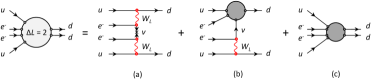
Figure 3: A decomposition of the generic $\Delta L=2$ vertex into the long-range (a), (b) and the short-range (c) quark-level contributions to $0\nu 2$EC. The diagram (a) is the conventional Majorana neutrino mass mechanism. The blobs in (b) and (c) denote the effective $\Delta L=2$ vertices.

The SM gauge invariant Weinberg dimension-5 effective operator generating the neutrino mass mechanism is given by Weinberg (1979)

$$\mathcal{L}^{(5)}_{W} = \kappa\frac{\left(\overline{L^{c}}\cdot H\right)\left(L\cdot H\right)}{\Lambda}=\frac{\kappa}{\Lambda}\overline{\nu^{c}}\nu H^{0}H^{0}+...$$ (II.13)

$$\xrightarrow[]{SSB} \kappa\frac{\langle H^{0}\rangle^{2}}{\Lambda}\overline{\nu^{c}}\nu+...\;.$$

In the above equation we mean $L\cdot H=L_{i}H_{j}\epsilon_{ij}$ the singlet combination of two $SU(2)_{W}$ doublets $L(\overline{L^{c}})$ and $H$.After the electroweak spontaneous symmetry breaking (SSB) with the Higgs vacuum expectation value $\langle H\rangle\neq 0$ neutrinos acquire a Majorana mass $m_{\nu}=-2\kappa\langle H\rangle^{2}/\Lambda$, with $\kappa$ being a dimensionless parameter. In the flavor basis of neutrino states the contribution of the Weinberg operator to an LNV process such as $0\nu 2$EC is displayed in Fig. 4. The summation of multiple insertions of the Weinberg operator into the bare neutrino propagator entails the renormalized neutrino propagator with Majorana mass $m_{\nu}$. The operator (II.13) is unique. Other operators of the effective Lagrangian are suppressed by higher powers of the unification scale $\Lambda$. The study of the neutrinoless 2EC process and $2\beta^{-}$ decays could be the most direct way of testing physics beyond the Standard Model. In terms of the naive dimensional counting one can expect the dominance of the Weinberg operator, with the dimension 5, over the operators of dimensions 6 and 9 in Eqs. (II.5) - (II.6). However, in order to set $m_{\nu}$ at eV-scale one should provide a very small coupling $\kappa\sim 10^{-11}$ for the phenomenologically interesting case of $\Lambda\sim O$(1 TeV). However, the smallness of any dimensionless coupling requires explanation. Typically in this case one expects the presence of some underlying physics, for example, symmetry. The situation changes with the increase of the LNV scale up to $\Lambda\sim 10^{13-14}$, with $\kappa\sim 1$, where the contribution of the Weinberg operator to $0\nu 2$EC dominates. The final count depends on the concrete high-scale underlying LNV model: not all operators appear in the low-energy limit and $\kappa$ is a small suppression factor allowing TeV-scale $\Lambda$. The latter can stem from loops or the ratio of the SSB scales in multi-scale models (for a recent analysis see, e.g., the paper of Helo et al. (2016)).

In this review the mechanism of the neutrino Majorana masses is discussed in detail, for which numerical evaluation of the neutrinoless 2EC half-lives of near-resonant nuclides with the known NMEs will be given. In the case of high-dimensional operators, as well as for the d = 5 mechanism with the unknown NMEs, normalized estimates will be given, which take into account the factorization of nuclear effects in the $0\nu$2EC amplitude. Keeping the above comments in mind, we also discuss mechanisms based on the operators of Eqs. (II.5) - (II.6), leading to the contributions shown in Figs. 3 (b,c).

The blobs in the diagrams of Figs. 3 (b,c) can be opened up (ultraviolet completed) in terms of all possible types of renormalizable interactions consistent with the SM gauge invariance. These are the high-scale models, which lead to the $0\nu 2$EC process. A list of all the possible ultraviolet completions for $0\nu 2\beta^{-}$ decay is given by Bonnet et al. (2013).

The Wilson coefficients $C_{i}$ in Eqs. (II.1), (II.2) are calculable in terms of the parameters (couplings and masses) of a particular underlying model at the scale $\Lambda\sim M_{H}$, called “matching scale”. Note that some of $C_{i}(\Lambda)$ may vanish. In order to make contact with $0\nu 2$EC one needs to estimate $C_{i}$ at a scale $\mu_{0}$ close to the typical $0\nu 2$EC-energy scale. The coefficients $C_{i}$ run from the scale $\Lambda$ down to $\mu_{0}$ due to the QCD corrections. Also the $d=9$ operators undergo the RGE-mixing with each other leading to the mixing of the corresponding Wilson coefficients.

The general parameterization of the $0\nu 2$EC amplitude derived from the diagrams in Fig. 3, taking into account the leading order QCD-running González et al. (2016); Cirigliano et al. (2018a); Liao et al. (2020); Ayala et al. (2020), reads:

$$V_{\alpha\beta}=G_{F}^{2}\cos^{2}\theta_{C}K_{Z}\left(\sum_{i=1}^{3}\beta_{i}^{X}(\mu_{0},\Lambda)C_{i}^{X}(\Lambda)\right.+\left.\sum_{i=1}^{5}\beta_{i}^{XY}(\mu_{0},\Lambda)C_{i}^{XY}(\Lambda)\right)\mathcal{A}_{\alpha\beta}.$$ (II.14)

The parameters $\beta_{i}^{X}$ and $\beta_{i}^{XY}$ incorporate the QCD-running of the Wilson coefficients and the matrix elements of the operators in Eqs.(II.3) - (II.5) combined with $j_{CC}^{\mu}J_{CC\,\mu}$ and the operators in Eqs. (II.6) - (II.10). The wave functions of the captured electrons with quantum numbers $\alpha$ and $\beta$ enter the coefficients $\mathcal{A}_{\alpha\beta}$ defined by Eqs. (IV.20) - (IV.23). In Eq. (II.14) the summation over the different chiralities $X,Y=L,R$ is implied. It is important to note that the Wilson coefficients $C_{i}(\Lambda)$ entering Eqs. (II.1) and (II.2) are linked to the matching scale $\Lambda$, where they are calculable in terms of the Lagrangian parameters of a particular high-scale underlying model. The decay amplitude (II.14) is supplemented by the overlap amplitude $K_{Z}$ of the electron shells of the initial and final atoms. In this review, we discuss mainly the light Majorana neutrino exchange mechanism of Fig. 3 (a).

The $0\nu 2$EC NMEs are currently known only for the Majorana neutrino exchange mechanisms coupled to left- and right-handed currents. Calculations of the NMEs corresponding to the other long- and short-range mechanisms of Figs. 3 (b) and (c), respectively, for all operators (II.5) - (II.6) are still in progress.

Figure 4: The contribution of the Weinberg operator to the $0\nu 2$EC process in the flavor basis of the neutrino states.

II.2 Examples of underlying high-scale models

We give three examples of popular high-scale models that can underlie the $0\nu 2$EC process. In the low-energy limit their contribution is described by the effective Lagrangians (II.1) and/or (II.2).

$\bullet$ Left-Right symmetric models: A well-known example of a high-scale model leading to $\Delta L=2$ processes, such as $0\nu 2\beta$-decay and $0\nu 2$EC as well as generating Majorana mass for neutrinos, is the Left-Right symmetric extension of the SM. The Left-Right Symmetric Model (LRSM) is based on the gauge group $\mathcal{G}$ spontaneously broken via the chain

$$\mathcal{G}=SU(3)_{C}\times SU(2)_{L}\times SU(2)_{R}\times U(1)_{B-L}$$ (II.15)

$$\Downarrow\ \ v_{R}$$

$$SU(3)_{C}\times SU(2)_{L}\times U(1)_{Y}$$

$$\ \ \Downarrow\ \ v_{SM}$$

$$SU(3)_{C}\times U(1)_{em}.$$

where $v_{R}\equiv\langle\Delta_{R}\rangle\gg\langle\Phi\rangle\equiv v_{SM}$ are the vacuum expectation values (VEV) of a Higgs $SU(2)_{R}$-triplet, $\Delta_{R}$ and a Higgs bi-doublet, $\Phi$, respectively. The bi-doublet belongs to the doublet representation of both $SU(2)_{L}$ and $SU(2)_{R}$. There is also a Higgs $SU(2)_{L}$-triplet, $\Delta_{L}$, with the VEV $v_{L}\equiv\langle\Delta_{L}\rangle$. Left- and right-handed leptons and quarks belong to the doublet representations of the $SU(2)_{L}$ and $SU(2)_{R}$ gauge groups, respectively. The $SU(3)_{C}\times SU(2)_{L}\times SU(2)_{R}\times U(1)_{B-L}$ assignments of the LRSM fields are

$$L_{{L(R)}} = \left(\begin{array}[]{c}\nu_{i}\\ \ell^{-}_{i}\end{array}\right)_{L(R)}\sim\left[1,2(1),1(2);-1\right],$$ (II.18)

$$Q_{L(R)} = \left(\begin{array}[]{c}u_{i}\\ d_{i}\end{array}\right)_{L(R)}\sim\left[3,2(1),2(1);-1/3\right],$$ (II.21)

$$\Delta_{L(R)} = \left(\begin{array}[]{cc}\frac{\Delta^{+}}{\sqrt{2}}&\Delta^{++}\\ \Delta^{0}&\frac{-\Delta^{+}}{\sqrt{2}}\end{array}\right)_{L(R)}\sim\left[1,3(1),1(3);2\right],$$ (II.24)

$$\Phi = \left(\begin{array}[]{cc}\Phi_{1}^{0}&\Phi_{1}^{+}\\ \Phi_{2}^{-}&\Phi_{2}^{0}\end{array}\right)\sim\left[1,2,2;0\right],$$ (II.27)

where $i=1,2,3$ is the generation index. Previously introduced VEVs are related with the VEVs of the electrically neutral components $\langle\Delta_{L,R}\rangle\equiv\langle\Delta_{L,R}^{0}\rangle$, $\langle\Phi\rangle^{2}=\langle\Phi^{0}_{1}\rangle^{2}+\langle\Phi^{0}_{2}\rangle^{2}\equiv v_{SM}$. There are two charged gauge bosons $W^{\pm}_{L,R}$ and two neutral gauge bosons $Z_{L,R}$ with masses of the order $M_{W_{R}},M_{Z_{R}}\sim g_{R}v_{R}$, $M_{W_{L}},M_{Z_{L}}\sim g_{L}v_{SM}$. Note that in the scenario with the manifest Left-Right symmetry the $SU(2)_{L,R}$-gauge couplings obey $g_{L}=g_{R}$. Since the bosons $W_{R},Z_{R}$ have not been experimentally observed, the scale of the left-right symmetry breaking $v_{R}$ must be sufficiently large, above few TeV. On the other hand the VEV of the “left” triplet $v_{L}$ must be small, since it affects the SM relation $\rho=1$, which is in good agreement with the experimental measurements setting an upper limit $v_{L}\lesssim 8$ GeV. From the scalar potential of the LRSM follows $v_{L}\sim v_{SM}^{2}/v_{R}$, which satisfies the above upper limit for $v_{R}\gtrsim 10$ TeV.

The spontaneous gauge symmetry breaking (II.15) generates a $6\times 6$ neutrino seesaw-I mass matrix given in the basis $(\nu_{L},\nu_{R}^{\ C})^{T}$ by

$$M^{\nu} = \left(\begin{array}[]{cc}m_{L}&m_{D}\\ m^{T}_{D}&m_{R}\end{array}\right)$$ (II.30)

with $m_{L,R}\sim y_{L,R}v_{L,R}$ and $m_{D}\sim y_{\Phi}v_{SM}$ being $3\times 3$ block matrices in the generation space. The matrix (II.30) is diagonalized to $U^{T}M^{\nu}U=\mbox{Diag}(m_{\nu_{i}};m_{N_{i}})$ by an orthogonal mixing matrix

$$U = \left(\begin{array}[]{cc}U_{L}&U_{D}\\ U^{T}_{D}&U_{R}\end{array}\right),$$ (II.33)

with $U_{L,R,D}$ being $3\times 3$ block matrices in the generation space. The neutrino mass spectrum consists of three light $\nu_{1,2,3}$ and three heavy $N_{1,2,3}$ Majorana neutrino states with the masses $m_{\nu_{1,2,3,}}$ and $m_{N_{1,2,3}}$, respectively.
The possible contributions to $0\nu 2$EC within LRSM are shown in Fig. 5.
The diagram of Fig. 5 (a) shows the conventional long-range light Majorana neutrino exchange mechanisms with the contribution shown in Eq. (II.12). The diagrams in Figs. 5 (b,e) are short-range mechanisms with two heavy right-handed bosons $W_{R}$ and heavy neutrino $\nu_{R}$ or doubly-charged Higgs $\Delta^{++}$ exchange. In the low-energy limit they are reducing to the effective operators $\mathcal{O}^{(9)RR}_{3}$ in Eq. (II.8) depicted in Fig. 3 (c). The diagrams in Figs. 5 (c) and (d), containing light virtual neutrinos, represent the long-range mechanism of $0\nu 2$EC.
In the low-energy limit the upper parts of Figs. 5 (c) and (d) with heavy particles $W_{R}$ and $\nu_{R}$ reduce to the $d=6$ effective operators $\mathcal{O}_{3}^{(6)R}$ and $\mathcal{O}_{3}^{(6)L}$, respectively. Note that these contributions to the $0\nu 2$EC amplitude do not depend on the light neutrino mass $m_{\nu}$, but on its momentum $\mathbf{q}$ flowing in the neutrino propagator. Technically this happens because different chiralities of the lepton vertices project the $\hat{q}$-term out of the neutrino propagator: $P_{L}(\hat{q}+m_{\nu})P_{R}=P_{L}\hat{q}$. On the contrary, the diagram Fig. 5 (a), with the same chiralities in both vertices, is proportional to $m_{\nu}$ due to $P_{L}(\hat{q}+m_{\nu})P_{L}=P_{L}m_{\nu}$. This is consistent with the fact that in the latter case the source of LNV is the Majorana neutrino mass $m_{\nu}$ and in the limit $m_{\nu}\rightarrow 0$ the corresponding contribution must vanish. On the other hand in the former case, Figs. 5 (c), (d), the LVN source is the operator in the upper vertex and $m_{\nu}$ is not needed to allow for the $\Delta L=2$ process to proceed. These are the so called $\hat{q}$-type contributions.

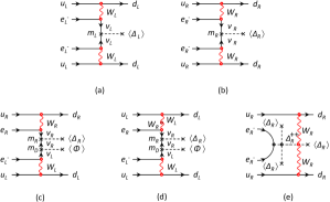
Figure 5: Possible flavor-basis contributions to $0\nu 2$EC within LRSM.

The Wilson coefficients $C^{K}_{n}$ in Eqs. (II.2) and (II.14) at the matching high-energy scale $\Lambda\sim M_{R}$ corresponding to the diagrams in Figs. 5(b)-(e) are given by

$$\mbox{Fig. \ref{fig:Fig-LRSM-1}~{}(b)}\sim y_{R}\langle\Delta_{R}\rangle \rightarrow C^{RR,N_{R}}_{3}\ =\sum_{i=1}^{3}U_{L\,ei}^{2}\frac{m_{p}}{m_{N_{i}}}\left(\frac{M_{W_{L}}}{M_{W_{R}}}\right)^{4}$$ (II.34)

$$\mbox{Fig. \ref{fig:Fig-LRSM-1}~{}(c)}\sim y_{\Phi}y_{R}\langle\Phi\rangle\langle\Delta_{R}\rangle \rightarrow C^{R,\hat{q}}_{3}=\sum_{i=1}^{3}U_{L\,ei}U_{D,ei}\left(\frac{M_{W_{L}}}{M_{W_{R}}}\right)^{2},$$ (II.35)

$$\mbox{Fig. \ref{fig:Fig-LRSM-1}~{}(d)}\sim\zeta_{W}y_{\Phi}y_{R}\langle\Phi\rangle\langle\Delta_{R}\rangle \rightarrow C^{L,\hat{q}}_{3}=\sum_{i=1}^{3}U_{L\,ei}U_{D,ei}\tan\zeta_{W},$$ (II.36)

$$\mbox{Fig. \ref{fig:Fig-LRSM-1}~{}(e)}\sim\lambda_{\Delta_{R}}g_{R}^{2}\langle\Delta_{R}\rangle \rightarrow C^{RR,\Delta^{++}_{R}}_{3}=\sum_{i=1}^{3}U_{R\,ei}^{2}\frac{m_{N_{i}}m_{p}}{m^{2}_{\Delta_{R}}}\left(\frac{M_{W_{L}}}{M_{W_{R}}}\right)^{4}.$$ (II.37)

Here, $\zeta_{W}$ is the angle of $W_{L}-W_{R}$-mixing. For convenience we showed the correspondence of the flavor-basis diagrams in Fig. 5 to the particular combinations of the parameters of the LRSM Lagrangian – quartic $\Delta_{R}$ coupling $\lambda_{\Delta_{R}}$, gauge coupling $g_{R}$ and VEV $\langle\Delta_{R}\rangle$ – and, then, give the corresponding Wilson coefficients.

$\bullet$ Leptoquark models: Leptoquarks (LQ) are exotic scalar or vector particles coupled to lepton-quark pairs in such a way $\bar{L}\cdot LQ\cdot Q$. They appear in various high-scale contexts, for example, in Grand Unification, extended Technicolor, Compositeness etc. For a generic LQ theory all the renormalizable interactions were specified by Buchmüller et al. (1987). Current experimental limits Tanabashi et al. (2018) allow them to be relatively light at the TeV scale. The SM gauge symmetry allows LQ to mix with the SM Higgs. This mixing generates $\Delta L=2$ interactions with the chiral structure leading to the long-range $\hat{q}$-type contribution not suppressed by the smallness of the Majorana mass $m_{\nu}$ of the light virtual neutrino displayed in the diagram of Fig. 6(a) with $S$ or $V$ being scalar or vector LQ. In the low-energy limit, the upper part of this diagram with heavy LQ reduces to the point-like vertex described by the operator $\mathcal{O}_{1}^{(6)X}$ in (II.3). The chirality structure of this vertex combined with the SM vertex in the bottom part render $\hat{q}$-type contribution to $0\nu 2$EC.

$\bullet$ R-parity violating supersymmetric models: The TeV-scale supersymmetric (SUSY) models offer a natural explanation of the GUT-SM scale hierarchy, introducing superpartners to each SM particle, so that they form supermultiplets (chiral superfields): $(q,\tilde{q})$, $(l,\tilde{l})$, $(g,\tilde{g})$ etc. Here $\tilde{q}$ and $\tilde{l}$ are scalar squarks and sleptons while $\tilde{g}$ is a spin-1/2 gluino. The SUSY framework requires at least two electroweak Higgs doublets $H_{U}$ and $H_{D}$. A class of SUSY models, the so called $R$-parity violating (RPV) SUSY models, allow for LNV interactions described by a superpotential

$$W_{RPV} = \lambda^{\prime}_{ijk}L_{i}Q_{j}\bar{D}_{k}+\epsilon_{i}L_{i}H_{U},$$ (II.38)

where $Q$, $D$ and $H_{U}$ conventionally denote here the chiral superfields of the left-chiral electroweak doublet quarks, the right-chiral electroweak singlet down quark and the up-type electroweak Higgs doublet, respectively.

The RPV SUSY models with the interactions (II.38) contribute to the long- and short range mechanisms of $0\nu 2$EC process. The corresponding diagrams are shown in Figs. 6. The first two diagrams generate the long-range $\hat{q}$-type contribution, while the last one with the gluino $\tilde{g}$ or neutralino $\chi$ exchange entail the short-range contribution. In the diagrams of Fig. 6(a,b) the source of LNV is located in the vertices of the upper part, while in Fig. 6(c) it is given by the Majorana mass of the neutralino $m_{\chi}$ and/or gluino $m_{\tilde{g}}$. In the low-energy limit the upper part of the diagrams in Fig. 6(a,b) lead to the operator $\mathcal{O}_{1}^{(6)L}$ while in this limit the diagram in Fig. 6(c), where all internal particles are heavy, collapses to a point-like short-range contribution given by a linear combination of d = 9 operators $\mathcal{O}_{1}^{(9)LL}$ and $\mathcal{O}_{2}^{(9)LL}$.

II.3 Hadronization of quark-level interactions

Let us comment on the calculation of the structure coefficients $\beta^{X}_{i},\beta^{XY}_{i}$ in the amplitude (II.14) depending on the NMEs and nucleon structure.

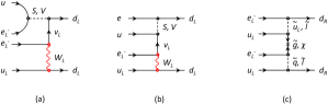
Figure 6: Possible flavor-basis contributions to $0\nu 2$EC within Leptoquark (a,b) and RPV MSSM (a,c) models. The cross $\times$ in diagram (c) denotes the Majorana mass of a gluino $\tilde{g}$ or neutralino $\chi$.

The Lagrangians (II.1) and (II.2) can, in principle, be applied to any LNV processes with whatever hadronic states: quarks, mesons, nucleons, other baryons, as well as nuclei. The corresponding amplitude, such as in Eq. (II.14), involves the hadronic matrix elements of the operators (II.6) and (II.5). The Wilson coefficients $C^{XY}_{i}$ are calculated in terms of the parameters of the high-scale model and are independent of the low-energy scale non-perturbative hadronic dynamics. This is the celebrated property of the operator product expansion, expressing interactions of some high-scale renormalizable model in the form of Eqs. (II.1) and (II.2) below a certain scale $\mu$. In the case of $0\nu 2\beta^{-}$ decay, $0\nu$2EC and other similar nuclear processes, the corresponding NMEs of the operators (II.6) and (II.5) are calculated in the framework of the approach based on non-relativistic impulse approximation (for a detailed description see, e.g., the paper of Doi et al. (1985)). This implies, as the first step, reformulating the quark-level theory in terms of the nucleon degrees of freedom, which the existing nuclear structure models operates with. This is the so-called hadronization procedure. In the absence of firm theory of hadronization one is left to resort upon general principles and particular models. Imbedding two initial(final) quarks into two different protons (neutrons) is conceptually a more simple option illustrated in Fig. 7(a). This is the conventional two-nucleon mechanism relying on the nucleon form factors as a phenomenological representation of the nucleon structure. On the other hand, putting one initial and one final quark into a charged pion while the other initial quark is put into a proton and one final quark into a neutron, as in Fig. 7(b), we deal with 1-pion mechanism. The 2-pion mechanism, displayed in Fig. 7 (c), treats all the quarks to be incorporated in two charged pions. In both cases the pions are virtual and interact with nucleons via the ordinary pseudoscalar pion-nucleon coupling $\bar{N}i\gamma_{5}\mbox{\boldmath$\tau$}\mbox{\boldmath$\pi$}N$. One may expect a priori dominance of the pion mechanism for the reason that it extends the region of the nucleon-nucleon interaction due to the smallness of the pion mass leading to a long-range potential. As a result, the suppression caused by the short-range nuclear correlation can be significantly alleviated in comparison to the conventional two-nucleon mechanism. Nevertheless, one should consider all these mechanisms to contribute to the process in question with corresponding relative amplitudes. The latter is as yet unknown. In principle, it can be evaluated in particular hadronic models. These kind of studies are still missing in literature and consensus on the dominance of one of these two mechanisms is pending. It is a common trend to posit the analysis on one of these two hadronization scenarios. Note that, for the long-range contributions described by the effective Lagrangian (II.1) the above-mentioned advantage of the pion mechanism is absent, and one can, in a sense, safely resort to the conventional two nucleon mechanism. The light Majorana exchange contribution to $0\nu 2$EC, on which we focus in the rest of this review, is of this kind. This limitation is explained by the fact that for the moment there are no yet Nuclear Matrix Elements calculated in the literature for other mechanisms different from this one.

The procedure of hadronization is essentially the same as for $0\nu\beta\beta$-decay and described in the literature. For more details on this approach to hadronization we refer readers to the original papers of Doi et al. (1985); Faessler et al. (1998, 2008) and the recent review by Graf et al. (2018).

Recently there has been developed another approach, which resorts to matching the high-scale quark-level theory to Chiral Perturbation Theory. The latter is believed to provide a low-energy description of QCD in terms of nucleon and pion degrees of freedom. It is expected that the parameters of the low-energy effective theory can be determined from experimental measurements or from the lattice QCD. This approach leads to quite different picture of hadronization and numerical results in comparison with the conventional approach sketched above. Surprisingly, contrary to the conventional approach short-range nucleon-nucleon interactions should be introduced for theoretical self-consistency even in the case of the long-range light neutrino exchange mechanism in Fig. 3(a). For the detailed description of this approach we refer the reader to the original papers of Prezeau et al. (2003); Graesser (2017); Cirigliano et al. (2019, 2017, 2018c, 2018b, 2018a) and the recent review of Cirigliano et al. (2020).

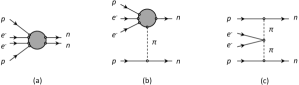
Figure 7: Hadron-level diagrams for $0\nu 2$EC: (a) the conventional two-nucleon mechanism, (b) the one-pion exchange and (c) the two-pion exchange mechanisms.

To conclude, neutrinoless double-electron capture $0\nu$2EC, the same as $0\nu\beta\beta$-decay, is a $\Delta L=2$ lepton number violating process. Moreover, at the level of nucleon sub-process it is virtually equal to $0\nu\beta\beta$-decay. Consequently, the underlying $\Delta L=2$ physics driving both these processes is the same. Obviously there are many formal differences in the form of the effective operators representing this physics at low energy sub-GeV scales. We specified a complete basis of the $0\nu$2EC effective operators in Eqs. (II.1)-(II.10) and exemplified high-energy scale models presently popular in the literature, which can be reduced to these operators in the low-energy limit. Akin to $0\nu\beta\beta$-decay there are basically three types of mechanisms of $0\nu$2EC shown in Fig. 3: (a) the conventional neutrino exchange mechanism with the amplitude proportional to the effective Majorana neutrino mass $m_{\beta\beta}$ defined in (II.12); (b) neutrino exchange mechanism independent of Majorana neutrino mass, when lepton number violation necessary for $0\nu$2EC to proceed is gained from a $\Delta L=2$ vertex; Both (a) and (b) are long-range mechanics induced by the exchange of a very light particle, a neutrino. On the other hand the diagram (d) represents a short-range mechanism induced by the exchange of heavy particles with masses much larger than the typical scale ($\sim$ few MeV) of $0\nu$2EC. Despite the underlying physics of both $0\nu$2EC and $0\nu\beta\beta$-decay is the same, their nuclear matrix elements (NME) are very different. We will discuss the nuclear structure aspects and atomic physics involved in the calculations of the $0\nu$2EC NMEs in the subsequent sections. Here it is worth noting that so far only the NMEs for the Majorana neutrino exchange mechanism Fig. 3(a) have been calculated in the literature. The similar calculations for NMEs of other mechanisms Fig. 3(b,c) are still pending.

III Phenomenology of neutrinoless 2EC

The diagrams in Figs. 1 and 2 can be combined as shown in Fig. 8. In the initial state, there is an atom $(A,Z)$. The electron lines belong to the electron shells, and the proton and neutron lines belong to the initial and intermediate nuclei, respectively. As a result of neutrinoless double-electron capture, an atom $(A,Z-2)^{**}$ is formed, generally in an excited state. In what follows, $(A,Z)^{*}$ denotes an atom with the excited electron shell, and $(A,Z)^{**}$ means that the nucleus is also excited. The intermediate atom can decay by emitting a photon or Auger electrons, but it can also experience $0\nu 2\beta^{-}$ transition and evolve back to the initial state. As a result, LNV oscillations $(A,Z)\leftrightarrow(A,Z-2)^{**}$ occur in the two-level system. These oscillations are affected by the coupling of the $(A,Z-2)^{**}$ atom to the continuum, which eventually leads to the decay of $(A,Z)$. The Hamiltonian of the system is not Hermitian because $(A,Z-2)^{**}$ has a finite width.

The LNV oscillations of atoms are discussed by Krivoruchenko et al. (2011); Šimkovic and Krivoruchenko (2009); Bernabeu and Segarra (2018). The formalism of LNV oscillations allows to find a relationship between the half-life $T_{1/2}$ of the initial atom $(A,Z)$, the amplitude of neutrinoless double-electron capture $V_{\alpha\beta}$, and the decay width of the intermediate atom $(A,Z-2)^{**}$, which has an electromagnetic origin.

III.1 Underlying formalism

The evolution of a system of mixed states, each of which may be unstable due to the coupling with the continuum, can described by an effective non-Hermitian Hamiltonian Weisskopf and Wigner (1930). In the case under consideration, the Hamiltonian takes the form

$$H_{\mathrm{eff}} = \left(\begin{array}[]{cc}M_{i}&V_{\alpha\beta}\\ V^{*}_{\alpha\beta}&M_{f}-\frac{i}{2}\Gamma_{f}\end{array}\right),$$ (III.3)

where $M_{i}$ and $M_{f}$ are the masses of the initial and final atoms. The width $\Gamma_{f}$ of the final excited atom with two vacancies $\alpha$ and $\beta$ is of electromagnetic origin. The off-diagonal matrix elements are due to a violation of lepton number conservation. They can be chosen real by changing the phase of one of the states; thus, we set $V_{\alpha\beta}=V^{*}_{\alpha\beta}$. The real and imaginary parts of the Hamiltonian do not commute.

Let us find the evolution operator

$$U(t)=\exp(-iH_{\mathrm{eff}}t).$$ (III.4)

According to Sylvester’s theorem, the function of a finite-dimensional $n\times n$ matrix $A$ is expressed in terms of the eigenvalues $\lambda_{k}$ of the matrix $A$, which are solutions of the characteristic equation $\det(A-\lambda)=0$, and a polynomial of $A$:

$$f(-iAt)=\sum_{k}f(-i\lambda_{k}t)\prod_{l\neq k}\frac{\lambda_{l}-A}{\lambda_{l}-\lambda_{k}},$$ (III.5)

where the sum runs over $1\leq k\leq n$, the product runs over $1\leq l\leq n$, $l\neq k$, and the eigenvalues are assumed to be pairwise distinct. The matrix function $f(-iAt)$ evolves with the time $t$ like the superposition of $n$ terms $f(-i\lambda_{k}t)$ with the matrix coefficients which are projection operators onto the $k$-th eigenstates of $A$.

The eigenvalues of the Hamiltonian (III.3) are equal to $\lambda_{\pm}=M_{+}\pm\Omega,$ where $M_{\pm}=(M_{i}\pm M_{f})/2\mp i\Gamma_{f}/4$, and $\Omega=\sqrt{V^{2}_{\alpha\beta}+M_{-}^{2}}$. The values of $\lambda_{\pm}$ are complex, so the norm of the states is not preserved in time. A series expansion around $V=0$ yields

$$\lambda_{+} \approx M_{i}+\Delta M-\frac{i}{2}\Gamma_{i},$$ (III.6)

$$\lambda_{-} \approx M_{f}-\Delta M-\frac{i}{2}(\Gamma_{f}-\Gamma_{i}),$$ (III.7)

with $\Delta M=(M_{i}-M_{f})\Gamma_{i}/{\Gamma_{f}}$, $\Gamma_{i}=V^{2}_{\alpha\beta}R_{f}$, and

$$R_{f}=\frac{\Gamma_{f}}{(M_{i}-M_{f})^{2}+\frac{1}{4}\Gamma_{f}^{2}}.$$ (III.8)

The initial state decays at the rate $\Gamma_{i}\ll\Gamma_{f}$. The width $\Gamma_{i}$ is maximal for complete degeneracy of the atomic masses:

$$\Gamma_{i}^{\max}=\frac{4V^{2}_{\alpha\beta}}{\Gamma_{f}}.$$ (III.9)

A simple calculation gives

$$U(t)=\exp(-iM_{+}t)\left(\cos(\Omega t)-i\frac{H_{\mathrm{eff}}-M_{+}}{\Omega}\sin(\Omega t)\right).$$ (III.10)

The decay widths of single-hole excitations of atoms are known experimentally and tabulated for $10\leq Z\leq 92$ and principal quantum numbers $1\leq n\leq 4$ by Campbell and Papp (2001). The width of a two-hole state $\alpha\beta$ is represented by the sum of the widths of the one-hole states $\Gamma_{f}=\Gamma_{\alpha}+\Gamma_{\beta}$. The de-excitation width of the daughter nucleus is much smaller and can be neglected. The values $\Gamma_{f}$ are used in estimating the decay rates $\Gamma_{i}$.

The transition amplitude from the initial to the final state for small time $t$, according to Eq. (III.10), is equal to

$$\langle f|U(t)|i\rangle=-iV_{\alpha\beta}t+...$$ (III.11)

This equation is valid for $t\lesssim 1/|M_{+}|$ and also over a wider range $t\lesssim 1/|\Omega|$, given that the real part of the phase can be made to vanish via redefinition of the Hamiltonian $H_{\mathrm{eff}}\to H_{\mathrm{eff}}-\Re(M_{+})$. The value of $V_{\alpha\beta}$ can be evaluated by means of field-theoretical methods that allow one to find the amplitude (III.11) from first principles. Formalism described in this subsection reproduces results of Bernabeu et al. (1983) with respect to $0\nu$2EC decay rates.

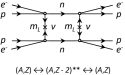
Figure 8: Oscillations of atoms induced by $0\nu 2$EC and $0\nu 2\beta$ transitions. The notations are the same as in Figs. 1 and 2. The intermediate atom $(A,Z-2)^{**}$ is coupled to the continuum through the emission of a photon and/or Auger electrons. These channels generate a finite width $\Gamma_{f}$ in Eq. (III.3), they are also responsible for the non-Hermitian character of $H_{\mathrm{eff}}$.

III.2 Decay amplitude of the light Majorana neutrino exchange mechanism

The total lepton number violation is due to the Majorana masses of the neutrinos. It is assumed that the left electron neutrino is a superposition of three left Majorana neutrinos:

$$\nu_{eL}=\sum^{3}_{i=1}U_{ek}\chi_{kL},$$ (III.12)

where $U$ is the PMNS mixing matrix. In the Majorana bispinor representation, $\chi_{kL}=\frac{1}{2}(1-\gamma_{5})\chi_{k}$ and $\chi_{k}^{*}=\chi_{k}.$ The vertex describing the creation and annihilation of a neutrino has the standard form

$${\cal H}(x)=\frac{G_{F}\cos{\theta_{C}}}{\sqrt{2}}j_{\mu}(x)J^{\mu}_{h}(x)+\mathrm{h.c.},$$ (III.13)

where ${\theta_{C}}$ is the Cabibbo angle. The lepton and quark charged currents are defined by Eq. (II.11). In terms of the composite fields, the hadron charged current is given by

$$J^{\mu}_{h}(x)=\bar{n}(x)\gamma^{\mu}(g_{V}-g_{A}\gamma_{5})p(x),$$ (III.14)

where $n(x)$ and $p(x)$ are the neutron and the proton field operators and $g_{{V}}=1$ and $g_{{A}}=1.27$ are the vector and axial-vector coupling constants, respectively. An effective theory could also include $\Delta$-isobars, meson fields and their vertices for decaying into lepton pairs and interacting with nucleons and each other.

As a result of the capture of electrons, the nucleus $(A,Z)$ undergoes a $0^{+}\to J^{\pi}$ transition. Conservation of total angular momentum requires that the captured electron pair be in the state $J$. In weak interactions, parity is not conserved; thus, it is not required that the parity of the electron pair be correlated with the parity of the daughter nucleus.

The wave function of a relativistic electron in a central potential has the form

$$\Psi_{\alpha m_{\alpha}}(\mathbf{r})=\left(\begin{array}[]{l}f_{\alpha}(r)\Omega_{\alpha m_{\alpha}}(\mathbf{n})\\ ig_{\alpha}(r)\Omega_{\alpha^{\prime}m_{\alpha}}(\mathbf{n})\end{array}\right),$$ (III.15)

where $\alpha=(njl)$, $\alpha^{\prime}=(njl^{\prime}),$ $l^{\prime}=2j-l$. The radial wave functions are defined in agreement with Berestetsky et al. (1982); $\Omega_{\alpha m_{\alpha}}(\mathbf{n})\equiv\Omega_{jm_{\alpha}}^{l}(\mathbf{n})$, $\Omega_{\alpha^{\prime}m_{\alpha}}(\mathbf{n})=\Omega_{jm_{\alpha}}^{l^{\prime}}(\mathbf{n})$ are spherical spinors in the notations of Varshalovich et al. (1988). The normalization condition for $\Psi_{\alpha m_{\alpha}}(\mathbf{r})$ is given by

$$\int d\mathbf{r}\Psi_{\alpha m_{\alpha}}^{\dagger}(\mathbf{r})\Psi_{\beta m_{\beta}}(\mathbf{r})=\delta_{\alpha\beta}\delta_{m_{\alpha}m_{\beta}}.$$ (III.16)

If the captured electrons occupy the states $\alpha\equiv(n2jl)_{1}$ and $\beta\equiv(n2jl)_{2}$, we must take the superposition of products of their wave functions:

$$\psi_{\alpha\beta}^{JM}(\mathbf{r}_{1},\mathbf{r}_{2})=\sum_{m_{\alpha}m_{\beta}}C_{j_{\alpha}m_{\alpha}j_{\beta}m_{\beta}}^{JM}\Psi_{\alpha m_{\alpha}}(\mathbf{r}_{1})\Psi_{\beta m_{\beta}}(\mathbf{r}_{2}),$$ (III.17)

where $j_{\alpha}$ and $j_{\beta}$ are the total angular momenta, $m_{\alpha}$ and $m_{\beta}$ are their projections on the direction of the $z$ axis, and $\Psi_{\alpha m_{\alpha}}(\mathbf{r})$ and $\Psi_{\beta m_{\beta}}(\mathbf{r})$ are the relativistic wave functions of the bound electrons in an electrostatic mean field of the nucleus and the surrounding electrons. The identity of the fermions implies that the wave function of two fermions is antisymmetric; thus, the final expression for the wave function takes the form

$$\Psi_{\alpha\beta}^{JM}(\mathbf{r}_{1},\mathbf{r}_{2})=\mathcal{N}_{\alpha\beta}(\psi_{\alpha\beta}^{JM}(\mathbf{r}_{1},\mathbf{r}_{2})-(-)^{j_{\alpha}+j_{\beta}-J}\psi_{\beta\alpha}^{JM}(\mathbf{r}_{1},\mathbf{r}_{2})),$$ (III.18)

where $\mathcal{N}_{\alpha\beta}$ equals ${1}/{\sqrt{2}}$ for $\alpha\neq\beta$ and ${1}/2$ for $\alpha=\beta$.

As a consequence of the identity $C_{jm_{1}jm_{2}}^{JM}=(-1)^{J-2j}C_{jm_{2}jm_{1}}^{JM}$, the wave function of two electrons with equal quantum numbers $\alpha=\beta$ is symmetric under the permutation $m_{\alpha}\leftrightarrow m_{\beta}$ provided their angular momenta are combined to the total angular momentum $J=2j$ mod(2). In such a case, the antisymmetrization (III.18) yields zero, which means that the states $J=2j$ mod(2) are nonexistent. The antisymmetrization (III.18) of the states $J=2j+1$ mod(2) leads to a doubling of the initial wave function. To keep the norm, the additional factor $1/\sqrt{2}$ is thus required for $\alpha=\beta$.

The derivation of the equation for $V_{\alpha\beta}$ is analogous to the corresponding derivation of the $0\nu 2\beta$ decay amplitude, as described in the review of Bilenky and Petcov (1987). The specificity is that a transition from a discrete level to a quasi-discrete level is considered. Accordingly, the delta function expressing the energy conservation is replaced by a time interval that can be identified with the parameter $t$ in Eq. (III.11). We thus write

$$\langle f|\mathcal{U}(t)|i\rangle=-iV_{\alpha\beta}t+...,$$ (III.19)

where $\mathcal{U}(t)$ is Dyson’s $U$-matrix. The amplitude takes the form

$$V_{\alpha\beta} = iK_{Z}m_{\beta\beta}\sqrt{2}\mathcal{N}_{\alpha\beta}\left(\frac{G_{F}\cos\theta_{C}}{\sqrt{2}}\right)^{2}\int\frac{d\mathbf{q}}{(2\pi)^{3}}d{\mathbf{r}}_{1}d{\mathbf{r}}_{2}\frac{1}{\sqrt{2J+1}}\sum_{M}\frac{e^{-i\mathbf{q}({\mathbf{r}}_{1}-{\mathbf{r}}_{2})}}{2q_{0}}$$

$$\times \left[T^{JM}_{\mu\nu\alpha\beta}({\mathbf{r}}_{1},{\mathbf{r}}_{2})N^{\mu\nu}_{JM\alpha\beta}({\mathbf{r}}_{1},{\mathbf{r}}_{2})-(-1)^{j_{\alpha}+j_{\beta}-J}T^{JM}_{\mu\nu\beta\alpha}({\mathbf{r}}_{1},{\mathbf{r}}_{2})N^{\mu\nu}_{JM\beta\alpha}({\mathbf{r}}_{1},{\mathbf{r}}_{2})\right],$$

where

$$T^{JM}_{\mu\nu\alpha\beta}({\mathbf{r}}_{1},{\mathbf{r}}_{2}) = \sum_{m_{\alpha}m_{\beta}}C^{JM}_{j_{\alpha}m_{\alpha}j_{\beta}m_{\beta}}\left[{\bar{\Psi}_{\alpha m_{\alpha}}^{c}}({\mathbf{r}}_{1})\gamma_{\mu}(1+\gamma_{5})\gamma_{\nu}{\Psi_{\beta m_{\beta}}}({\mathbf{r}}_{2})\right],$$

$$N^{\mu\nu}_{JM\alpha\beta}({\mathbf{r}}_{1},{\mathbf{r}}_{2}) = \sum_{n}\left[\frac{\langle JM|J^{\mu}_{h}({\mathbf{r}}_{1})|n\rangle\langle n|J^{\nu}_{h}({\mathbf{r}}_{2})|00\rangle}{q_{0}+E_{n}-M_{i}-\varepsilon_{\beta}}+\frac{\langle JM|J^{\nu}_{h}({\mathbf{r}}_{2})|n\rangle\langle n|J^{\mu}_{h}({\mathbf{r}}_{1})|00\rangle}{q_{0}+E_{n}-M_{i}-\varepsilon_{\alpha}}\right].$$

Here, $q_{0}\approx|\mathbf{q}|$, $\langle JM|=\langle f|$ and $|00\rangle=|i\rangle$ are the states of the final and initial nuclei, respectively; $\varepsilon_{\gamma}=m-\varepsilon_{\gamma}^{*}$, $\varepsilon_{\gamma}^{*}$ is the one-hole excitation energy of the initial atom. The sum is taken over all excitations of the intermediate atom $(A,Z-1)$. In the Majorana bispinor representation, $\Psi_{\alpha m_{\alpha}}^{c}=\Psi_{\alpha m_{\alpha}}^{*}$. The amplitude $V_{\alpha\beta}$ is a scalar under rotation. By virtue of identities

$$T^{JM}_{\mu\nu\alpha\beta}({\mathbf{r}}_{1},{\mathbf{r}}_{2}) = -(-1)^{j_{\alpha}+j_{\beta}-J}T^{JM}_{\nu\mu\beta\alpha}({\mathbf{r}}_{2},{\mathbf{r}}_{1}),$$

$$N^{\mu\nu}_{JM\alpha\beta}({\mathbf{r}}_{1},{\mathbf{r}}_{2}) = N^{\nu\mu}_{JM\beta\alpha}({\mathbf{r}}_{2},{\mathbf{r}}_{1}),$$

$V_{\alpha\beta}$ is also invariant under permutations of $\alpha$ and $\beta$. For $\alpha=\beta$ and $J=2j_{\alpha}+1$ mod(2), the second term in the square brackets of Eq. (III.2) doubles the result, whereas for $\alpha=\beta$ and $J=2j_{\alpha}$ mod(2), $V_{\alpha\beta}=0$. The factor $\mathcal{N}_{\alpha\beta}$ provides the correct normalization.

In the processes associated with the electron capture, shell electrons of the parent atom appear in a superposition of the stationary states of the daughter atom. The overlap amplitude of two atoms with atomic numbers $Z$ and $Z+\Delta Z$ can be evaluated for $\Delta Z\ll Z$ in a simple non-relativistic shell model to give Krivoruchenko and Tyrin (2020)

$$K_{Z}\approx\exp\left(-{\frac{3^{5/3}2^{1/3}}{80}}\frac{\Delta Z^{2}}{Z^{1/3}}\right).$$ (III.21)

The overlap factors for ⁹⁶Ru, ¹⁵²Gd and ¹⁹⁰Pt atoms, e.g., equal $K_{Z}=0.895$, $0.906$, and $0.912$, respectively. The result is not very sensitive to the charge. Valence-shell electrons are involved in the formation of chemical bonds and give an important contribution to $K_{Z}$. We limit ourselves to estimating the core-shell electrons contribution which weakly depends on the environment.

The weak charged current of a nucleus for a low-energy transfer can be written in the form

$$J^{\mu}(0,\mathbf{r})=\sum_{a}\tau^{-}_{a}[g_{V}g^{\mu 0}+g_{A}(\sigma_{k})_{a}g^{\mu k}]\delta(\mathbf{r}-{\mathbf{r}}_{a}).$$ (III.22)

This approximation neglects the contribution of the exchange currents. The short-term contribution of some higher-dimensional operators is dominated by the pion exchange mechanism (see, e.g., the paper of Faessler et al. (2008)).

The neutrino momentum enters the energy denominators of Eq. (III.2). The typical value of $q_{0}$ is of the order of the Fermi momentum, $p_{F}=270$ MeV. The remaining quantities in the energy denominators are of the order of the nucleon binding energy in the nucleus $\sim 8$ MeV, i.e., substantially lower. The energy denominators can therefore be taken out from the square bracket such that the sum over the excited states can be performed using the completeness condition $\sum_{n}|n\rangle\langle n|$ = 1. This approximation is called the closure approximation. The integral over $\mathbf{q}$ entering Eq. (III.2) with good accuracy is inversely proportional to the distance between two nucleons. The decay amplitude can finally be written in the form (cf. Krivoruchenko et al. (2011))

$$V_{\alpha\beta}\approx G_{F}^{2}\cos^{2}\theta_{C}K_{Z}m_{\beta\beta}\frac{g^{2}_{A}}{4\pi R}\sqrt{2J_{f}+1}M^{\mathrm{2EC}}{\cal A}_{\alpha\beta}.$$ (III.23)

Here, the electron and nuclear parts of the amplitude are assumed to factorize. Such an approximation is well justified in the case of $K$ capture given the approximate constancy of the electron wave functions inside the nucleus. The still-probable capture of an electron from the $p_{1/2}$ state is determined by the lower dominant component of the electron wave function inside the nucleus, which is also approximately constant. The factorization is also supported by the fact of localization of nucleons involved in the decay near the nuclear surface.

The decay amplitude due to the operators of higher dimension of Fig. 3 (b,c) has the form of Eq. (III.23) with the replacement

$$m_{\beta\beta}\frac{g_{A}^{2}}{4\pi R}\sqrt{2J_{f}+1}M^{\mathrm{2EC}}\rightarrow\sum_{i=1}^{3}\beta_{i}^{X}(\mu_{0},\Lambda)C_{i}^{X}(\Lambda)+\sum_{i=1}^{5}\beta_{i}^{XY}(\mu_{0},\Lambda)C_{i}^{XY}(\Lambda).$$ (III.24)

The value of $\mathcal{A}_{\alpha\beta}$ entering Eq. (III.23) is the product of electron wave functions, whose bispinor indices are contracted in a way depending on the type of nuclear transition and the type of operator responsible for the decay.

For neutrino exchange mechanism, the explicit expressions for ${\cal A}_{\alpha\beta}$ of low-$J$ nuclear transitions $0^{+}\to 0^{\pm},1^{\pm}$ in terms of the upper and lower radial components of the electron wave functions are given by Krivoruchenko et al. (2011). For $j_{\alpha}=j_{\beta}=1/2$ and arbitrary $n_{\alpha}$ and $n_{\beta}$, one gets

$${\mathcal{A}}_{\alpha\beta}(0^{+}\to 0^{+}) = \langle F^{(+)}_{\alpha\beta}(r_{a},r_{b})\rangle,$$ (III.25)

$${\mathcal{A}}_{\alpha\beta}(0^{+}\to 0^{-}) = \langle H^{(+)}_{\alpha\beta}(r_{a},r_{b})\rangle,$$ (III.26)

$${\mathcal{A}}_{\alpha\beta}(0^{+}\to 1^{+}) \approx \langle F^{(-)2}_{\alpha\beta}(r_{a},r_{b})\rangle^{1/2},$$ (III.27)

$${\mathcal{A}}_{\alpha\beta}(0^{+}\to 1^{-}) \approx \langle(H^{(-)}_{\alpha\beta}(r_{a},r_{b})-H^{(-)}_{\alpha\beta}(r_{b},r_{a}))^{2}/4\rangle^{1/2}.$$ (III.28)

The functions $F^{(\pm)}$ and $H^{(\pm)}$ depend on the radial variables $r_{a}$ and $r_{b}$ and quantum numbers $\alpha$ and $\beta$ of the captured electrons. For $l_{\alpha}=l_{\beta}=0$, one finds $4\pi F_{\alpha\beta}^{(\pm)}(r_{a},r_{b})=\mathcal{N}_{\alpha\beta}(f_{\alpha}(r_{a})f_{\beta}(r_{b})\pm f_{\beta}(r_{a})f_{\alpha}(r_{b}))$ and $4\pi H^{(\pm)}_{\alpha\beta}(r_{a},r_{b})=\mathcal{N}_{\alpha\beta}(g_{\alpha}(r_{a})f_{\beta}(r_{b})\pm g_{\beta}(r_{a})f_{\alpha}(r_{b}))$. Computation of electron radial wave functions $f_{\alpha}(r)$ and $g_{\alpha}(r)$ is discussed in Sec. IV. Nuclear structure models for matrix elements $M^{\mathrm{2EC}}$ entering Eq. (III.23) are discussed in Sec. V.

III.3 Comparison of $0\nu$2EC and $0\nu 2\beta^{-}$ decay half-lives

Here, we obtain estimates for half-lives of the $0\nu$2EC and $0\nu 2\beta^{-}$ decay, starting from the expressions of the paper of Suhonen and Civitarese (1998). The inverse $0\nu 2\beta^{-}$ half-life can be written in the form

$$\left(T_{1/2}^{0\nu 2\beta}\right)^{-1}=\left(\frac{|m_{\beta\beta}|}{m}\right)^{2}|{M}_{2\beta}|^{2}G_{2\beta},$$ (III.29)

where ${M}_{2\beta}$ is the nuclear matrix element of the $0\nu 2\beta^{-}$ decay, $m$ is the electron rest mass, $G_{2\beta}=g_{\mathrm{A}}^{4}K_{Z}^{2}g^{(0\nu)}r_{A}^{-2}\mathcal{I}\$ is the phase-space factor, with $r_{A}=mR$, $R=1.2A^{1/3}\,\text{fm}$ being the nuclear radius. $K_{Z}$ describes the overlap of the electron shells of the parent and daughter atoms including the possible ionization of the latter. In what follows, we neglect the electron shell effects and set $K_{Z}=1$. The factor $g^{(0\nu)}=2.80\times 10^{-22}\,$y^-1 includes all the fundamental constants and other numerical coefficients entering the half-life. The phase-space integral reads

$$\mathcal{I}=\int_{1}^{\tilde{Q}+1}F_{0}(Z_{f},\varepsilon_{1})F_{0}(Z_{f},\varepsilon_{2})p_{1}p_{2}\varepsilon_{1}\varepsilon_{2}d\varepsilon_{1},$$ (III.30)

where $\varepsilon_{1,2}$ are the total energies and $p_{1,2}$ the momenta of the emitted electrons, scaled by the electron mass. Here $\tilde{Q}=Q/m$ is the normalized $Q$ value of the decay. The quantities $F_{0}(Z_{f},\varepsilon)$ are the Fermi functions taking into account the Coulomb interaction between the emitted electrons and the final nucleus with charge number $Z_{f}$. The integral $\mathcal{I}$ can be integrated analytically by noticing that $\varepsilon_{2}=\tilde{Q}+2-\varepsilon_{1}$ and using the Primakoff-Rosen approximation $F_{0}(Z_{f},\varepsilon)=(\varepsilon/p)F_{0}^{\mathrm{(PR)}}(Z_{f}).$ This leads in a good approximation to $\mathcal{I}\approx 10\pi^{2}\alpha^{2}Z_{f}^{2}(\tilde{Q}+1)^{5}/3$ (cf. Suhonen and Civitarese (1998)) and to the corresponding phase-space factor $G_{2\beta}=g_{\mathrm{A}}^{4}Z_{f}^{2}A^{-2/3}(\tilde{Q}+1)^{5}~{}5\times 10^{-20}\,\mathrm{y}^{-1}$. Combining with the rest of the $0\nu 2\beta$ observables, the inverse half-life can be written as

$$\left(T_{1/2}^{0\nu 2\beta}\right)^{-1}=g_{\mathrm{A}}^{4}\left(\frac{|m_{\beta\beta}|}{m}\right)^{2}|{M}_{2\beta}|^{2}Z_{f}^{2}A^{-2/3}(\tilde{Q}+1)^{5}\,5.0\times 10^{-20}\text{y}^{-1}.$$ (III.31)

The inverse $0\nu$2EC half-life is given by

$$\left(T_{1/2}^{0\nu 2\text{EC}}\right)^{-1}=\Gamma_{i}/\ln 2\equiv G_{\mathrm{2EC}}R_{f},$$ (III.32)

where $G_{\mathrm{2EC}}=V_{\alpha\beta}^{2}/\ln 2,$ and $R_{f}$ is defined by Eq. (III.8). For $J_{f}^{\pi}=0^{+}$ and $K_{Z}=1$, we find in the non-relativistic approximation for two-electron capture from the lowest $K$ shell

$$\left(T_{1/2}^{0\nu 2\text{EC}}\right)^{-1}=g_{\mathrm{A}}^{4}\left(\frac{|m_{\beta\beta}|}{m}\right)^{2}|M_{\mathrm{2EC}}|^{2}Z_{i}^{6}A^{-2/3}\alpha^{2}mR_{f}\,5.1\times 10^{-25}\text{y}^{-1},$$ (III.33)

where $M_{\mathrm{2EC}}$ is the $0\nu$2EC nuclear matrix element.

We can now find the ratio of the two processes. Adopting the simplification $Z_{f}\approx Z_{i}\equiv Z$ and assuming $\mathrm{M}_{2\beta}\approx M_{\mathrm{2EC}}$, one finds for the half-life ratio

$$\frac{T_{1/2}^{0\nu 2\text{EC}}}{T_{1/2}^{0\nu 2\beta}}\approx\left(\frac{20}{Z}\right)^{4}\frac{(\tilde{Q}+1)^{5}}{\alpha^{2}mR_{f}}.$$ (III.34)

Given that $\Gamma_{f}\sim\alpha^{2}m=27.2$ eV, one immediately derives that the two processes have comparable half-lives for $\alpha^{2}mR_{f}\sim 1$ which is the case for $|M_{i}-M_{f}|\lesssim\Gamma_{f}$.

IV Electron shell effects

The selection of atoms with near-resonant $0\nu 2$EC transitions requires an accurate value of the double-electron ionization potentials of the atoms and the electron wave functions in the nuclei. The electron shell models are based on the Hartree-Fock and post-Hartree-Fock methods, density functional theory, and semiempirical methods of quantum chemistry. Analytical parametrizations of the non-relativistic wave functions of electrons in neutral atoms, obtained with the use of the Roothaan-Hartree-Fock method and covering almost the entire periodic table, are provided by Clementi and Roetti (1974); McLean and McLean (1981); Snijders et al. (1981); Bunge et al. (1993). The various feasible $0\nu 2$EC decays are expected to occur in medium-heavy and heavy atoms, for which relativistic effects are important. With the advent of personal computers, physicists acquired the opportunity to use advanced software packages, such as Grasp2K Dyall et al. (1989); Grant (2007), DIRAC , CI-MBPT Kozlov et al. (2015) and others, for applications of relativistic computational methods in modeling complex atomic systems.

Quantum electrodynamics (QED) of electrons and photons is known to be a self-consistent theory within infinite renormalizations. One could expect the existence, at least, of a similarly formally consistent theory of electrons, photons and nuclei, regarded as elementary particles, which would be a satisfactory idealization for most practical purposes.

In quantum field theory, the relativistic bound states of two particles are described by the Bethe-Salpeter equation Salpeter and Bethe (1951); Hayashi and Munakata (1952). In the nonrelativistic limit, this equation leads to the Schrödinger wave equation, but it also includes additional anomalous solutions that do not have a clear physical interpretation: First, there are bound states corresponding to excitations of the time-like component of the relative four momenta of the particles. Such states have no analogs in the nonrelativistic potential scattering theory. None of the particles observed experimentally have been identified with the anomalous solutions so far. Second, some solutions appear with a negative norm. Third, the Bethe-Salpeter kernel, evaluated at any finite order of perturbation theory, breaks crossing symmetry and gauge invariance of QED Nakanishi (1969); Itzykson and Zuber (1980). The anomalous solutions do not arise when retardation effects are neglected.

Applications of the Bethe-Salpeter equation to hydrogen atom Salpeter (1952) and positronium Itzykson and Zuber (1980) appeared to be successful because of the non-relativistic character of the bound-state problems and the possibility to account for the retardation effects with the help of perturbation theory in terms of the small parameter $1/c$.

A successful attempt at generalization of the series expansion around the instantaneous approximation to multielectron atoms is presented in the papers of Sucher (1980); Broyles (1988), where the progress was achieved by using non-covariant perturbation theory in the coupling constant, $\alpha$, of electrons with the transverse part of the electromagnetic vector potential and the magnitude of $Z$ diagrams describing creation and annihilation of electron-positron pairs. Such a perturbation theory appears well-founded because the transverse components of the electromagnetic vector potential interact with spatial components of the electromagnetic current, which contain the small term $1/c$, whereas $Z$ diagrams contribute to observables in higher orders of $1/c$. Compared with lowest-order Coulomb photon exchange diagrams, $Z$ diagrams are suppressed by the factors ${u}^{\dagger}v^{\prime}\sim 1/c$ or ${v}^{\prime\dagger}u\sim 1/c$ in each of the photon vertices due to overlapping of the small and large bispinor components and the factor $1/c^{2}$ originating from the propagator of the positron. As a result, $Z$ diagrams are of the order $O(\alpha^{2}/c^{4})$. The second-order correction to the energy due to the Fermi-Breit potential is of the same magnitude. The exchange of transverse photons leading to the Fermi-Breit potential contributes to the interaction potential of order $\alpha/c^{2}$, such that the magnitude of the $Z$ diagrams is suppressed. The scheme adopted by Sucher (1980); Broyles (1988) is equivalent to neglecting the Dirac sea at the zeroth-order approximation, except for the two-body problem, in which the bound-state energy equation is the same as in the paper of Salpeter (1952). The non-sea approximation is widely used to study nuclear matter in the Dirac-Brueckner-Hartree-Fock method Anastasio et al. (1983); Brockmann and Machleidt (1984); Ter Haar and Malfliet (1987). Let us remark that the negative-energy fermion states are required to ensure causality and guarantee Lorentz invariance of the $T$-product and hence of the $S$-matrix.

The self-consistent non-relativistic expansion becomes possible because the corrections related to the finite speed of light are small. The neglect of retardation allows for the formulation of an equation for the Bethe-Salpeter wave function integrated over the relative energy of the particles Broyles (1988). The non-covariant wave function obtained in this manner yields the wave function of the equivalent many-body non-covariant Schrödinger equation. Gauge invariance of QED ensures Lorentz invariance of the theory, but in the intermediate stages of the computation, it is necessary to work with Lorentz-noncovariant and gauge-dependent expressions.

In the Feynman gauge, the product of two photon vertices and the photon propagator

$$D_{\mu\nu}(k)=\frac{-g_{\mu\nu}}{k^{2}}$$ (IV.1)

is represented as follows:

$$e\gamma_{1}^{\mu}D_{\mu\nu}(k)e\gamma_{2}^{\nu}=-\gamma_{1}^{0}\gamma_{2}^{0}\frac{e^{2}}{k^{2}}\left(1-\mbox{\boldmath$\alpha$}_{1}\cdot\mbox{\boldmath$\alpha$}_{2}\right),$$ (IV.2)

where $k=(\omega,\mathbf{k})$ is the photon momentum, $\mbox{\boldmath$\alpha$}_{i}=\gamma_{i}^{0}\mbox{\boldmath$\gamma$}_{i}$ are velocity operators for the particles $i=1,2$, and $\gamma^{\mu}$ are the Dirac $\gamma$-matrices. The corresponding interaction potential obtained in the static limit,

$$V_{CG}(\mathbf{r}) \equiv \int\frac{d\mathbf{k}}{(2\pi)^{3}}\exp(i\mathbf{k}\mathbf{r})e\gamma_{1}^{0}\gamma_{1}^{\mu}D_{\mu\nu}(\omega=0,\mathbf{k})e\gamma_{2}^{0}\gamma_{2}^{\nu}$$ (IV.3)

$$= \frac{e^{2}}{4\pi r}\left(1-\mbox{\boldmath$\alpha$}_{1}\cdot\mbox{\boldmath$\alpha$}_{2}\right),$$

acquires familiar form of electrostatic interaction energy of charges plus magnetostatic interaction energy of electric currents. The correction to the Coulomb potential entering Eq. (IV.3) was first derived quantum-mechanically by Gaunt (1929). The expansion of $D_{\mu\nu}(k)$ in higher powers of $\omega$ describes retardation effects, which are expected to be most pronounced for inner orbits. A typical splitting of the energy levels is $\omega\sim\alpha^{2}Z^{2}m$, and a typical momentum of electrons is $|\mathbf{k}|\sim\alpha Zm$, such that for light and medium-heavy atoms, the expansion parameter $\omega^{2}/\mathbf{k}^{2}\sim(\alpha Z)^{2}$ is still sufficiently small. The potential of Eq. (IV.3) is known as the Coulomb-Gaunt potential. Such a potential can be used to approximate the lowest-order interaction of electrons, although the magnetostatic energy $\sim 1/c^{2}$ is of the same order as the retardation corrections to the Coulomb potential.

In the Coulomb gauge, the photon propagator $D_{\mu\nu}(k)$ takes the form

$$D_{00}(k) = \frac{1}{\mathbf{k}^{2}},$$

$$D_{ij}(k) = \frac{\delta_{ij}-k_{i}k_{j}/\mathbf{k}^{2}}{k^{2}},$$ (IV.4)

$$D_{i0}(k) = D_{0j}(k)=0,$$

where $i,j=1,2,3$. The Coulomb gauge breaks Lorentz covariance but appears natural in the problem of quantization of the electromagnetic field, since it allows for explicitly solving the constraint equations. The photon propagator appears split in two pieces, the first of which corresponds to the instantaneous interaction; the second describes the static terms $\sim 1/c^{2}$ plus retardation effects $\sim 1/c^{4}$. The potential of a zero-order approximation contains contributions from the time-like components and the space-like component of the propagator in the limit of $\omega=0$. The product of two photon vertices and the propagator (IV.4) is represented by

$$e\gamma_{1}^{\mu}D_{\mu\nu}(k)e\gamma_{2}^{\nu}=\gamma_{1}^{0}\gamma_{2}^{0}\left(\frac{e^{2}}{\mathbf{k}^{2}}+\frac{e^{2}}{k^{2}}\left(\mbox{\boldmath$\alpha$}_{1}\cdot\mbox{\boldmath$\alpha$}_{2}-\frac{\mbox{\boldmath$\alpha$}_{1}\cdot\mathbf{k}\mbox{\boldmath$\alpha$}_{2}\cdot\mathbf{k}}{\mathbf{k}^{2}}\right)\right).$$ (IV.5)

The interaction potential corresponding to the static limit of Eq. (IV.5) becomes

$$V_{CB}(\mathbf{r})=\frac{e^{2}}{4\pi r}\left(1-\frac{\mbox{\boldmath$\alpha$}_{1}\cdot\mbox{\boldmath$\alpha$}_{2}+\mbox{\boldmath$\alpha$}_{1}\cdot\mathbf{n}\mbox{\boldmath$\alpha$}_{2}\cdot\mathbf{n}}{2}\right),$$ (IV.6)

where $\mathbf{n}=\mathbf{r}/|\mathbf{r}|$. Equation (IV.6) can be recognized as the sum of the classical Coulomb and Darwin potentials Darwin (1920), which demonstrates the essentially classical origin of $V_{CB}$. The no-sea approximation is thus sufficient to ensure the correct expression for $V_{CB}$. The potential $V_{CB}$ given by Eq. (IV.6) was derived first quantum-mechanically by Breit (1929); it is known as the Coulomb-Breit potential. Starting with $V_{CB}$ is a natural choice, since the retardation effects in this case are of the order of $1/c^{4}$.

The techniques of Sucher (1980); Broyles (1988) can be considered as the starting point for developing a systematic $1/c$ expansion around the instantaneous approximation in the bound-state problem for light and medium-heavy atoms in analogy with positronium and the hydrogen atom. Heavy atoms for which the expansion parameter $1/c$ is not small are somewhat beyond the scope of perturbational treatment. Since theoretical estimates of accuracy are difficult, it is required to compare model predictions with empirical data wherever possible.

The relativistic approach is based on the Dirac-Coulomb Hamiltonian,

$$H=\sum_{i}\left(\mbox{\boldmath$\alpha$}\mathbf{p}_{i}+\beta m-\frac{\alpha Z}{r_{i}}\right)+\sum_{i<j}V(\mathbf{r}_{i}-\mathbf{r}_{j}),$$ (IV.7)

where the sum runs over electrons, $r_{i}=|\mathbf{r}_{i}|$. The potential $V(\mathbf{r})$ is, as a rule, taken to be the Coulomb-Breit potential, which already accounts for relativistic effects $\sim 1/c^{2}$ at the lowest order of the perturbation expansion. Neglecting the Dirac sea could require the projection of the potential onto positive energy states. The electron wave function is constructed as a Slater determinant of one-electron orbitals. Solutions to the eigenvalue problem are sought using the Dirac-Hartree-Fock approximation.

In the non-relativistic Coulomb problem, physical quantities are determined by a one-dimensional parameter, which is the Bohr radius, $a_{B}=1/(\alpha m)=5.2\times 10^{4}$ fm. In the relativistic problem, the Bohr radius acts as a scale, which determines the normalization of electron wave functions and the integral characteristics, such as the interaction energies of holes in the electron shell. In addition to the Bohr radius, there are other scales of the relativistic problem. The electron Compton wavelength $\lambda_{e}=1/m$ determines the distance from the nucleus, at which the electron should be considered in a relativistic manner. On a scale smaller than $1/m$, the non-relativistic wave function is markedly different from the upper component of the Dirac wave function; thus, the effects associated with the finite size of the nucleus must be calculated on the basis of the relativistic Dirac equation. The third scale in the hierarchy is the distance $\alpha Z/m=2.8Z$ fm, at which the Coulomb potential becomes greater than the electron mass. The smallest (fourth) scale is the nuclear radius $R=1.2A^{1/3}$ fm. The size of the ²³⁸U nucleus, e.g., is approximately 35 times smaller than $\alpha Z/m=260$ fm, approximately 50 times smaller than the Compton wavelength $1/m=390$ fm, and approximately 75 times smaller than $1/(\alpha mZ)=580$ fm. The depth of the potential extending from $0$ to $\alpha Z/m$ is too small to produce bound states of electrons in the negative continuum.

According to the Thomas-Fermi model, the majority of the shell electrons are at a distance $1/(\alpha mZ^{1/3})$ from the nucleus, and the total binding energy of the electrons scales as 20.8$Z^{7/3}$ eV. The potential energy of the interaction of electrons with each other is 1/7 of the energy of the interaction of electrons with the nucleus. The numerical smallness of the electron-electron interaction shows that the Coulomb wave functions of electrons can be used as a first approximation to the self-consistent mean-field solutions.

The single-electron ionization potentials (SEIP) of innermost orbits, which are of specific interest to the $0\nu 2$EC problem, increase quadratically with $Z$ from 13.6 eV in the hydrogen atom up to 115.6 keV in the uranium atom. The radii of the outer orbits and hence the size of atoms do not depend on $Z$. The SEIPs of outermost orbits are of the order of a few eV for all $Z$. The greatest overlap with the nucleus is achieved for electrons of the innermost orbits. In the $(A,Z)\to(A,Z-2)$ transitions associated with the $0\nu 2$EC decays, we are interested in the electron wave functions inside the parent nucleus $(A,Z)$, whereas the energy balance is provided by the energy of the excited electron shells of the daughter nucleus $(A,Z-2)$. The SEIPs of all orbitals across the entire periodic table are given by Larkins (1977), where experimental data on the binding energy of electron subshells and data obtained from Hartree-Fock atomic calculations are combined within a general semi-empirical method.

The double-electron ionization potentials (DEIPs) are additive to first approximation. A more accurate estimate of DEIPs takes account of interaction energy of electron holes, relaxation energy and other specific effects. In the innermost orbitals, the Coulomb interaction energy of two holes is of the order $\alpha Z/a_{B}\sim\alpha^{2}Zm$. This energy grows linearly with $Z$ and reaches a value of $\sim 1$ keV in heavy atoms. Relaxation energy for a medium-heavy atom of ¹⁰¹Ru reaches a value of 400 eV Niskanen et al. (2011). The two-hole excitation energy of the daughter atoms differs from the corresponding DEIP by the sum of the energies of two outermost occupied orbits, approximately 10 eV.

The required accuracy of two-hole excitation energies is dictated by the typical width of vacancies of electron shells, which is approximately 10 eV. This accuracy is required to specify the $0\nu 2$EC transitions in the unitary limit. The best achieved accuracy in the $Q$-value measurements with Penning traps is on the order of 10 eV for heavy systems, and furthermore, the DEIP calculations for heavy atoms are successful to within several tens of eV. To realistically calculate the excitation energies and the short-distance components of electron wave functions, we use the Grasp2K software package Dyall et al. (1989); Grant (2007), which is well-founded theoretically and successful in the description of a wide range of atomic physics data.

IV.1 Interaction energy of electron holes

The average electron velocity $v/c\sim\alpha Z/n$ increases with the nuclear charge and becomes large in heavy atoms. In a uranium atom, an electron on the $K$ shell, localized at an average distance $a_{B}/Z\sim 600$ fm from the nucleus, moves at a speed of $v\sim 0.7\,c$. A fully relativistic description is thus required to construct accurate electron wave functions inside the nucleus.

The wave function of a relativistic electron in a central potential is defined in Eq. (III.15). We consider transitions between nuclei with good quantum numbers. In what follows, $J_{i}$ and $J_{f}$ are the total angular momenta of the parent and daughter nuclei and $j_{i}$ and $j_{f}$ are the total angular momenta of electron shells in the initial and final states, respectively. The daughter nucleus $(A,Z-2)$ inherits the electron shell of the parent nucleus $(A,Z)$ with two electron holes formed by the electron capture and possible excitations of spectator electrons into vacant orbits. The total angular momentum of captured electrons, $J$, is in the interval $\max(|J_{f}-J_{i}|,|j_{f}-j_{i}|)\leq J\leq\min(J_{f}+J_{i},j_{f}+j_{i})$.

Let $\mathbf{J}_{i}^{\textrm{tot}}=\mathbf{J}_{i}+\mathbf{j}_{i}$ and $\mathbf{J}_{f}^{\textrm{tot}}=\mathbf{J}_{f}+\mathbf{j}_{f}$ be the total angular momenta of atoms in the initial and final states, respectively. The reaction involves the nucleus and two electrons, whereas $Z-2$ electrons are spectators that can be excited due to the nuclear recoil and/or the non-orthogonality of the initial- and final-state electron wave functions. Total angular momentum conservation implies $\mathbf{J}_{f}^{\textrm{tot}}=\mathbf{J}_{i}^{\textrm{tot}}$ as well as $\mathbf{J}_{f}=\mathbf{J}_{i}+\mathbf{J}$ and $\mathbf{j}_{f}+\mathbf{J}=\mathbf{j}_{i}$.

The atomic-state wave function with definite $j_{i}$ is a superposition of configuration states, which are anti-symmetric products of the one-electron orbitals (III.15). For $J_{i}^{\textrm{tot}}\neq 0$, the atomic-state wave function is further superimposed with the wave function of the nucleus. The atomic states are split into levels with typical energy separation of fractions of electronvolts. Transitions between these levels produce radiation in the short- and mid-wavelength infrared range. Such effects lie beyond the energy scale in which we are interested, 10 eV. Since, at room temperature, atoms are in their ground states, each time, we select the lowest-energy eigenstate. In the $0\nu 2$EC decays, the spin of the initial nucleus is zero, in which case the configuration space reduces, and the calculations simplify.

The capture from the $s_{1/2}$ and $p_{1/2}$ orbits occurs with the dominant probability, which restricts the admissible values of $J^{\pi}$ to $0^{\pm},\;1^{\pm}$. The higher orbits, relevant to the daughter nuclei with $J_{f}\geq 2$, thus may be disregarded. The spin $J$ is the suitable quantum number for the classification of transitions.

After capturing the pair, the atomic-state wave function is still a superposition of configuration states, onto which the states with various $j_{f}$ are further superimposed. The typical level splitting is a fraction of an electronvolt, whereas the radiation width of the excited electron shell is about 10 eV. This is the case for overlapping resonances. The influence of the coherent overlap on the $0\nu 2$EC decay has not been discussed thus far. We sum all the contributions decoherently.

The two-electron wave function has the total angular momentum $J$, projection $M$, and a definite parity. This can be arranged by weighting the product of wave functions of one-electron orbitals (III.15) with the Clebsch-Gordan coefficients, as done in Eq. (III.17). The Pauli principle says that the wave function must be antisymmetric under exchange of two electrons. The normalized antisymmetric two-electron wave function takes the form shown in Eq. (III.18). The interaction energy of electron holes in the static approximation can be found from

$$\epsilon=\int d\mathbf{r}_{1}d\mathbf{r}_{2}\Psi_{\beta\delta}^{JM\dagger}(\mathbf{r}_{1},\mathbf{r}_{2})V(\mathbf{r}_{1}-\mathbf{r}_{2})\Psi_{\beta\delta}^{JM}(\mathbf{r}_{1},\mathbf{r}_{2}),$$ (IV.8)

where $V(\mathbf{r})$ is the Coulomb-Gaunt potential (IV.3) or the Coulomb-Breit potential (IV.6).

The interaction energy (IV.8) is given by the matrix element of the two-particle operator. In such cases, the angular variables are explicitly integrated out and the problem is reduced to the calculation of a two-dimensional integral in the radial variables (see, e.g., Grant (2007)). We present results of this reduction needed to demonstrate the independence of the interaction energy from the gauge.

IV.1.1 Electrostatic interaction

The interaction energy in the static approximation splits into the sum of the electrostatic and magnetostatic energies: $\epsilon=\epsilon_{E}+\epsilon_{M}$. The Coulomb part, $\epsilon_{E}$, does not depend on the gauge condition. Equation (IV.8) can be written in the form

$$\epsilon_{E} = \int d\mathbf{r}_{1}d\mathbf{r}_{2}\Psi_{\beta\delta}^{JM\dagger}(\mathbf{r}_{1},\mathbf{r}_{2})\frac{\alpha}{r}\Psi_{\beta\delta}^{JM}(\mathbf{r}_{1},\mathbf{r}_{2})$$ (IV.9)

$$= 2\mathcal{N}^{2}_{\beta\delta}\left(\mathcal{K}_{\beta\delta\beta\delta}^{JM}-(-)^{j_{\beta}+j_{\delta}-J}\mathcal{K}_{\beta\delta\delta\beta}^{JM}\right),$$

where $4\pi\alpha=e^{2}$, $r=|\mathbf{r}_{1}-\mathbf{r}_{2}|$ and

$$\mathcal{K}_{\alpha\gamma\beta\delta}^{JM}=\sum_{m_{\alpha}m_{\gamma}m_{\beta}m_{\delta}}C_{j_{\alpha}m_{\alpha}j_{\gamma}m_{\gamma}}^{JM}C_{j_{\beta}m_{\beta}j_{\delta}m_{\delta}}^{JM}\mathcal{K}^{\alpha m_{\alpha}\gamma m_{\gamma}}_{\beta m_{\beta}\delta m_{\delta}}$$ (IV.10)

with

$$\mathcal{K}^{\alpha m_{\alpha}\gamma m_{\gamma}}_{\beta m_{\beta}\delta m_{\delta}} = \int d\mathbf{r}_{1}d\mathbf{r}_{2}\left.\Psi_{\alpha m_{\alpha}}^{\dagger}(\mathbf{r}_{1})\Psi_{\beta m_{\beta}}(\mathbf{r}_{1})\right.\frac{\alpha}{r}\left.\Psi_{\gamma m_{\gamma}}^{\dagger}(\mathbf{r}_{2})\Psi_{\delta m_{\delta}}(\mathbf{r}_{2})\right.$$

The Hermitian product of spherical spinors weighted with a spherical harmonic and integrated over angles can be represented as

$$\int d\Omega_{\mathbf{n}}\Omega_{\alpha m_{\alpha}}^{\dagger}(\mathbf{n})\Omega_{\beta m_{\beta}}(\mathbf{n})Y_{lm}(\mathbf{n})=C_{j_{\beta}m_{\beta}lm}^{j_{\alpha}m_{\alpha}}\mathcal{A}_{\alpha\beta}^{l},$$ (IV.11)

where $|j_{\alpha}-j_{\beta}|\leq l\leq j_{\alpha}+j_{\beta}$,

$$\mathcal{A}_{\alpha\beta}^{l}=(-)^{1/2+j_{\beta}+l_{\alpha}+l}\sqrt{\frac{[l][l_{\beta}][j_{\beta}]}{4\pi}}C_{l_{\beta}0l0}^{l_{\alpha}0}\left\{\begin{array}[]{cll}1/2&l_{\beta}&j_{\beta}\\ l&j_{\alpha}&l_{\alpha}\end{array}\right\},$$ (IV.12)

and $[x]=2x+1$ . By introducing the unit matrix $(\mbox{\boldmath$\sigma$}\mathbf{n})^{2}=1$ between the spherical spinors of Eq. (IV.11) and taking into account the identity $\mbox{\boldmath$\sigma$}\mathbf{n}\Omega_{\alpha m_{\alpha}}(\mathbf{n})=-\Omega_{\alpha^{\prime}m_{\alpha}}(\mathbf{n})$, one obtains $\mathcal{A}_{\alpha\beta}^{l}=\mathcal{A}_{\alpha^{\prime}\beta^{\prime}}^{l}$. The angular integral of the Hermitian product of the electron wave functions and a spherical harmonic leads to the expression

$$\int d\Omega_{\mathbf{n}}\Psi_{\alpha m_{\alpha}}^{\dagger}(\mathbf{n})\Psi_{\beta m_{\beta}}(\mathbf{n})Y_{lm}(\mathbf{n})=C_{j_{\beta}m_{\beta}lm}^{j_{\alpha}m_{\alpha}}\mathcal{F}_{\alpha\beta}^{l}(r),$$ (IV.13)

where $\mathcal{F}_{\alpha\beta}^{l}(r)$ is defined by

$$\mathcal{F}_{\alpha\beta}^{l}(r)=(f_{\alpha}(r)f_{\beta}(r)+g_{\alpha}(r)g_{\beta}(r))\mathcal{A}_{\alpha\beta}^{l}.$$ (IV.14)

The electrostatic interaction integral takes the form Krivoruchenko et al. (2011)

$$\mathcal{K}_{\alpha\gamma\beta\delta}^{JM}=\alpha\sum_{l}\frac{4\pi}{2l+1}\mathcal{C}_{\alpha\gamma\beta\delta}^{Jl}\int r_{1}^{2}dr_{1}r_{2}^{2}dr_{2}\frac{r_{<}^{l}}{r_{>}^{l+1}}\mathcal{F}_{\alpha\beta}^{l}(r_{1})\mathcal{F}_{\gamma\delta}^{l}(r_{2}),$$ (IV.15)

where $r_{i}=|\mathbf{r}_{i}|$, $r_{<}$ is the lesser and $r_{>}$ the greater of $r_{1}$ and $r_{2}$, and

$$\mathcal{C}_{\alpha\gamma\beta\delta}^{Jl}=(-1)^{j_{\gamma}+j_{\beta}+J}\sqrt{[j_{\alpha}][j_{\gamma}]}\left\{\begin{array}[]{lll}l&j_{\delta}&j_{\gamma}\\ J&j_{\alpha}&j_{\beta}\end{array}\right\}.$$ (IV.16)

The interaction energy is invariant under rotations; thus, $\mathcal{K}_{\alpha\gamma\beta\delta}^{JM}$ does not depend on the spin projection $M$.

IV.1.2 Retardation correction in the Feynman gauge

The time-like component of the free photon propagator in the Feynman gauge, expanded in powers of the small parameter ${\omega^{2}}/{\mathbf{k}^{2}}\sim(\alpha Z)^{2}\sim 1/c^{2}$, takes the form

$$D_{00}(\omega,\mathbf{k})=\frac{1}{\mathbf{k}^{2}}+\frac{\omega^{2}}{\mathbf{k}^{4}}+\ldots.$$ (IV.17)

The second term provides the lowest-order retardation correction to the Coulomb interaction energy of electrons:

$$\Delta\epsilon_{E}=-\alpha\int d\mathbf{r}_{1}d\mathbf{r}_{2}\Psi_{\beta\delta}^{JM\dagger}(\mathbf{r}_{1},\mathbf{r}_{2})\frac{\omega^{2}r}{2}\Psi_{\beta\delta}^{JM}(\mathbf{r}_{1},\mathbf{r}_{2}),$$ (IV.18)

where $\omega$ is the energy of virtual photon, and $-r/2$ is the Fourier transform of ${4\pi}/{\mathbf{k}^{4}}$, obtained using the analytical continuation in $z$ of the expression

$$\int\frac{d\mathbf{k}}{(2\pi)^{3}}\frac{4\pi}{|\mathbf{k}|^{z}}e^{i\mathbf{kr}}=\frac{r^{z-3}\Gamma((3-z)/2)}{2^{z-2}\sqrt{\pi}\Gamma(z/2)}.$$

$\Delta\epsilon_{E}$ is of the same order as the magnetostatic interaction energy.

The angular variables can be integrated out, similar to the case of the instantaneous Coulomb interaction. We write Eq. (IV.18) in the form

$$\Delta\epsilon_{E}=2\mathcal{N}^{2}_{\beta\delta}\left(\Delta\mathcal{K}_{\beta\delta\beta\delta}^{JM}-(-)^{j_{\beta}+j_{\delta}-J}\Delta\mathcal{K}_{\beta\delta\delta\beta}^{JM}\right),$$ (IV.19)

where

$$\Delta\mathcal{K}_{\alpha\gamma\beta\delta}^{JM} = \frac{\alpha}{2}\sum_{l}\frac{4\pi}{2l+1}\mathcal{C}_{\alpha\gamma\beta\delta}^{Jl}(\epsilon^{*}_{\alpha}-\epsilon^{*}_{\beta})(\epsilon^{*}_{\gamma}-\epsilon^{*}_{\delta})$$ (IV.20)

$$\times \int r_{1}^{2}dr_{1}r_{2}^{2}dr_{2}\frac{r_{<}^{l}}{r_{>}^{l+1}}\left(\frac{r_{<}^{2}}{2l+3}-\frac{r_{>}^{2}}{2l-1}\right)\mathcal{F}_{\alpha\beta}^{l}(r_{1})\mathcal{F}_{\gamma\delta}^{l}(r_{2}).$$

One can observe that only the exchange interaction $\alpha=\delta\neq\gamma=\beta$ contributes to $\Delta\mathcal{K}_{\alpha\gamma\beta\delta}^{JM}\neq 0$, whereas $\Delta\mathcal{K}_{\alpha\gamma\beta\delta}^{JM}=0$ for the direct interaction $\alpha=\beta\neq\gamma=\delta$ and $\Delta\mathcal{K}_{\alpha\gamma\beta\delta}^{JM}=0$ if the electrons occupy the same shell $\alpha=\beta=\gamma=\delta$. The retardation corrections of higher orders can be calculated in a similar manner. In the Coulomb gauge, the retardation corrections to the electrostatic interaction energy vanish.

IV.1.3 Magnetostatic interaction in the Feynman gauge

The magnetostatic part of the interaction energy (IV.3) can be represented in a form similar to Eq. (IV.9):

$$\epsilon_{M} = -\alpha\int d\mathbf{r}_{1}d\mathbf{r}_{2}\Psi_{\beta\delta}^{JM\dagger}(\mathbf{r}_{1},\mathbf{r}_{2})\frac{\mbox{\boldmath$\alpha$}_{1}\mbox{\boldmath$\alpha$}_{2}}{r}\Psi_{\beta\delta}^{JM}(\mathbf{r}_{1},\mathbf{r}_{2})$$ (IV.21)

$$= 2\mathcal{N}^{2}_{\beta\delta}\left(\mathcal{M}_{\beta\delta\beta\delta}^{JM}-(-)^{j_{\beta}+j_{\delta}-J}\mathcal{M}_{\beta\delta\delta\beta}^{JM}\right),$$

where

$$\mathcal{M}_{\alpha\gamma\beta\delta}^{JM}=\sum_{m_{\alpha}m_{\gamma}m_{\beta}m_{\delta}}C_{j_{\alpha}m_{\alpha}j_{\gamma}m_{\gamma}}^{JM}C_{j_{\beta}m_{\beta}j_{\delta}m_{\delta}}^{JM}\mathcal{M}^{\alpha m_{\alpha}\gamma m_{\gamma}}_{\beta m_{\beta}\delta m_{\delta}},$$ (IV.22)

with

$$\mathcal{M}^{\alpha m_{\alpha}\gamma m_{\gamma}}_{\beta m_{\beta}\delta m_{\delta}}=-\int d\mathbf{r}_{1}d\mathbf{r}_{2}\left.\Psi_{\alpha m_{\alpha}}^{\dagger}(\mathbf{r}_{1})\mbox{\boldmath$\alpha$}\Psi_{\beta m_{\beta}}(\mathbf{r}_{1})\right.\frac{\alpha}{r}\left.\Psi_{\gamma m_{\gamma}}^{\dagger}(\mathbf{r}_{2})\mbox{\boldmath$\alpha$}\Psi_{\delta m_{\delta}}(\mathbf{r}_{2})\right..$$

The angular integrals are calculated with the use of equation

$$\int d\Omega_{\mathbf{n}}\Omega_{\alpha m_{\alpha}}^{\dagger}(\mathbf{n})\mbox{\boldmath$\sigma$}\Omega_{\beta m_{\beta}}(\mathbf{n})Y_{lm}(\mathbf{n})=\mathbf{e}^{\mu}\sum_{j}C_{j_{\beta}m_{\beta}j\kappa}^{j_{\alpha}m_{\alpha}}C_{1\mu lm}^{j\kappa}\mathcal{B}_{\alpha\beta}^{jl},$$ (IV.23)

where $\mathbf{e}^{\mu}$ are basis vectors of the cyclic coordinate system Varshalovich et al. (1988), the sum runs over $j=l,l\pm 1$ for $\kappa=m_{\alpha}-m_{\beta}$ and $\mu=m_{\alpha}-m_{\beta}-m$, and

$$\mathcal{B}_{\alpha\beta}^{jl}=(-)^{j_{\alpha}-j_{\beta}+l_{\alpha}+l_{\beta}}\sqrt{\frac{3[j][j_{\beta}][l][l_{\beta}]}{2\pi}}C_{l_{\beta}0l0}^{l_{\alpha}0}\left\{\begin{array}[]{ccc}l_{\alpha}&j_{\alpha}&1/2\\ l_{\beta}&j_{\beta}&1/2\\ l&j&1\end{array}\right\}.$$ (IV.24)

The transition current projection on a spherical harmonic can be found to be

$$\int d\Omega_{\mathbf{n}}\Psi_{\alpha m_{\alpha}}^{\dagger}(\mathbf{r})\mbox{\boldmath$\alpha$}\Psi_{\beta m_{\beta}}(\mathbf{r})Y_{lm}(\mathbf{n})=-i\mathbf{e}^{\mu}\sum_{j}C_{j_{\beta}m_{\beta}j\kappa}^{j_{\alpha}m_{\alpha}}C_{1\mu lm}^{j\kappa}\mathcal{G}_{\alpha\beta}^{jl}(r),$$ (IV.25)

where

$$\mathcal{G}_{\alpha\beta}^{jl}(r)=g_{\alpha}(r)f_{\beta}(r)\mathcal{B}_{\alpha^{\prime}\beta}^{jl}-f_{\alpha}(r)g_{\beta}(r)\mathcal{B}_{\alpha\beta^{\prime}}^{jl}.$$ (IV.26)

The sum over $j$ runs within the limits $|j_{\alpha}-j_{\beta}|\leq j\leq j_{\alpha}+j_{\beta}$, whereas $l$ are constrained by $|j-1|\leq l\leq j+1$.

The interaction integral over the radial variables takes the form

$$\mathcal{M}_{\alpha\gamma\beta\delta}^{JM}=-e^{2}\sum_{jl}\frac{4\pi}{2l+1}(-1)^{j-l}\mathcal{C}_{\alpha\gamma\beta\delta}^{Jj}\int r_{1}^{2}dr_{1}r_{2}^{2}dr_{2}\frac{r_{<}^{l}}{r_{>}^{l+1}}\mathcal{G}_{\alpha\beta}^{jl}(r_{1})\mathcal{G}_{\gamma\delta}^{jl}(r_{2}).$$ (IV.27)

IV.1.4 Magnetostatic interaction in the Coulomb gauge

In the Coulomb-Breit potential, the magnetostatic interaction energy is given by the expression

$$\epsilon_{M}^{\prime} = -\alpha\int d\mathbf{r}_{1}d\mathbf{r}_{2}\Psi_{\beta\delta}^{JM\dagger}(\mathbf{r}_{1},\mathbf{r}_{2})\frac{\mbox{\boldmath$\alpha$}_{1}\mbox{\boldmath$\alpha$}_{2}+(\mbox{\boldmath$\alpha$}_{1}\mathbf{n})(\mbox{\boldmath$\alpha$}_{2}\mathbf{n})}{2r}\Psi_{\beta\delta}^{JM}(\mathbf{r}_{1},\mathbf{r}_{2}).$$ (IV.28)

Using identity ${{n}^{i}{n}^{j}}/{r}={\delta^{ij}}/{r}-\nabla^{i}\nabla^{j}r,$ we integrate the derivative term by parts. The result can be written in the form $\epsilon_{M}^{\prime}=\epsilon_{M}+\Delta\epsilon_{M},$ with $\epsilon_{M}$ given by Eq. (IV.21) and

$$\Delta\epsilon_{M}=2\mathcal{N}^{2}_{\beta\delta}\left(\Delta\mathcal{M}_{\beta\delta\beta\delta}^{JM}-(-1)^{j_{\beta}+j_{\delta}-J}\Delta\mathcal{M}_{\beta\delta\delta\beta}^{JM}\right).$$ (IV.29)

The variance of the magnetostatic interaction energy is determined by

$$\Delta\mathcal{M}_{\alpha\gamma\beta\delta}^{JM}=\sum_{m_{\alpha}m_{\gamma}m_{\beta}m_{\delta}}C_{j_{\alpha}m_{\alpha}j_{\gamma}m_{\gamma}}^{JM}C_{j_{\beta}m_{\beta}j_{\delta}m_{\delta}}^{JM}\Delta\mathcal{M}^{\alpha m_{\alpha}\gamma m_{\gamma}}_{\beta m_{\beta}\delta m_{\delta}},$$ (IV.30)

with

$$\Delta\mathcal{M}^{\alpha m_{\alpha}\gamma m_{\gamma}}_{\beta m_{\beta}\delta m_{\delta}}=-\frac{\alpha}{2}\int d\mathbf{r}_{1}d\mathbf{r}_{2}\left(\mbox{\boldmath$\nabla$}\,\Psi_{\alpha m_{\alpha}}^{\dagger}(\mathbf{r}_{1})\mbox{\boldmath$\alpha$}\Psi_{\beta m_{\beta}}(\mathbf{r}_{1})\right)r\left(\mbox{\boldmath$\nabla$}\,\Psi_{\gamma m_{\gamma}}^{\dagger}(\mathbf{r}_{2})\mbox{\boldmath$\alpha$}\Psi_{\delta m_{\delta}}(\mathbf{r}_{2})\right).$$

The divergence of the transition current projected onto a spherical harmonic can be found to be

$$\int d\Omega_{\mathbf{n}}\left(\mbox{\boldmath$\nabla$}\,\Psi_{\alpha m_{\alpha}}^{\dagger}(\mathbf{r})\mbox{\boldmath$\alpha$}\Psi_{\beta m_{\beta}}(\mathbf{r})\right)Y_{lm}(\mathbf{n})=-iC_{j_{\beta}m_{\beta}lm}^{j_{\alpha}m_{\alpha}}\mathcal{H}_{\alpha\beta}^{l}(r),$$ (IV.31)

where

$$\mathcal{H}_{\alpha\beta}^{l}(r)=\left(-\left(\frac{d}{dr}+\frac{2-\kappa_{\alpha}+\kappa_{\beta}}{r}\right)g_{\alpha}(r)f_{\beta}(r)+\left(\frac{d}{dr}+\frac{2+\kappa_{\alpha}-\kappa_{\beta}}{r}\right)f_{\alpha}(r)g_{\beta}(r)\right)\mathcal{A}_{\alpha\beta}^{l}.$$

The variance of the magnetostatic interaction energy becomes

$$\Delta\mathcal{M}_{\alpha\gamma\beta\delta}^{JM} = \frac{\alpha}{2}\sum_{l}\frac{4\pi}{2l+1}\mathcal{C}_{\alpha\gamma\beta\delta}^{Jl}$$ (IV.32)

$$\times \int r_{1}^{2}dr_{1}r_{2}^{2}dr_{2}\frac{r_{<}^{l}}{r_{>}^{l+1}}\left(\frac{r_{<}^{2}}{2l+3}-\frac{r_{>}^{2}}{2l-1}\right)\mathcal{H}_{\alpha\beta}^{l}(r_{1})\mathcal{H}_{\gamma\delta}^{l}(r_{2}).$$

IV.1.5 Gauge invariance of the interaction energy of electron holes

The wave function $\Psi_{\alpha m_{\alpha}}(\mathbf{r})$ is assumed to satisfy the Dirac equation in a mean-field potential $U(\mathbf{r})$ created by the nucleus and surrounding electrons. The divergence of the transition current between states with energies $\epsilon_{\alpha}^{*}$ and $\epsilon_{\beta}^{*}$ equals

$$\mbox{\boldmath$\nabla$}\,\Psi_{\alpha m_{\alpha}}^{\dagger}\mbox{\boldmath$\alpha$}\Psi_{\beta m_{\beta}}=-i(\epsilon_{\alpha}^{*}-\epsilon_{\beta}^{*})\Psi_{\alpha m_{\alpha}}^{\dagger}\Psi_{\beta m_{\beta}}.$$ (IV.33)

We substitute this expression into Eq. (IV.31). A comparison with Eq. (IV.13) gives

$$\mathcal{H}_{\alpha\beta}^{l}(r)=(\epsilon_{\alpha}^{*}-\epsilon_{\beta}^{*})\mathcal{F}_{\alpha\beta}^{l}(r),$$ (IV.34)

and similarly for $\mathcal{H}_{\gamma\delta}^{l}(r)$. The contribution of the direct interaction to $\Delta\epsilon_{M}$ vanishes, such that $\Delta\epsilon_{M}=0$ for electrons of the same shell $\alpha=\beta=\gamma=\delta$, whereas the exchange interaction for $\alpha=\delta\neq\gamma=\beta$ contributes to $\Delta\epsilon_{M}\neq 0$.

The function $\mathcal{F}_{\alpha\beta}^{l}(r)$ entering Eq. (IV.34) appeared earlier in the interaction energy integrals (IV.15) and (IV.20). As a consistency check, we observe that $\Delta\epsilon_{M}$ is equal to the lowest-order retardation correction $\Delta\epsilon_{E}$ to the Coulomb potential in the Feynman gauge. We thus conclude that the two-electron interaction energy to the order $1/c^{2}$ does not depend on the gauge condition. The gauge independence of the interaction energy of two electrons is thus demonstrated without assuming a specific type of mean-field potential $U(\mathbf{r})$. In positronium, the calculation of bound-state energies is performed to the order $O(\alpha^{3})$ using an $O(\alpha^{2})$ approximation for the Bethe-Salpeter kernel, which is sufficient for gauge invariance to the order of $O(\alpha^{3})$.

For noble gas atoms Ne, Ar, Kr, Xe, and Rn, the difference between magnetostatic interaction energies in the Feynman and Coulomb gauges equals: 0.01 eV, 0.10 eV, 1.39 eV, 5.76 eV, and 26.96 eV for SEIP and 0.02 eV, 0.25 eV, 3.04 eV, 12.16 eV, and 55.72 eV for DEIP, respectively Niskanen et al. (2011). The variance does not exceed 60 eV. The origin of this variance can be attributed to the retardation part of the Coulomb interaction energy in the Feynman gauge. One can expect that the atomic structure models consistently determine the energy conditions for the $0\nu 2$EC decays with an accuracy of several tens of eV or better.

The proof of gauge invariance of QED of electrons and photons is based on the Ward-Green-Fradkin-Takahashi (WGFT) identity Ward (1950); Green (1953); Fradkin (1955); Takahashi (1957). The diagrams without self-energy insertions into electron lines are known to be gauge invariant on shell (see, e.g., Bjorken and Drel (1965); Bogoliubov and Shirkov (1980)). The electron self-energy part, or the mass operator $\Sigma$, depends on the gauge, which can be demonstrated explicitly in a one-loop calculation Itzykson and Zuber (1980) and to all orders of perturbation theory Johnson and Zumino (1959). The off-shell Green’s functions depend on the gauge. A complete proof of the gauge invariance of the physical cross-sections in QED of electrons and photons is given first by Bialynicki-Birula (1970). The equivalence of covariant Lorentz gauge and non-covariant Coulomb gauge also implies the invariance of QED with respect to Lorentz transformations. There is currently no proof of the gauge invariance of QED of multielectron atoms in higher orders of the $1/c^{2}$ expansion. The difficulties are caused by the existence of bound states as asymptotic states of the theory. Proofs of Bjorken and Drel (1965); Bogoliubov and Shirkov (1980); Bialynicki-Birula (1970) do not apply to diagrams whose fermion lines belong to wave functions of bound states. We believe that the uncertainties inherent in the exitation energies of multielectron atoms are entirely related to complexity in modeling the atomic systems. In the shell model discussed above, the Feynman and Coulomb gauges provide identical results up to the order of $\alpha^{2}\mathrm{Ry}$.

IV.2 Double-electron ionization potentials in Auger spectroscopy

To determine the energy released in the $0\nu 2$EC process, it is necessary to know the energy of the excited electron shell of the neutral daughter atom with two core-level vacancies and two extra valence electrons inherited from the electron shell of the parent atom. The binding energy of valence electrons usually does not exceed several eVs, which is lower than the required accuracy of 10 eV; thus, these two electrons are of no interest. To estimate the excitation energy, if this simplifies the task, they can be removed from the shell. The resulting atoms with a charge of +2 can be created in the laboratory by irradiating the substance composed of these atoms by electrons or X-rays. Among the knocked-out electrons, one can observe electrons that arise from the so-called Auger process, schematically shown in Fig. 9. The narrow structures in the energy distribution of the knocked-out electrons correspond to transitions between the atomic levels. The study of these structures allows for the estimation of the excitation energy of the electron shell with two vacancies relevant for the $0\nu 2$EC decays.

When the surface of the substance is bombarded with photons or electrons with energy sufficient for ionization of one of the inner shells of the atom, a primary vacancy occurs ($\gamma$), as shown in the left panel of Fig. 9. This vacancy is filled in a short time by an electron from a higher orbit, e.g., $L_{1}$, as illustrated in the right panel in Fig. 9. During the transition to a lower orbit, the electron interacts with the neighboring electrons via the Coulomb force and transmits to one of them energy sufficient for its knocking out to the continuum state. The resulting atom has two secondary vacancies, $\alpha$ and $\beta$, plus one ejected Auger electron. Let $\epsilon_{\gamma}^{\ast}$ be the binding energy of the first knocked-out electron (photoelectron). The energy of the shell with one vacancy equals $\epsilon_{\gamma}^{\ast}$. If $\epsilon_{\alpha}^{\ast}$ and $\epsilon_{\beta}^{\ast}$ are the energies of single vacancies, the energy of the shell with two vacancies is the sum of single excitation energies, $\epsilon_{\alpha}^{\ast}+\epsilon_{\beta}^{\ast}$, plus the Coulomb interaction of holes, relativistic and relaxation effects, which we denote by $\Delta\epsilon_{\alpha\beta}^{\ast}$. The kinetic energy of the photoelectron equals

$$\epsilon_{\mathrm{kin}}^{\mathrm{}}=\omega-\epsilon_{\gamma}^{\ast}-\phi,$$ (IV.35)

where $\omega$ is the photon energy and $\phi$ is the work function. In solid-phase systems $\phi$ is equal to a few eVs and in vapor-phase systems $\phi=0$. The energy of the Auger electron is also determined by conservation of energy:

$$\epsilon_{\mathrm{kin}}^{\mathrm{A}}=\epsilon_{\gamma}^{\ast}-\epsilon_{\alpha\beta}^{\ast}-\phi,$$ (IV.36)

where

$$\epsilon_{\alpha\beta}^{\ast}=\epsilon_{\alpha}^{\ast}+\epsilon_{\beta}^{\ast}+\Delta\epsilon_{\alpha\beta}^{\ast}.$$ (IV.37)

These equations show that the photoelectron energy spectrum contains information about the single-hole excitation energies, whereas the Auger electron energy spectrum allows for the measurement of the two-hole excitation energies of electron shells. These energies occur in the energy balance of the $0\nu$2EC transitions. We consider the experimental values of excitation energies $\epsilon_{\alpha\beta}^{\ast}$ to estimate the probability of $0\nu 2$EC decays as the preferable choice. As can be seen also from Fig. 9, not all combinations of vacancies are available for the measurement. Auger electrons are associated with vacancies $n_{\alpha}\geqslant 2$ and $n_{\beta}\geqslant 2$. When experimental data are not available, we perform calculations using the Grasp2K package.

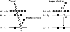
Figure 9: Schematic representation of Auger electron knockout by X-ray photons ($q^{2}=0$) or by virtual photons ($q^{2}\neq 0$) emitted by electrons irradiating the surface of a sample. In the first stage, the $K$ shell electron is excited to a continuum state (left panel). The resulting vacancy, $\gamma$, is filled with an electron from the $L_{1}$ shell ($\alpha$), which is accompanied by the radiation of a virtual photon to knock out an electron, $\beta$, from the $L_{2}$ or $L_{3}$ shell (right panel). The excitation energy $\varepsilon^{*}_{\gamma}$ goes to the formation of the vacancies $\alpha$ and $\beta$ and the kinetic energy $\varepsilon_{\mathrm{kin}}^{\mathrm{A}}$ of the Auger electron. By measuring the energy of the knocked-out electrons, it is possible to determine the peaks at energy values of the corresponding transitions.

Table 1: Total binding energies of neutral noble gas atoms in eVs. Column 2 shows our calculations using the Grasp2K package. The last three columns show the results of Lu et al. (1971); Desclaux (1973); Huang et al. (1976).

El	Grasp2K	Lu et al. (1971)	Desclaux (1973)	Huang et al. (1976)
Ne	3501.1	3472.0	3501.4	3500.8
Ar	14380.1	14072.6	14382.3	14382.1
Kr	75823.8	75739.0	75845.8	75851.7
Xe	202379.5	202402.7	202465.3	202498.4
Rn	640906.9	641899.1	641348.1	641591.6

The main question of interest is whether it is possible to calculate the two-hole excitation energy of atoms with an accuracy of 10 eV, which is attainable experimentally in Penning-trap mass spectrometry and is typical of the natural widths of two-hole excitations.

To estimate the magnitude of uncertainty, we first consider the total binding energy of inert gas atoms. Table 1 summarizes the results of our calculations performed using the Grasp2K software package. These results are compared to Lu et al. (1971), Desclaux (1973), and Huang et al. (1976). For light atoms, the variance is negligible. For the medium-heavy nucleus Xe, the variance does not exceed 120 eV. For Rn, the variance does not exceed 1 keV; the case of heavy atoms should be treated with caution.

Table 2: Single-electron ionization potentials for the noble gas series from Ne to Rn in eVs. The second and sixth columns list the hole quantum numbers: $n$ is the principal quantum number, $j$ is the total angular momentum, and $l$ is the orbital momentum. Columns 3 and 7 present results of our calculations using the Grasp2K package. Columns 4 and 8 list the results of Larkins (1977).

El	$n2jl$	Grasp2K	Larkins (1977)	El	$n2jl$	Grasp2K	Larkins (1977)
Ne	$110$	869.3	870.1		$310$	1151.4	1148.7
Ar	$110$	3205.8	3206.0		$311$	1005.5	1002.1
	$210$	327.0	326.3		$331$	943.3	940.6
	$211$	250.3	250.7		$410$	222.6	213.3
	$231$	248.2	248.6		$411$	169.2	145.5
Kr	$110$	14325.9	14325.6		$431$	156.8	145.5
	$210$	1930.7	1921.0	Rn	$110$	98390.5	98397.0
	$211$	1732.3	1727.2		$210$	18061.8	18048.0
	$231$	1679.3	1674.9		$211$	17335.6	17328.0
	$310$	295.9	292.1		$231$	14614.2	14610.0
	$311$	225.1	221.8		$310$	4489.7	4473.0
	$331$	217.0	214.5		$311$	4164.4	4150.0
Xe	$110$	34562.4	34564.4		$331$	3542.8	3529.0
	$210$	5458.8	5452.8		$410$	1104.9	1090.0
	$211$	5107.5	5103.7		$411$	961.3	944.0
	$231$	4786.9	4782.2		$431$	803.9	790.0

An estimate of the uncertainties in the energy of single-hole excitations can be obtained from Table 2, where the results of the Grasp2K package are compared with the data of Larkins (1977), obtained within the framework of a general semi-empirical method that takes into account experimental data on the binding energy of electron subshells and results of Hartree-Fock atomic calculations. For heavy atoms, the mismatch is basically on the order of 10 eV or less, and it is always less than 20 eV. The claimed accuracy of Larkins’ data is a few eVs for light atoms and 10 eV for heavy atoms.

The energies of two-hole excitations of the inert gas atoms of Ne and Ar are collected in Table 3; these data can further be supplemented with the results of calculating the energy of two-hole excitations of Kr, Xe and Rn. The results for $2\leq n_{\alpha}\leq 3$ and $2\leq n_{\beta}\leq 3$ are compared with the semi-empirical values extracted from the energy spectrum of Auger electrons Larkins (1977). The second column of these tables lists the total angular momentum $J$ of the two holes; then, the sums of the energies of the single-particle excitations and the energy of two-hole excitation, determined on the basis of Auger spectroscopy data, are presented. The next column, 5, reports two-hole excitation energy according to our calculations using the Grasp2K package. The last column contains quantum numbers of the pair $(n,2j,l)$. We remark that $n$ and $l$ are integers, $j$ are half-integers, and $2j$ are odd. Mixing occurs if some states of the pair arise in two or more combinations. The mixing matrix is presented in column 6. For mixed states, column 5 lists the energy eigenvalues. For example, for the Ar atom, the vacancies $|(210)(211)\rangle\equiv|2s_{1/2}2p_{1/2}\rangle$ and $|(210)(231)\rangle\equiv|2s_{1/2}2p_{3/2}\rangle$ with $J=1$ are mixed, whereby the eigenstates have the form

$$|J=1;~{}631.2~{}\mathrm{eV}\rangle = 0.612|(210)(211)\rangle+0.791|(210)(231)\rangle$$

$$|J=1;~{}606.8~{}\mathrm{eV}\rangle = 0.791|(210)(211)\rangle-0.612|(210)(231)\rangle.$$

The energy of these states are 631.2 eV and 606.8 eV, respectively. Larkins (1977) does not take into account such mixing. In the above example, the difference between the energies of the holes with and without the mixing is small. In the case of Xe, the deviation from the semi-empirical values of Larkins (1977) does not exceed 10 eV, whereas for Rn, the deviation does not exceed 40 eV. The deviation is negligible for light atoms.

Table 3: Double-electron ionization potentials for the noble gas atoms Ne and Ar in eVs. Column 2 lists the total angular momentum of the pair. Column 3 presents the sum of excitation energies of the single-hole states. The values of $\epsilon_{\alpha}^{*}$ and $\epsilon_{\beta}^{*}$ are from Larkins (1977). Column 4 reports the double-electron ionization potentials extracted from the Auger electrons spectroscopy data from Larkins (1977). The Auger transitions allow for the determination of the excitation energies of two-hole states with $n_{\alpha},n_{\beta}\geq 2$. Column 5 presents the results of our calculations using the Grasp2K package. The principal quantum number $n$, the total angular momentum $j$ and the orbital momentum $l$ of electron holes, $\alpha$ and $\beta$, are reported in the last columns. Column 6 presents the mixing matrix of two-hole states, which gives the energy eigenstates with definite $J$. The energy levels in columns 3 and 4 neglect mixing and are ordered in the coincidence with column 5, i.e., for a unit-mixing matrix.

El	$J$	$\epsilon_{\alpha}^{*}+\epsilon_{\beta}^{*}$	$\epsilon_{\alpha\beta}^{\mathrm{A}}$	$\epsilon_{\alpha\beta}^{*}$	$U(\cdot|\alpha\beta)$	$(n2jl)_{\alpha}\;(n2jl)_{\beta}$
Ne	0	1740.2		1862.1	1.000	$110\;110$
Ar	0	6412.0		6653.5	1.000	$110\;110$
	0	3532.3		3588.7	1.000	$110\;210$
	1	3532.3		3579.8	1.000	$110\;210$
	0	3456.7		3513.3	1.000	$110\;211$
	1	3456.7		3522.0	0.669  0.743	$110\;211$
		3454.6		3511.9	0.743 -0.669	$110\;231$
	2	3454.6		3510.1	1.000	$110\;231$
	0	652.6	695.4	695.0	1.000	$210\;210$
	0	577.0	606.7	607.6	1.000	$210\;211$
	1	577.0	630.0	631.2	0.612  0.791	$210\;211$
		574.9	605.9	606.8	0.791 -0.612	$210\;231$
	2	574.9	604.6	605.3	1.000	$210\;231$
	0	501.4	553.8	557.0	0.669  0.743	$211\;211$
		497.2	539.3	538.5	0.743 -0.669	$231\;231$
	1	499.3	538.9	538.0	1.000	$211\;231$
	2	499.3	545.8	545.1	0.881 -0.474	$211\;231$
		497.2	537.4	536.3	0.474  0.881	$231\;231$

The energies of the electron shells of noble gas atoms with double-$K$ holes are calculated by Niskanen et al. (2011). We obtain good agreement for Ne, Ar, Kr, and Xe, but the results are noticeably different for Rn. Niskanen et al. (2011) give $\epsilon_{{KK}}^{*}$ = 198912.6 eV, whereas our calculations yield the value of 198568.3 eV, which is 344 eV less. In the paper of Niskanen et al. (2011), QED corrections due to the electron self-energy and the vacuum polarization are not taken into account. If these effects are neglected in our calculations, then a value of 198977.8 eV is obtained; this value differs by only 65 eV from the result of Niskanen et al. (2011). The uncertainty in two-hole excitation energies of heavy atoms is thus found to be about 60 eV, which is higher than the $0\nu 2$EC target of 10 eV.

The $0\nu 2$EC half-lives are estimated in Sec. V and Sec. VIII by neglecting the mixing. The two-hole excitation energies of atoms with arbitrary $Z$ are determined using the data for Ne, Ar (Table 3), and also Kr, Xe and Rn by means of interpolation $\epsilon_{\alpha\beta}^{\ast}=aZ^{b}$ between the neighboring noble gas atoms with the same vacancies.

IV.3 Section summary

The probability of capture of orbital electrons by the nucleus depends on the value of the electron wave functions inside the nucleus. The values of upper and lower components of the Dirac electron wave functions of neutral atoms inside the nuclei are tabulated by Band and Trzhaskovskaya (1986), where the electron screening is accounted for using the relativistic Dirac-Fock-Slater and Dirac-Fock potentials. The $ns_{1/2}$ waves are dominant. The $np_{1/2}$ waves can be found to be enhanced compared to the $np_{3/2}$ waves. The nonrelativistic solutions of the $np_{3/2}$ waves are close to the relativistic ones (see also Grant (2007), Fig. 1.2). The electron capture from the $np_{3/2}$ orbits is therefore suppressed. The results of Band and Trzhaskovskaya (1986) are in good agreement with results provided by the Grasp2K software package.

The resonant enhancement of the $0\nu$2EC decays occurs when the excitation energies of the parent and intermediate daughter atoms are degenerate with an accuracy of about 10 eV. This scale characterizes the typical excitation width of the atomic shells. Accuracy of about 10 eV is achievable on Penning traps when measuring mass difference of ionized atoms. To identify the resonant $0\nu$2EC with the same high accuracy, information about double-hole excitations of electron shells is required.

The two-hole interactions provide a dominant contribution to the energy of excited electron shells but not the only contribution. Open vacancies in the occupation numbers affect the energy of all atomic levels. The Grasp2K package calculates the structure of electron shells based on the Green’s function method of QED, which offers a simple and clear description of various approximations.

Accuracy of up to 10 eV is readily achievable when determining theoretically single-hole excitation energies. We demonstrated independence on the gauge of single-hole excitation energies in the order $\alpha^{2}$Ry. One of the challenges of the atomic theory is the proof of gauge invariance of QED of multielectron atoms in all orders of perturbation theory. Double-hole excitation energies can be determined theoretically with an accuracy of 60 eV or better. The upper bound of the possible error is still higher than that required to identify the resonant $0\nu$2EC unambiguously. In calculations with atomic shell structure, the uncertainties are associated with complexity of the bound-state problem for multielectron atoms. In many cases, the resonant parameter of $0\nu$2EC can be extracted from the experimental data on Auger spectroscopy. When normalization to the experimental values is not possible, quantum chemistry codes such as Grasp2K can be used to get the missing information.

V Nuclear matrix elements

In this section we describe how nuclear structure affects the half-life of the $0\nu$2EC process and review the available calculations of the related NMEs. We also add new NME calculations in order to complement the list of the evaluated $0\nu$2EC cases.

V.1 Overview of the calculated nuclear matrix elements in 0$\nu$2EC

Nuclear structure is heavily involved in the decay amplitude (III.23) through the appropriate nuclear matrix elements (NMEs) Suhonen (2012a). These NMEs have been computed in various theory frameworks as described below. A representative list of the calculations is displayed in Table 4. In the table the available estimated lowest and highest limits for the near-resonant $0\nu 2$EC half-lives (last two columns) are listed. In the evaluation of the half-lives Eq. (VIII.1) was adopted and the NMEs $M^{0\nu}$ from column 4 of Table 4 were used, in addition to the degeneracy parameters taken from Tables 7 and 8. Also the theory frameworks used to derive these NMEs are given (column 5), along with the corresponding reference (column 6). The $Q_{\mathrm{2EC}}$-value measurements for the evaluation of the degeneracy parameters have been performed by the use of modern Penning-trap techniques (see Sec. VI).

In practically all the listed cases the decay rates are suppressed by the rather sizable magnitude of the ratio $(\Delta/\Gamma_{\alpha\beta})^{2}$, where $\Gamma_{\alpha\beta}\sim 10$ eV is the typical de-excitation width of the excited electron shells with the electron vacancies $\alpha$ and $\beta$. Decays to $0^{+}$ states are favored over the decays to $2^{+}$ or $1^{-},2^{-},3^{-}$ etc. states due to the involved nuclear wave functions and/or higher-order transitions. A further suppression stems from nuclear deformation. This suppression is typically a few tens of percent (Ejiri, 2019) but can be even stronger, factors of 2-3, for large deformations Delion and Suhonen (2017). The radial wave functions of electrons in low-lying atomic states on the surface of medium-heavy nuclei are from Band and Trzhaskovskaya (1986) . In relativistic theory, the electron capture from the $ns_{1/2}$ states is dominant, the amplitude of electron capture from the $np_{1/2}$ states is suppressed by about an order of magnitude, while the amplitude of electron capture from the $j\geq 3/2$ state appears to be suppressed by several orders of magnitude Kolhinen et al. (2010); Krivoruchenko et al. (2011).

There are some favorable values of degeneracy parameters listed in Table 8, like for the transitions ${}^{106}\textrm{Cd}\to\,^{106}\textrm{Pd}((2,3)^{-})$ and ${}^{156}\textrm{Dy}\to\,^{156}\textrm{Gd}(1^{-},2^{+})$ but the associated nuclear matrix elements are not yet evaluated. At the moment the most favorable case with a half-life estimate of $\gtrsim 5\times 10^{28}$ years is the case ${}^{152}\textrm{Gd}\to\,^{152}\textrm{Sm}(0^{+}_{\rm gs})$ which corresponds to a decay transition to the ground state.

All the presently identified favorable $0\nu$2EC cases are in the regions of relatively strong nuclear deformation so that a proper handling of this degree of freedom poses a challenge to the nuclear-theory frameworks.

V.2 Overview of the calculation frameworks

In the analyses of the near-resonant $0\nu 2$EC decay transitions the adopted many-body frameworks include the quasiparticle random-phase approximation (QRPA) in its higher-QRPA versions: multiple-commutator model (MCM), the deformed QRPA, the microscopic interacting boson model (IBM-2) and the energy-density functional (EDF) method. The MCM and deformed QRPA frameworks compute the $0\nu 2$EC-decay NME explicitly, including the contributions by the virtual states of the intermediate nucleus. The other two models, IBM-2 and EDF, resort to the closure approximation where the sum over the intermediate states, with the appropriate energy denominator, has been suppressed by assuming an average excitation energy in the denominator and then using the closure over the complete set of intermediate virtual states. All these models are briefly described below.

Table 4: The “sQRPA” and “dQRPA” of column 5 denote the spherical pnQRPA and deformed QRPA outlined in the beginning of Sec. V.B.1 and in Sec. V.B.2 , respectively. Furthermore, the symbol “IBM-2” denotes the microscopic interacting boson model of Sec. V.B.3 and the symbol “EDF” denotes the energy-density functional method of Sec. V.B.4. In the case of the multiple-commutator model (MCM of Sec. V.B.1) we have chosen to quote the results obtained by the use of the UCOM short-range correlations (UCOM s.r.c.) which are the very realistic ones Kortelainen et al. (2007). The UCOM s.r.c. have also been used in the sQRPA, dQRPA and EDF calculations. The “qp estimate” in the fifth column denotes the procedure outlined in Sec. V.C. The last two columns give the minimum and maximum half-lives (in years) calculated using Eq. (VIII.1) with $K_{Z}$ of Eq. (III.21), $m_{\beta\beta}=100$ meV and $g_{A}=1.27$. The excitation energies are given in keV.

Transition	$J^{\pi}_{f}$	$M^{*}_{A,Z-2}-M_{A,Z-2}$	$M^{0\nu}$	Model	Ref.	$T_{1/2}^{\min}$	$T_{1/2}^{\max}$
${}^{\;\,74}_{\;\,34}$Se$\to^{\;\,74}_{\;\,32}$Ge∗∗	2${}^{+}_{2}$	$1204.205\pm 0.007$	$3.22\times 10^{-4}$	MCM	Kolhinen et al. (2010)	$1.2\times 10^{46}$	$1.2\times 10^{46}$
${}^{\;\,96}_{\;\,44}$Ru$\to^{\;\,96}_{\;\,42}$Mo∗∗	[0+]	$2712.68\pm 0.10$	5.57	MCM	Suhonen (2012b)	$2.2\times 10^{32}$	$6.8\times 10^{32}$
${}^{106}_{\;\,48}$Cd$\to^{106}_{\;\,44}$Pd∗∗	[0+]	$2717.59\pm 0.21$	3.38 - 3.48	MCM	Suhonen (2011)	$5.3\times 10^{31}$	$7.0\times 10^{31}$
${}^{112}_{~{}50}$Sn$\to^{112}_{~{}48}$Cd∗∗	(0+)	$2988\pm 8$	4.76	estimate	Rahaman et al. (2009)	$3.5\times 10^{35}$	$3.8\times 10^{35}$
${}^{124}_{\;\,54}$Xe$\to^{124}_{\;\,52}$Te∗∗	0${}^{+}_{4}$	$2153.29\pm 0.03$	1.11 - 1.30	MCM	Suhonen (2013)	$7.3\times 10^{35}$	$7.3\times 10^{35}$
			0.297	IBM-2	Kotila et al. (2014)	$1.2\times 10^{37}$	$1.2\times 10^{37}$
${}^{136}_{\;\,58}$Ce$\to^{136}_{\;\,56}$Ba∗∗	0${}^{+}_{4}$	$2315.32\pm 0.07$	0.68	MCM	Kolhinen et al. (2011)	$3.3\times 10^{32}$	$4.3\times 10^{32}$
${}^{152}_{\;\,64}$Gd$\to^{152}_{\;\,62}$Sm∗	0${}^{+}_{1}$	0	7.21 - 7.59	sQRPA	Šimkovic et al. (2011)	$6.8\times 10^{27}$	$6.8\times 10^{28}$
			2.67 - 3.23	dQRPA	Fang et al. (2012)	$4.3\times 10^{28}$	$4.3\times 10^{29}$
			2.445	IBM-2	Kotila et al. (2014)	$6.0\times 10^{28}$	$6.0\times 10^{29}$
			0.89 - 1.07	EDF	Rodríguez and Martínez-Pinedo (2010)	$3.8\times 10^{29}$	$3.8\times 10^{30}$
${}^{156}_{\;\,66}$Dy$\to^{156}_{\;\,64}$Gd∗∗	0${}^{+}_{1}$	0	3.175	IBM-2	Kotila et al. (2014)	$7.3\times 10^{34}$	$7.3\times 10^{34}$
	0${}^{+}_{2}$	$1049.487\pm 0.002$	1.749	IBM-2	Kotila et al. (2014)	$4.8\times 10^{34}$	$4.8\times 10^{34}$
	0${}^{+}_{3}$	$1168.186\pm 0.007$	0.466	IBM-2	Kotila et al. (2014)	$5.0\times 10^{35}$	$5.0\times 10^{35}$
	0${}^{+}_{4}$	$1715.192\pm 0.005$	0.311	IBM-2	Kotila et al. (2014)	$7.5\times 10^{34}$	$7.5\times 10^{34}$
	0${}^{+}_{5}$	$1851.239\pm 0.007$	0.346	IBM-2	Kotila et al. (2014)	$4.8\times 10^{33}$	$4.8\times 10^{33}$
	0${}^{+}_{6}$	$1988.5\pm 0.2$	0.3	estimate	This work	$1.1\times 10^{28}$	$9.5\times 10^{32}$
${}^{164}_{\;\,68}$Er$\to^{164}_{\;\,66}$Dy∗	0${}^{+}_{1}$	0	5.94 - 6.12	sQRPA	Šimkovic et al. (2011)	$3.3\times 10^{31}$	$3.5\times 10^{31}$
			2.27 - 2.64	dQRPA	Fang et al. (2012)	$2.0\times 10^{32}$	$2.1\times 10^{32}$
			3.952	IBM-2	Kotila et al. (2014)	$7.8\times 10^{31}$	$8.0\times 10^{31}$
			0.50 - 0.64	EDF	Rodríguez and Martínez-Pinedo (2010)	$3.8\times 10^{33}$	$4.0\times 10^{33}$
${}^{180}_{\;\,74}$W$\to^{180}_{\;\,72}$Hf∗	0${}^{+}_{1}$	0	5.56 - 5.79	sQRPA	Šimkovic et al. (2011)	$1.4\times 10^{29}$	$1.8\times 10^{29}$
			1.79 - 2.05	dQRPA	Fang et al. (2012)	$1.2\times 10^{30}$	$1.6\times 10^{30}$
			4.672	IBM-2	Kotila et al. (2014)	$2.1\times 10^{29}$	$2.8\times 10^{29}$
			0.38 - 0.58	EDF	Rodríguez and Martínez-Pinedo (2010)	$2.0\times 10^{31}$	$2.5\times 10^{31}$
${}^{184}_{\;\,76}$Os$\to^{184}_{\;\,74}$W∗∗	0${}^{+}_{2}$	$1002.48\pm 0.04$	0.631	EDF	Smorra et al. (2012)	$6.8\times 10^{33}$	$6.8\times 10^{33}$
	(0)${}^{+}_{3}$	$1322.152\pm 0.022$	0.504	EDF	Smorra et al. (2012)	$6.0\times 10^{30}$	$1.2\times 10^{31}$
	2${}^{+}_{5}$	$1431.02\pm 0.05$	0.14	MCM	This work	$4.5\times 10^{32}$	$4.5\times 10^{37}$
	(0)${}^{+}_{5}$	$1713.47\pm 0.10$	0.163	EDF	Smorra et al. (2012)	$1.7\times 10^{35}$	$1.7\times 10^{35}$
${}^{190}_{\;\,76}$Pt$\to^{190}_{\;\,74}$Os∗∗	1+	$1326.9\pm 0.5$	1.1	MCM	This work	$3.3\times 10^{26}$	$1.6\times 10^{30}$
	$(0_{3})^{+}$	$1382.4\pm 0.2$	4.7	MCM	This work	$1.0\times 10^{30}$	$6.5\times 10^{30}$
${}^{148}_{\;\,64}$Gd$\to^{148}_{\;\,62}$Sm∗∗	[0+]	$3004\pm 3$	0.071	qp estimate	This work	$5.3\times 10^{28}$	$1.5\times 10^{35}$
	[1+]		0.031	qp estimate	This work	$8.3\times 10^{28}$	$2.5\times 10^{35}$
${}^{150}_{\;\,64}$Gd$\to^{150}_{\;\,62}$Sm∗∗	0+	$1255.400\pm 0.022$	0.066	qp estimate	This work	$4.0\times 10^{29}$	$1.6\times 10^{36}$
${}^{154}_{\;\,66}$Dy$\to^{154}_{\;\,64}$Gd∗∗	[0+]	$3153.1$	0.068	qp estimate	This work	$6.8\times 10^{34}$	$2.8\times 10^{35}$
	[0+]	$3154.8\pm 0.4$	0.068	qp estimate	This work	$6.3\times 10^{34}$	$2.8\times 10^{35}$
	(1+)	$3264.42\pm 0.21$	0.030	qp estimate	This work	$7.5\times 10^{28}$	$3.8\times 10^{35}$
${}^{194}_{\;\,80}$Hg$\to^{194}_{\;\,78}$Pt∗∗	(0+)	$2450\pm 5$	0.017	qp estimate	This work	$2.5\times 10^{29}$	$1.2\times 10^{36}$
	(1+)		0.004	qp estimate	This work	$1.4\times 10^{30}$	$6.3\times 10^{36}$
	(0+)	$2472\pm 5$	0.017	qp estimate	This work	$2.5\times 10^{29}$	$1.2\times 10^{36}$
	(1+)		0.004	qp estimate	This work	$1.4\times 10^{30}$	$2.8\times 10^{36}$
	[1+]	$2500\pm 10$	0.004	qp estimate	This work	$1.4\times 10^{30}$	$6.5\times 10^{36}$
${}^{202}_{\;\,82}$Pb$\to^{202}_{\;\,78}$Hg∗∗	0${}^{+}_{2}$	$1411.37\pm 0.12$	0.011	qp estimate	This work	$1.7\times 10^{30}$	$1.6\times 10^{37}$
	(1${}^{+})$	$1347.92\pm 0.07$	0.003	qp estimate	This work	$4.0\times 10^{33}$	$4.8\times 10^{36}$

The NME for the near-resonant $0\nu 2$EC decay to the $0^{+}$ final states is written as a linear combination of the Gamow-Teller (GT), Fermi (F) and tensor (T) NMEs as

$$M^{\rm 2EC}=M_{\rm GT}^{\rm 2EC}-\left(\frac{g_{\rm V}}{g_{\rm A}}\right)^{2}M_{\rm F}^{\rm 2EC}+M_{\rm T}^{\rm 2EC}\,.$$ (V.1)

In the MCM and deformed QRPA frameworks the transitions through the virtual states of the intermediate nucleus are treated explicitly. Then the double Fermi, Gamow–Teller, and tensor nuclear matrix elements can be written as

$$M_{\rm F}^{\rm 2EC} =\sum_{k}(J^{+}_{f}||\sum_{mn}h_{\rm F}(r_{mn},E_{k})||0^{+}_{i})\,,$$ (V.2)

$$M_{\rm GT}^{\rm 2EC} =\sum_{k}(J^{+}_{f}||\sum_{mn}h_{\rm GT}(r_{mn},E_{k})(\mbox{\boldmath{$\sigma$}}_{m}\cdot\mbox{\boldmath{$\sigma$}}_{n})||0^{+}_{i})\,,$$ (V.3)

$$M_{\rm T}^{\rm 2EC} =\sum_{k}(J^{+}_{f}||\sum_{mn}h_{\rm T}(r_{mn},E_{k})S^{\rm T}_{mn}||0^{+}_{i})\,,$$ (V.4)

where the tensor operator reads

$$S^{\rm T}_{mn}=3[(\mbox{\boldmath{$\sigma$}}_{m}\cdot\hat{\mathbf{r}}_{mn})(\mbox{\boldmath{$\sigma$}}_{n}\cdot\hat{\mathbf{r}}_{mn})]-\mbox{\boldmath{$\sigma$}}_{m}\cdot\mbox{\boldmath{$\sigma$}}_{n}\,.$$ (V.5)

The summations over $k$ in Eqs. (V.2), (V.3) and (V.4) run over all the states of the intermediate odd-odd nucleus, $r_{mn}=|\mathbf{r}_{m}-\mathbf{r}_{n}|$ is the relative distance between the two decaying protons, labeled $m$ and $n$, and $\hat{\mathbf{r}}_{mn}=(\mathbf{r}_{m}-\mathbf{r}_{n})/r_{mn}$. The neutrino potentials $h_{\rm K}(r_{mn},E_{k})$, $K=\textrm{F,~{}GT,~{}T}$, are given by Suhonen (2012a). The ground state of the initial even-even nucleus is denoted by $0^{+}_{i}$ and the positive-parity final state in the daughter even-even nucleus is denoted by $J^{+}_{f}$. In the closure approximation the intermediate energies $E_{k}$ in the above equations are replaced by one single energy $E$ and the summation over $k$ is replaced by a unit operator.

In general, for the near-resonant $0\nu 2$EC decay to the final $J^{+}_{f}=0^{+},1^{+},2^{+}$ states the NMEs can be written in the QRPA framework in the form

$$M_{K}^{\rm 2EC}(0^{+}_{i}\to J_{f}^{+}) =(-1)^{J_{f}}\sum_{J^{\pi},k_{1},k_{2}}\sum_{J_{1},J^{\prime},J^{\prime\prime}}\sum_{pp^{\prime}nn^{\prime}}\sqrt{\frac{[J^{\prime}][J^{\prime\prime}][J_{1}]}{[J_{f}]}}$$

$$\times\left\{\begin{array}[]{ccc}j_{n}&j_{p}&J\\ j_{n^{\prime}}&j_{p^{\prime}}&J_{1}\\ J^{\prime\prime}&J^{\prime}&J_{f}\end{array}\right\}(nn^{\prime}:J^{\prime\prime}||{\mathcal{O}}_{K}^{(J_{f})}||pp^{\prime}:J^{\prime})$$ (V.9)

$$\times(J^{+}_{f}||\big{[}c^{{\dagger}}_{n^{\prime}}\tilde{c}_{p^{\prime}}\big{]}_{J_{1}}||J^{\pi}_{k_{1}})\langle J^{\pi}_{k_{1}}|J^{\pi}_{k_{2}}\rangle(J^{\pi}_{k_{2}}||\big{[}c^{{\dagger}}_{n}\tilde{c}_{p}\big{]}_{J}||0^{+}_{i})\,,$$

where $[x]=2x+1$ and $k_{1}$ and $k_{2}$ label the different QRPA solutions for a given multipole $J^{\pi}$, stemming from the parent and daughter nuclei of the near-resonant $0\nu 2$EC decay. The operators ${\mathcal{O}}_{K}^{(0_{f})}$ for the $0^{+}$ final states in the reduced two-particle matrix element denote the Fermi (K=F), Gamow-Teller (K=GT) and tensor (K=T) parts of the double-beta operator, given in Eqs. (V.2)–(V.4). In all the discussed theory frameworks the two-particle matrix element contains also the appropriate short-range correlations, higher-order nucleonic weak currents and nucleon form factors, as given by Šimkovic et al. (1999). The last line of Eq. (V.2) contains the one-body transition densities between the initial/final ground state ($0^{+}_{i}$/$0^{+}_{f}$) and the intermediate states $J^{\pi}_{k}$, and they can be obtained in the QRPA framework as discussed below. The term between the one-body transition densities is the overlap between the two sets of intermediate states emerging from the two QRPA calculations based on the parent and daughter even-even ground states and its expression for the spherical nuclei has been given by Suhonen (2012a) and for deformed nuclei by Šimkovic et al. (2004).

Here it should be noted that typically only the $J_{f}^{+}=0^{+}$ final states have been considered in the near-resonant $0\nu 2$EC-decay calculations, as given by Eqs. (V.2) - (V.4) and the $J_{f}=0$ special case of Eq. (V.2). The simplest procedure to reach the positive-parity $J_{f}^{+}=1^{+},2^{+}$ states is to use a generalized GT-type of operator:

$$M_{\rm GT}^{\rm 2EC}(J_{f}^{+}=1^{+},2^{+})=\sum_{k}(J_{f}^{+}||\sum_{mn}h_{\rm GT}(r_{mn},E_{k})\big{[}\mbox{\boldmath{$\sigma$}}_{m}\mbox{\boldmath{$\sigma$}}_{n}\big{]}_{J_{f}}||0^{+}_{i})\,,$$ (V.10)

together with the expression (V.2). In Sec. V.3 we compute this NME for several cases of interest in an approximate way avoiding the vast complications involved in the use of detailed nuclear wave functions for high-excited states in heavy daughter nuclei of the near-resonant $0\nu 2$EC processes. Furthermore, to reach the negative-parity states $J_{f}^{-}=0^{-},1^{-},2^{-}$ one would need more complex nuclear transition operators and these are not thoroughly examined yet Vergados (2011). In this work we then skip the estimation of the order of magnitude of the related NMEs.

Here it has to be remarked that in the very recent studies Cirigliano et al. (2018c) and Cirigliano et al. (2019) it was found that in addition to the long-range NME V.1 there is a notable contribution from a short-range operator affecting the Fermi part of the NME. According to preliminary studies in these works for very light nuclei the value of the NME of the neutrinoless double beta decay could change considerably by the inclusion of the new short-range term. It remains to be seen how strong is the effect for the medium-heavy and heavy nuclei which actually double beta decay.

V.2.1 Multiple-commutator model

The nuclear states of odd-odd nuclei can be described within the spherical proton-neutron quasiparticle random-phase approximation (pnQRPA) framework. The solution of the pnQRPA equations can be written as (see, e.g. Suhonen (2007))

$$|\omega\,M\rangle =q^{\dagger}(\omega,M)|\textrm{QRPA}\rangle$$

$$=\sum_{pn}\left(X_{pn}^{\omega}\left[a_{p}^{\dagger}a_{n}^{\dagger}\right]_{JM}-Y_{pn}^{\omega}\left[a_{p}^{\dagger}a_{n}^{\dagger}\right]_{JM}^{\dagger}\right)|\textrm{QRPA}\rangle\,,$$ (V.11)

where the shorthand $\omega=J^{\pi}_{k}$ for the $k^{th}$ intermediate state of spin-parity $J^{\pi}$ has been used. Here $|\textrm{QRPA}\rangle$ is the QRPA ground state and the operator $a_{p}^{\dagger}$ creates a proton quasiparticle on the single-particle orbital $p=(n_{p},l_{p},j_{p})$, where $n$ is the principal, $l$ the orbital angular-momentum and $j$ the total angular-momentum quantum number. The operator $a_{p}$ is the corresponding annihilation operator and a similar definition applies for the neutrons $n$. The single-particle orbitals are obtained by solving the Schrödinger equation for a spherical Woods-Saxon mean-field potential Suhonen (2007). By using this wave function one can obtain the transition densities

$$(0^{+}_{\rm gs}||[c^{{\dagger}}_{n^{\prime}}\tilde{c}_{p^{\prime}}]_{J}||J^{\pi}_{k_{1}}) =\sqrt{[J]}\left[v_{n^{\prime}}u_{p^{\prime}}X^{J^{\pi}k_{1}}_{p^{\prime}n^{\prime}}+u_{n^{\prime}}v_{p^{\prime}}Y^{J^{\pi}k_{1}}_{p^{\prime}n^{\prime}}\right]\ ,$$ (V.12)

$$(J^{\pi}_{k_{2}}||[c^{{\dagger}}_{n}\tilde{c}_{p}]_{J}||0^{+}_{i}) =\sqrt{[J]}\left[\tilde{u}_{n}\tilde{v}_{p}\tilde{X}^{J^{\pi}k_{2}}_{pn}+\tilde{v}_{n}\tilde{u}_{p}\tilde{Y}^{J^{\pi}k_{2}}_{pn}\right]\,,$$ (V.13)

where $v$ ($\tilde{v}$) and $u$ ($\tilde{u}$) correspond to the BCS occupation and vacancy amplitudes of the final (initial) even-even nucleus. The amplitudes $X$ and $Y$ ($\tilde{X}$ and $\tilde{Y}$) come from the pnQRPA calculation starting from the final (initial) nucleus of the double-beta decay. Here the initial and final states of the near-resonant $0\nu 2$EC decay are assumed to be the ground states of the even-even mother and daughter nuclei.

The $n^{th}$ excited $\omega_{f}=I^{\pi}_{n}$ state, where $I$ is the angular momentum of the state, in the even-even daughter nucleus is described in the QRPA formalism, and the corresponding wave function can be presented as (see Suhonen (2007))

$$|I^{\pi}_{n}\,M_{I}\rangle =Q^{\dagger}(I^{\pi}_{n},M_{I})|\textrm{QRPA}\rangle$$

$$=\sum_{a\leq b}\big{[}X_{ab}^{\omega_{f}}A^{\dagger}_{ab}(IM_{I})-Y_{ab}^{\omega_{f}}\tilde{A}_{ab}(IM_{I})\big{]}|\textrm{QRPA}\rangle\,,$$ (V.14)

where the normalized two-quasiparticle operators are defined as

$$A^{\dagger}_{ab}(IM_{I})=\mathcal{N}_{ab}(I)\left[a^{\dagger}_{a}a^{\dagger}_{b}\right]_{IM_{I}}\,,$$ (V.15)

$$\mathcal{N}_{ab}(I)=\frac{\sqrt{1+\delta_{ab}(-1)^{I}}}{1+\delta_{ab}}$$ (V.16)

for any state of angular momentum $I$ in the even-even nucleus. We denote here $\tilde{A}_{ab}(IM_{I})\equiv(-1)^{I+M_{I}}A_{ab}(I,-M_{I})$. Here $a$ and $b$ denote the quantum numbers of a single-particle orbital in a spherical nuclear mean field, including the number of nodes $n$ (principal quantum number), the orbital ($l$) and total ($j$) angular momenta. It should be noted that here the summation over $a\leq b$ guarantees that there is no double counting of two-quasiparticle configurations and this with the normalized operators (V.15) guarantees that the wave function is properly normalized with the normalization condition Suhonen (2007)

$$\sum_{a\leq b}\Big{(}\big{|}X_{ab}^{\omega_{f}}\big{|}^{2}-\big{|}Y_{ab}^{\omega_{f}}\big{|}^{2}\Big{)}=1\,.$$ (V.17)

The creation operator $Q^{\dagger}(I^{\pi}_{n},M_{I})$ of (V.2.1) is usually called the creation operator for a QRPA phonon.

For calculational convenience it is preferable to go from the restricted sum of (V.2.1) to a non-restricted (free) one by introducing the correspondence

$$|I^{\pi}_{n}\,M_{I}\rangle=\bar{Q}^{\dagger}(I^{\pi}_{n},M_{I})|\textrm{QRPA}\rangle$$

$$=\sum_{ab}\big{[}\bar{X}_{ab}^{\omega_{f}}\bar{A}^{\dagger}_{ab}(IM_{I})-\bar{Y}_{ab}^{\omega_{f}}\tilde{\bar{A}}_{ab}(IM_{I})\big{]}|\textrm{QRPA}\rangle\,,$$ (V.18)

where the barred two-quasiparticle operators are the ones of (V.15) without the normalizer $\mathcal{N}_{ab}(I)$. Then the normalization condition becomes

$$\sum_{ab}\Big{(}\big{|}\bar{X}_{ab}^{\omega_{f}}\big{|}^{2}-\big{|}\bar{Y}_{ab}^{\omega_{f}}\big{|}^{2}\Big{)}=\frac{1}{2}\,.$$ (V.19)

At the same time the two kinds of $X$ and $Y$ amplitudes are related by

$$\bar{X}_{ab}^{\omega_{f}}=\frac{\sqrt{1+\delta_{ab}}}{2}X_{ab}^{\omega_{f}}\ ;\ \bar{Y}_{ab}^{\omega_{f}}=\frac{\sqrt{1+\delta_{ab}}}{2}Y_{ab}^{\omega_{f}}\,,\ a\leq b\,,$$ (V.20)

for any $\omega_{f}=I^{\pi}_{n}$. The barred amplitudes are symmetrized ones and possess the convenient symmetry relations (to generate amplitudes with $a>b$):

$$\bar{X}_{ba}^{\omega_{f}}=(-1)^{j_{a}+j_{b}+J+1}\bar{X}_{ab}^{\omega_{f}}\ ;\ \bar{Y}_{ba}^{\omega_{f}}=(-1)^{j_{a}+j_{b}+J+1}\bar{Y}_{ab}^{\omega_{f}}\,.$$ (V.21)

In the MCM, originally introduced in Suhonen (1993), the one-body transition densities corresponding to a transition from the intermediate $|\omega\,M\rangle$ state (V.2.1) of the odd-odd nucleus to the final one-phonon state (V.2.1) of the even-even daughter nucleus are calculated by first writing the transition densities as ground-state-averaged multiple commutators and then applying the quasi-boson approximation Suhonen (2007) by replacing the QRPA vacuum by the BCS vacuum when taking the ground-state average. The averaged multiple commutators then become

$$\langle\omega_{f}\,M_{I}|\beta^{+}_{L\mu}(np)|\omega\,M\rangle$$

$$\approx\langle\textrm{BCS}|\big{[}[\bar{Q}(\omega_{f},M_{I}),\beta^{+}_{L\mu}(np)],q^{\dagger}(\omega,M)\big{]}|\textrm{BCS}\rangle\,,$$ (V.22)

where $|\textrm{BCS}\rangle$ is the BCS ground state and we have denoted the $\beta^{+}$ type of EC operator by

$$\beta^{+}_{L\mu}(np)\equiv\left[c^{\dagger}_{n}\tilde{c}_{p}\right]_{L\mu}\,,$$ (V.23)

with $c^{\dagger}_{n}$ creating a neutron on orbital $n$ and $\tilde{c}_{p}$ annihilating a proton on orbital $p$. Using the Wigner-Eckart theorem Suhonen (2007) one can convert (V.2.1) to the reduced transition density:

$$(\omega_{f}||\left[c^{\dagger}_{n}\tilde{c}_{p}\right]_{L}||\omega)=2\sqrt{[I][L][J]}(-1)^{I+L}$$

$$\times\sum_{n^{\prime}}(-1)^{j_{p}+j_{n^{\prime}}}\Big{(}\bar{X}^{\omega_{f}}_{n^{\prime}n}X^{\omega}_{n^{\prime}p}u_{n}u_{p}-\bar{Y}^{\omega_{f}}_{n^{\prime}n}Y^{\omega}_{n^{\prime}p}v_{n}v_{p}\Big{)}\left\{\begin{array}[]{ccc}J&L&I\\ j_{n}&j_{n^{\prime}}&j_{p}\end{array}\right\}$$ (V.26)

$$+2\sqrt{[I][L][J]}(-1)^{I+J}$$

$$\times\sum_{p^{\prime}}(-1)^{j_{n}+j_{p}}\Big{(}-\bar{X}^{\omega_{f}}_{p^{\prime}p}X^{\omega}_{np^{\prime}}v_{n}v_{p}+\bar{Y}^{\omega_{f}}_{p^{\prime}p}Y^{\omega}_{np^{\prime}}u_{n}u_{p}\Big{)}\left\{\begin{array}[]{ccc}J&L&I\\ j_{p}&j_{p^{\prime}}&j_{n}\end{array}\right\}\,,$$ (V.29)

where the $v$ and $u$ factors are the occupation and vacancy amplitudes of the BCS Suhonen (2007). The transition density (V.2.1) can be used to compute the connection of the near-resonant $0\nu 2$EC intermediate states to the final resonant excited state $\omega_{f}$ of Eq. (V.2.1).

The MCM method has close connection with the boson-expansion method described in the papers of Raduta et al. (1991b, a); Raduta and Suhonen (1996).

V.2.2 Deformed quasiparticle random phase approximation

The near-resonant $0\nu 2$EC NMEs for axially symmetric well-deformed nuclei can be calculated in the adiabatic Bohr-Mottelson approximation in the intrinsic coordinate system of a rotating nucleus. The nuclear excitations are characterized by the parity $\pi$ and the quantum number $K$ which is associated to the projection of the total angular momentum $J$ of the nucleus onto the intrinsic symmetry axis. Then the $k^{th}$ intrinsic state of projection-parity $K^{\pi}$, $|K^{\pi},\,k\rangle$, can be generated by the deformed QRPA approach Fang et al. (2011) in a way analogous to Eq. (V.2.1):

$$|K^{\pi}\,k\rangle =q^{\dagger}(K^{\pi},k)|0^{+}_{\rm gs}\rangle$$

$$=\sum_{pn}\left(X_{pn,K}^{k}a_{p}^{\dagger}a_{\bar{n}}^{\dagger}-Y_{pn,K}^{k}a_{\bar{p}}a_{n}\right)|0^{+}_{\rm gs}\rangle\,,$$ (V.30)

where for the quasiparticle operators $a_{\bar{p}}$ ($a_{\bar{n}}$) the $\bar{p}$ ($\bar{n}$) denotes the time-reversed proton (neutron) orbital. The quasiparticle pairs in (V.2.2) obey the selection rules $\Omega_{p}-\Omega_{n}=K$ and $\pi_{p}\pi_{n}=\pi$, where the involved parities are those of the single-particle orbitals and $\Omega$ denotes the projection of the total single-particle angular momentum $j$ on the intrinsic symmetry axis. The state $|0^{+}_{\rm gs}\rangle$ denotes here the vacuum of the deformed QRPA. The single-particle states are obtained by solving the Schrödinger equation for a deformed axially symmetric Woods-Saxon mean-field potential Yousef et al. (2009). In the deformed QRPA approach the deformed calculation is transformed to a spherical QRPA framework by decomposing the deformed Woods-Saxon wave functions first into deformed harmonic-oscillator (HO) wave functions and these, in turn, into spherical HO wave functions Yousef et al. (2009). This also enables the use of realistic one-boson-exchange nucleon-nucleon potentials in the many-body calculations Yousef et al. (2009).

The one-body transition densities (V.12) and (V.13) of the spherical QRPA are now replaced by the corresponding transition densities of the deformed QRPA:

$$\langle 0^{+}_{\rm gs}|c^{{\dagger}}_{n^{\prime}}c_{p^{\prime}}]_{J}|K^{\pi}\,k_{1}\rangle =v_{n^{\prime}}u_{p^{\prime}}X^{k_{1}}_{p^{\prime}n^{\prime},K^{\pi}}+u_{n^{\prime}}v_{p^{\prime}}Y^{k_{1}}_{p^{\prime}n^{\prime},K^{\pi}}\ ,$$ (V.31)

$$\langle K^{\pi}\,k_{2}|c^{{\dagger}}_{n}\tilde{c}_{p}|0^{+}_{i}\rangle =\tilde{u}_{n}\tilde{v}_{p}\tilde{X}^{k_{2}}_{pn,K^{\pi}}+\tilde{v}_{n}\tilde{u}_{p}\tilde{Y}^{k_{2}}_{pn,K^{\pi}}\,.$$ (V.32)

These transition densities are the ones used to compute the near-resonant $0\nu 2$EC NMEs of the decays of ¹⁵²Gd, ¹⁶⁴Er and ¹⁸⁰W in the paper of Fang et al. (2012).

V.2.3 Microscopic interacting boson model

The interacting boson model (IBM) is a theory framework based on $s$ and $d$ bosons which correspond to collective nucleon pairs coupled to angular momenta and parities $0^{+}$ and $2^{+}$, respectively. An extension of the IBM is the microscopic IBM (IBM-2) where the protons and neutrons form separate proton and neutron bosons. The IBM-2 is in a way a phenomenological version of the nuclear shell model, containing the seniority aspect and the restriction to one magic shell in terms of the single-particle model space. The Hamiltonian and the transition operators are constructed from the $s$ and $d$ bosons as lowest-order boson expansions with coupling coefficients to be determined by fits to experimental data on low-lying energy levels and E2 $\gamma$ transitions associated with the $s$ and $d$ bosons, but the fitting does not use the spin or isovector data available from e.g. the $\beta$ decays. One can also relate the bosons to the underlying fermion model space through a mapping procedure Otsuka et al. (1978); Otsuka (1996).

The microscopic IBM can be extended to include higher-multipole bosons, like $g$ bosons, as well. Further extension concerns the description of odd-$A$ nuclei by the use of the microscopic interacting boson-fermion model (IBFM-2) Iachello and Isacker (1991). The IBM concept can also be used to describe odd-odd nuclei by using the interacting boson-fermion-fermion model (IBFFM) and its proton-neutron variant, the proton-neutron IBFFM (IBFFM-2) Brant and Paar (1988). Here problems arise from the interactions between the bosons and the one or two extra fermions in the Hamiltonian, and from the transition operators containing a large number of phenomenological parameters to be determined in some meaningful way. While IBM-2 has been used quite much to calculate the $0\nu 2\beta$ properties of nuclei the IBFFM-2 has not. The IBM-2 calculations have to be done using the closure approximation since it does not contain the spin-isospin degree of freedom needed to access the intermediate odd-odd nucleus of the $0\nu 2\beta$ decay, in particular in the context of the near-resonant $0\nu 2$EC decays.

V.2.4 Energy-density functional method

The energy-density functional method (EDF) is a mean-field-based method that uses closure approximation to compute the near-resonant $0\nu 2$EC NMEs, and thus is well suited for $0\nu 2$EC transitions between two ground states, like in the cases of the near-resonant $0\nu 2$EC decays of ¹⁵²Gd, ¹⁶⁴Er and ¹⁸⁰W treated in the paper of Rodríguez and Martínez-Pinedo (2012). In this theory framework Rodríguez and Martínez-Pinedo (2010) density functionals based on the Gogny D1S functional Berger et al. (1984) and D1M Goriely et al. (2009) in large single-particle bases (11 major oscillator shells) are used. Both the particle-number and angular-momentum projections are performed before the variation for the mother and daughter nuclei, and configuration mixing is taken into account using the generating coordinate method (GCM) Ring and Schuck (1980). Hence, in the EDF the initial and final ground states can be written as

$$|0^{+}_{\rm gs}\rangle=\sum_{\beta_{2}}g_{\beta_{2}}P^{J=0}P^{N}P^{Z}|\Phi_{\beta_{2}}\rangle\,,$$ (V.33)

where $P^{N}$ ($P^{Z}$) is the projection operator for a given neutron (proton) number and $P^{J=0}$ is the projection operator for zero total angular momentum. The intrinsic axially symmetric Hartree-Fock-Bogoliubov wave functions $|\Phi_{\beta_{2}}\rangle$ are solutions to the variation equations after particle-number-projection constrained to a given value of the axial quadrupole deformation $\beta_{2}$. The shape-mixing coefficients $g_{\beta_{2}}$ are found by solving the Hill-Wheeler-Griffin equation Ring and Schuck (1980).

V.3 Decays of nuclides with the calculated nuclear matrix elements

The order of magnitude of the NME (V.10) can be estimated by constructing a generic single-quasiparticle type NME (qp-NME) describing the conversion of a proton pair to a neutron pair at the nuclear proton and neutron Fermi surfaces. This NME picks the essential features of the transition since the most action is concentrated at the Fermi surfaces. The detailed quasiparticle properties at the Fermi surfaces can be obtained from a BCS calculation using the Woods-Saxon mean-field single-particle energies Bohr and Mottelson (1969). In this simple estimation the collective effects are not taken into account. These collective effects can be very important for $0\nu 2$EC transitions to the lowest-lying $0^{+}$ or $2^{+}$ states. However, for the $J_{f}=0^{+},2^{+}$ states at energies satisfying the resonance condition of the near-resonant $0\nu 2$EC decay the collective effects are not so important. In fact, at around these energies the many-body wave functions can vary strongly from one state to the next, sometimes causing coherent enhancements or incoherent cancellations. A qp-NME is a kind of average between these two extremes and thus suitable for the role of a generic NME in this case.

A plausible simplification of the NME (V.2) is to consider the conversion of an angular-momentum-zero-coupled proton pair to an angular-momentum-$J_{f}$-coupled neutron pair at the nuclear Fermi surface. The zero-coupled proton pairs are the most important contributors to the NMEs of the ordinary 0$\nu$2$\beta$ decay Hyvärinen and Suhonen (2015), so that this is a good simplifying approximation. Considering the $1^{+}$ type of intermediate states as the typical ones and taking $J_{1}=1$ for simplicity, leads to the following simplified expression for the NME (V.2):

$$M_{K}^{\rm 2EC}(0^{+}_{i}\to J_{f}^{+}) \approx\sqrt{\frac{3}{[J_{f}][j_{p}]}}(-1)^{j_{p}+j_{n}+1}\left\{\begin{array}[]{ccc}1&j_{n}&j_{p}\\ j_{n}&1&J_{f}\end{array}\right\}$$ (V.36)

$$\times(nn:J_{f}||h(r_{12})\big{[}\mbox{\boldmath{$\sigma$}}_{1}\mbox{\boldmath{$\sigma$}}_{2}\big{]}_{J_{f}}||pp:0)(J^{+}_{f}||\big{[}c^{{\dagger}}_{n}\tilde{c}_{p}\big{]}_{1}||1^{+})(1^{+}||\big{[}c^{{\dagger}}_{n}\tilde{c}_{p}\big{]}_{1}||0^{+}_{i})\,,$$ (V.37)

where the neutrino potential can be simplified to a Coulomb type of potential

$$h(r_{12})=\frac{2R_{A}}{\pi}\frac{1}{r_{12}}$$ (V.38)

by taking just the leading contribution Hyvärinen and Suhonen (2015) to the potential and approximating the difference of the intermediate energy and the average of the parent and daughter masses as zero, which is a rather good approximation for the ground state of the intermediate nucleus. Here $R_{A}=1.2A^{1/3}\,\textrm{fm}$ is the nuclear radius for the nucleus of mass $A$. In order to proceed further one has to convert the two-body NME to the center-of-mass and relative coordinates for the computation of the associated radial integral of the simplified neutrino potential (V.38). This can be achieved by the use of the Moshinsky brackets $M_{\lambda}$, first introduced by Moshinsky (1959) (see Suhonen (2012a) for more details).

Implementing the Moshinsky brackets and working out the angular-momentum algebra results in a rather simple compact expression for the two-body NME in Eq. (V.36):

$$(nn:J_{f}||h(r_{12})\big{[}\mbox{\boldmath{$\sigma$}}_{1}\mbox{\boldmath{$\sigma$}}_{2}\big{]}_{J_{f}}||pp:0) =6\sqrt{[J_{f}][j_{p}]}[j_{n}]\sum_{S=0,1}G_{J_{f}}^{pn}(S)$$

$$\times\sum_{nn^{\prime}lNL}M_{S}(n^{\prime}lNL;n_{n}l_{n}n_{n}l_{n})M_{S}(nlNL;n_{p}l_{p}n_{p}l_{p})I_{n^{\prime}nl}\,,$$ (V.39)

where $n_{n}$ and $l_{n}$ are the principal and orbital angular-momentum quantum numbers for the orbital occupied by the final neutrons and $n_{p}$ and $l_{p}$ are the corresponding quantum numbers for the initial protons. The quantities $M_{S}(n^{\prime}lNL;n_{n}l_{n}n_{n}l_{n})=\langle n^{\prime}l,NL,S|n_{n}l_{n},n_{n}l_{n},S\rangle$ are the Moshinsky brackets and the sum over the quantum numbers $n$, $n^{\prime}$ and $l$ refers to a sum over the principal and orbital angular-momentum quantum numbers of the relative motion, and $N$ and $L$ symbolize the principal and orbital angular-momentum quantum numbers associated with the center-of-mass coordinate. The sum over $S$ denotes a sum over the possible total spins. The geometric factor can be simplified to

$$G_{J_{f}}^{pn}(S)=[S]\sum_{S^{\prime}}[S^{\prime}](-1)^{S^{\prime}+J_{f}+l_{p}+j_{p}+1/2}\left\{\begin{array}[]{ccc}l_{p}&l_{p}&S\\ {\scriptstyle\frac{1}{2}}&{\scriptstyle\frac{1}{2}}&j_{p}\end{array}\right\}\left\{\begin{array}[]{ccc}l_{n}&{\scriptstyle\frac{1}{2}}&j_{n}\\ l_{n}&{\scriptstyle\frac{1}{2}}&j_{n}\\ S&S^{\prime}&J_{f}\end{array}\right\}\left\{\begin{array}[]{ccc}{\scriptstyle\frac{1}{2}}&{\scriptstyle\frac{1}{2}}&1\\ {\scriptstyle\frac{1}{2}}&{\scriptstyle\frac{1}{2}}&1\\ S^{\prime}&S&J_{f}\end{array}\right\},$$ (V.40)

and the Coulomb-type integral reads

$$I_{n^{\prime}nl}=\int_{0}^{\infty}g_{n^{\prime}l}(r)h(r)g_{nl}(r)r^{2}dr\,,$$ (V.41)

where $g_{nl}(r)$ are the radial functions of the three-dimensional harmonic oscillator and $h(r)$ is the simplified neutrino potential (V.38).

The one-body transition densities involved in the expression (V.36) can be obtained from Eqs. (V.13) and (V.2.1). In the quasiparticle approximation the $Y$ amplitudes vanish and for the involved quasiparticle transitions the $X$ factors are set to unity. Then one finds:

$$(J^{+}_{f}||\big{[}c^{{\dagger}}_{n}\tilde{c}_{p}\big{]}_{1}||1^{+})(1^{+}||\big{[}c^{{\dagger}}_{n}\tilde{c}_{p}\big{]}_{1}||0^{+}_{i})\approx 3\sqrt{{6}{[J_{f}]}}(-1)^{J_{f}+1}\left\{\begin{array}[]{ccc}1&1&J_{f}\\ {\scriptstyle\frac{9}{2}}&{\scriptstyle\frac{9}{2}}&{\scriptstyle\frac{11}{2}}\end{array}\right\}u_{n}u_{p}\tilde{u}_{n}\tilde{v}_{p}\,,$$ (V.42)

where the occupation and vacancy amplitudes are obtained from BCS calculations in the involved nuclei. The qp-NMEs calculated by using the simplified formalism of Eqs. (V.36)–(V.40) are displayed in Table 4. In the $A=148-154$ region the proton-to-neutron single-quasiparticle transition is $\pi 0h_{11/2}\to\nu 0h_{9/2}$ and for $A=194,202$ the transition is $\pi 0h_{11/2}\to\nu 0i_{13/2}$.

V.4 Section summary

To conclude, Table 4 shows that the magnitudes of the computed $0v$2EC NMEs for different theory frameworks can vary quite strongly for nuclei with $A\geq 152$. These nuclei are deformed and thus rather challenging from the nuclear-structure point of view. For these nuclei it is preferable to apply a nuclear-theory framework which naturally contains the deformation degree of freedom, namely the IBM-2, dQRPA, and EDF frameworks. However, as seen in Table 4, the computed NMEs show that there are big differences between the results obtained in these different computational formalisms. The reason for these differences is not obvious and is already well recognized in the case of the $0\nu 2\beta^{-}$ NMEs, as clearly shown in the recent NME compilation of (Engel,2017). Since none of these theory frameworks can systematically access the uncertainties of the calculations it is hard to make a judicious choice between the different NMEs in terms of reliability. This conclusion is valid for both the $0\nu 2\beta^{-}$ and $0\nu$2EC decay processes. Only further studies and comparisons between these theory frameworks could shed light on this rather disturbing situation and lead the way towards consistent values of the NMEs for deformed heavy nuclei.

Another conspicuous feature of Table 4 is that the nuclear shell model (NSM), standardly used to compute the $0\nu 2\beta^{-}$ NMEs, does not contribute to the calculations of the $0\nu$2EC NMEs. The reason for this is twofold: on one hand, for the nuclei ¹⁵²Gd, ¹⁵⁶Dy, ¹⁶⁴Er, and ¹⁸⁰W the $2\nu$EC transition is ground-state-to-ground-state and thus accessible, in principle, to the NSM. Unfortunately, these nuclei are heavy (very) deformed nuclei and the NSM simply does not have the necessary single-particle valence space in order to treat these decays. On the other hand, for the lighter, nearly spherical nuclei, the NSM is easier to install in terms of single-particle spaces, but the fact that the resonant states in the daughter nuclei are highly excited excludes a reasonable description of the corresponding wave functions by the NSM.

VI Status of experimental searches

VI.1 Experimental studies of 2EC processes

The efforts of experimentalists were mainly concentrated on the search for neutrinoless double-beta decay with emission  of two  electrons  ($2\beta^{-}$)  where limits  on the half-lives  of $T_{1/2}>10^{24}-10^{26}$ yr were obtained.  The most

Table 5: Experimental half-life limits of neutrinoless 2EC for transitions to the ground state (denoted as “g.s.”) or to the excited level of the daughter nuclide with possible resonant enhancement. The mass differences between the mother and the daughter atoms, $Q=M_{A,Z}-M_{A,Z-2}$, are taken from the paper of Wang et al. (2017); $\iota$ is the isotopic abundance of the nuclide of interest in the natural isotopic compositions of the elements Meija et al. (2016). To check the resonance enhancement condition, the degeneracy parameter $\Delta=Q-E^{*}-\epsilon^{*}_{\alpha\beta}$ is shown, where $E^{*}=M^{*}_{A,Z-2}-M_{A,Z-2}$ is the excitation energy of the daughter nuclide and $\epsilon^{*}_{\alpha\beta}=M^{**}_{A,Z-2}-M^{*}_{A,Z-2}$ is the excitation energy of the atomic shell with the electron vacancies $\alpha$ and $\beta$ in the $K$, $L$, $M$ or $N$ orbits. The energies $E^{*}$ and the values of $J^{\pi}$ of the excited nuclide levels are taken from the database of Brookhaven National Laboratory (http://www.nndc.bnl.gov/ensdf/). The experimental limits of the ⁵⁴Fe$\rightarrow$⁵⁴Cr decay are at 68% confidence level (C.L.), in other cases at 90 % C.L. The de-excitation width of the electron shell of the daughter nuclides $\Gamma_{f}=\Gamma_{\alpha}+\Gamma_{\beta}$ (see Campbell and Papp (2001)) is shown in column 6 (orbits are indicated in the brackets). The resonance parameter $R_{f}=\Gamma_{f}/(\Delta^{2}+\Gamma_{f}^{2}/4)$ normalized on the value for the $0\nu$2EC decay ⁵⁴Fe $\rightarrow$ ⁵⁴Cr (g.s. to g.s.) is given in column 7.

Transition	Decay channel,
$Q$ (keV)	Level of daughter	$\Delta$ (keV)	Expt. limit	Experimental technique (Ref., Year)	$\Gamma_{f}$ (eV)	$R_{f}$
$\iota$ (%)	nuclei (keV)		(yr)
36Ar$\rightarrow$36S	$KL$, $0^{+}$ g.s.	427.65(19)	$\geq 3.6\times 10^{21}$	HPGe $\gamma$ spectrometry Agostini et al. (2016)	1.04 ($KK$)	1.2
432.59(19)
0.3336(210)
40Ca$\rightarrow$40Ar	2EC, $0^{+}$ g.s.	187.10(2)	$\geq 1.4\times 10^{22}$	CaWO4 scint. bolometer Angloher et al. (2016)	1.32 ($KK$)	8
193.51(2)
96.941(156)
50Cr$\rightarrow$50Ti		1159.7(5)	–		1.78 ($KK$)	0.3
1169.6(5)
4.345(13)
54Fe$\rightarrow$54Cr	$KK$, $0^{+}$ g.s.	668.3(4)	$\geq 4.4\times 10^{20}$	HPGe $\gamma$ spectrometry Bikit et al. (1998)	2.04 ($KK$)	1
680.3(4)	$KL$, $0^{+}$ g.s.		$\geq 4.1\times 10^{20}$	HPGe $\gamma$ spectrometry Bikit et al. (1998)
5.845(105)	$LL$, $0^{+}$ g.s.		$\geq 5.0\times 10^{20}$	HPGe $\gamma$ spectrometry Bikit et al. (1998)
58Ni$\rightarrow$58Fe	$KL$, $0^{+}$ g.s.		$\geq 4.1\times 10^{22}$	HPGe $\gamma$ spectrometry Rukhadze et al. (2018)
1926.4(3)	$KK$, $2^{+}$ 1674.731(6)	237.4(3)			2.38 ($KK$)	9
68.0769(190)
64Zn$\rightarrow$64Ni	2EC, $0^{+}$ g.s.	1075.6(7)	$\geq 3.2\times 10^{20}$	ZnWO4 scintillator Belli et al. (2011b)
1094.9(7)
49.17(75)
74Se$\rightarrow$74Ge	$KK$, $0^{+}$ g.s.		$\geq 6.2\times 10^{18}$	HPGe $\gamma$ spectrometry Barabash et al. (2007b)
1209.24(1)	$KL$, $0^{+}$ g.s.		$\geq 6.4\times 10^{18}$	HPGe $\gamma$ spectrometry Barabash et al. (2007b)
0.86(3)			$\geq 9.6\times 10^{18}$	HPGe $\gamma$ spectrometry Lehnert et al. (2016c)
	$LL$, $0^{+}$ g.s.		$\geq 4.1\times 10^{18}$	HPGe $\gamma$ spectrometry Barabash et al. (2007b)
			$\geq 5.8\times 10^{18}$	HPGe $\gamma$ spectrometry Lehnert et al. (2016c)
	$LL$, $2^{+}$ 1204.205(7)	$(2.21-2.60)\pm 0.01$	$\geq 5.5\times 10^{18}$	HPGe $\gamma$ spectrometry Barabash et al. (2007b)	7.6 ($L_{1}L_{1}$)	$3.4\times 10^{5}$
			$\geq 4.3\times 10^{19}$	HPGe $\gamma$ spectrometry Frekers et al. (2011)
			$\geq 1.5\times 10^{19}$	HPGe $\gamma$ spectrometry Ješkovský et al. (2015)
			$\geq 7.0\times 10^{18}$	HPGe $\gamma$ spectrometry Lehnert et al. (2016c)
78Kr$\rightarrow$78Se	$KK$, $0^{+}$ g.s.		$\geq 5.5\times 10^{21}$	Proportional counter
2847.67(26)	$LL$, $(2^{+})$ 2838.49(7)	$(5.88-6.32)\pm 0.26$	$\geq 5.4\times 10^{21}$	filled with enriched	7.6 ($L_{1}L_{1}$)	$4.8\times 10^{4}$
0.355(3)				78Kr (99.8%) Gavrilyuk et al. (2013)
84Sr$\rightarrow$84Kr	$KK$, $0^{+}$ g.s.		$\geq 6.0\times 10^{16}$	HPGe $\gamma$ spectrometry Belli et al. (2012a)
1789.8(12)	$KL$, $0^{+}$ g.s.		$\geq 1.9\times 10^{16}$	HPGe $\gamma$ spectrometry Belli et al. (2012a)
0.56(2)	$LL$, $0^{+}$ g.s.		$\geq 5.9\times 10^{16}$	HPGe $\gamma$ spectrometry Belli et al. (2012a)
	$KK$, $2^{+}$ 881.615(3)	879.5(12)			5.4 ($KK$)	1.5
92Mo$\rightarrow$92Zr	$KK$, $0^{+}$ g.s.		$\geq 6.8\times 10^{19}$	CaMoO4 scintillator in coincidence
1650.45(19)	$KK$, $0^{+}$ 1382.77(7)	231.68(19)		with HPGe detector Kang et al. (2013)	7.66 ($KK$)	$31$
14.649(106)	$KK$, $4^{+}$ 1495.46(5)	118.99(19)			7.66 ($KK$)	$118$
96Ru$\rightarrow$96Mo	$KK$ $0^{+}$ g.s.		$\geq 1.0\times 10^{21}$	HPGe $\gamma$ spectrometry Belli et al. (2013b)
2714.50(12)	$KL$ $0^{+}$ g.s.		$\geq 2.3\times 10^{20}$	HPGe $\gamma$ spectrometry Belli et al. (2013b)
5.54(14)	$LL$ $0^{+}$ g.s.		$\geq 2.3\times 10^{20}$	HPGe $\gamma$ spectrometry Belli et al. (2013b)
	$KL$, $2^{+}$ 2700.21(6)	$-(8.23-8.58)\pm 0.13$	$\geq 2.0\times 10^{20}$	HPGe $\gamma$ spectrometry Belli et al. (2013b)	8.32 ($KL_{1}$)	$2.5\times 10^{4}$
	$LL$, $2^{+}$ 2700.21(6)	$(8.56-9.25)\pm 0.13$			7.6 ($L_{1}L_{1}$)	$2.3\times 10^{4}$
	$LL$, 2712.68(10)	$-(3.22-3.91)\pm 0.16$	$\geq 3.6\times 10^{20}$	HPGe $\gamma$ spectrometry Belli et al. (2013b)	5.63 $L_{1}L_{2}$	$9.0\times 10^{4}$
102Pd$\rightarrow$102Ru	$KK$, $2^{+}$ 1103.047(13)	56.0(4)			10.7 ($KK$)	738
1203.3(4)
1.02(1)
106Cd$\rightarrow$106Pd	$KK$, $0^{+}$ g.s.		$\geq 1.0\times 10^{21}$	Enr. 106CdWO4 scintillator Belli et al. (2012b)
2775.39(10)	$KL$, $0^{+}$ g.s.		$\geq 1.3\times 10^{21}$	Enr. 106CdWO4 scintillator Belli et al. (2016)
1.245(22)	$LL$, $0^{+}$ g.s.		$\geq 1.0\times 10^{21}$	Enr. 106CdWO4 scintillator Belli et al. (2012b)
	$KK$, $0^{+}$ 2624.40(5)	$102.29\pm 0.11$			12.5 ($KK$)	260
	$KK$, $(1)^{+}$ 2705.30(8)	$21.39\pm 0.13$			12.5 ($KK$)	$5.9\times 10^{3}$
	$KK$, 2717.59(21)	$9.10\pm 0.23$	$\geq 1.1\times 10^{21}$	Enr. 106CdWO4 scintillator Belli et al. (2016)	12.5 ($KK$)	$3.3\times 10^{4}$
	$KL$, $4^{+}$ 2741.0(5)	$(6.4-6.9)\pm 0.5$	$\geq 9.5\times 10^{20}$	Enr. 106CdWO4 scintillator Belli et al. (2012b)	10.2 ($KL_{1}$)	$5.3\times 10^{4}$
			$\geq 1.7\times 10^{20}$	HPGe $\gamma$ spectrometry of
				enriched 106Cd Rukhadze et al. (2011b)
	$KL$, $2,3^{-}$ 2748.2(4)	$-(0.8-0.3)\pm 0.4$	$\geq 1.4\times 10^{21}$	Enr. 106CdWO4 scintillator Belli et al. (2016)	8.3 ($KL_{3}$)	$1.6\times 10^{7}$
108Cd$\rightarrow$108Pd	2EC, $0^{+}$ g.s.	223.1(8)	$\geq 1.0\times 10^{18}$	CdWO4 scintillator Belli et al. (2008b)	12.5 ($KK$)	55
271.8(8)
0.888(11)
112Sn$\rightarrow$112Cd	$KK$, $0^{+}$ 1870.96(5)	$-4.62\pm 0.17$	$\geq 1.3\times 10^{21}$	HPGe $\gamma$ spectrometry of enriched	14.6 ($KK$)	$1.5\times 10^{5}$
1919.80(16)	$KK$, $0^{+}$ g.s.		$\geq 1.1\times 10^{21}$	112Sn Barabash et al. (2011)
0.97(1)	$KL$, $0^{+}$ g.s.		$\geq 8.2\times 10^{20}$
	$LL$, $0^{+}$ g.s.		$\geq 6.4\times 10^{20}$
120Te$\rightarrow$120Sn	$KK$, $0^{+}$ g.s.		$\geq 6.0\times 10^{17}$	HPGe $\gamma$ spectrometry Barabash et al. (2007a)
1730(3)	$KL$, $0^{+}$ g.s.		$\geq 3.9\times 10^{17}$	HPGe $\gamma$ spectrometry Barabash et al. (2007a)
0.09(1)	$LL$, $0^{+}$ g.s.		$\geq 2.9\times 10^{17}$	HPGe $\gamma$ spectrometry Barabash et al. (2007a)
	$KK$, $2^{+}$ 1171.265(15)	$500\pm 3$			17.1 ($KK$)	15
124Xe$\rightarrow$124Te	$KK$, $0^{+}\div 4^{+}$ 2790.41(9)	$10.3\pm 2.2$	–		19.8 ($KK$)	$4.1\times 10^{4}$
2863.9(22)	$KK$, $2^{+}$ 2808.66(8)	$-8.0\pm 2.2$	–		19.8 ($KK$)	$6.8\times 10^{4}$
0.095(5)	$KL_{1}$, $2^{+}$ 2817.48(11)	$10.1\pm 2.2$	–		12.1 ($KL_{1}$)	$2.6\times 10^{4}$
	$L_{1}L_{1}$, 2853.2(6)	$1.2\pm 2.3$	–		4.4 ($L_{1}L_{1}$)	$6.4\times 10^{5}$

Table 6: Continued from Table 5.

Transition	Decay channel,
$Q$ (keV)	Level of daughter	$\Delta$ (keV)	Expt. limit	Experimental technique (Ref., Year)	$\Gamma_{f}$ (eV)	$R_{f}$
$\iota$ (%)	nuclei (keV)		(yr)
126Xe$\rightarrow$126Te	2EC, $0^{+}$ g.s.	854(4)			19.8 ($KK$)	6
918(4)	$KK$, $2^{+}$ 666.352(10)	188(4)			19.8 ($KK$)	122
0.089(3)
130Ba$\rightarrow$130Xe	2EC, $0^{+}$ g.s.		$\geq 2.8\times 10^{21}$	Geochemical Meshik et al. (2001)
2618.9(26)			$\geq 7.4\times 10^{20}$	Geochemical Pujol et al. (2009)
0.11(1)	$KK$, $0^{+}$ 2017.06(16)	$532.7\pm 2.6$			23.0 ($KK$)	18
	$KK$, 1,2 2502.207(25)	$47.6\pm 2.6$			23.0 ($KK$)	$2.2\times 10^{3}$
	$KK$, 2544.43(8)	$5.3\pm 2.6$			23.0 ($KK$)	$1.5\times 10^{5}$
	$L_{1}L_{2}$, 2608.426(19)	$-0.1\pm 2.6$			5.1 ($L_{1}L_{2}$)	$1.6\times 10^{8}$
132Ba$\rightarrow$132Xe	2EC, $0^{+}$ g.s.	774.8(11)	$\geq 2.5\times 10^{21}$	Geochemical Meshik et al. (2001)	23.0 ($KK$)	8
843.9(11)	$KK$, $2^{+}$ 667.715(2)	$107.1\pm 1.1$			23.0 ($KK$)	436
0.10(1)
136Ce$\rightarrow$136Ba	$KK$, $0^{+}$ g.s.		$\geq 2.1\times 10^{18}$	HPGe $\gamma$ spectrometry Belli et al. (2017)
2378.55(27)	$KL$, $0^{+}$ g.s.		$\geq 3.4\times 10^{18}$	HPGe $\gamma$ spectrometry Belli et al. (2017)
0.186(2)	$LL$, $0^{+}$ g.s.		$\geq 8.4\times 10^{18}$	HPGe $\gamma$ spectrometry Belli et al. (2017)
	$KK$, $0^{+}$ 2141.38(3)	$162.29\pm 0.27$	$\geq 4.2\times 10^{18}$	HPGe $\gamma$ spectrometry Belli et al. (2017)	26.4 ($KK$)	218
	2EC, $0^{+}$ 2315.26(7)	$-11.59\pm 0.28$	$\geq 2.5\times 10^{18}$	HPGe $\gamma$ spectrometry Belli et al. (2017)	26.4 ($KK$)	$4.3\times 10^{4}$
138Ce$\rightarrow$138Ba	$KK$, $0^{+}$ g.s.	616(5)	$\geq 5.5\times 10^{17}$	HPGe $\gamma$ spectrometry Belli et al. (2014)	26.4 ($KK$)	15
691(5)	$KL$, $0^{+}$ g.s.		$\geq 8.3\times 10^{17}$	HPGe $\gamma$ spectrometry Belli et al. (2017)
0.251(2)	$LL$, $0^{+}$ g.s.		$\geq 4.2\times 10^{18}$	HPGe $\gamma$ spectrometry Belli et al. (2017)
144Sm$\rightarrow$144Nd	$KK$, $0^{+}$ g.s.		$\geq 4.4\times 10^{19}$	HPGe $\gamma$ spectrometry Belli et al. (2019a)
1782.4(8)	$KL$, $0^{+}$ g.s.		$\geq 1.7\times 10^{19}$	HPGe $\gamma$ spectrometry Belli et al. (2019a)
3.08(4)	$LL$, $0^{+}$ g.s.		$\geq 1.4\times 10^{19}$	HPGe $\gamma$ spectrometry Belli et al. (2019a)
	$KK$, $4^{+}$ 1314.669(13)	$380.6\pm 0.8$			34.8 ($KK$)	52
	$KK$, $2^{+}$ 1560.920(13)	$134.3\pm 0.8$			34.8 ($KK$)	419
152Gd$\rightarrow$152Sm	all transitions	1.11(18)	$\geq 6.0\times 10^{8}$	Analysis of average	23.1 ($KL_{1}$)	$4.1\times 10^{6}$
55.69(18)	$KL$, $0^{+}$ g.s.	$(1.1-2.1)\pm 0.2$	$\geq 6.0\times 10^{8}$	parent-daughter abundances
0.20(3)				Nozzoli (2018)
156Dy$\rightarrow$156Gd	$KK$, $0^{+}$ g.s.		$\geq 2.2\times 10^{16}$	HPGe $\gamma$ spectrometry Belli et al. (2011c)
2005.95(10)	$KL$, $0^{+}$ g.s.		$\geq 1.7\times 10^{16}$	HPGe $\gamma$ spectrometry Belli et al. (2011c)
0.056(3)	$LL$, $0^{+}$ g.s.		$\geq 1.7\times 10^{16}$	HPGe $\gamma$ spectrometry Belli et al. (2011c)
	$KK$, 2+ 1914.835(5)	$-9.33\pm 0.10$	$\geq 1.1\times 10^{16}$	HPGe $\gamma$ spectrometry Belli et al. (2011c)	44.8 ($KK$)	$1.1\times 10^{5}$
	$KL_{1}$, 1- 1946.344(10)	$0.99\pm 0.10$	$\geq 1.0\times 10^{18}$	HPGe $\gamma$ sp. of enr. 156Dy Finch and Tornow (2015)	26.2 ($KL_{1}$)	$5.8\times 10^{6}$
	$KL_{1}$, 0- 1952.400(6)	$-5.06\pm 0.10$	$\geq 2.2\times 10^{17}$	HPGe $\gamma$ sp. of enr. 156Dy Finch and Tornow (2015)	26.2 ($KL_{1}$)	$2.2\times 10^{5}$
	$LL_{1}$, 0+ 1988.5(2)	$0.7\pm 0.22$	$\geq 9.5\times 10^{17}$	HPGe $\gamma$ sp. of enr. 156Dy Finch and Tornow (2015)	7.6 ($L_{1}L_{1}$)	$3.4\times 10^{6}$
	$LL_{3}$, 2+ 2003.749(5)	$-12.28\pm 0.10$	$\geq 6.7\times 10^{16}$	HPGe $\gamma$ sp. of enr. 156Dy Finch and Tornow (2015)	7.4 ($L_{3}L_{3}$)	$1.1\times 10^{4}$
158Dy$\rightarrow$158Gd	$KK$, $0^{+}$ g.s.	181.7(24)	$\geq 4.2\times 10^{16}$	HPGe $\gamma$ spectrometry Belli et al. (2011c)	44.8 ($KK$)	295
282.2(24)	$KK$, $2^{+}$ 79.5143(15)	$102.2\pm 2.4$	$\geq 2.6\times 10^{14}$	HPGe $\gamma$ spectrometry Belli et al. (2011c)	44.8 ($KK$)	932
0.095(3)	$L_{1}L_{1}$, 4+ 261.4580(16)	$4.0\pm 2.4$	$\geq 3.2\times 10^{16}$	HPGe $\gamma$ spectrometry Belli et al. (2011c)	7.6 ($L_{1}L_{1}$)	$1.0\times 10^{5}$
162Er$\rightarrow$162Dy	$KK$, $0^{+}$ g.s.		$\geq 1.0\times 10^{18}$	HPGe $\gamma$ spectrometry Belli et al. (2018)
1846.96(30)	$KL$, $0^{+}$ g.s.		$\geq 9.6\times 10^{17}$	HPGe $\gamma$ spectrometry Belli et al. (2018)
0.139(5)	$LL$, $0^{+}$ g.s.		$\geq 1.3\times 10^{18}$	HPGe $\gamma$ spectrometry Belli et al. (2018)
	$KK$, $3^{-}$ 1738.999(4)	$0.4\pm 0.3$	$\geq 5.5\times 10^{8}$	Analysis of average parent-daughter	50.6 ($KK$)	$7.4\times 10^{7}$
				abundances Nozzoli (2018)
	$KL$, $2^{+}$ 1782.68(9)	$(1.4-2.7)\pm 0.3$	$\geq 5.0\times 10^{17}$	HPGe $\gamma$ spectrometry Belli et al. (2018)	29.6 ($KL_{1}$)	$3.1\times 10^{6}$
	$LL$, $4^{-}$ 1826.753(4)	$(2.1-4.6)\pm 0.3$	$\geq 5.5\times 10^{8}$	Analysis of average parent-daughter	8.6 ($L_{1}L_{1}$)	$4.2\times 10^{5}$
				abundances Nozzoli (2018)
164Er$\rightarrow$164Dy	all transitions		$\geq 1.0\times 10^{9}$	Analysis of average parent-daughter
25.08(11)	$L_{1}L_{1}$, $0^{+}$ g.s.	$6.99\pm 0.11$		abundances Nozzoli (2018)	8.6 ($L_{1}L_{1}$)	$3.8\times 10^{4}$
1.601(3)
168Yb$\rightarrow$168Er	$KK$, $0^{+}$ g.s.		$\geq 7.3\times 10^{17}$	HPGe $\gamma$ spectrometry Belli et al. (2019b)
1409.27(25)	$KL$, $0^{+}$ g.s.		$\geq 6.9\times 10^{17}$	HPGe $\gamma$ spectrometry Belli et al. (2019b)
0.123(3)	$LL$, $0^{+}$ g.s.		$\geq 1.2\times 10^{18}$	HPGe $\gamma$ spectrometry Belli et al. (2019b)
	2EC, $0^{+}$ 1217.169(14)	$77.13\pm 0.25$	$\geq 1.5\times 10^{18}$	HPGe $\gamma$ spectrometry Belli et al. (2019b)	57.0 ($KK$)	$2.1\times 10^{3}$
	$M_{1}M_{1}$ $(2)^{-}$ 1403.7357(23)	$1.12\pm 0.25$	$\geq 1.9\times 10^{18}$	HPGe $\gamma$ spectrometry Belli et al. (2019b)	27.2 ($M_{1}M_{1}$)	$4.7\times 10^{6}$
174Hf$\rightarrow$174Yb	$KK$, $0^{+}$ g.s.		$\geq 5.8\times 10^{17}$	HPGe $\gamma$ spectrometry Danevich et al. (2020)	64.0 ($KK$)	15
1100.0(23)	$KL$, $0^{+}$ g.s.		$\geq 1.9\times 10^{18}$	HPGe $\gamma$ spectrometry Danevich et al. (2020)
0.16(12)	$LL$, $0^{+}$ g.s.		$\geq 7.8\times 10^{17}$	HPGe $\gamma$ spectrometry Danevich et al. (2020)
	$KK$, $2^{+}$ 76.471(1)	$900.9\pm 2.3$	$\geq 7.1\times 10^{17}$	HPGe $\gamma$ spectrometry Danevich et al. (2020)	64.0 ($KK$)	17
	$KL$, $2^{+}$ 76.471(1)		$\geq 6.2\times 10^{17}$	HPGe $\gamma$ spectrometry Danevich et al. (2020)
	$LL$, $2^{+}$ 76.471(1)		$\geq 7.2\times 10^{17}$	HPGe $\gamma$ spectrometry Danevich et al. (2020)
180W$\rightarrow$180Hf	$KK$, $0^{+}$ g.s.	$12.53\pm 0.28$	$\geq 9.4\times 10^{18}$	CaWO4 scint. bolometer Angloher et al. (2016)	71.8 ($KK$)	$9.9\times 10^{4}$
143.23(28)			$\geq 1.3\times 10^{18}$	ZnWO4 scintillator Belli et al. (2011b)
0.12(1)	$L_{1}L_{1}$, $2^{+}$ 93.3240(20)	$27.36\pm 0.28$			11.4 ($L_{1}L_{1}$)	$3.3\times 10^{3}$
184Os$\rightarrow$184W	$KK$, $0^{+}$ g.s.		$\geq 2.0\times 10^{17}$	HPGe $\gamma$ spectrometry Belli et al. (2013a)
1452.8(7)	$KL$, $0^{+}$ g.s.		$\geq 1.3\times 10^{17}$	HPGe $\gamma$ spectrometry Belli et al. (2013a)
0.02(2)	$LL$, $0^{+}$ g.s.		$\geq 1.4\times 10^{17}$	HPGe $\gamma$ spectrometry Belli et al. (2013a)
	2EC, $0^{+}$ 1002.49(4)	$311.3\pm 0.7$	$\geq 3.5\times 10^{17}$	HPGe $\gamma$ spectrometry Belli et al. (2013a)	80.2 ($KK$)	180
	$KK$, $(0)^{+}$ 1322.152(22)	$-8.4\pm 0.7$	$\geq 2.8\times 10^{16}$	HPGe $\gamma$ spectrometry Belli et al. (2013a)	80.2 ($KK$)	$2.5\times 10^{5}$
	$KL$, $2^{+}$ 1386.296(13)	$-(13.2-15.1)\pm 0.7$	$\geq 6.7\times 10^{16}$	HPGe $\gamma$ spectrometry Belli et al. (2013a)	46.4 ($KL_{1}$)	$4.4\times 10^{4}$
	$LL$, $2^{+}$ 1431.02(5)	$(-2.4-+1.4)\pm 0.7$	$\geq 8.2\times 10^{16}$	HPGe $\gamma$ spectrometry Belli et al. (2013a)	9.6 ($L_{2}L_{3}$)	$2.4\times 10^{9}$
190Pt$\rightarrow$190Os	$KK$, $0^{+}$ g.s.		$\geq 5.7\times 10^{15}$	HPGe $\gamma$ spectrometry Belli et al. (2011d)
1401.3(4)	$KL$, $0^{+}$ g.s.		$\geq 1.7\times 10^{16}$	HPGe $\gamma$ spectrometry Belli et al. (2011d)
0.012(2)	$LL$, $0^{+}$ g.s.		$\geq 3.1\times 10^{16}$	HPGe $\gamma$ spectrometry Belli et al. (2011d)
	$KN$, $1,2$ 1326.9(5)	$(-0.1-+0.3)\pm 0.6$			$52.3$ ($KN_{1}$)	$7.0\times 10^{8}$
	$LM$, $(0,1,2)^{+}$ 1382.4(2)	$(2.9-6.1)\pm 0.5$	$\geq 2.9\times 10^{16}$	HPGe $\gamma$ spectrometry Belli et al. (2011d)	21.9 ($L_{1}M_{1}$)	$5.7\times 10^{5}$
	$L_{3}M_{3}$, $3^{-}$ 1387.00(2)	$1.0\pm 0.4$			12.6 ($L_{3}M_{3}$)	$2.9\times 10^{6}$
196Hg$\rightarrow$196Pt	$KK$, $0^{+}$ g.s.	$661.8\pm 3.0$	$\geq 2.5\times 10^{18}$	Ge(Li) $\gamma$ spectrometry Bukhner et al. (1990)	99 ($KK$)	49
818.6(30)	$KL$, $2^{+}$ 688.693(5)	$37.6\pm 3.0$			58.3 ($KL_{1}$)	$8.9\times 10^{3}$
0.15(1)

sensitive $0\nu 2\beta^{-}$ experiments provide limits on the effective Majorana mass of the electron neutrino on the level of $|m_{\beta\beta}|<0.1-0.7$ eV. The uncertainties in $m_{\beta\beta}$ are related to the uncertainties inherent in the nuclear structure model calculations of NMEs and the in-medium modifications of the axial-vector coupling $g_{A}$.

The sensitivity of the experiments in search for double-beta-plus processes such as double-electron capture (2EC), electron capture with positron emission (EC$\beta^{+}$) and double-positron emission ($2\beta^{+}$) is substantially lower (see reviews Tretyak and Zdesenko (1995, 2002) and the references in Tables 5 and 6). The most sensitive experiments give limits on double-beta-plus processes on the level of $\lim T_{1/2}\sim 10^{21}-10^{22}$ yr (for ³⁶Ar, ⁴⁰Ca, ⁵⁸Ni, ⁶⁴Zn, ⁷⁸Kr, ⁹⁶Ru, ¹⁰⁶Cd, ¹¹²Sn, ¹²⁰Te, ¹²⁴Xe, ¹²⁶Xe, ¹³⁰Ba, ¹³²Ba). It should be noted that until recently there were only indications even for the allowed two neutrino double electron capture. However, in 2019 the XENON collaboration claimed observation of two-neutrino double electron capture in ¹²⁴Xe with the half-life of $(1.8\pm 0.5)\times 10^{22}$ years XENON Collaboration (2019). The result of the XENON1t data analysis in the region of interest for $2\nu$2EC in ¹²⁴Xe is shown in Fig. 10. Double beta decay of ¹³⁰Ba was measured by the geochemical method; half-life is $T_{1/2}=(2.2\pm 0.5)\times 10^{21}$ yr obtained by Meshik et al. (2001), and $T_{1/2}=(6.0\pm 1.1)\times 10^{20}$ yr by Pujol et al. (2009). An indication of the $2\nu$2EC in ⁷⁸Kr with the half-life of $T_{1/2}=[9.2^{+5.5}_{-2.6}(\rm{stat})\pm 1.3(\rm{syst})]\times 10^{21}$ yr was obtained in ⁷⁸Kr Gavrilyuk et al. (2013). The indications of barium 2EC decay should be confirmed in direct counting experiments, while the ⁷⁸Kr and ¹²⁴Xe results also need to be confirmed with higher statistics in independent experiments.

In Tables 5 and 6, the experimental limits on neutrinoless 2EC half-lives are presented. The data is given for the transitions for which the probability is expected to be greatest: either to the ground state or to the excited levels of the daughter nuclide with possible resonant enhancement of the decay rate. The de-excitation width of the electron shell of the daughter nuclides $\Gamma_{f}=\Gamma_{\alpha}+\Gamma_{\beta}$ and the resonance parameter $R_{f}=\Gamma_{f}/(\Delta^{2}+\Gamma_{f}^{2}/4)$ (normalized on the $R_{f}$ value for ⁵⁴Fe) are also included in the tables to indicate the status of the transitions as potential resonances.

The experiments to investigate double-beta-plus processes can be divided into three groups depending on the experimental technique: geochemical investigations (the only examples are the searches for $2\beta$ decay of barium Meshik et al. (2001); Pujol et al. (2009); Meshik and Pravdivtseva (2017)), $\gamma$ spectrometry (the search for $\gamma$ quanta expected in the decay processes by using $\gamma$ spectrometers, mainly HPGe detectors) and the calorimetric approach (potentially $2\beta$ active nuclei are incorporated into a detector). For instance, investigations of ¹⁰⁶Cd were realized by using the last two methods: the search for $\gamma$ quanta from enriched ¹⁰⁶Cd samples with HPGe Rukhadze et al. (2011b, a); Barabash et al. (1996) or NaI(Tl) detectors Belli et al. (1999a) ($\gamma$ spectrometry); and with the help of a CdTe cryogenic bolometer Ito et al. (1997), CdZnTe diodes Dawson et al. (2009b), and a cadmium tungstate crystal scintillator enriched in ¹⁰⁶Cd (¹⁰⁶CdWO₄) Belli et al. (2012b) (calorimetric approach). Fig. 11 presents a $\gamma$ spectrometry approach used in the TGV-2 experiment.

The proportional chamber filled with enriched ⁷⁸Kr used in the experiment by Gavrilyuk et al. (2013) is an example of the calorimetric approach (see Fig. 12, left). CdZnTe diodes were applied by the COBRA collaboration to investigate double beta processes in Zn, Cd and Te isotopes (see Fig. 12, right). Another case are scintillation calorimetric experiments, as for instance the experiment to search for $2\beta$ decay of ¹⁰⁶Cd with the help of the ¹⁰⁶CdWO₄ crystal scintillator Belli et al. (2012b). The second stage of the experiment with the ¹⁰⁶CdWO₄ scintillation detector operated in coincidence with four HPGe $\gamma$ detectors Belli et al. (2016), represents a combination of the last two approaches.

An advantage of the $\gamma$ spectrometry method is the high energy resolution of HPGe detectors (on the level of a few keV). However, the typical detection efficiency of HPGe $\gamma$ detectors is rather low: on the level of fractions of percent to several percent depending on the decay mode and the set-up configuration. The detection efficiency of the calorimetric method is much higher. Depending on the decay mode, energy threshold, detector volume and composition, the detection efficiency can approach to almost 100%. In addition, the calorimetric method allows to distinguish between different modes and channels of $2\beta$ processes. Examples of Monte Carlo simulated responses of the ¹⁰⁶CdWO₄ detector to different channels and modes of $2\beta$ decay of ¹⁰⁶Cd are presented in Fig. 13.

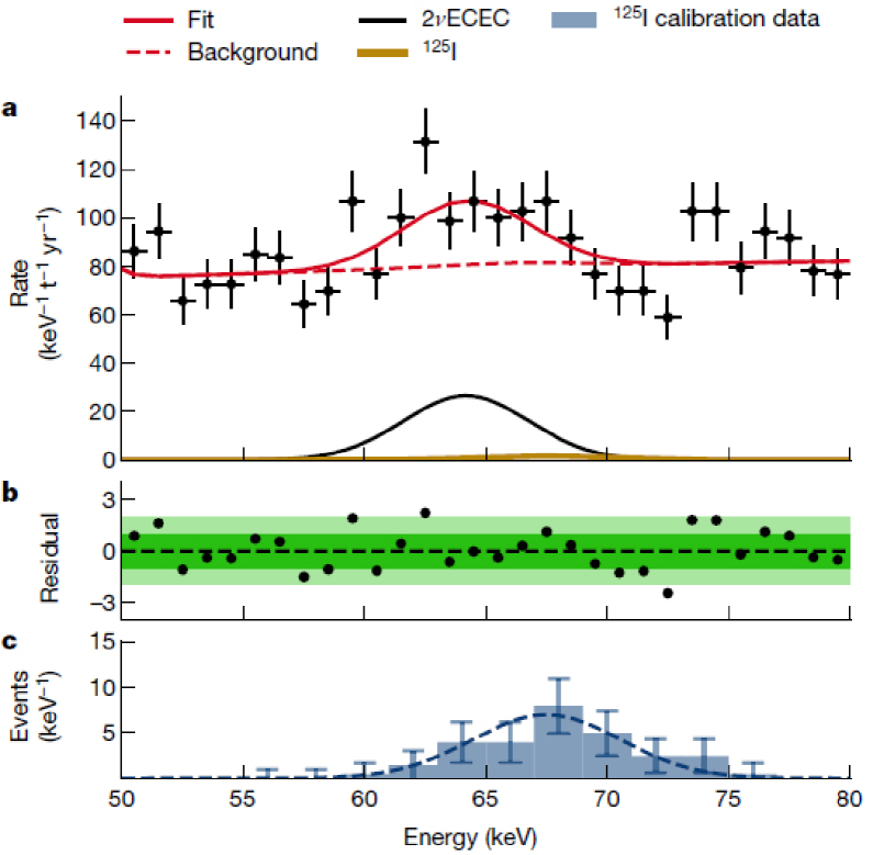
Figure 10: The result of the XENON1t data analysis in the region of interest for $2\nu$2EC in ¹²⁴Xe: (a) $2\nu$2EC decay peak with area 126 events, obtained by the fit of the experimental data, (b) residuals for the experimental data best fit, (c) a histogram of the ¹²⁵I peak produced by neutron activation after the detector calibrations with an external ²⁴¹AmBe neutron source. The peak area in panel (a) corresponds to the half-life of ¹²⁴Xe $1.8\times 10^{22}$ years. For detail see the original work of XENON Collaboration (2019). Reprinted with permission from XENON Collaboration (2019).

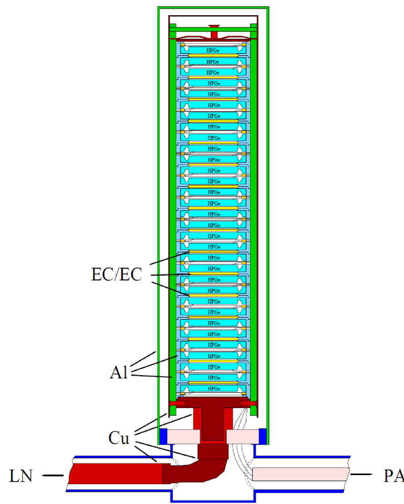
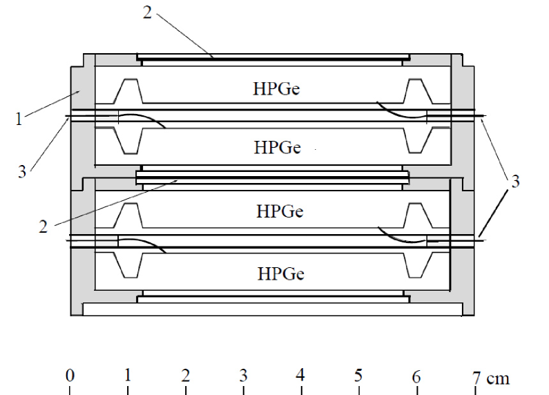
Figure 11: (Color online) Left: Schematic view of the TGV-2 detector. HPGe - planar-type Ge detectors, EC/EC - enriched ¹⁰⁶Cd foils, Al - construction details made from Al-Si alloy, Cu - construction details made from copper, LN - liquid nitrogen, PA - preamplifiers. Right: Section view of the stack of HPGe detectors. 1 - cylindrical holders for the detectors, 2 - ¹⁰⁶Cd foils, 3 - electric contacts (bronze wires in teflon insulators). Reprinted with permission from Rukhadze et al. (2006).

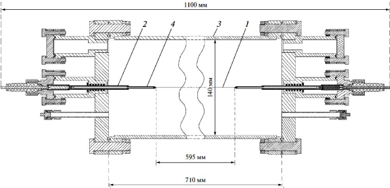
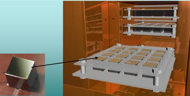
Figure 12: (Color online) Left: Low counting proportional chamber filled with enriched ⁷⁸Kr used in the experiment Gavrilyuk et al. (2013). 1 - Anode wire, 2 - Insulator, 3 - Cathode, 4 - Copper tubes. Reprinted with permission from Gavrilyuk et al. (2010). Right: The concept of the COBRA CdZnTe detectors array. Figure courtesy of K. Zuber.

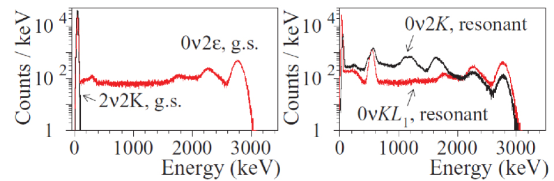
Figure 13: (Color online) Monte Carlo simulated energy spectra of $2\nu KK$, $0\nu$2EC decays of ¹⁰⁶Cd to the ground state of ¹⁰⁶Pd, and neutrinoless resonant transitions of ¹⁰⁶Cd to excited levels in ¹⁰⁶Pd. Reprinted with permission from Belli et al. (2012b).

However, the $\gamma$ spectrometry approach can clearly distinguish the $2\nu$ and $0\nu$ modes of the 2EC decay, too. The $2\nu$2EC decay to the ground state of the daughter nucleus will give a cascade of X-rays and Auger electrons with the individual energies scaling up to the maximal energy of the $K$ X-rays. A combination of X-ray peaks is expected in the decay (as it is shown in Fig. 14 (top) for ¹⁹⁰Pt); X-rays from other atomic shells ($L,M,...$) can be emitted in the $2\nu$2EC, too. However, detection of such small energies by, e.g., HPGe $\gamma$ spectrometry is problematic given that even in the case of one of the heaviest 2EC nuclides ¹⁹⁰Pt the energy of $L$ X rays varies within 9 – 13 keV.

In the process of $0\nu$2EC decay, in addition to X-rays, it is expected that one or more inner-bremsstrahlung photons are emitted carrying off the total decay energy, which in the $2\nu$ process is taken by the neutrinos Rosen and Primakoff (1965). The energy of the $\gamma$ quanta is expected to be equal to $E_{\gamma}=Q-\epsilon^{*}_{\alpha\beta}$, where $\epsilon^{*}_{\alpha\beta}$ is the excitation energy of the atomic shell with two vacancies $\alpha$ and $\beta$ of the daughter nucleus. Therefore, the expected energies of the quanta for the $0\nu$2EC decay to the g.s. of the daughter nucleus are much higher than those in the $2\nu$2EC decay (see Fig. 14 (bottom)).

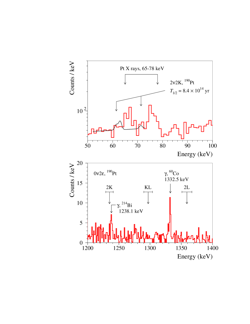
Figure 14: (Color online) (Upper panel) Low-energy part of the spectrum accumulated by a HPGe detector with a platinum sample over 1815 h. The distribution expected for the $2\nu KK$ decay of ¹⁹⁰Pt with a half-life of $8.4\times 10^{14}$ yr excluded at 90% C.L. is shown by a solid line. (Lower panel) Part of the energy spectrum accumulated with the platinum sample in the energy region where peaks from the $0\nu$2EC processes in ¹⁹⁰Pt ($KK,KL$ and $LL$) to the ground state of ¹⁹⁰Os are expected. The error bars take into account the uncertainty of the $Q$-value of 2EC in ¹⁹⁰Pt available at the time when the experiment was realized ($\pm 6$ keV) and different energies of the $L$ X-rays of osmium. Reprinted with permission from Belli et al. (2011d).

There are several reasons for the lower sensitivity of the $2\beta^{+}$ experiments (in comparison to the $2\beta^{-}$ ones). First of all, the development of experimental techniques and the scale of the experiments are rather modest. E.g., the amount of enriched isotopes utilized does not exceed the level of tens of grams, while tens and even hundreds of kilograms of isotopically enriched materials are already used in $2\beta^{-}$ experiments. Then one should take into account the in general much lower abundance of $2\beta^{+}$ active isotopes ($\iota$) in the natural isotopic compositions of elements which is usually lower than 1%. There are only 6 nuclei, namely ⁴⁰Ca ($\iota=96.941\%$), ⁵⁴Fe (5.845%), ⁵⁸Ni (68.0769%), ⁶⁴Zn (49.17%), ⁹²Mo (14.649%) and ⁹⁶Ru (5.54%) from the full list of thirty four double-beta-plus candidates with $\iota$ values greater than 5% Tretyak and Zdesenko (2002); Meija et al. (2016). For comparison, from the full list of thirty five potentially $2\beta^{-}$ decaying nuclides, only 5 candidates have $\iota$ below 5%. It is interesting to note that, starting from ⁷⁴Se, the list of $2\beta^{+}$/EC$\beta^{+}/$2EC nuclei practically coincides with the list of the so-called bypassed (or p-) nuclei Frank-Kamenetsky and G V Domogatsky in: Physics of Cosmos: Small Encyclopedia (1986) which cannot be created in usual r- and s- processes of nucleosynthesis by successive neutron captures, and whose abundances, as a result, are suppressed in comparison to those of r- and s- nuclei.

Finally, the released energy in the $2\beta^{+}$ and EC$\beta^{+}$ decays is lower than that in the $2\beta^{-}$ decays which results in a lower probability for such processes due to the small phase space factors. For $0\nu 2\beta^{-}$ decay processes, because of the relation between half-life $T_{1/2}^{0\nu}$, phase space factor $G_{0\nu}$, NME ($M^{0\nu}$) and $m_{\beta\beta}$: $1/T_{1/2}^{0\nu}=G_{0\nu}|M^{0\nu}|^{2}|m_{\beta\beta}|^{2}$, the lower value of $G_{0\nu}$ for $2\beta^{+}$/EC$\beta^{+}$ processes results in a weaker limit on the effective neutrino mass (or other parameters), even if the same experimental $T_{1/2}$ limit is reached as for the $2\beta^{-}$ decay. To undergo $2\beta^{+}$ decay, the energy release should exceed four electron masses, and only 6 nuclei from the full list of 34 have enough energy for this: ⁷⁸Kr ($Q=2848$ keV), ⁹⁶Ru (2715 keV), ¹⁰⁶Cd (2775 keV), ¹²⁴Xe (2864 keV), ¹³⁰Ba (2619 keV), and ¹³⁶Ce (2379 keV). All these nuclides together with 16 additional nuclides: ⁵⁰Cr, ⁵⁸Ni, ⁶⁴Zn, ⁷⁴Se, ⁸⁴Sr, ⁹²Mo, ¹⁰²Pd, ¹¹²Sn, ¹²⁰Te, ¹⁴⁴Sm, ¹⁵⁶Dy, ¹⁶²Er, ¹⁶⁸Yb, ¹⁷⁴Hf, ¹⁸⁴Os, and ¹⁹⁰Pt, undergo EC$\beta^{+}$ decays for which the released energy should exceed $2m_{e}+\epsilon^{*}_{\alpha}$, where $\epsilon^{*}_{\alpha}$ is the binding energy of the captured electron. And all of these 22 nuclides, together with the 12 remaining ones: ³⁶Ar, ⁴⁰Ca, ⁵⁴Fe, ¹⁰⁸Cd, ¹²⁶Xe, ¹³²Ba, ¹³⁸Ce, ¹⁵²Gd, ¹⁵⁸Dy, ¹⁶⁴Er, ¹⁸⁰W, and ¹⁹⁶Hg, undergo 2EC processes. The lower energy release also results in a lower experimental sensitivity, since the background counting rate typically decreases with energy. In the following we overview the current status of experimental searches of the $2\beta^{+}$, EC$\beta^{+}$ and 2EC processes.

³⁶Ar. The first result for $0\nu KL$ capture in ³⁶Ar, $T_{1/2}^{0\nu}\geq 1.9\times 10^{18}$ yr, was obtained Chkvorets (2008) in the course of the R&D investigations in the GERDA experiment in search for $0\nu 2\beta^{-}$ decay of ⁷⁶Ge using naked HP⁷⁶Ge detectors in liquid argon. It was improved by 3 orders of magnitude with the data from Phase I of the GERDA experiment in underground conditions of the Gran Sasso underground laboratory (LNGS, depth of 3600 m w.e.) where 89.2 t of liquid argon were used as the coolant medium and shield, $T_{1/2}^{0\nu}(KL)>3.6\times 10^{21}$ yr at 90% C.L. Agostini et al. (2016).

⁴⁰Ca. Limits for 2EC decay in ⁴⁰Ca were set in 1999 with the help of two 370 g low radioactive CaF₂(Eu) crystal scintillators at the LNGS over $\simeq 104$ d Belli et al. (1999b). The low energy threshold of 4 keV allowed to also set a limit on the $2\nu$ process, when an energy release in the detector of only 6.4 keV is expected. The achieved $T_{1/2}$ limits (at the level of $10^{21}$ yr) were recently improved slightly with CaWO₄ scintillating bolometers (total exposure of 730 kg d) Angloher et al. (2016) used in the CRESST-II dark matter experiment.

⁵⁰Cr. The first limit on EC$\beta^{+}$ decay of ⁵⁰Cr was set with photographic emulsions to record tracks of $\beta$ particles Fremlin and Walters (1952). The measurements underground at a depth of 570 m gave a half-life limit on the level of $10^{14}$ yr. It was improved in 1985 with two HPGe detectors of 110 cm³ volume each, searching in coincidence for two 511 keV $\gamma$ quanta after annihilation of the emitted positron; measurements of a 148 g Cr sample for 163 h resulted in the limit $T_{1/2}^{0\nu+2\nu}>1.8\times 10^{17}$ yr Norman (1985). The best current EC$\beta^{+}$ sensitivity ($T_{1/2}>1.3\times 10^{18}$ yr) was achieved by Bikit et al. (2003) with a HPGe detector which measured, in coincidence with a NaI(Tl), a 209 g CrO₃ sample for 720 h.

⁵⁴Fe. The only known limits on double-electron capture in ⁵⁴Fe were set in the measurements of Bikit et al. (1998) with the help of a HPGe detector placed in the centre of an iron cube with an inner volume of 1 m³ and a wall thickness of 25 cm. The search for $\gamma$-rays emitted in the 2EC decay for $\simeq 6700$ h gave $T_{1/2}$ limits on the level of $(4.1-5.0)\times 10^{20}$ yr depending on the decay channel ($KK$, $KL$ or $LL$).

⁵⁸Ni. The first limit on EC$\beta^{+}$ decay of ⁵⁸Ni of $\simeq 10^{17}$ yr was reported in an experiment with photoemulsion plates Fremlin and Walters (1952). A level of $\lim T_{1/2}\sim 10^{19}$ yr was reached in an experiment with a Ge(Li) detector and a 2.1 kg Ni sample for 187 h Bellotti et al. (1982), and in measurements with a 1.6 kg Ni sample using two NaI(Tl) scintillators in coincidence for 100 h Norman and DeFaccio (1984). The sensitivity was improved by one order of magnitude in underground measurements at the Baksan Neutrino Observatory of 660 m w.e. depth with two NaI(Tl) scintillators and a 1.9 kg Ni sample Vasil’ev et al. (1993). Further improvement of the sensitivity to the neutrinoless 2EC process of $T_{1/2}>2.1\times 10^{21}$ yr was achieved by using a 7.3 kg Ni sample measured for 1400 h with a low background HPGe detector at the Felsenkeller underground laboratory (110 m w.e.) Lehnert et al. (2016b). The best to date sensitivity was reported by Rukhadze et al. (2018) where a large volume $\approx 600$ cm³ HPGe detector and a 21.7 kg Ni sample installed at the Modane underground laboratory (4800 m w.e.) are used to search for $\gamma$ quanta expected in the 2EC and EC$\beta^{+}$ processes in ⁵⁸Ni. A preliminary limit on the $0\nu$2EC g.s. to g.s. transition in ⁵⁸Ni is $T_{1/2}>4.1\times 10^{22}$ yr.

⁶⁴Zn. Searches for ⁶⁴Zn EC$\beta^{+}$ activity started in 1952 when a Zn sample was measured with photoemulsions Fremlin and Walters (1952). However, no useful limits could be extracted from these data, because the emitted positrons have a quite low energy of $\leq 73$ keV. In 1953, the characteristic X-rays resulting from 2EC decay were searched for with proportional counters. The determined limit was on the level of $10^{16}$ yr Berthelot et al. (1953). In 1985, EC$\beta^{+}$ decay of ⁶⁴Zn was searched for with two HPGe detectors with volume 110 cm³ each looking for 511 keV $\gamma$-rays in coincidence from a 228 g Zn sample. A limit $T_{1/2}^{0\nu+2\nu}>2.3\times 10^{18}$ yr was set after 161 h of measurements Norman (1985).

In 1995, an indication on a positive EC$\beta^{+}$ effect was claimed in measurements (at the Earth’s surface) using a 350 g Zn sample with HPGe and NaI(Tl) detectors in coincidence. After nearly 400 h of data taking an excess of counts in the 511 keV annihilation peak was observed that corresponds to a half-life $T_{1/2}^{0\nu+2\nu}=(1.1\pm 0.9)\times 10^{19}$ yr Bikit et al. (1995). This claim was disproved in two experiments:

(1) Search for double-beta-plus processes in ⁶⁴Zn with emission of $\gamma$ quanta by using a HPGe detector (with volume 456 cm³) and a CsI(Tl) scintillator ($\simeq 400$ cm³) in coincidence. The measurements of a 460 g Zn sample for 375 h at the Cheong Pyung underground laboratory (1000 m w.e.) gave a limit $T_{1/2}^{0\nu+2\nu}>1.3\times 10^{20}$ yr Kim et al. (2007);

(2) A scintillation detector with a 117 g ZnWO₄ crystal scintillator was utilized in an experiment at the LNGS for 1902 h. EC$\beta^{+}$ decay was not observed, the limits $T_{1/2}^{0\nu}>2.2\times 10^{20}$ yr and $T_{1/2}^{2\nu}>2.1\times 10^{20}$ yr were set Belli et al. (2008a). The result was further improved with a larger 0.7 kg detector to $T_{1/2}^{0\nu+2\nu}\geq 9\times 10^{20}$ Belli et al. (2011b).

The 2EC processes in ⁶⁴Zn were searched for in the following experiments:

(1) half-life limits on the 2EC decay of ⁶⁴Zn on level of $10^{17}$ yr were set with the help of a Cd_0.9Zn_0.1Te semiconductor detector with mass 2.89 g over 1117 h of data taking at the LNGS Kiel et al. (2003); the sensitivity was moderately improved in the next stage of the experiment with four Cd_0.9Zn_0.1Te crystals (6.5 g each) Bloxham et al. (2007); advancements of the experiment sensitivity are expected with the currently running set-up with 64 Cd_0.9Zn_0.1Te detectors Ebert et al. (2016b).

(2) ZnWO₄ crystal scintillator, mass of 4.5 g, 429 h of data collection in the Solotvina underground laboratory (1000 m w.e.), half-life limits on the level of $10^{18}$ yr Danevich et al. (2005);

(3) ZnWO₄ scintillators with mass up to 0.7 kg at LNGS Belli et al. (2011b); the strongest to date limits on the 2EC decay of ⁶⁴Zn were set: $T^{2\nu}_{1/2}\geq 1.1\times 10^{19}$ yr and $T^{0\nu}_{1/2}\geq 3.2\times 10^{20}$ yr.

⁷⁴Se. The first search for EC$\beta^{+}$ processes in ⁷⁴Se was performed in measurements of a 563 g Se sample for 437 h with a 400 cm³ HPGe detector and resulted in $T_{1/2}$ limits on the level of $10^{18}-10^{19}$ yr Barabash et al. (2007b), depending on the decay mode ($2\nu$ or $0\nu$) and excited level of the daughter nucleus. The next search for a potentially resonant $LL$ capture of ⁷⁴Se to the 1204 keV level of ⁷⁴Ge was realized in the experiment Frekers et al. (2011) by HPGe $\gamma$ spectrometry of a 3 kg Se sample with a limit $T_{1/2}\geq 4.3\times 10^{19}$ yr. However, this value was corrected to $>1.4\times 10^{18}$ yr by Ješkovský et al. (2015) and re-evaluated further to $>3.9\times 10^{16}$ yr by Lehnert et al. (2016c) for the reason that the method of setting the limit was not reliable enough. In the work by Lehnert et al. (2016c) also the limit Ješkovský et al. (2015) for the $0\nu$2EC transition of ⁷⁴Se to the 1204 keV excited level of ⁷⁴Ge, $T_{1/2}\geq 1.5\times 10^{19}$ yr, obtained with the help of HPGe $\gamma$ spectrometry in coincidence with NaI(Tl) scintillation counter of the same selenium sample as in the experiment Frekers et al. (2011), was re-evaluated to $T_{1/2}\geq 6.3\times 10^{17}$ yr for the same reason of a not quite correct interpretation of the experiment sensitivity as a half-life limit. Lehnert et al. (2016c), after measurements of a $\approx 2.5$ kg selenium sample by using HPGe $\gamma$ detector located in the Felsenkeller Underground Laboratory, gave the strongest to date limit $T_{1/2}\geq 7.0\times 10^{18}$ yr for the $0\nu LL$ transition of ⁷⁴Se to the 1204.2 keV excited state of ⁷⁴Ge.

⁷⁸Kr. ⁷⁸Kr is one of the six nuclides whose $Q$-values allow all three channels of double beta-plus-decays: 2EC, EC$\beta^{+}$ and $2\beta^{+}$. The first experiment to search for EC$\beta^{+}$ and $2\beta^{+}$ decay of ⁷⁸Kr was performed in 1994 with a high pressure ionization chamber placed within an array of 6 large volume ($\simeq 3000$ cm³ each) NaI(Tl) scintillators. The ionization chamber contained 35 lt of enriched (to 94.08%) ⁷⁸Kr. The data were collected in the Canfranc Tunnel Laboratory (675 m w.e.) for 4435 h; derived $T_{1/2}$ limits for $2\beta^{+}$ and EC$\beta^{+}$ processes remain among the best reached for double-beta-plus nuclei ($\simeq 10^{21}$ yr) Saenz et al. (1994).

Experiments Gavriljuk et al. (2000); Gavrilyuk et al. (2011) at the Baksan Neutrino Observatory (BNO, 4900 m w.e.) with enriched ⁷⁸Kr lead to limits at the level of $10^{20}-10^{21}$ yr. An indication on the $2\nu KK$ capture with $T_{1/2}=9.2^{+5.7}_{-2.9}\times 10^{21}$ yr was obtained with a large proportional counter (49 lt) filled by gas enriched in ⁷⁸Kr to 99.81% Gavrilyuk et al. (2013) (recently updated to $1.9^{+1.3}_{-0.8}\times 10^{22}$ yr Ratkevich et al. (2017)). Limits for other modes of decay were also set, in particular, a possible resonant $0\nu KK$ capture to the $2^{+}$ 2838 keV level of ⁷⁸Se was limited as $T_{1/2}\geq 5.4\times 10^{21}$ yr.

⁸⁴Sr. The first limit ($\simeq 10^{13}$ yr) on EC$\beta^{+}$ decay of ⁸⁴Sr was derived by Tretyak and Zdesenko (1995) by analysis of the photoemulsion experiment Fremlin and Walters (1952) with corrections on the decay energy and the natural abundance of the isotope. Recently, 2EC and EC$\beta^{+}$ processes in ⁸⁴Sr has been investigated at a level of $T_{1/2}\sim 10^{15}-10^{16}$ yr with a small (6.6 g) sample of SrI₂(Eu) crystal scintillator measured over 706 h at LNGS by a 468 cm³ HPGe detector Belli et al. (2012a). Furthermore, R&D with a 54 g SrF₂ scintillating bolometer Diaz (2013) allowed to set limits on few decay modes to $T_{1/2}\sim 10^{15}-10^{16}$ yr.

⁹²Mo. A limit on EC$\beta^{+}$ decay of ⁹²Mo can be extracted from a photoemulsion experiment Fremlin and Walters (1952) as $\simeq$10¹⁵ yr. In 1955, double positron tracks emitted from a Mo foil were searched for with a Wilson cloud chamber Winter (1955b). The determined limit of $4\times 10^{18}$ yr should be discarded, because, as we know now, the energy released in the decay is not sufficient for emission of two positrons. Search for 2EC transition of ⁹²Mo to excited levels of ⁹²Zr was realized in 1982 in measurements on the Earth’s surface using a 1.82 kg Mo sample with a 130 cm³ Ge(Li) detector for 161 h, with limits on the level of 10¹⁸ yr Bellotti et al. (1982). In 1985, a 324 g Mo sample was sandwiched between two HPGe detectors (110 cm³ each) looking for coincidence of 511 keV $\gamma$ quanta; $T_{1/2}$ limits of $\simeq$10¹⁷ yr were set Norman (1985). In 1987, positrons emitted from thin Mo foil in EC$\beta^{+}$ decay of ⁹²Mo were searched for with a time projection chamber; after 3.05 h of data taking, limits were set as $10^{17}-10^{18}$ yr Elliott et al. (1987). The best known limits on the double beta decay of ⁹²Mo on the level of $10^{21}$ yr were set in 1995–1997 in underground measurements on 2.5 kg monocrystal Mo rods with a 400 cm³ HPGe detector in the Modane underground laboratory for 1316 h Aunola et al. (1995); Barabash et al. (1997).

The search for EC$\beta^{+}$ decay of ⁹²Mo was also pursued in the YangYang underground laboratory at a depth of 700 m with a 277 g CaMoO₄ crystal scintillator surrounded by 14 big CsI scintillators which served as a passive and active shielding Lee et al. (2011); the achieved limit of $T_{1/2}\geq 2.3\times 10^{20}$ yr is slightly better than the result of Barabash et al. (1997) ($T_{1/2}\geq 1.9\times 10^{20}$ yr). The sensitivity of the experiment Kang et al. (2013), where a 411 g CaMoO₄ crystal was used in coincidence with a HPGe detector, was on the level of $10^{19}-10^{20}$ yr.

⁹⁶Ru. In fact, ⁹⁶Ru is the only nuclide from the list of 6 potential $2\beta^{+}$ decaying nuclides which has an appreciable natural isotopic abundance of $\iota=5.54\%$. Notwithstanding these favourable features for experimental investigation, the first search was performed only in 1985 were a Ru sample of 50 g was measured with two HPGe detectors (110 cm³) in coincidence for 178 h. Determined limits on $2\beta^{+}$ and EC$\beta^{+}$ decays to the ground state and excited levels of ⁹⁶Mo were in the range of 10¹⁶ yr Norman (1985). These limits were improved to the level of $\simeq 10^{19}$ yr by Belli et al. (2009a); Andreotti et al. (2012). The best results on the level of $10^{20}-10^{21}$ yr were obtained at LNGS in measurements with a highly purified Ru sample (mass of 720 g) and four HPGe detectors $\simeq 225$ cm³ each for 5479 h Belli et al. (2013b).

¹⁰²Pd. First $T_{1/2}$ limits on 2EC processes in ¹⁰²Pd were obtained in the experiment at the Felsenkeller underground laboratory, where a 802 g Pd sample was measured with a HPGe detector; the results were on the level of $10^{18}$ yr Lehnert and Zuber (2011). They were improved in measurements with two sandwiched HPGe detectors at the HADES underground laboratory (500 m w.e.) Lehnert et al. (2013). Further measurements were performed at the LNGS in a set-up with four HPGe detectors ($\simeq 225$ cm³ each) for 2093 h; joint analysis of all three measurements pushed the $T_{1/2}$ limits to the level of $10^{19}$ yr Lehnert et al. (2016a).

¹⁰⁶Cd. The nuclide ¹⁰⁶Cd is among the most investigated $2\beta^{+}$ nuclides with a long history of experimental studies. Limits on $2\beta^{+}$ and EC$\beta^{+}$ decays on the level of 10¹⁵ yr can be extracted from the measurements using a Cd sample with photographic emulsions Fremlin and Walters (1952). Searches for positrons emitted in $2\beta^{+}$ decay were performed in 1955 with a Wilson cloud chamber in the magnetic field and a Cd foil with a mass of 30 g; the experiment resulted in a limit of $\simeq$10¹⁶ yr Winter (1955b). In 1984, in measurements of a 153 g Cd sample for 72 h with two NaI(Tl) in coincidence, limits on the level of $\simeq 10^{17}$ yr were determined for $2\beta^{+}$, EC$\beta^{+}$ and 2EC processes Norman and DeFaccio (1984).

An experiment with a ¹¹⁶CdWO₄ crystal scintillator (15 cm³, enriched in ¹¹⁶Cd to 83%) in the Solotvina underground laboratory was aimed at the investigation of $2\beta^{-}$ decay of ¹¹⁶Cd. However, the data collected over 2982 h were also used to set limits for other nuclides, in particular for ¹⁰⁶Cd on the level of 10¹⁷ to 10¹⁹ yr, depending on the decay mode Georgadze et al. (1995). A “source = detector” approach and a low energy threshold allowed to set a limit on $2\nu KK$ capture ($\simeq$10¹⁷ yr) for the first time.

An external Cd foil (331 g) was measured at the Modane underground laboratory with a 120 cm³ HPGe detector for 1137 h, aiming at the detection of $\gamma$ quanta from annihilation of positrons and from de-excitation of the daughter ¹⁰⁶Pd nucleus if the excited levels are populated Barabash et al. (1996). Half-life limits on the level of 10¹⁸–10¹⁹ yr were set. Also in 1996, a large (1.046 kg) CdWO₄ scintillator with natural Cd composition was measured at the LNGS for 6701 h Danevich et al. (1996b). Limits on the half-life for $2\beta^{+}$ and EC$\beta^{+}$ decays were on the level of $\simeq$10¹⁹ yr for $0\nu$, and $\simeq$10¹⁷ yr for $2\nu$ processes. A small (0.5 g) CdTe bolometer operating at a temperature of 10 mK was tested for 72 h by Ito et al. (1997). The derived limit on $0\nu$EC$\beta^{+}$ decay of ¹⁰⁶Cd was 1.4$\times 10^{16}$ yr, lower than those reached with more traditional techniques at that time, particularly due to the small size of the CdTe bolometer.

Cd samples of natural composition with 1.25% of ¹⁰⁶Cd were used in all the above experiments (in ¹¹⁶CdWO₄ scintillator Georgadze et al. (1995) ¹⁰⁶Cd was even depleted). On contrary, a cadmium sample with mass of 154 g enriched by ¹⁰⁶Cd in 68% was used in the experiment Belli et al. (1999a). Measurements at LNGS with two low background NaI(Tl) scintillators for 4321 h enabled to reach a level of the half-life sensitivity of more than 10²⁰ yr for $2\beta^{+}$, EC$\beta^{+}$ and 2EC processes accompanied by emission of $\gamma$ quanta. In 2003, the long-term (14183 h) experiment in the Solotvina underground laboratory with three enriched ¹¹⁶CdWO₄ scintillators (total mass of 330 g) was finished Danevich et al. (2003). Together with measurements for 433 h with a non-enriched CdWO₄ crystal of 454 g, sensitivity for ¹⁰⁶Cd was improved by approximately one order of magnitude in comparison with Georgadze et al. (1995).

A radiopure cadmium tungstate crystal scintillator with a mass of 216 g produced from cadmium enriched in ¹⁰⁶Cd to 66% (¹⁰⁶CdWO₄) was grown in Belli et al. (2010). Measurements at the LNGS gave limits on $2\beta$ processes on the level of $10^{20}$ yr Belli et al. (2012b). In the second stage, the ¹⁰⁶CdWO₄ scintillator was installed between four HPGe detectors ($\simeq 225$ cm³ each) to improve the sensitivity to decay modes accompanied by $\gamma$ quanta; this resulted in limits of $T_{1/2}\geq 10^{20}-10^{21}$ yr Belli et al. (2016). In the third stage, the ¹⁰⁶CdWO₄ detector was running in coincidence with two big CdWO₄ crystal scintillators in a close geometry to increase the detection efficiency of $\gamma$ quanta emitted from the ¹⁰⁶CdWO₄ crystal. The sensitivity of the experiment is approaching the theoretical predictions for the $2\nu$EC$\beta^{+}$ decay of ¹⁰⁶Cd (that are in the interval $10^{21}-10^{22}$ yr): $T_{1/2}\geq 4\times 10^{21}$ yr Polischuk (2019).

At present, there are two other running experiments probing the double-beta decays of ¹⁰⁶Cd: COBRA and TGV-2. The COBRA experiment started at the LNGS with two small semiconductor detectors: Cd_0.9Zn_0.1Te (mass of $\simeq$3 g), and CdTe ($\simeq$6 g) Kiel et al. (2003). CdZnTe crystals are used in the current stage Ebert et al. (2013, 2016a). Results for ¹⁰⁶Cd $T_{1/2}$ limits are on the level of $10^{18}$ yr. The main aim of the TGV-2 experiment (located at the Modane underground laboratory) is the search for $2\nu KK$ decay of ¹⁰⁶Cd (this channel has the lowest expected half-life). In the experiment, 32 planar HPGe detectors are used with a total sensitive volume $\approx 400$ cm³ (see Fig. 11). The Cd foils were enriched in ¹⁰⁶Cd to $60-75$% in the first stage of the experiment Rukhadze et al. (2011b, a, 2006); now 23.2 g of Cd enriched to 99.57% of ¹⁰⁶Cd are used Rukhadze et al. (2016). After $\simeq 8200$ h of data taking, limits are on the level of $10^{20}$ yr.

¹⁰⁸Cd. First limits (10¹⁶–10¹⁷ yr) on 2EC decay of ¹⁰⁸Cd were determined in 1995, with a ¹¹⁶CdWO₄ scintillator in the Solotvina underground laboratory Georgadze et al. (1995). They were improved later to more than 10¹⁷ yr with higher statistics collected (14183 h) and with data of the larger (454 g) CdWO₄ scintillator with natural Cd composition Danevich et al. (2003, 1996a). The best limits on the 2EC decay ($\simeq 10^{18}$ yr) were obtained at LNGS in the COBRA experiment Kiel et al. (2003) and with a CdWO₄ crystal scintillator of 434 g measured for 2758 h in the low-background DAMA/R&D set-up Belli et al. (2008b).

¹¹²Sn. The first limit on the 0$\nu$EC$\beta^{+}$ decay of ¹¹²Sn on the level of $\simeq 10^{13}$ yr was derived by Tretyak and Zdesenko (1995) from the measurements of Sn samples with photographic emulsions Fremlin and Walters (1952). In 2007 bounds on EC$\beta^{+}$ processes in ¹¹²Sn were improved to $\simeq$10¹⁸ yr in an R&D to develop tin-loaded scintillators for $2\beta$ experiments with ¹¹²Sn and ¹²⁴Sn. A 1 lt sample of tetrabutyl-tin (C₄H₉)₄Sn with the Sn concentration of 34% was measured for 140 h with a 456 cm³ HPGe detector in the Cheong Pyung underground laboratory Kim et al. (2007). In another experiment, a 72 cm³ Ge detector was used for measurements of a 1.24 kg Sn sample on the Earth’s surface for 831 h Dawson et al. (2008b). For 2EC processes with population of the ground and excited states of ¹¹²Cd, limits were on the level of $10^{18}$ yr.

In a series of measurements by Dawson et al. (2008a); Barabash et al. (2008); Kidd et al. (2008); Barabash et al. (2009) performed mostly underground with HPGe detectors and external Sn sources (with natural composition and enriched in ¹¹²Sn) limits on the level of $10^{19}-10^{20}$ yr were obtained. Limits in the range of $(0.1-1.6)\times 10^{21}$ yr were achieved with a 100 g Sn sample enriched in ¹¹²Sn to 94.32% measured in the Modane underground laboratory with a 380 cm³ HPGe detector for 3175 h Barabash et al. (2011).

¹²⁰Te. The first limit on $0\nu$EC$\beta^{+}$ decay of ¹²⁰Te ($\simeq 10^{12}$ yr) was determined by Tretyak and Zdesenko (1995) on the basis of the measurements of Te samples with photoemulsions Fremlin and Walters (1952). It was improved to $\simeq 10^{16}$ yr by the COBRA collaboration with small semiconductor detectors Cd_0.9Zn_0.1Te ($\simeq 3$ g, 1117 h of data collection) and CdTe ($\simeq 6$ g, 1645 h) in the LNGS Kiel et al. (2003). Limits on $KK$ captures to the ground state and the first excited level of ¹²⁰Sn were set on the level of 10¹⁶ yr Kiel et al. (2003). Somewhat improved results can be found in Bloxham et al. (2007); Dawson et al. (2009a). The 2EC limits were further improved to $10^{17}-10^{18}$ yr by measuring 1 kg of natural TeO₂ powder with a 400 cm³ HPGe detector for 475 h at the Modane underground laboratory Barabash et al. (2007a). The best results for the EC$\beta^{+}$ mode were obtained in the CUORICINO/CUORE-0 experiments at LNGS with TeO₂ bolometers: $T_{1/2}>2.7\times 10^{21}$ yr for $0\nu$EC$\beta^{+}$ Alduino et al. (2018b) and $T_{1/2}>7.6\times 10^{19}$ yr for $2\nu$EC$\beta^{+}$ Andreotti et al. (2011).

¹²⁴Xe. ¹²⁴Xe has the highest available energy which could be released in $2\beta^{+}$ processes (2864 keV). In the first experiment with a gridded ionization chamber (volume of 3.66 lt), filled with Xe and installed at the Baksan Neutrino Observatory 850 m w.e. underground, the Xe gas of natural composition and Xe sample enriched in ¹³⁶Xe to 93% were measured over 710 h and 685 h, respectively. Limits on $2\beta^{+}$ and EC$\beta^{+}$ decays of ¹²⁴Xe were set in the range of $10^{14}-10^{18}$ yr, depending on the decay mode Barabash et al. (1989). A limit on $2\nu KK$ decay was set by using a multiwire wall-less proportional counter (fiducial volume of 4.44 lt, working pressure of 4.8 atm), also installed at the Baksan Neutrino Observatory but at a larger depth of 4700 m w.e. After the measurements for $\simeq 1600$ h with Xe samples of different isotopic composition, a limit on $2\nu KK$ decay of ¹²⁴Xe was set as $T_{1/2}\geq 1.1\times 10^{17}$ yr Gavriljuk et al. (1998).

Recent developments and the start of the operation of massive dark matter detectors based on Xe allowed to extract limits on $2\nu KK$ decay of ¹²⁴Xe: $T_{1/2}>2.1\times 10^{22}$ yr from 832 kg of liquid Xe at the Kamioka Observatory, Japan (2700 m w.e.) measured for 19200 h Abe et al. (2018), and $T_{1/2}>6.5\times 10^{20}$ yr from the XENON100 TPC with 62 kg of liquid Xe measured at LNGS for 5390 h Aprile et al. (2017). In both these experiments natural Xe was used, with a ¹²⁴Xe abundance of $\iota=0.095\%$. The result from the Baksan Neutrino Observatory, Russia (4900 m w.e.) obtained with 52 g of Xe enriched in ¹²⁴Xe to 21% after 1800 h of measurement with a copper proportional counter is also known: $T_{1/2}>2.5\times 10^{21}$ yr Gavrilyuk et al. (2015). The 2$\nu$2EC in ¹²⁴Xe with a half-life of $T_{1/2}=(1.8\pm 0.5)\times 10^{22}$ yr was finally observed in 2019 by using the XENON1T dark-matter detector XENON Collaboration (2019).

¹²⁶Xe. The limit on ¹²⁶Xe $2\nu KK$ decay was derived in the XMASS experiment: $T_{1/2}>1.9\times 10^{22}$ yr Abe et al. (2018).

¹³⁰Ba. The first limits were derived on the level of 10¹¹ yr for the $2\beta^{+}$ decay and 10¹² yr for the EC$\beta^{+}$ decay Tretyak and Zdesenko (1995) from the experiment with photographic emulsions Fremlin and Walters (1952). In 1996, by re-analyzing the old geochemical measurements Srinivasan (1976) with respect to the amount of the daughter nuclide ¹³⁰Xe accumulated in a BaSO₄ sample during geological time, the limit of $T_{1/2}>4\times 10^{21}$ yr was set for all modes of ¹³⁰Ba decay Barabash and Saakyan (1996). It should be noted that an indication on the effect with $T_{1/2}=2.1^{+3.0}_{-0.8}\times 10^{21}$ yr was obtained for another sample Barabash and Saakyan (1996). A claim on positive observation of the ¹³⁰Ba decay with the half-life $T_{1/2}=(2.16\pm 0.52)\times 10^{21}$ yr (any decay channel and mode) was reported by Meshik et al. (2001) by analysis of ¹³⁰Xe excess in a BaSO₄ sample. It should be stressed that the $T_{1/2}$ value is consistent with the theoretical estimates for the $2\nu KK$ decay of ¹³⁰Ba. The excess of ¹³⁰Xe was also found in another geochemical experiment Pujol et al. (2009) but the obtained half-life was smaller: $T_{1/2}=(6.0\pm 1.1)\times 10^{20}$ yr. In the recent analysis by Meshik and Pravdivtseva (2017), this disagreement was explained by the contribution from cosmogenics, and the result of Meshik et al. (2001) was considered as more reliable.

As for the direct experiments with ¹³⁰Ba, only one experiment was performed in 2004. A BaF₂ crystal scintillator with a mass of 3615 g was measured in coincidence with two NaI(Tl) detectors for 4253 h at LNGS Cerulli et al. (2004). Derived limits on 2$\beta^{+}$ and EC$\beta^{+}$ decays to the ground state and few excited levels of ¹³⁰Xe are on the level of 10¹⁷ yr, far from what is needed to check the possible positive claim of Meshik et al. (2001); Pujol et al. (2009).

¹³²Ba. The first limit for 2EC in ¹³²Ba $T_{1/2}>3.0\times 10^{20}$ yr was set by Barabash and Saakyan (1996) from the re-analysis of the geochemical data on excess of ¹³²Xe in BaSO₄ samples Srinivasan (1976). An excess of ¹³²Xe was observed in the most “promising” barite sample in the already mentioned geochemical measurements Meshik et al. (2001) (in other four samples the ¹³²Xe excess was too large), leading to the ¹³²Ba half-life of $T_{1/2}=(1.3\pm 0.9)\times 10^{21}$ yr. However, for ¹³²Ba the authors preferred more cautiously to give a limit of $T_{1/2}>2.2\times 10^{21}$ yr.

¹³⁶Ce. First limits on $2\beta^{+}$ decay of ¹³⁶Ce were obtained with the help of two CeF₃ crystal scintillators (mass of 75 g and 345 g) measured for 88 h and 693 h, respectively, in the low background set-up at LNGS. In particular, a sensitivity to the $0\nu 2\beta^{+}$ decay was on the level of $T_{1/2}>10^{18}$ yr Bernabei et al. (1997).

Limits for EC$\beta^{+}$ and 2EC processes in ¹³⁶Ce were derived from the long-term (13949 h) measurements with a 635 g Gd₂SiO₅(Ce) crystal scintillator in the Solotvina underground laboratory; the results for $T_{1/2}$ limits were on the level of $10^{13}-10^{16}$ yr, depending on the decay mode Danevich et al. (2001). The limit on $2\nu KK$ capture was later improved from $\simeq$10¹³ yr to $\simeq$10¹⁶ yr in measurements with a CeF₃ scintillation detector (49 g) for 2142 h at LNGS Belli et al. (2003). A small (6.9 g) CeCl₃ scintillator was measured at LNGS for 1638 h also in the “source = detector” approach resulting in half-life limits on the level of $10^{16}-10^{17}$ yr Belli et al. (2011a).

Measurements of Ce-containing materials as external targets with HPGe detectors at LNGS (CeCl₃ 6.9 g, HPGe 244 cm³, 1280 h) Belli et al. (2009b) and CeO₂ 732 g, HPGe 465 cm³, 1900 h Belli et al. (2014)) lead to limits of $\simeq 10^{17}-10^{18}$ yr for modes accompanied by emission of $\gamma$ quanta. The last sample was additionally purified (Th contents in a 627 g sample was reduced by a factor 60) and remeasured for 2299 h with the same detector. This lead to an improvement of $T_{1/2}$ limits to the level of $>10^{18}$ yr Belli et al. (2017).

¹³⁸Ce. In the experiments described above Belli et al. (2014, 2009b); Danevich et al. (2001); Belli et al. (2003, 2011a), the 2EC decays in ¹³⁸Ce were searched for too; the to-date best limits on the neutrinoless $KK$, $KL$ and $LL$ decays are on the level of $(4.0-5.5)\times 10^{17}$ yr Belli et al. (2017).

¹⁴⁴Sm. The first limit on $2\beta$ decay of ¹⁴⁴Sm ($\simeq 8\times 10^{8}$ yr) was obtained recently by Nozzoli (2018) by analysing the average abundances of parent-daughter nuclei in the Earth’s crust. The first counting experiment to search for double-beta processes in ¹⁴⁴Sm by low-background HPGe $\gamma$ spectrometry was performed at the LNGS by using a highly purified samarium oxide sample, with the limits on different channels and modes of 2EC and EC$\beta^{+}$ decays on the level of $T_{1/2}\geq(0.13-1.3)\times 10^{20}$ yr Belli et al. (2019a).

¹⁵²Gd. The first limit on 2EC in ¹⁵²Gd was obtained similarly to ¹⁴⁴Sm as $T_{1/2}>6\times 10^{8}$ yr Nozzoli (2018).

¹⁵⁶Dy. First searches for double beta processes in ¹⁵⁶Dy were realized at the LNGS by measurements of a 322 g sample of dysprosium oxide Dy₂O₃ of 99.98% purity grade with a HPGe detector (244 cm³) for 2512 h Belli et al. (2011c). The obtained limits were on the level of $\simeq 10^{14}-10^{16}$ yr, depending on the decay mode. In the work of Finch and Tornow (2015) two enriched Dy₂O₃ sources (803 mg, enriched in ¹⁵⁶Dy to 21.58%, and 344 mg, 20.9%) were measured at the Kimballton underground research facility, USA (1450 m w.e.) with two HPGe detectors in coincidence. The $T_{1/2}$ limits were improved to the level of $\simeq 10^{17}-10^{18}$ yr.

¹⁵⁸Dy. The limits on 2EC processes in ¹⁵⁸Dy on the level of $T_{1/2}>(0.35-1.0)\times 10^{15}$ yr ($2\nu$ mode) and $T_{1/2}>(0.026-4.2)\times 10^{16}$ yr ($0\nu$) were obtained at LNGS in the experiment by Belli et al. (2011c) described above.

¹⁶²Er. The first limit for ¹⁶²Er $T_{1/2}>5.5\times 10^{8}$ yr was obtained by Nozzoli (2018) similarly to ¹⁴⁴Sm (valid for all decay modes). Much better results close to $10^{18}$ yr for specific transitions were obtained in measurements of a highly-purified Er₂O₃ sample (326 g) with a HPGe detector (465 cm³) for 1934 h at LNGS Belli et al. (2018).

¹⁶⁴Er. The first limit of $T_{1/2}>1.0\times 10^{9}$ yr was obtained byNozzoli (2018) (valid for all 2EC transitions).

¹⁶⁸Yb. The first limit of $T_{1/2}>5.7\times 10^{8}$ yr was obtained by Nozzoli (2018). A much higher sensitivity for different modes and channels of the decay ($\lim T_{1/2}\sim 10^{14}-10^{18}$ yr) was reached in a low-background experiment with a sample of highly purified ytterbium oxide measured by a low-background HPGe detector Belli et al. (2019b).

¹⁷⁴Hf. The first limit $T_{1/2}>5.8\times 10^{8}$ yr was obtained by Nozzoli (2018). The first counting experiment to search for 2EC and EC$\beta^{+}$ decay of ¹⁷⁴Hf was realized using a high-pure 180 g sample of hafnium and the ultra low-background HPGe-detector system located 225 m underground at the HADES laboratory. After 75 days of data taking, limits were set on the level of $T_{1/2}>10^{16}-10^{18}$ yr Danevich et al. (2020).

¹⁸⁰W. First experimental limits on 2EC decays of ¹⁸⁰W were derived in 1995 from measurements with an enriched ¹¹⁶CdWO₄ crystal scintillator (15 cm³) in the Solotvina underground laboratory for 2982 h Georgadze et al. (1995). They were upgraded (to $\simeq 10^{16}$ yr) with three ¹¹⁶CdWO₄ crystals (total mass of 330 g) and higher statistics (14183 h), as well as with measurements for 433 h of a non-enriched CdWO₄ crystal (454 g) Danevich et al. (2003, 1996a). The limits were further improved in measurements at LNGS with ZnWO₄ scintillators to $\simeq 10^{18}$ yr Belli et al. (2011b, 2009c), and with CaWO₄ scintillating bolometers to $\simeq 10^{19}$ yr Angloher et al. (2016).

¹⁸⁴Os. The first limit on EC$\beta^{+}$ decay of ¹⁸⁴Os ($\simeq 10^{10}$ yr) was derived by Tretyak and Zdesenko (1995) from data of the experiment with photoemulsions Fremlin and Walters (1952). Searches for 2EC and EC$\beta^{+}$ decays of ¹⁸⁴Os (including possible resonant $0\nu$2EC transitions) were performed by Belli et al. (2013a) in measurements at the LNGS with a 173 g ultra-pure Os sample and a 465 cm³ HPGe detector for 2741 h; this gave limits of $T_{1/2}\simeq 10^{16}-10^{17}$ yr.

¹⁹⁰Pt. Once again, the first limit on EC$\beta^{+}$ decay of ¹⁹⁰Pt was set from a reanalysis of the photoemulsion experiment Fremlin and Walters (1952) by Tretyak and Zdesenko (1995) with $T_{1/2}\geq 10^{11}$ yr. Recently 2EC decays of ¹⁹⁰Pt with emission of $\gamma$ quanta were searched for at LNGS with a 468 cm³ HPGe detector and a 42 g platinum sample Belli et al. (2011d) for 1815 h; half-life limits were on the level of $10^{16}$ yr.

¹⁹⁶Hg. First experimental limits ($\simeq 10^{17}$ yr) on 2EC in ¹⁹⁶Hg were obtained with a Ge(Li) detector (35 cm³) which was surrounded by a massive (320 kg) Hg shield (containing 480 g of ¹⁹⁶Hg) in the Solotvina underground laboratory for 1478 h Zdesenko and Kuts (1986). The sensitivity was further improved by one order of magnitude in 1990 with the same Hg shielding but with a larger HPGe detector (165 cm³) over 1109 h of data taking Bukhner et al. (1990).

VI.2 Prospects for possible future experiments

There are currently no large-scale projects to search for $0\nu$2EC. However, further research (corrections of atomic mass values, discovery of new excited levels) may lead to the identification of nuclides with favorable conditions for the resonant process. Also detection of $0\nu$2EC process, along with observation of $0\nu 2\beta^{-}$ decay in different nuclei (see discussion, e.g, in Giuliani et al. (2018)), will be requested in a case of positive evidence of $0\nu 2\beta^{-}$ decay in one nuclide. Furthermore, the light neutrino exchange mechanism, being the most favourable one, is not a only possible. The investigations of EC$\beta^{+}$ and $2\beta^{+}$ decay might be one of the tools to identify the mechanism of the decay, whether it is mediated by light neutrino mass or right-handed currents admixture in weak interaction Hirsch et al. (1994). Here we try to give reader an imagination whether high sensitivity $0\nu$2EC experiments are in principle possible.

One can estimate a sensitivity of possible large scale 2EC experiments assuming the performance of the most advanced $2\beta^{-}$ experiments. For instance both the GERDA and Majorana ⁷⁶Ge $2\beta$ experiments achieve a background level of $\sim 10^{-3}$ counts/(yr keV kg) in the region of interest $\sim 2$ MeV Agostini et al. (2018); Elliott et al. (2017). Assuming the use of 100 kg of a highly radiopure isotopically enriched material, HPGe detectors with mass of 100 kg, an energy resolution (full width at half of maximum) of 3 keV, a detection efficiency of $\sim 5\%$, and a measurement time of 5 yr, one can get an estimation of the experimental sensitivity on the level of $\lim T_{1/2}\sim(4-9)\times 10^{25}$ yr. Moreover, there are plans for a ton-scale experiment with HPGe detectors Abgrall et al. (2017) that could further improve the sensitivity.

The bolometric detectors, thanks to their excellent energy resolution and possibility to realize the calorimetric approach with detectors of different chemical formula, look like a very promising approach in the search for resonant 2EC. Using the level of background estimated by the CUORE collaboration $\sim 0.004$ counts/(yr keV kg) Alessandria et al. (2012), a mass of isotope of 100 kg (embedded in highly radiopure crystal scintillators Danevich and Tretyak (2018)) and a detection efficiency around 10% (e.g., in a peak near $Q_{\beta\beta}$ of ¹⁰⁶Cd), one can get an estimation of the experimental sensitivity on the level of $\lim T_{1/2}\sim 4\times 10^{25}$ yr for a 5 years experiment.

It should be stressed one more advantage of possible large scale $0\nu$2EC experiments in comparison to the $0\nu 2\beta^{-}$ searches. In most of the $0\nu$2EC processes closest to resonant ones (see Tables 12 and XIII), the energy of $\gamma$ quanta expected in the decays is many times larger than the energy of the X-ray quanta emitted in the allowed $2\nu$2EC. For instance, in the case of $0\nu$2EC decay of ¹⁵⁶Dy to the $0^{+}$ 1988.5 keV excited level of ¹⁵⁶Gd $\gamma$ quanta with energy 1899.5 keV are expected, while energy of the X-ray quanta in the $2\nu LL$ process in ¹⁵⁶Dy should be within $7.2-8.4$ keV (the binding energies on the $L_{1}$, $L_{2}$ and $L_{3}$ shells of gadolinium atom). Thus, the background due to the $2\nu$2EC mode in an experiment to search for $0\nu$2EC decay to excited level(s) with energy much higher than the energy of X-ray quanta emitted in the $2\nu$2EC decay will never play a role in practice in contrast to the $0\nu 2\beta^{-}$ experiments where background caused by the $2\nu$ mode becomes dominant due to poor energy resolution (scintillation and some gaseous detectors) Tretyak and Zdesenko (1995) or time resolution (low-temperature bolometers) Chernyak et al. (2012). However, for the cases of the g.s. to g.s. resonant transitions (e.g., in ¹⁵²Gd), a very small energy release ($Q_{2\mathrm{EC}}(^{152}$Gd$)=55.7$ keV) makes separation between the effect searched for and the allowed $2\nu KL$ process practically rather problematic.

VI.3 Neutrinoless 2EC with radioactive nuclides

Since there is no clealry identified “ideal nucleus” to find a resonant 2EC among stable (or long-lived) nuclei, it makes sense to consider experiments with radioactive nuclei. Using a few kg of a radioactive material looks challenging but maybe possible taking into account previous experience with e.g. the ⁵¹Cr source for the GALLEX solar neutrino experiment Cribier et al. (1996) or the already started BEST sterile neutrino experiment Barinov et al. (2019). Possibilities of large amounts of radioactive isotopes production for 2EC experiments are discussed in Sec. VII.C.

The most realistic approach to search for $0\nu$2EC decay of radioactive isotopes is $\gamma$ spectrometry. For this purpose one could use a low background HPGe detector array and samples of radioactive material as a source. The isotope should be producible in an amount of tens of kg, should not cause $\gamma$ background in the region of interest, the half-life of the isotope relative to the ordinary decay channel should be long enough to carry out several years of measurements and to avoid thermal destruction of the sample. In the most favorable case the main decay channel of the isotope is low energy $\beta$ (EC) or $\alpha$ decay without $\gamma$-ray emission. The analysis performed by Tretyak et al. (2005) has shown that, despite the very large energy of the $2\beta^{-}$ decay of some radioactive nuclei (and therefore much faster $0\nu 2\beta^{-}$ decay), realization of a high sensitivity experiment will be limited mainly by heat release in the detector. However, while the problem is important in the calorimetry approach requested by $2\beta^{-}$ experiments, it becomes less troublesome in the search for $0\nu$2EC processes by $\gamma$ spectrometry. Nevertheless, taking into account current rather problematic possibilities for production of long-lived radionuclides in large amounts and experimental challenges in ultra-low background measurements with radioactive samples, this approach is still far from practical realization.

VI.4 Section summary

To conclude, the highest up-to-date sensitivity to the $0\nu$2EC decay at the level of $\lim T_{1/2}\sim 10^{21}-10^{22}$ yr is achieved using gaseous (⁷⁸Kr), scintillation (¹⁰⁶Cd), low-temperature bolometric (⁴⁰Ca) detectors, $\gamma$ spectrometry with HPGe detectors (³⁶Ar, ⁵⁸Ni, ⁹⁶Ru, ¹¹²Sn), and geochemical method (¹³⁰Ba, ¹³²Ba). Observation of the allowed two neutrino mode of 2EC decay is claimed only for three nuclides: ⁷⁸Kr, ¹²⁴Xe and ¹³⁰Ba. However, the $2\nu$2EC processes in ⁷⁸Kr and ¹²⁴Xe were detected in a single experiment for each nuclide. Both the claims should be confirmed in independent investigations. As for the geochemical result for ¹³⁰Ba, it needs to be approved by detection in direct counting experiments. The sensitivity to the $0\nu$2EC experiments is $3-4$ orders of magnitude lower than that for the most sensitive $0\nu 2\beta^{-}$ experiments. The main reasons are in general lower sensitivity of the $0\nu$2EC experiments to the absolute neutrino mass (with a similar half-life sensitivity), in most of the cases very low isotopic concentration and limited capabilities of the isotopes of interest enrichment, a more complicated $0\nu$2EC radiative effect signature (which results in a lower detection efficiency to the $0\nu$2EC process), a typically smaller energy release than those for $0\nu 2\beta^{-}$ decays, while the smaller energy of the effect searched for complicates suppression of the radioactive background.

However, the situation might be changed in a case of resonant enhancement of the $0\nu$2EC. In this case $\gamma$ spectrometry of external isotopically enriched source with the help of HPGe diodes, low-temperature bolometers look the most promising detection techniques for possible large scale experiments to search for resonant $0\nu$2EC. In addition to the stable nuclide candidates, searches for the $0\nu$2EC process might be considered in radioactive nuclides with a reasonably long half-life and relevant decay mode which will not interfere with the $0\nu$2EC effect. The most realistic approach in this case could be $\gamma$ spectrometry with HPGe detectors. However, realization of a high sensitivity experiment with radioactive isotope will be limited by practical difficulties of its production in large amounts.

VII Precise determination of 2EC decay energies

The probability of 0$\nu$2EC is in general substantially lower than that of 0$\nu$2$\beta$ decay. The only process that can increase the probability of 0$\nu$2EC and thus make it attractive for its experimental search is its resonant enhancement. Assuming a resonantly enhanced 0$\nu$2EC-transition is found, its use in experiments on the determination of the neutrino type can provide some advantages compared to the investigation of neutrinoless double $\beta^{-}$-decay. First, there might be a variety of excited nuclear states with different low spin values and different parities in one nuclide to which the double-electron-capture transition can be resonantly enhanced resulting in relatively short partial half-lives. Second, no essential reaction induced background from the two-neutrino mode is expected in the case of ground-state-to-ground-state transitions. For two nuclides, connected by transition between the nuclear ground states only, the neutrinoless mode dominates since the two-neutrino transition is strongly suppressed by phase space: no energy is left for the neutrinos to carry away. Thus, in the past ten years experimenters focused on the search for nuclides in which such resonantly enhanced 0$\nu$2EC can take place.

VII.1 Basics of high-precision Penning-trap mass spectrometry

In order to determine the degree of resonant enhancement of the 0$\nu$2EC-transitions, their $Q$-values must be measured with an uncertainty of approximately 100 eV. The $Q$-value is the mass difference of the initial and final states of the transition

$$Q/c^{2}=M_{i}-M_{f}=M_{f}\cdot(\frac{M_{i}}{M_{f}}-1)=M_{f}\cdot(R-1),$$ (VII.1)

where $M_{i}$ and $M_{f}$ are the atomic masses of the initial and final states, respectively, and $R=M_{i}/M_{f}$ their ratio. An uncertainty $\delta Q$ of the $Q$-value determination is given by

$$\delta Q=Q\cdot\sqrt{\left(\frac{\delta M_{f}}{M_{f}}\right)^{2}+\left(\frac{\delta R}{R-1}\right)^{2}}\cong Q\cdot\frac{\delta R}{R-1};R>1,$$ (VII.2)

where $\delta M_{f}$ and $\delta R$ are the uncertainties of the mass of the final state and the mass ratio, respectively. Thus, a determination of the $Q$-value with an uncertainty of a hundred eV implies the measurement of the mass ratio $R$ with an uncertainty of approximately $10^{-9}$.

The only technique which is capable of providing such a low uncertainty for a large variety of stable and radioactive nuclides is nowadays considered to be high-precision Penning-trap mass-spectrometry (PTMS) Blaum et al. (2013); Myers (2013). This technique is superior in achievable sensitivity, accuracy and resolving power to all other mass-measurement methods due to the very idea which forms the basis of a Penning trap: one confines a single ion with mass $M$ and electrical charge $q$ to a minute volume by the superposition of extremely stable and strong static homogeneous magnetic field $B$ and weak static quadrupole electric potential. In such a field configuration a charged particle performs a quite complex periodic motion, which is considered to be a product of three circular motions with very stable eigenfrequencies, namely, cyclotron, magnetron and axial motions with the frequencies $\nu_{+}$, $\nu_{-}$ and $\nu_{z}$, respectively (see Fig. 15) Brown and Gabrielse (1986)).

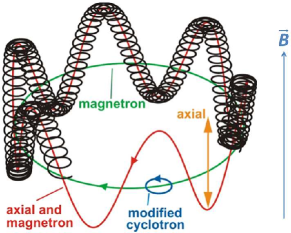
Figure 15: (color online) Motion of an ion in a Penning trap. It can be considered to be a combination of three independent eigenmotions, cyclotron and magnetron motions in the plane orthogonal to the magnetic field lines, and axial motion along the magnetic field line.

A certain combination of these eigenfrequencies yields the so-called free cyclotron frequency

$$\nu_{c}=\frac{1}{2\pi}\cdot\frac{q}{M}\cdot B,$$ (VII.3)

i.e., the frequency of an ion with charge-to-mass ratio $q/M$ in a homogeneous magnetic field $B$. A determination of the mass of a charged particle via a measurement of its free cyclotron frequency, the most precisely measurable quantity in physics, is a remarkable trick which sets the Penning trap beyond any other mass-measurement technique. The measurement of the mass ratio $R$ reduces to the measurement of the ratio $R=\nu_{c}^{f}/\nu_{c}^{i}$ of the cyclotron frequencies $\nu_{c}^{f}$ and $\nu_{c}^{i}$ of the final and initial states of the transition, respectively.

The majority of the Penning-trap facilities are built for mass-measurements on radioactive nuclides and employ for the measurement of the cyclotron frequency the so-called Time-of-Flight Ion-Cyclotron-Resonance technique (ToF-ICR) Gräff et al. (1980); König et al. (1995). A key component of this method is a micro-channel-plate (MCP) detector, which is placed on the axis of the Penning trap (direction $\vec{z}$, see Fig. 17) in a region with very low magnetic field. The MCP detector serves as a counter for single ions. The cyclotron frequency is determined from the measurement of the time of flight (ToF) of the ion passing the strong gradient of the magnetic field between the Penning trap and the MCP detector (Fig. 16).

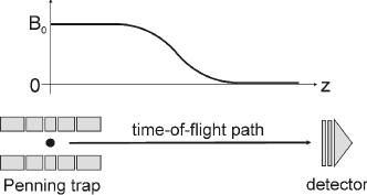
Figure 16: Basic principle of the ToF-ICR technique. The ions are ejected from the trap and sent to the detector through a strong gradient of the magnetic field. The time of flight of the ions depends on their orbital magnetic moment in the trap and is a function of the ion’s cyclotron frequency. For details see text.

An ion in a magnetic-field gradient is subject to a force which acts in direction $\vec{z}$ and is given by

$$\vec{F}=-\frac{E_{r}}{B_{0}}\cdot\frac{\partial B}{\partial z}\cdot\vec{z},$$ (VII.4)

where $E_{r}$ is the ion’s radial kinetic energy and $B_{0}$ is the magnetic field in the trap. The ion’s time of flight between the trap located at zero position and the detector at $z_{det}$ can thus be determined by

$$T(E_{r})=\int_{0}^{z_{det}}dz\cdot\sqrt{\frac{M}{2(E_{0}-qV(z)-\mu(E_{r})B(z))}},$$ (VII.5)

where $E_{0}$ is the total initial energy of the ion, $V(z)$ and $B(z)$ are the electric and magnetic fields along the ion’s path between the trap and MCP detector, and $\mu(E_{r})$ is the ion’s orbital magnetic moment in the Penning trap.

The orbital magnetic moment of the ion in the trap and hence its time of flight can be manipulated by applying a quadrupolar radiofrequency field (rf-field) of certain temporal profile at a frequency near the ion’s cyclotron frequency in the trap. By varying the frequency of the rf-field of duration $T_{rf}$, one obtains the time of flight vs frequency of the rf-field as shown, e.g., in Fig. 17(a) for a one-pulse rf-field König et al. (1995) and in Fig. 17(b) for a two-pulse rf-field Kretzschmar (2007); George et al. (2007a, b).

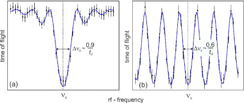
Figure 17: The line shape of the time of flight vs. the (a) one-pulse and (b) two-pulse (Ramsey) rf-field of duration $T_{rf}$, respectively. For details see text.

The two-pulse method (two-pulse Ramsey) is usually the method of choice since it provides the highest precision for the determination of the cyclotron frequency $\nu_{c}$ due to a large number of very pronounced periodic minima in the time-of-flight line shape. The cyclotron frequency of singly charged ions of mass 100 u in a magnetic field of 7 T is approximately 10⁶ Hz. A half-an-hour measurement of the cyclotron frequency with the rf-pulse duration of 2 s and two-pulse Ramsey configuration allows a determination of the cyclotron frequency with a relative uncertainty of about $5\cdot 10^{-9}$ to $10^{-8}$. The final achievable uncertainty of the frequency-ratio determination is usually defined by the instability of the magnetic field in time Droese et al. (2011) and amounts to approximately $10^{-9}$ in the experiments which employ the ToF-ICR detection technique.

Recently, a novel Phase-Image Ion-Cyclotron-Resonance (PI-ICR) technique has been invented Eliseev et al. (2013, 2014) for on-line facilities like SHIPTRAP. In this method the measurement of the ion-cyclotron frequency is based on the projection of the ion position in the trap onto a position-sensitive detector. This allows one to monitor the time evolution of the ion motion and thus to measure the trap-motion frequencies of the ion with subsequent determination of the ion free cyclotron frequency. Compared to the conventional ToF-ICR technique, the PI-ICR offers a gain in precision and resolving power of approximately 5 and 50, respectively. This has made it feasible to carry out measurements of mass ratios of long-lived nuclides with an uncertainty of just a few ten eV at on-line Penning-trap facilities Nesterenko et al. (2014); Eliseev et al. (2015); Karthein et al. (2019).

VII.2 Decay energies of 2EC transitions in virtually stable nuclides

Since 12 out of 19 most promising nuclide pairs from Tables 7 and 8 have been addressed with SHIPTRAP Block et al. (2007) and three pairs have been investigated with the mass-spectrometers JYFLTRAP Kolhinen et al. (2004), TRIGATRAP Ketelaer et al. (2008) and the FSU Penning trap Shi et al. (2005), which are in many aspects similar to SHIPTRAP, the experiments on the determination of the $Q$-values are described here by the example of the SHIPTRAP mass spectrometer.

The SHIPTRAP facility has been built for experiments on transuranium nuclides produced in fusion-evaporation reactions at GSI, Darmstadt. A detailed description of the entire facility can be found in Block et al. (2007). Here, only off-line SHIPTRAP - the part relevant to the measurements of the $Q$-values - is described (Fig. 18).

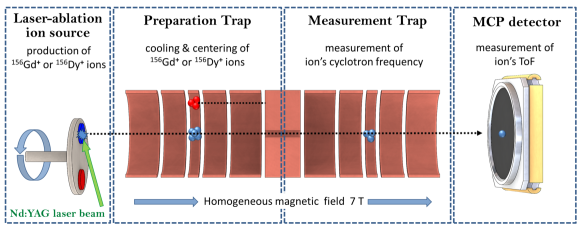
Figure 18: Sketch of the off-line SHIPTRAP facility. The ions produced with a laser ablation are guided by ion transport optics towards the Penning traps. After the mass-selective cooling and centering of the ions in the preparation trap, they are sent into the measurement trap, where their cyclotron frequency is measured with the ToF-ICR technique. For details see text.

The nuclides of interest are virtually stable and can be purchased in sufficient amounts in different chemical forms. For a production of singly charged ions of these nuclides a laser-ablation ion source was used Chaudhuri et al. (2007). For this, a few milligrams of the nuclide of interest were shaped into a 5$\times$5 mm² solid target on a rotatable holder. These targets were then irradiated with short laser pulses. The frequency-doubled Nd:YAG laser (532 nm) has a pulse duration of 3 - 5 ns, a pulse energy of 4 - 12 mJ and a diameter of the laser beam on the target of less than 1 mm. The material is ionized by laser induced desorption, fragmentation and ionization. A series of electrostatic electrodes transport the ions from the ion source towards the Penning-trap mass spectrometer.

The Penning-trap mass spectrometer has two cylindrical Penning traps - the preparation trap (PT) and measurement trap (MT) - placed in a magnetic field of 7 T created by a superconducting magnet. The PT separates the ions of interest from unwanted ions by employing the mass-selective buffer gas cooling technique Savard et al. (1991). From the PT only the ions of interest pass into the MT where their cyclotron frequency is measured with the ToF-ICR technique described above.

The ratio of the cyclotron frequencies of the initial and final nuclides of the transition is obtained by a measurement of the two cyclotron frequencies alternately as schematically depicted in Fig. 19 (left).

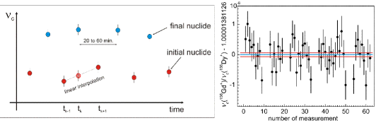
Figure 19: (Colour online) Illustration of the principle of an alternate measurement of the cyclotron frequencies of two nuclides (left) (for details see text), which results in a determination of their ratio (right) (by the example of the frequencies-ratio measurements of ¹⁵⁶Gd and ¹⁵⁶Dy). In the left figure the filled squares and filled circles represent the single measurements of the frequencies of the mother and daughter nuclides, respectively. The hatched circle is the value obtained from the linear interpolation to the time $t_{k}$ of the frequencies measured at times $t_{k-1}$ and $t_{k+1}$. In the right plot the central and upper/lower lines represent the weighted mean frequency ratio and the error of the determination of the weighted mean frequency ratio, respectively.

In this case, the ratio which corresponds, e.g., to measurement time $t_{k}$ (see Fig. 19 (left)) is made up of the frequency of the mother nuclide measured at time $t_{k}$ and the frequency of the daughter nuclide which is obtained by linear interpolation of the frequencies of the daughter nuclide measured at times $t_{k-1}$ and $t_{k+1}$. The measurement time of one ratio-point usually does not exceed 1 hour and is measured with an uncertainty of better than $10^{-8}$. Thus, a measurement campaign of a few-days results in a determination of the frequency ratio with the required uncertainty of about $10^{-9}$, as shown in Fig. 19 (right) by the example of double-electron capture in ¹⁵⁶Dy Eliseev et al. (2011b). The corresponding uncertainty of the $Q$-value is about 100 eV. The results obtained in this measurement campaign are summarized in the review of Eliseev et al. (2012) and included in Tables 7 and 8. The choice of nuclide pairs for measurements was made from the analysis of data for all stable nuclides, which from the energy balance can undergo double electron capture. This data set is presented in Tables 5 and 6. There, in addition to energy, are presented other parameters that allow one to judge the proximity of a particular level to the resonant state, leading to an increase in the probability of double capture. These parameters include the energy gap $\Delta$ and the width $\Gamma$ of the states of electrons undergoing capture, on which the resonance gain factor $R$ depends. The most promising cases were selected for the experiments, the results of which are given in Tables 7 and 8.

Table 7: Parameters of the three most promising 2EC transitions between nuclear ground states which $Q$-values have been precisely measured with SHIPTRAP.

2EC transition	152Gd $\rightarrow$ 152Sm Eliseev et al. (2011c)	164Er $\rightarrow$ 164Dy Eliseev et al. (2012)	180W $\rightarrow$ 180Hf Droese et al. (2012)
electron orbitals	$KL_{1}$	$L_{1}L_{1}$	$KK$
$Q_{\mathrm{2EC}}$ (old) / keV	54.6(35)	23.3(39)	144.4(45)
$\Delta$ (old) / keV	0.27(350)	5.05(390)	12.4(45)
$Q_{\mathrm{2EC}}$ (new) / keV	55.70(18)	25.07(12)	143.20(27)
$\Delta$ (new) / keV	0.83(18)	6.82(12)	11.24(27)

Table 8: 2EC transitions to nuclear excited states which are of interest in the search for the 0$\nu$2EC process and for which $Q_{\mathrm{2EC}}$-values have been precisely measured with Penning traps.

0$\nu$2EC transition	$E^{*}$ / keV	$J_{f}^{\pi}$	electron orbitals	$Q_{\mathrm{2EC}}$ / keV	$\Delta$ / keV	Ref.
74Se $\rightarrow$ 74Ge	1204.205(7)	2+	$L_{2}L_{3}$	1209.169(49)	2.50(5)	Kolhinen et al. (2010)
				1209.240(7)	2.57(1)	Mount et al. (2010)
78Kr $\rightarrow$ 78Se	2838.49(7)	2+	$L_{1}M_{4}$	2847.75(27)	7.55(28)	Bustabad et al. (2013)
			$L_{3}M_{2}$		7.66(28)
96Ru $\rightarrow$ 96Mo	2700.21(6)	2+	$L_{2}L_{2}$	2714.51(13)	9.05(14)	Eliseev et al. (2011a)
102Pd $\rightarrow$ 102Ru	1103.047(13)	2+	$KL_{3}$	1203.27(36)	75.26(36)	Goncharov et al. (2011)
106Cd $\rightarrow$ 106Pd	2748.2(4)	(2,3)-	$KL_{3}$	2775.39(10)	0.33(41)	Goncharov et al. (2011)
112Sn $\rightarrow$ 112Cd	1871.00(19)	0+	$KK$	1919.82(16)	4.50(25)	Rahaman et al. (2009)
120Te $\rightarrow$ 120Sn	?	?	?	1714.81(1.25)	?	Scielzo et al. (2009)
124Xe $\rightarrow$ 124Te	2790.41(9)	0+-4+	$KK$	2856.82(13)	1.96(16)	Nesterenko et al. (2012)
130Ba $\rightarrow$ 130Xe	2544.43(8)	0+	$KK$	2623.71(26)	10.15(26)	Nesterenko et al. (2012)
136Ce $\rightarrow$ 136Ba	2315.32(7)	0+	$KK$	2378.53(27)	11.67(28)	Kolhinen et al. (2011)
144Sm $\rightarrow$ 144Nd	1560.920(13)	2+	$KL_{3}$	1782.59(87)	171.89(87)	Goncharov et al. (2011)
156Dy $\rightarrow$ 156Gd	1946.375(6)	1-	$KL_{1}$	2005.95(10)	0.75(10)	Eliseev et al. (2011b)
	1952.385(7)	0-	$KM_{1}$		1.37(10)
	1988.5(2)	0+	$L_{1}L_{1}$		0.54(24)
	2003.749(5)	2+	$M_{1}N_{3}$		0.04(10)
162Er $\rightarrow$ 162Dy	1782.68(9)	2+	$KL_{3}$	1846.95(30)	2.69(30)	Eliseev et al. (2011a)
168Yb $\rightarrow$ 168Er	1403.7357(23)	2-	$M_{2}M_{2}$	1409.27(25)	1.52(25)	Eliseev et al. (2011a)
184Os $\rightarrow$ 184W	1322.152(22)	0+	$KK$	1453.68(58)	8.89(58)	Smorra et al. (2012)
190Pt $\rightarrow$ 190Os	1326.9(5)	1,2	$KN_{1}$	1401.57(47)	0.14(69)	Eibach et al. (2016)
			$KN_{2}$		0.25(69)
			$KN_{3}$		0.34(69)
			$KN_{4}$		0.51(69)

VII.3 Prospects for measurements of decay energies in radioactive nuclides

The use of radioactive nuclides in the search for 2EC transitions was first proposed by Berlovich and Novikov (1970). Of particular interest were nuclides which are situated very far from the valley of beta-stability. They can undergo double-electron capture with a much higher decay energy than the nuclides along the valley of beta-stability. Since the probability of double-electron capture exhibits a very strong dependence on the $Q_{\mathrm{2EC}}$-value, the half-lives of such nuclides with regard to double-electron capture can be short enough to be measured. Similar to the virtually stable nuclides, also here one could search for resonantly enhanced 0$\nu$2EC by measuring the $Q_{\mathrm{2EC}}$-values of promising 2EC transitions.

The main decay mode of such nuclides must not hamper the search for double-electron capture. In other words, it should be either alpha-decay to a nuclear ground state or electron capture with a low $Q$-value. Furthermore, from practical point of view, the half-lives of such nuclides should be at least a few years. The most promising near-resonant nuclides which fulfill these criteria are listed in Table 9; their specific $0\nu$2EC data are given in Table XIV.

Table 9: Radioactive nuclides with half-lives $T_{1/2}>1$ yr, which might be of interest for $0\nu$2EC. $Q_{\alpha}$ and $T_{1/2}^{\alpha}$ are the $Q$ value and half-life of the $\alpha$-decay mode, respectively. The $Q_{\mathrm{2EC}}$, $Q_{\mathrm{EC}}$ and $Q_{\alpha}$ values and $T_{1/2}^{\mathrm{EC}}$ are from Wang et al. (2017), $T_{1/2}$ are from from the database of Brookhaven National Laboratory (http://www.nndc.bnl.gov/ensdf/).

Mother	$T_{1/2}$	$Q_{\mathrm{2EC}}$	$T_{1/2}^{\mathrm{2EC}\ast)}$	$Q_{\mathrm{EC}}$	$T_{1/2}^{\mathrm{EC}}$	$Q_{\alpha}$	$T_{1/2}^{\alpha}$
nuclide	yr	keV	yr	keV	yr	keV	yr
148Gd	$71.1\pm 1.2$	3066.9(9)	$10^{25-33}$	30(10)	103	3271	70
150Gd	$(1.79\pm 0.08)\times 10^{6}$	1287(6)	$10^{23-33}$	-	-	2807	$(3.00\pm 0.15)\times 10^{6}$
154Dy	$(3.0\pm 1.5)\times 10^{6}$	3312(7)	$10^{23-30}$	-	-	2945	3$\times 10^{6}$
194Hg	$444\pm 77$	2576(3)	$10^{25-31}$	28(4)	103	2698	$\sim 10^{20\ast)}$
202Pb	$(5.25\pm 0.28)\times 10^{4}$	1405(4)	$10^{22-32}$	40(4)	102	2589	$\sim 10^{23\ast\ast)}$

^∗) According to Sec. VIII.

^∗∗) Values estimated with the Geiger-Nuttal approach Brown (1992).

Provided a resonantly enhanced transition has been found in these nuclides by means of Penning-trap mass spectrometry, a suitable mechanism will have to be found for a production of macroquantities of these nuclides. Spalation/fragmentation reactions with high-energy particles and a fusion with heavy ions do not allow the production of a quantity which would be sufficient for a large-scaled experiment in search of 0$\nu$2EC (see Table 10).

Table 10: Estimated yields for the production of the radioactive nuclides of interest for the search for neutrinoless 2EC in spalation/fragmentation reactions with high-energy particles and fusion with heavy ions.

Mother	ISOLDE/CERN ∗)	yield / atoms	yield / atoms	max. counts
nuclide	counts / ions/$\mu$C	(spallation, 3 months)	(fusion with 48Ca, 3 months)	$\mid\lambda$Y$\mid_{2EC}$ / y-1
148Gd	6$\times 10^{8}$	$\approx 10^{16}$	too small
150Gd	4$\times 10^{8}$	$\approx 10^{16}$	$\approx 10^{13}$	$\approx 10^{-7}$
154Dy	8$\times 10^{9}$	$\approx 10^{17}$	$\approx 10^{13}$	$\approx 10^{-6}$
194Hg	7$\times 10^{9}$	$\approx 10^{17}$	$\approx 10^{13}$
202Pb	$10^{7}$	$\approx 10^{14}$	too small	$\approx 10^{-9}$

^∗) http://isolde.web.cern.ch

A more promising production mechanism is an irradiation of samples with neutrons in a reactor. Unfortunately, only relatively short-lived nuclides can be produced in this manner (see Table 11). To calculate the production yields, the mass of the irradiated sample was taken equal to 1 mole, and the neutron flux was 10¹⁵ n/cm²/s. Thus, in principle a production of sufficient amount of ¹⁶⁹Yb and ¹⁷⁵Hf is feasible. However, since these nuclides are too short-lived, their handling might be problematic.

Table 11: Parameters of relatively short-lived nuclides with near-resonant transitions for the search for 0$\nu$2EC, which can be produced in a reactor. The $Q_{\mathrm{EC}}$ and $Q_{\mathrm{2EC}}$-values are in keV units Wang et al. (2017); $E^{*}$ in keV units and $J_{i}^{\pi}$ are from the database of Brookhaven National Laboratory (http://www.nndc.bnl.gov/ensdf/).

nuclide	$J^{\pi}_{i}$	$T_{1/2}^{\mathrm{exp}}$	$Q_{\mathrm{EC}}$	$Q_{\mathrm{2EC}}$	$E^{*}$, possible relevant levels	$\mid\lambda$Y$\mid_{\mathrm{EC}}$ / y-1
					in daughter nuclide	(3 months in reactor)
93Mo	5/2+	$(4.0\pm 0.8)\times 10^{3}$ y	405.8 (15)	315.0 (5)	266.8 (3/2+)	$10^{-3}$
113Sn	1/2+	$115.09\pm 0.03$ d	1039.0 (16)	715.2 (16)	680.52 (3/2+), 708.57 (5/2+)	3$\times 10^{-3}$
145Sm	7/2-	$340\pm 3$ d	616.2 (25)	780.6 (9)	748.275 (9/2-)	$10^{-2}$
169Yb	7/2-	$32.018\pm 0.005$ d	897.6 (11)	545.5 (3)	?	10
175Hf	5/2(-)	$70\pm 2$ d	683.9 (20)	213.9 (23)	?	4

VIII Normalized half-lives of near-resonant nuclides

In this section, estimates of the $0\nu 2$EC half-lives of nuclei closest to the resonance condition are presented. Over the past ten years, great progress has been made due to accurate measurements of $Q_{\mathrm{2EC}}$-values, which made it possible to clarify whether the resonance condition for the prospective nuclides is satisfied (see Sec. VII). The $Q_{\mathrm{2EC}}$ values of the identified earlier prospective nuclides have now been measured.

Table 12: The $0\nu$2EC processes closest to the resonant ones. The normalized half-lives $\tilde{T}_{1/2}$ take newly measured $Q_{\mathrm{2EC}}$ values into account. The 1st column reports the natural isotopic abundance ($\iota$) of the parent nuclides. The spin and parity of the daughter nuclides are given in column 3. If the spin or parity are unknown, their suggested or assumed values are given in round or square brackets, respectively. Column 4 reports the excitation energies of daughter nuclides together with the experimental errors. Column 5 lists the degeneracy parameter of the two atoms $\Delta=M^{**}_{A,Z-2}-M_{A,Z}$, including the excitation energy of the electron shell; the errors indicate the experimental uncertainty in the $Q_{\mathrm{2EC}}$ values. The quantum numbers of the electron vacancies $\alpha$ and $\beta$ are given in the next two columns, where $n$ is the principal quantum number, $j$ is the total angular momentum, and $l$ is the orbital angular momentum. Columns 8, 9 and 10 enumerate the energies of the vacancies $\epsilon_{\alpha}^{*}$ and $\epsilon_{\beta}^{*}$ and the energy shift $\Delta\epsilon_{\alpha\beta}^{*}$ due to the Coulomb interaction, relativistic and collective electron shell effects. Column 11 presents the widths of the excited electron shells. The minimum and maximum normalized half-lives (in years) corresponding to the 99% C.L. interval determined by the uncertainty in the degeneracy parameter $\Delta$ are presented in the last two columns. The masses, energies and widths are given in keV.

$\iota$	Transition	$J^{\pi}_{f}$	$M^{*}_{A,Z-2}-M_{A,Z-2}$	$M^{**}_{A,Z-2}-M_{A,Z}$	$(n2jl)_{\alpha}$	$(n2jl)_{\beta}$	$\epsilon_{\alpha}^{*}\;\;$	$\epsilon_{\beta}^{*}\;\;$	$\Delta\epsilon_{\alpha\beta}^{*}$	$\Gamma_{\alpha\beta}\;\;\;\;\;\;$	$\tilde{T}_{1/2}^{\min}$	$\tilde{T}_{1/2}^{\max}$
5.52%	${}^{96}_{44}$Ru$\to^{96}_{42}$Mo∗∗	0+	2742 $\pm$ 1	28.1 $\pm$ 0.13	310	410	0.50	0.06	0.02	$9.5\times 10^{-3}$	$1.0\times 10^{37}$	$1.3\times 10^{37}$
1.25%	${}^{106}_{~{}48}$Cd$\to^{106}_{~{}46}$Pd∗∗	$[0^{+}]$	2737 $\pm$ 1	11.0 $\pm$ 0.10	110	110	24.35	24.35	0.72	$1.3\times 10^{-2}$	$8\times 10^{31}$	$2\times 10^{32}$
				-10.3 $\pm$ 0.10	110	210	24.35	3.60	0.18	$1.0\times 10^{-2}$	$3\times 10^{32}$	$8\times 10^{32}$
0.095%	${}^{124}_{~{}54}$Xe$\to^{124}_{~{}52}$Te∗∗	[$0^{+}$]	2853.2 $\pm$ 0.6	2.5 $\pm$ 0.12	210	310	4.94	1.01	0.06	$1.2\times 10^{-2}$	$5\times 10^{31}$	$1\times 10^{33}$
				1.6 $\pm$ 0.12	210	410	4.94	0.17	0.02	$4.6\times 10^{-3}$	$2\times 10^{29}$	$3\times 10^{35}$
0.185%	${}^{136}_{~{}58}$Ce$\to^{136}_{~{}56}$Ba∗∗	0+	2315.32 $\pm$ 0.07 ∗)	12.6 $\pm$ 0.27	110	110	37.44	37.44	0.93	$2.6\times 10^{-2}$	$2\times 10^{31}$	$2\times 10^{31}$
		[0+]	2349.5 $\pm$ 0.5	46.7 $\pm$ 0.27	110	110	37.44	37.44	0.93	$2.6\times 10^{-2}$	$2\times 10^{32}$	$2\times 10^{32}$
				14.6 $\pm$ 0.27	110	210	37.44	5.99	0.23	$1.5\times 10^{-2}$	$1\times 10^{32}$	$2\times 10^{32}$
				9.7 $\pm$ 0.27	110	310	37.44	1.29	0.08	$2.4\times 10^{-2}$	$2\times 10^{32}$	$3\times 10^{32}$
		$(1^{+},2^{+})$	2392.1 $\pm$ 0.6	20.9 $\pm$ 0.27	210	310	5.99	1.29	0.05	$1.3\times 10^{-2}$	$3\times 10^{33}$	$5\times 10^{33}$
		$(1^{+},2^{+})$	2399.87 $\pm$ 0.05	64.9$\pm$ 0.27	110	210	37.44	5.99	0.19	$1.5\times 10^{-2}$	$1\times 10^{33}$	$1\times 10^{33}$
0.20%	${}^{152}_{~{}64}$Gd$\to^{152}_{~{}62}$Sm∗	0+	0	39.0 $\pm$ 0.18	110	110	46.83	46.83	1.09	$4.0\times 10^{-2}$	$5\times 10^{31}$	$5\times 10^{31}$
				-0.9 $\pm$ 0.18	110	210	46.83	7.74	0.28	$2.3\times 10^{-2}$	$3\times 10^{28}$	$3\times 10^{29}$
				-1.3 $\pm$ 0.18	110	211	46.83	7.31	0.33	$2.3\times 10^{-2}$	$1\times 10^{31}$	$5\times 10^{31}$
				-7.1 $\pm$ 0.18	110	310	46.83	1.72	0.09	$3.2\times 10^{-2}$	$3\times 10^{31}$	$3\times 10^{31}$
				-8.5 $\pm$ 0.18	110	410	46.83	0.35	0.04	$2.4\times 10^{-2}$	$2\times 10^{32}$	$3\times 10^{32}$
0.06%	${}^{156}_{~{}66}$Dy$\to^{156}_{~{}64}$Gd∗∗	1-	1946.375 $\pm$ 0.006	-1.1 $\pm$ 0.10	110	211	50.24	7.93	0.33	$2.6\times 10^{-2}$	$5\times 10^{29}$	$2\times 10^{30}$
				-7.6 $\pm$ 0.10	110	311	50.24	1.69	0.10	$2.8\times 10^{-2}$	$2\times 10^{32}$	$2\times 10^{32}$
		0-	1952.385 $\pm$ 0.007	5.3 $\pm$ 0.10	110	210	50.24	8.38	0.29	$2.6\times 10^{-2}$	$8\times 10^{31}$	$1\times 10^{32}$
				-1.4 $\pm$ 0.10	110	310	50.24	1.88	0.10	$3.5\times 10^{-2}$	$1\times 10^{31}$	$3\times 10^{31}$
		1-	1962.037 $\pm$ 0.012	14.5 $\pm$ 0.10	110	211	50.24	7.93	0.33	$2.6\times 10^{-2}$	$2\times 10^{32}$	$2\times 10^{32}$
				8.1 $\pm$ 0.10	110	311	50.24	1.69	0.10	$2.8\times 10^{-2}$	$2\times 10^{32}$	$2\times 10^{32}$
		1+	1965.950 $\pm$ 0.004	18.8 $\pm$ 0.10	110	210	50.24	8.38	0.23	$2.6\times 10^{-2}$	$1\times 10^{31}$	$1\times 10^{31}$
				12.2 $\pm$ 0.10	110	310	50.24	1.88	0.08	$3.5\times 10^{-2}$	$2\times 10^{31}$	$2\times 10^{31}$
				10.6 $\pm$ 0.10	110	410	50.24	0.38	0.03	$2.7\times 10^{-2}$	$8\times 10^{31}$	$8\times 10^{31}$
		[$0^{+}$]	1970.2 $\pm$ 0.8	65.8$\pm$ 0.10	110	110	50.24	50.24	1.14	$4.5\times 10^{-2}$	$8\times 10^{31}$	$8\times 10^{31}$
				23.1$\pm$ 0.10	110	210	50.24	8.38	0.29	$2.6\times 10^{-2}$	$5\times 10^{31}$	$8\times 10^{31}$
				16.4$\pm$ 0.10	110	310	50.24	1.88	0.10	$3.5\times 10^{-2}$	$8\times 10^{31}$	$1\times 10^{32}$
		0+	1988.5 $\pm$ 0.2 ∗)	84.1 $\pm$ 0.10	110	110	50.24	50.24	1.14	$4.5\times 10^{-2}$	$1\times 10^{32}$	$1\times 10^{32}$
				41.4 $\pm$ 0.10	110	210	50.24	8.38	0.29	$2.6\times 10^{-2}$	$2\times 10^{32}$	$2\times 10^{32}$
				-0.6 $\pm$ 0.10	210	210	8.38	8.38	0.19	$7.6\times 10^{-3}$	$8\times 10^{25}$	$8\times 10^{30}$
				-1.1 $\pm$ 0.10	210	211	8.38	7.93	0.14	$7.7\times 10^{-3}$	$8\times 10^{31}$	$8\times 10^{32}$
		0+	2026.664 $\pm$ 0.006	79.5 $\pm$ 0.10	110	210	50.24	8.38	0.23	$2.6\times 10^{-2}$	$2\times 10^{32}$	$2\times 10^{32}$
0.14%	${}^{168}_{~{}70}$Yb$\to^{168}_{~{}68}$Er∗∗	1-	1358.898 $\pm$ 0.005	16.7 $\pm$ 0.25	110	211	57.49	9.26	0.36	$3.3\times 10^{-2}$	$8\times 10^{31}$	$1\times 10^{32}$
				9.2 $\pm$ 0.25	110	311	57.49	2.01	0.11	$3.5\times 10^{-2}$	$8\times 10^{31}$	$1\times 10^{32}$
				7.5 $\pm$ 0.25	110	411	57.49	0.37	0.04	$3.4\times 10^{-2}$	$2\times 10^{32}$	$3\times 10^{32}$
		0+	1422.10 $\pm$ 0.03	129.0 $\pm$ 0.25	110	110	57.49	57.49	1.25	$5.7\times 10^{-2}$	$1\times 10^{32}$	$2\times 10^{32}$
0.13%	${}^{180}_{~{}74}$W$\to^{180}_{~{}72}$Hf∗	0+	0	-11.2 $\pm$ 0.27	110	110	65.35	65.35	1.36	$7.2\times 10^{-2}$	$5\times 10^{29}$	$5\times 10^{29}$
				-66.2 $\pm$ 0.27	110	210	65.35	11.27	0.36	$4.2\times 10^{-2}$	$1\times 10^{32}$	$1\times 10^{32}$
0.02%	${}^{184}_{~{}76}$Os$\to^{184}_{~{}74}$W∗∗	$(0)^{+}$	1322.152 $\pm$ 0.022 ∗)	8.8 $\pm$ 0.58	110	110	69.53	69.53	1.42	$8.0\times 10^{-2}$	$2\times 10^{29}$	$3\times 10^{29}$
				-49.6 $\pm$ 0.58	110	210	69.53	12.10	0.37	$4.6\times 10^{-2}$	$3\times 10^{31}$	$5\times 10^{31}$
0.014%	${}^{190}_{~{}78}$Pt$\to^{190}_{~{}76}$Os∗∗	$(0,1,2)^{+}$	1382.4 $\pm$ 0.2 ∗)	7.0 $\pm$ 0.47	210	210	12.97	12.97	0.24	$1.4\times 10^{-2}$	$2\times 10^{31}$	$33\times 10^{31}$
				-3.0 $\pm$ 0.47	210	310	12.97	3.05	0.11	$2.2\times 10^{-2}$	$2\times 10^{30}$	$1\times 10^{31}$
				-3.3 $\pm$ 0.47	210	311	12.97	2.79	0.09	$1.6\times 10^{-2}$	$2\times 10^{32}$	$1\times 10^{33}$
				-5.5 $\pm$ 0.47	210	410	12.97	0.65	0.05	$1.5\times 10^{-2}$	$8\times 10^{31}$	$2\times 10^{32}$

^∗) Decay channels with the known NMEs listed in Table 4.

VIII.1 Decays of virtually stable nuclides

New estimates of the half-lives, taking the recent $Q$-value measurements into account, are presented in Tables 12 and 13. In view of the considerable variance of the NME values for various nuclides (Table 4) and to not mix distinct physical effects, the normalized half-lives $\tilde{T}_{1/2}$ with NME = 3 are provided. In the following we focus mainly on the light Marjorana neutrino exchange mechanism of Fig. 3 (a).

Astrophysical restrictions on the sum of the diagonal neutrino masses obtained by the Planck Collaboration from the study of cosmic microwave background anisotropies yield $\sum m_{\nu}<120$ meV Aghanim et al. (2018). The best restrictions on the effective electron neutrino Majorana mass in double-beta decay experiments are obtained by the KamLAND-Zen Collaboration Gando et al. (2016): $|m_{\beta\beta}|<(61-165)$ meV for commonly used NMEs and the unquenched axial-vector coupling $g_{A}=1.27$. Exotic scalar interactions modify the mass of neutrinos in nuclear matter Kovalenko et al. (2014), so the effective electron neutrino Majorana mass in $0\nu 2\beta^{-}$ decay and $0\nu$2EC can differ from that derived from astrophysical data and tritium beta decay.

The decay half-life is determined by the decay width: $T_{1/2}^{0\nu\mathrm{2EC}}={\ln 2}/{\Gamma_{i}}$, where $\Gamma_{i}$ is given by Eq. (III.8), with $M_{i}=M_{A,Z}$ and $M_{f}=M_{A,Z-2}^{**}$; $\Gamma_{f}\equiv\Gamma_{\alpha\beta}$ is the decay width of the daughter atom with vacancies of electrons in the states $\alpha$ and $\beta$. The amplitude $V_{\alpha\beta}$ entering $\Gamma_{i}$ is defined by Eq. (II.14); for the light Majorana neutrino exchange mechanism, $V_{\alpha\beta}$ simplifies to Eq. (III.23).

Assuming the light Majorana neutrino exchange mechanism is dominant, $T_{1/2}^{0\nu\mathrm{2EC}}$ scales with powers of the overlap factor $K_{Z}$, the neutrino mass $m_{\beta\beta}$, the axial-vector coupling $g_{A}$, and the nuclear matrix element $M_{\mathrm{2EC}}$. The decay half-life can be written as follows:

$$T_{1/2}^{0\nu\mathrm{2EC}}=K_{Z}^{-2}\left(\frac{1.27}{g_{A}}\right)^{4}\left(\frac{100~{}\mathrm{meV}}{|m_{\beta\beta}|}\right)^{2}\left(\frac{3}{|M_{\mathrm{2EC}}|}\right)^{2}\tilde{T}_{1/2}.$$ (VIII.1)

The normalized half-life $\tilde{T}_{1/2}$ does not depend on $K_{Z}$, $m_{\beta\beta}$, $g_{A}$, and $M^{2EC}$. Various schemes for calculating $K_{Z}$ are discussed by Krivoruchenko and Tyrin (2020). The nucleon and non-nucleon spin-isospin correlations and the renormalization effects of the axial-vector coupling $g_{A}$ are discussed in by Ejiri et al. (2019).

Table 13: The normalized half-lives of $0\nu 2$EC processes not included in Table 12, but for which precise $Q_{\mathrm{2EC}}$ values are known, and/or experimental constraints on the $0\nu 2$EC decay half-lives exist. Transitions with $\tilde{T}_{1/2}^{\min}>10^{35}$ y are not shown. An asterisk with a parenthesis ^∗) indicates channels with the known NMEs listed in Table 4. The other notations are the same as in Table 12.

$\iota$	Transition	$J^{\pi}_{f}$	$M^{*}_{A,Z-2}-M_{A,Z-2}$	$M^{**}_{A,Z-2}-M_{A,Z}$	$(n2jl)_{\alpha}$	$(n2jl)_{\beta}$	$\epsilon_{\alpha}^{*}\;\;$	$\epsilon_{\beta}^{*}\;\;$	$\Delta\epsilon_{\alpha\beta}^{*}$	$\Gamma_{\alpha\beta}~{}~{}~{}~{}$	$\tilde{T}_{1/2}^{\min}$	$\tilde{T}_{1/2}^{\max}$
5.52%	${}^{96}_{44}$Ru$\to^{96}_{42}$Mo∗∗	[0+]	2712.68 $\pm$ 0.10 ∗)	1.6 $\pm$ 0.13	210	310	2.87	0.50	0.05	$1.0\times 10^{-2}$	$5\times 10^{32}$	$2\times 10^{33}$
		0+	2742 $\pm$ 1	68.1 $\pm$ 0.13	110	110	20.00	20.00	0.64	$9.0\times 10^{-3}$	$1\times 10^{34}$	$1\times 10^{34}$
1.25%	${}^{106}_{~{}48}$Cd$\to^{106}_{~{}46}$Pd∗∗	[0+]	2717.59 $\pm$ 0.21 ∗)	-8.4 $\pm$ 0.10	110	110	24.35	24.35	0.72	$1.3\times 10^{-2}$	$5\times 10^{31}$	$8\times 10^{31}$
		2,3-	2748.2 $\pm$ 0.4	0.5 $\pm$ 0.10	110	231	24.35	3.17	0.18	$8.3\times 10^{-3}$	$2\times 10^{31}$	$2\times 10^{36}$
0.97%	${}^{112}_{~{}50}$Sn$\to^{112}_{~{}48}$Cd∗∗	0+	1871.00 $\pm$ 0.19	5.4 $\pm$ 0.16	110	110	26.71	26.71	0.76	$1.5\times 10^{-2}$	$1\times 10^{31}$	$2\times 10^{31}$
0.11%	${}^{130}_{~{}56}$Ba$\to^{130}_{~{}54}$Xe∗	(1+)	2533.4 $\pm$ 0.3	-50.2 $\pm$ 0.29	110	210	34.56	5.45	0.18	$1.4\times 10^{-2}$	$8\times 10^{32}$	$8\times 10^{32}$
		(1+)	2544.43 $\pm$ 0.08	-39.1 $\pm$ 0.29	110	210	34.56	5.45	0.18	$1.4\times 10^{-2}$	$5\times 10^{32}$	$5\times 10^{32}$
		(1+)	2628.360$\pm$ 0.001	44.8 $\pm$ 0.29	110	210	34.56	5.45	0.18	$1.4\times 10^{-2}$	$8\times 10^{32}$	$8\times 10^{32}$
		(1+)	2637.50 $\pm$ 0.05	53.9 $\pm$ 0.29	110	210	34.56	5.45	0.18	$1.4\times 10^{-2}$	$1\times 10^{33}$	$1\times 10^{33}$
0.06%	${}^{156}_{~{}66}$Dy$\to^{156}_{~{}64}$Gd∗∗	[0+]	1804 $\pm$ 7	-100.4 $\pm$ 0.10	110	110	50.24	50.24	1.14	$4.5\times 10^{-2}$	$1\times 10^{32}$	$3\times 10^{32}$
		0+	1851.239 $\pm$ 0.007 ∗)	-53.1 $\pm$ 0.10	110	110	50.24	50.24	1.14	$4.5\times 10^{-2}$	$5\times 10^{31}$	$5\times 10^{31}$
0.14%	${}^{162}_{~{}68}$Er$\to^{162}_{~{}66}$Dy∗∗	0+	1666.27 $\pm$ 0.20	-72.0 $\pm$ 0.30	110	110	53.79	53.79	1.19	$5.1\times 10^{-2}$	$5\times 10^{31}$	$8\times 10^{31}$
		1+	1745.716 $\pm$ 0.007	-38.2 $\pm$ 0.30	110	210	53.79	9.05	0.25	$3.0\times 10^{-2}$	$3\times 10^{31}$	$3\times 10^{31}$
1.601%	${}^{164}_{~{}68}$Er$\to^{164}_{~{}66}$Dy∗	0+	0	38.0 $\pm$ 0.12	110	210	53.79	9.05	0.31	$3.0\times 10^{-2}$	$1\times 10^{32}$	$1\times 10^{32}$
0.014%	${}^{190}_{~{}78}$Pt$\to^{190}_{~{}76}$Os∗∗	1,2	1326.9 $\pm$ 0.5 ∗)	-0.1 $\pm$ 0.47	110	410	73.87	0.65	0.07	$5.2\times 10^{-2}$	$3\times 10^{25}$	$2\times 10^{29}$
				-0.2 $\pm$ 0.47	110	411	73.87	0.55	0.04	$5.1\times 10^{-2}$	$5\times 10^{26}$	$3\times 10^{30}$

The value $\Delta\epsilon^{*}_{\alpha\beta}$ shown in Tables 12 - 13 is a correction to the two-hole excitation energy (IV.37). In the lowest approximation, $\Delta\epsilon^{*}_{\alpha\beta}$ is the Coulomb interaction energy of the holes. For the estimates reported here, the values of $\Delta\epsilon^{*}_{\alpha\beta}$ are determined empirically from the Auger electron spectroscopy, as described in Sec. IV.B. If no experimental data are available, $\Delta\epsilon^{*}_{\alpha\beta}$ are determined from calculations using the Grasp2K package. The calculations are performed for noble gas atoms with the simplest electron shell structure. For the remaining atoms with identical quantum numbers of the holes, the interaction energy is obtained via interpolation with a power function $\epsilon^{*}_{\alpha\beta}\sim aZ^{b}$. Tables 12 and 13 report the minimum and maximum normalized values of the half-lives. The confidence interval of the 99% probability is determined by the uncertainty in the degeneracy parameter of the parent and daughter atoms, $M^{**}_{A,Z-2}-M_{A,Z}\pm 2.6\sigma$, where $\sigma^{2}=(\Delta Q)^{2}+(\Delta E^{*})^{2}$ and $\Delta Q$ and $\Delta E^{*}$ are the errors in the $Q_{\mathrm{2EC}}$ value and the excitation energy $E^{*}=M^{*}_{A,Z-2}-M_{A,Z-2}$ of the daughter nuclide, respectively. If this interval includes zero, then at the 99% C.L., the resonance is not excluded, so that $\tilde{T}_{1/2}^{\min}$ gives the unitary limit.

In addition to the perspective nuclear pairs discussed by Krivoruchenko et al. (2011), the $Q_{\mathrm{2EC}}$ values of other nuclide pairs were also measured. Experimental limits on the half-lives of the $0\nu 2$EC decays of some other nuclei were previously known or established in recent years. These additional cases are analyzed on the same grounds; the normalized half-life estimates are presented in Table 13. Decays with a minimum normalized half-life of more than $10^{34}$ years are not listed. Tables 12 and 13 thus report all interesting cases of the atoms for which $Q_{\mathrm{2EC}}$ values were measured and/or the experimental limits on the $0\nu 2$EC half-lives are available.

In the near-resonance region, one finds a group of excited levels of ${}^{130}_{\;\,54}$Xe^∗ with unknown quantum numbers. We provide estimates for four excitation levels of ${}^{130}_{\;\,54}$Xe^∗ with energies $2533.40$, $2544.43$, $2628.36$, and $2637.50$ keV of the assumed spin-parity $1^{+}$. According to our estimates, these decays all appear to be non-resonant. The upper and lower limits of the normalized half-lives coincide with the accuracy under consideration because of small errors in the excitation energy of the daughter nucleus and the precise $Q_{\mathrm{2EC}}$ value of the pair. The same remark applies to the decays ${}^{136}\mathrm{Ce}\to{{}^{136}\mathrm{Ba}^{**}}(2399.9)$, ${}^{156}\mathrm{Dy}\to{{}^{156}\mathrm{Gd}^{**}}(1851.24)$, ${}^{162}\mathrm{Er}\to{{}^{162}\mathrm{Dy}^{**}}(1745.72)$, ${}^{180}\mathrm{W}\to{{}^{180}\mathrm{Hf}^{*}}$, the decay ${}^{156}\mathrm{Dy}\to{{}^{156}\mathrm{Gd}^{**}}(1988.5)$ accompanied by the $KK$ or $KL_{1}$ capture, and to some other decays.

The decay of ¹⁵²Gd is not resonant at 99% C.L., but its probability remains sufficiently high, with a normalized half-life of $3\times 10^{28}-3\times 10^{29}$ years. The case of ¹⁵⁶Dy, which decays into an excited state of gadolinium with energy $1988.5$ keV, is noteworthy. The error in the $Q_{\mathrm{2EC}}$ value of this pair is 100 eV; the resonance capture of electrons from the $L_{1}L_{1}$ state with a normalized half-life of $8\times 10^{25}$ years cannot be excluded at 99% C.L. The NME for decay into the excited level $J^{\pi}=0^{+}$ and the energy of $1851.239$ keV according to Kotila et al. (2014) is equal to 0.35 (Table 4). Taking the same NME value for the level $1988.5$ keV, one finds the half-life of $1.1\times 10^{28}$ years, which is even less than the half-life of ¹⁵²Gd. For other cases considered in Tables 12 and 13, the minimum values of the normalized half-life are above $10^{29}$ years.

VIII.2 Decays of long-lived radionuclides

The radioactive elements are challenging to address experimentally; if one chooses the longest-living ones, then the experimental difficulties in working with such substances may be minimized. We performed an analysis of weakly radioactive elements with lifetimes of longer than a year using the Brookhaven National Laboratory database . From the point of view of resonant capture, two isotopes of gadolinium and isotopes of mercury and lead are of interest. The half-life estimates for these elements are presented in Table XIV. The $Q_{\mathrm{2EC}}$ values of the pairs are not well-known; thus, column five reports two errors in the masses of the parent and daughter nuclei. Column four shows the error in the excitation energy of the daughter nuclide. The first column gives the half-life of the radioactive parent nuclei with respect to the dominant decay. At the present level of knowledge of the parameters of the long-lived radionuclides, any of the channels listed in Table XIV.

Table 14: The near-resonant $0\nu$2EC for long-lived radionuclides. The first column reports the half-life of the parent nuclide. An asterisk with a parenthesis ^∗) indicates channels with the known NMEs listed in Table 4. The fifth column gives the degeneracy parameter, taking into account the excitation energy of the electron shell of the daughter in the ground state. The errors indicate uncertainties in measuring masses of the parent and daughter nuclides, respectively. The other notations are the same as in Table 12.

$T_{1/2}$	Transition	$J^{\pi}_{f}$	$M^{*}_{A,Z-2}-M_{A,Z-2}$	$M^{**}_{A,Z-2}-M_{A,Z}$	$(n2jl)_{\alpha}$	$(n2jl)_{\beta}$	$\epsilon_{\alpha}^{*}\;\;$	$\epsilon_{\beta}^{*}\;\;$	$\Delta\epsilon_{\alpha\beta}^{*}$	$\Gamma_{\alpha\beta}~{}~{}~{}~{}$	$\tilde{T}_{1/2}^{\min}$	$\tilde{T}_{1/2}^{\max}$
$71.1\pm 1.2$ y	${}^{148}_{~{}64}$Gd$\to^{148}_{~{}62}$Sm∗	[0+]	3004 $\pm$ 3 ∗)	-7.5 $\pm$ 2.8 $\pm$ 2.4	110	210	46.83	7.74	0.28	$2.3\times 10^{-2}$	$2\times 10^{25}$	$8\times 10^{31}$
		[1+]		-7.6 $\pm$ 2.8 $\pm$ 2.4	110	210	46.83	7.74	0.22	$2.3\times 10^{-2}$	$8\times 10^{24}$	$8\times 10^{31}$
$71.1\pm 1.2$ y	${}^{148}_{~{}64}$Gd$\to^{148}_{~{}62}$Sm∗∗	[0+]	3022 $\pm$ 3	10.5 $\pm$ 2.8 $\pm$ 2.4	110	210	46.83	7.74	0.28	$2.3\times 10^{-2}$	$2\times 10^{25}$	$1\times 10^{32}$
$(1.79\pm 0.08)\times 10^{6}$ y	${}^{150}_{~{}64}$Gd$\to^{150}_{~{}62}$Sm∗∗	0+	1255.40 $\pm$ 0.22 ∗)	15.4 $\pm$ 6.3 $\pm$ 2.4	110	310	46.83	1.72	0.09	$3.2\times 10^{-2}$	$2\times 10^{26}$	$8\times 10^{32}$
$(3.0\pm 1.5)\times 10^{6}$ y	${}^{154}_{~{}66}$Dy$\to^{154}_{~{}64}$Gd∗∗	1,2+	3264.42 $\pm$ 0.21 ∗)	8.2 $\pm$ 7.6 $\pm$ 2.5	110	210	50.24	8.38	0.23	$2.6\times 10^{-2}$	$5\times 10^{24}$	$3\times 10^{31}$
$444\pm 77$ y	${}^{194}_{~{}80}$Hg$\to^{194}_{~{}78}$Pt∗∗	(0+,1+,2+)	2450 $\pm$ 5 ∗)	-27.6 $\pm$ 12.5 $\pm$ 0.9	110	210	78.39	13.88	0.31	$5.8\times 10^{-2}$	$2\times 10^{24}$	$1\times 10^{31}$
		(0+,1+,2+)	2472 $\pm$ 5 ∗)	-5.6 $\pm$ 12.5 $\pm$ 0.9	110	210	78.39	13.88	0.31	$5.8\times 10^{-2}$	$2\times 10^{24}$	$5\times 10^{30}$
		[1+]	2500 $\pm$ 10 ∗)	22.4 $\pm$ 12.5 $\pm$ 0.9	110	210	78.39	13.88	0.31	$5.8\times 10^{-2}$	$2\times 10^{24}$	$1\times 10^{31}$
$(5.25\pm 0.28)\times 10^{4}$ y	${}^{202}_{~{}82}$Pb$\to^{202}_{~{}80}$Hg∗∗	0+	1411.37 $\pm$ 0.12 ∗)	17.6 $\pm$ 8.2 $\pm$ 0.6	210	310	14.84	3.56	0.12	$2.6\times 10^{-2}$	$2\times 10^{25}$	$2\times 10^{32}$

IX Conclusions

Neutrino physics is a field of science characterized by a wealth of ideas, a multitude of unsolved problems and mysteries that intrigue the imagination. Despite the more than half a century that has passed since the discovery of this particle, it remains the least understood among the fermions of the Standard Model. Great hopes are placed on the study of neutrinoless double-beta ($0\nu 2\beta^{-}$) decay able to shed light on the type of neutrinos (Dirac or Majorana) and on the total lepton number conservation. However, numerous experimental attempts to observe $0\nu 2\beta^{-}$ decay have been unsuccessful so far.

In the steady stream of efforts devoted to the study of $2\beta^{-}$ decay, the reverse process of two-electron capture (2EC) was in the shadows until recently. In this review, a comprehensive characterization of this process is presented, with a main focus on its neutrinoless mode, which can give the same information about the properties of the neutrino as the $0\nu 2\beta^{-}$ decay. All aspects, both theoretical and experimental, revealing in detail unusual physical phenomena associated with the manifestations of the properties of mysterious neutrinos, are considered.

To determine the possibility of observing the neutrinoless 2EC process in real experimental conditions, the lifetimes of nuclides in which the resonant conditions can occur were calculated. For realistic estimates it is necessary to describe properties of electron shells of atoms and 2EC nuclear matrix elements.

Atomic electron shells are involved in the $0\nu 2$EC process through the overlap of the electron wave functions with the nucleus and the excitation energy of electron shells. The short-distance electron wave functions are well defined in the framework of the multielectron Dirac-Hartree-Fock schemes. Valence electrons are bound by several eV, so the excitation energy of the shells is close to the double ionization potential. Experimental progress in atomic spectroscopy made it possible to study multiple ionization processes. Analysis of theoretical uncertainties and comparison with the Auger spectroscopic data leads to the conclusion that the excitation energies of $0\nu 2$EC can be determined with an accuracy of 60 eV or better for heavy atoms, which is comparable to the accuracy in measuring the atomic masses in Penning traps and the de-excitation width of electron shells. An improvement of theoretical schemes or direct measurements of the excitation energy of electron shells with quantum numbers relevant for the $0\nu 2$EC process is of high interest.

The nuclear theory frameworks used to evaluate the nuclear wave functions involved in the nuclear matrix elements of the resonant neutrinoless 2EC transitions cover theories based on the quasiparticle random-phase approximation (both spherical and deformed QRPA), boson mapping (the microscopic interacting boson model, IBM-2) or modern energy-density functionals, EDF. The latter two base the matrix-element computations on the closure approximation and only the QRPA-based theories avoid the use of closure. On the other hand, the IBM-2 and EDF flexibly take into account the deformation degree of freedom, as also to a certain extent the deformed QRPA does.

The most straightforward are the matrix elements involved in the ground-state-to-ground-state captures in the deformed nuclei ¹⁵²Gd, ¹⁵⁶Dy, ¹⁶⁴Er and ¹⁸⁰W. For these nuclides the different theory frameworks (QRPA, IBM-2, EDF) give consistent results within a factor of $2-3$ for the values of the nuclear matrix elements. Theoretical treatment of the excited nuclear resonant states, in particular those with high excitation energies, is a challenge. The problem is the identification of the theoretical state that corresponds to the resonant experimental state of a certain spin-parity, $J^{\pi}$, in particular when there are several experimental and theoretical states close to the resonant state. The intrinsic properties of these close-lying states can vary quite strongly from one state to the next so that selecting the proper state is essential for a reliable prediction of the 2EC nuclear matrix element. This effect is magnified in deformed nuclei, with possible coexisting structures at around similar excitation energies.

At the quark-lepton level, the underlying physical LNV mechanisms of the $0\nu 2$EC, $0\nu$EC$\beta^{+}$, $0\nu 2\beta^{+}$, and $0\nu 2\beta^{-}$ processes are essentially the same. In the Standard Model represented by the sector of renormalized dimensions-4 interactions the total number of leptons $L$ is conserved. The corresponding $\Delta L=2$ contributions can appear via non-renormalizable effective operators of higher dimensions. We specified all the operators up to dimension 9 and discussed their possible high-scale origin from renormalizable theories. We presented, with some detail, three popular large-scale scenarios beyond the Standard Model. The conventional mechanism of Majorana neutrino exchange is highlighted by the fact that the corresponding operator has minimal dimension $d=5$.

The effective electron neutrino Majorana mass $m_{\beta\beta}$ determines the amplitudes of $0\nu 2\beta^{-}$ decay and the $0\nu 2$EC process. We reported the lower and upper half-life limits of $0\nu 2$EC for near-resonant nuclides with the known nuclear matrix elements for the effective electron neutrino Majorana mass of $|m_{\beta\beta}|=100$ meV.

The experimental sensitivity to the $0\nu$2EC process is currently lower as compared to that of the $0\nu 2\beta^{-}$ decay. The strongest $0\nu$2EC half-life limits are at the level of $T_{1/2}\sim 10^{21}-10^{22}$ yr, while the $0\nu 2\beta^{-}$ experiments have already achieved the sensitivity level of $\lim T_{1/2}\sim 10^{24}-10^{26}$ yr. The highest up-to-date sensitivity to the $0\nu$2EC process is achieved using quite diverse experimental techniques: gaseous (⁷⁸Kr), scintillation (¹⁰⁶Cd) and cryogenic scintillating bolometric detectors (⁴⁰Ca), HPGe $\gamma$ spectrometry (³⁶Ar, ⁵⁸Ni, ⁹⁶Ru, ¹¹²Sn), and geochemical methods (¹³⁰Ba, ¹³²Ba).

The prospects for finding $0\nu$2EC become more favorable if a resonance effect in double-electron capture occurs - a phenomenon that is peculiar only to $0\nu$2EC. The resonant $0\nu$2EC effect is expected to be clearly identified thanks to the high accuracy of the $\gamma$ quanta energies expected in the decay, while background due to the neutrino accompanied decay (X-ray with energies up to several tens of keV) will never play a role in practice (in contrast to the $0\nu 2\beta^{-}$ experiments where background caused by the $2\nu$ mode becomes dominant due to poor energy or time resolution). The experimental sensitivity can be significantly improved by increasing the amount of isotopes of interest and utilization of enriched materials, by increasing the detection efficiency, reducing the background and providing the highest possible energy resolution. HPGe detectors and low temperature bolometers appear to be the most suitable detection techniques for $0\nu$2EC experiments with a sensitivity of $T_{1/2}\sim 10^{25}-10^{26}$yr. Moreover, the complicated signature of the resonant effect can be a definite advantage, since the energies of the $\gamma$ quanta expected in most decays are tabulated and usually known with a very high accuracy, which will ensure reliable identification of the effect.

The resonance in 2EC is associated with the degeneracy of mother and intermediate daughter atomic states that can in principle only be fulfilled in 2EC provided the process is neutrinoless. These conditions cannot occur in the 2$\beta^{-}$ decays. However, an insufficiently accurate knowledge of the atomic mass differences between the mother and daughter states has blocked the ascertainment of this possibility so far.

The development of Penning-Trap Mass Spectrometry (PTMS) has radically altered this situation. PTMS is superior to all other known methods of mass spectrometry. It has successfully been used for the determination of mass differences of nuclides with unprecedented low uncertainties down to the eV level. Mass differences for nineteen such pairs connected via 2EC and listed in Tables VII and VIII have been measured by PTMS, and new measurements are still planned for other pairs.

The refined analysis shows that at $90\%$ C.L. none of the stable isotopes are exactly resonant when accompanied by electron capture from favorable states $ns_{1/2}$ and $np_{1/2}$. Yet, at $99\%$ C.L. it is impossible to exclude the exactly resonant character of the ${}^{190}_{~{}78}$Pt$\to^{190}_{~{}76}$Os^∗∗ decay to the excited state 1326.9 $\pm$ 0.5 keV of the daughter. For the vanishing degeneracy parameter and $J^{\pi}=1^{+}$, the half-life appears to be $3.3\times 10^{26}$ years. A more accurate knowledge of the $Q_{\mathrm{2EC}}$-value, the excitation energy and $J^{\pi}$ of ${}^{190}_{~{}76}$Os^∗∗ would certainly be desirable. The ${}^{156}_{~{}66}$Dy$\to^{156}_{~{}64}$Gd^∗∗ decay to the excited state of $1988.5\pm 0.2$ keV also demonstrates the proximity to the resonance. The decay half-life $1.1\times 10^{28}$ years is within the 99% confidence interval. For the ground-to-ground state transitions, the ${}^{152}_{~{}64}$Gd $\to^{152}_{~{}62}$Sm^∗ decay with a lower half-life limit of $7\times 10^{27}$ years is the most encouraging case. The long-lived radionuclides listed in Table XIV can be resonant at $90\%$ C.L., however, production of these nuclides in significant amounts is technically complex.

The data suggests that with further refinement of the parameters, the nuclides under discussion could become competitive with nuclides that decay through the $0\nu 2\beta^{-}$ channel, for which the lower half-life limit is already set at $\sim 10^{26}$ years. This level of sensitivity is also achievable for 2EC processes. Moreover, since not all excited states of nuclides are known experimentally, there can also exist other, not yet identified near-resonant nuclides. Special demands are placed on the nuclear spectroscopy for the search of new relevant excited nuclear states and/or exact determination of the spin and parity values for them.

The search for nuclides satisfying the resonance condition in the 2EC process requires new experimental and theoretical efforts. The experimental side should focus on improving the accuracy of mass measurements by ion traps, the search for new excited states of nuclides in the resonance region, the determination of their excitation energies and quantum numbers, and the determination of the excitation energy of the electron shells using atomic spectroscopy methods. The theory should be aimed at refining theoretical schemes for calculating the 2EC half-life. Further progress requires the joint efforts of theorists in atomic, nuclear and particle physics, as well as the development and implementation of advanced technologies that are already on the horizon. The double-electron capture process can prove to be an important player in the world beyond the Standard Model.

Abbreviations, symbols, and units of measure

$A$	mass number	m w.e.	meters of water equivalent
CC	Charged Current	NME	Nuclear Matrix Element
C.L.	confidence level	PI-ICR	Phase Image Ion Cyclotron Resonance
DEIP	Double-electron Ionization Potential	PMNS	Pontecorvo-Maki-Nakagawa-Sakata mixing matrix
$E^{*}$	excitation energy of nucleus	PTMS	Penning Trap Mass Spectrometry
EDF	Energy Density Functional	PT	Preparation Trap
2EC	double-electron capture	$Q$ value	mass difference between neutral parent and daughter atoms
FWHM	Full Width at Half Maximum	QCD	Quantum Chromodynamics
GCM	Generating Coordinate Method	QED	Quantum Electrodynamics
GT	Gamow-Teller beta-decay type	QRPA	Quasiparticle Random Phase Approximation
g.s.	ground state	RGE	Renormalization Group Equation
HPGe	Hyper-Pure Germanium detector	SEIP	Single-electron Ionization Potential
HO	Harmonic Oscillator	SM	Standard Model
IBM	Interacting Boson Model	SSB	Spontaneous Symmetry Breaking
IBM-2	Microscopic IBM	SUSY	Supersymmetric model
IBFM-2	Microscopic Interacting Boson Fermion Model	RPV	$R$-parity violating
IBFFM-2	Proton-neutron IBFFM	ToF-ICR	Time-of-Flight Ion Cyclotron Resonance
IBFFM	Interacting Boson-Fermion-Fermion Model	$T_{1/2}$	radioactive decay half-life
$K,L,M$, etc.	orbitals of atomic electrons	$Z$	atomic number
LNV	Lepton Number Violation	$0\nu$2EC	neutrinoless double-electron capture
LRSM	Left-Right Symmetric Model	$0\nu 2\beta^{-}$	neutrinoless double-beta decay
LQ	Leptoquarks	$\Gamma$	electromagnetic decay width
$M$	neutral atom mass value	$\Delta$	the degeneracy parameter = $Q$ minus total excitation
			energies of nucleus and electron shells
MCP	Micro-Channel Plate	$\epsilon^{*}$	excitation energy of electron shell
MCM	Multiple-Commutator Model	$\nu$	neutrino
MT	Measurement Trap	$\nu_{i}$	ion frequencies in the trap

References

- Abe et al. (2015) Abe, K, Y. Hayato, T. Iida, K. Ishihara, J. Kameda, Y. Koshio, et al. (2015), “Search for oscillation in Super-Kamiokande,” Phys. Rev. D 91, 072006.
- Abe et al. (2018) Abe, K, et al. (2018), “Improved search for two-neutrino double electron capture on 124Xe and 126Xe using particle identification in XMASS-I,” Prog. Theor. Exp. Phys. 053D03.
- Abgrall et al. (2017) Abgrall, N, et al. (2017), “The large enriched germanium experiment for neutrinoless double beta decay (LEGEND),” AIP Conf. Proc. 1894, 020027.
- Aghanim et al. (2018) Aghanim, N, et al. (2018), “Planck 2018 results. VI. Cosmological parameters,” arXiv:1807.06209 .
- Agostini et al. (2016) Agostini, M, et al. (2016), “Limit on the radiative neutrinoless double electron capture of 36Ar from GERDA Phase I,” Eur. Phys. J. C 76, 652.
- Agostini et al. (2018) Agostini, M, et al. (2018), “Improved Limit on Neutrinoless Double- Decay of 76Ge from GERDA Phase II,” Phys. Rev. Lett. 120, 132503.
- Albert et al. (2018) Albert, J B, et al. (2018), “Search for Neutrinoless Double-Beta Decay with the Upgraded EXO-200 Detector,” Phys. Rev. Lett. 120, 072701.
- Alduino et al. (2018a) Alduino, C, et al. (2018a), “First Results from CUORE: A Search for Lepton Number Violation via Decay of 130Te,” Phys. Rev. Lett. 120, 132501.
- Alduino et al. (2018b) Alduino, C, et al. (2018b), “Search for neutrinoless EC decay of 120Te with CUORE-0,” Phys. Rev. C 97, 055502.
- Alessandria et al. (2012) Alessandria, F, et al. (2012), “CUORE crystal validation runs: Results on radioactive contamination and extrapolation to CUORE background,” Astropart. Phys. 35, 839–849.
- Anastasio et al. (1983) Anastasio, M R, L. S. Celenza, W. S. Pong, and C. M. Shakin (1983), “Relativistic nuclear structure physics,” Phys. Rep. 100, 327–392.
- Andreotti et al. (2012) Andreotti, E, M. Hult, G. Marissens, R. González de Orduña, and P. Vermaercke (2012), “Study of the double beta decays of 96Ru and 104Ru,” Appl. Radiat. Isot. 70, 1985–1989.
- Andreotti et al. (2011) Andreotti, E, et al. (2011), “Search for /EC double beta decay of 120Te,” Astropart. Phys. 34, 643–648.
- Angloher et al. (2016) Angloher, G, et al. (2016), “New limits on double electron capture of 40Ca and 180W,” J. Phys. G 43, 095202.
- Aprile et al. (2017) Aprile, E, et al. (2017), “Search for two-neutrino double electron capture of 124Xe with XENON100,” Phys. Rev. C 95, 024605.
- Arbeláez et al. (2016) Arbeláez, C, M. González, M. Hirsch, and S. G. Kovalenko (2016), “QCD Corrections and Long-Range Mechanisms of neutrinoless double beta decay,” Phys. Rev. D 94, 096014.
- Arbeláez et al. (2017) Arbeláez, C, M. González, S. G. Kovalenko, and M. Hirsch (2017), “QCD-improved limits from neutrinoless double beta decay,” Phys. Rev. D 96, 015010.
- Arnold et al. (2015) Arnold, R, et al. (2015), “Results of the search for neutrinoless double- decay in 100Mo with the NEMO-3 experiment,” Phys. Rev. D 92, 072011.
- Aunola et al. (1995) Aunola, M, J. Suhonen, A. S. Barabash, V. I. Umatov, R. Gurrián, F. Hubert, and Ph. Hubert (1995), “Double beta processes in 92Mo,” JETP Lett. 62, 706–709.
- Avignone III et al. (2008) Avignone III, F T, S. R. Elliott, and J. Engel (2008), “Double beta decay, Majorana neutrinos, and neutrino mass,” Rev. Mod. Phys. 80, 481 – 516.
- Ayala et al. (2020) Ayala, C, G. Cvetic, and L. Gonzalez (2020), “Evaluation of neutrinoless double beta decay: QCD running to sub-GeV scales,” Phys. Rev. D 101, 094003.
- Azzolini et al. (2018) Azzolini, O, et al. (2018), “First Result on the Neutrinoless Double- Decay of 82Se with CUPID-0,” Phys. Rev. Lett. 120, 232502.
- Band and Trzhaskovskaya (1986) Band, I M, and M. B. Trzhaskovskaya (1986), “Electron-Wave-Function Expansion Amplitudes Near the Origin Calculated in the Dirac-Fock-Slater and Dirac-Fock Potentials,” At. Data. Nucl. Data Tables 35, 1–13.
- Barabash (2018) Barabash, A S (2018), “Main features of detectors and isotopes to investigate double beta decay with increased sensitivity,” Int. J. Mod. Phys. A 33, 1843001.
- Barabash et al. (1997) Barabash, A S, R. Gurriarán, E. Hubert, Ph. Hubert, and V. L. Umatov (1997), “Improved limits on double beta processes in 92Mo,” Z. Phys. A 357, 351–352.
- Barabash et al. (2007a) Barabash, A S, F. Hubert, Ph. Hubert, and V. Umatov (2007a), “New limits on the EC and ECEC processes in 120Te,” J. Phys. G 34, 1721–1728.
- Barabash et al. (2011) Barabash, A S, Ph. Hubert, Ch. Marquet, A. Nachab, S. I. Konovalov, F. Perrot, F. Piquemal, and V. Umatov (2011), “Improved limits on EC and ECEC processes in 112Sn,” Phys. Rev. C 83, 045503.
- Barabash et al. (2009) Barabash, A S, Ph. Hubert, A. Nachab, S. I. Konovalov, and V. Umatov (2009), “Search for EC and ECEC processes in 112Sn,” Phys. Rev. C 80, 035501.
- Barabash et al. (2008) Barabash, A S, Ph. Hubert, A. Nachab, S. I. Konovalov, I. A. Vanyushin, and V. Umatov (2008), “Search for EC and ECEC processes in 112Sn and decay of 124Sn to the excited states of 124Te,” Nucl. Phys. A 807, 269–281.
- Barabash et al. (2007b) Barabash, A S, Ph. Hubert, A. Nachab, and V. Umatov (2007b), “Search for EC and ECEC processes in 74Se,” Nucl. Phys. A 785, 371–380.
- Barabash et al. (1989) Barabash, A S, V. V. Kuzminov, V. M. Lobashev, V. M. Novikov, B. M. Ovchinnikov, and A. A. Pomanskyl (1989), “Results of the experiment on the search for double beta decay of 136Xe, 134Xe and 124Xe,” Phys. Lett. B 223, 273–276.
- Barabash and Saakyan (1996) Barabash, A S, and R. R. Saakyan (1996), “Experimental limits on 2, , and processes for 130Ba and on capture for 132Ba,” Phys. At. Nucl. 59, 179–184.
- Barabash et al. (1996) Barabash, A S, V. I. Umatov, R. Gurriarán, F. Hubert, Ph. Hubert, M. Aunola, and J. Suhonen (1996), “Theoretical and experimental investigation of the double beta processes in 106Cd,” Nucl. Phys. A 604, 115–128.
- Barinov et al. (2019) Barinov, V, V. Gavrin, V. Gorbachev, D. Gorbunov, and T. Ibragimova (2019), “BEST potential in testing the eV-scale sterile neutrino explanation of reactor antineutrino anomalies,” Phys. Rev. D 99, 111702(R).
- Belli et al. (2011a) Belli, P, R. Bernabei, F. Cappella, R. Cerulli, F. A. Danevich, A. d’Angelo, A. Di Marco, A. Incicchitti, F. Nozzoli, and V. I. Tretyak (2011a), “Search for decay of cerium isotopes with CeCl3 scintillator,” J. Phys. G 38, 015103.
- Belli et al. (2011b) Belli, P, R Bernabei, F. Cappella, R. Cerulli, F. A. Danevich, S. d’Angelo, A. Incicchitti, V. V. Kobychev, D. V. Poda, and V. I. Tretyak (2011b), “Final results of an experiment to search for processes in zinc and tungsten with the help of radiopure ZnWO4 crystal scintillators,” J. Phys. G 38, 115107.
- Belli et al. (2009a) Belli, P, R. Bernabei, F. Cappella, R. Cerulli, F. A. Danevich, S. d’Angelo, A. Incicchitti, M. Laubenstein, O. G. Polischuk, D. Prosperi, and V. I. Tretyak (2009a), “Search for double- decays of 96Ru and 104Ru by ultra-low background HPGe spectrometry,” Eur. Phys. J. A 42, 171.
- Belli et al. (2009b) Belli, P, R. Bernabei, S. d’Angelo, F. Cappella, R. Cerulli, A. Incicchitti, M. Laubenstein, D. Prosperi, and V. I. Tretyak (2009b), “First limits on neutrinoless resonant captures in 136Ce and new limits for other processes in 136Ce and 138Ce isotopes,” Nucl. Phys. A 824, 101–114.
- Belli et al. (1999a) Belli, P, R. Bernabei, A. Incicchitti, C. Arpesella, V. V. Kobychev, O. A. Ponkratenko, V. I Tretyak, and Yu. G. Zdesenko (1999a), “New limits on 2 decay processes in 106Cd,” Astropart. Phys. 10, 115–120.
- Belli et al. (1999b) Belli, P, et al. (1999b), “New limits on spin-dependent coupled WIMPs and on processes in 40Ca and 46Ca by using low radioactive CaF2(Eu) crystal scintillators,” Nucl. Phys. B 563, 97–106.
- Belli et al. (2003) Belli, P, et al. (2003), “Performances of a CeF3 crystal scintillator and its application to the search for rare processes,” Nucl. Instrum. Meth. A 498, 352–361.
- Belli et al. (2008a) Belli, P, et al. (2008a), “Search for 2 processes in 64Zn with the help of ZnWO4 crystal scintillator,” Phys. Lett. B 658, 193–197.
- Belli et al. (2008b) Belli, P, et al. (2008b), “Search for double- decay processes in 108Cd and 114Cd with the help of the low-background CdWO4 crystal scintillator,” Eur. Phys. J. A 36, 167–170.
- Belli et al. (2009c) Belli, P, et al. (2009c), “Search for double beta decay of zinc and tungsten with low background ZnWO4 crystal scintillators,” Nucl. Phys. A 826, 256–273.
- Belli et al. (2010) Belli, P, et al. (2010), “Development of enriched 106CdWO4 crystal scintillators to search for double decay processes in 106Cd,” Nucl. Instrum. Meth. A 615, 301–306.
- Belli et al. (2011c) Belli, P, et al. (2011c), “First search for double decay of dysprosium,” Nucl. Phys. A 859, 126–139.
- Belli et al. (2011d) Belli, P, et al. (2011d), “First search for double- decay of platinum by ultra-low background HPGe spectrometry,” Eur. Phys. J. A 47, 91.
- Belli et al. (2012a) Belli, P, et al. (2012a), “Radioactive contamination of SrI2(Eu) crystal scintillator,” Nucl. Instr. Meth. A 670, 10–17.
- Belli et al. (2012b) Belli, P, et al. (2012b), “Search for double- decay processes in 106Cd with the help of a 106CdWO4 crystal scintillator,” Phys. Rev. C 85, 044610.
- Belli et al. (2013a) Belli, P, et al. (2013a), “First search for double- decay of 184Os and 192Os,” Eur. Phys. J. A 49, 24.
- Belli et al. (2013b) Belli, P, et al. (2013b), “Search for decays of 96Ru and 104Ru by ultralow-background HPGe spectrometry at LNGS: Final results,” Phys. Rev. C 87, 034607.
- Belli et al. (2014) Belli, P, et al. (2014), “Search for double beta decay of 136Ce and 138Ce with HPGe gamma detector,” Nucl. Phys. A 930, 195–208.
- Belli et al. (2016) Belli, P, et al. (2016), “Search for double- decay in 106Cd with an enriched 106CdWO4 crystal scintillator in coincidence with four HPGe detectors,” Phys. Rev. C 93, 045502.
- Belli et al. (2017) Belli, P, et al. (2017), “New limits on , and decay of 136Ce and 138Ce with deeply purified cerium sample,” Eur. Phys. J. A 53, 172.
- Belli et al. (2018) Belli, P, et al. (2018), “First search for and decay of 162Er and new limit on decay of 170Er to the first excited level of 170Yb,” J. Phys. G 45, 095101.
- Belli et al. (2019a) Belli, P, et al. (2019a), “First direct search for 2 and decay of 144sm and decay of 154sm,” Nucl. Phys. A 55, 201.
- Belli et al. (2019b) Belli, P, et al. (2019b), “First search for and processes in 168yb,” Nucl. Phys. A 990, 64–78.
- Bellotti et al. (1982) Bellotti, E, E. Fiorini, C. Liguori, A. Pullia, A. Sarracino, and L. Zanotti (1982), “An experimental investigation on lepton number conservation in double-beta processes,” Lett. Nuovo Cimento 33, 273.
- Berestetsky et al. (1982) Berestetsky, V B, E M Lifshitz, and L P Pitaevsky (1982), Quantum Electrodynamics (Pergamon, Oxford).
- Berger et al. (1984) Berger, J F, M. Girod, and D. Gogny (1984), “Microscopic analysis of collective dynamics in low energy fission,” Nucl. Phys. A 428, 23–36.
- Berlovich and Novikov (1970) Berlovich, E E, and Yu. N. Novikov (1970), “Probability of Double Beta Decay of Nuclei in Regions Far Removed from the Beta-Stable Band,” Soviet Physics Doklady 14, 986–988.
- Bernabei et al. (1997) Bernabei, R, P. Belli, A. Incicchitti, D. Prosperi, C. Bacci, F. De Notaristefani, G. J. Davies, and C. J. Dai (1997), “Feasibility of decay searches with Ce isotopes using CeF3 scintillators,” Nuovo Cim. A 110, 189–195.
- Bernabeu et al. (1983) Bernabeu, J, A. De Rujula, and C. Jarlskog (1983), “Neutrinoless double electron capture as a tool to measure the electron neutrino mass,” Nucl. Phys. B 223, 15–28.
- Bernabeu and Segarra (2018) Bernabeu, J, and A. Segarra (2018), “Stimulated transitions in resonant atom Majorana mixing,” JHEP 02, 017.
- Berthelot et al. (1953) Berthelot, A, R. Chaminade, C. Levi, and L. Papineau (1953), “Recherche d’une double capture K dans le zinc (64),” Comptes Rendus 236, 1769.
- Bialynicki-Birula (1970) Bialynicki-Birula, I (1970), “Renormalization, diagrams, and gauge invariance,” Phys. Rev. D 2, 2877–2886.
- Bikit et al. (1995) Bikit, I, M. Krmar, J. Slivka, I. Aničin, M. Veskovic, and Lj. Čonkič (1995), “Electron-positron conversion decay of 64Zn,” Appl. Radiat. Isot. 46, 455–456.
- Bikit et al. (1998) Bikit, I, M. Krmar, J. Slivka, M. Vesković, Lj. Čonkić, and I. Aničinl (1998), “New results on the double decay of iron,” Phys. Rev. C 58, 2566.
- Bikit et al. (2003) Bikit, I, N. Zikić-Todorović, J. Slivka, M. Vesković, M. Krmar, Lj. Ćonkić, J. Puzović, and I. V. Aničin (2003), “Double decay of 50Cr,” Phys. Rev. C 67, 065801.
- Bilenky (2018) Bilenky, S (2018), Introduction to the Physics of Massive and Mixed Neutrinos, 2nd edition, Lecture Notes in Physics, vol. 947 (Springer-Verlag, Berlin Heidelberg).
- Bilenky and Giunti (2015) Bilenky, S M, and C. Giunti (2015), “Neutrinoless double-beta decay: A probe of physics beyond the standard model,” Int. J. Mod. Phys. A 30, 1530001.
- Bilenky and Petcov (1987) Bilenky, S M, and S. T. Petcov (1987), “Massive neutrinos and neutrino oscillations,” Rev. Mod. Phys. 59, 671 – 754.
- Bjorken and Drel (1965) Bjorken, JD, and S. D. Drel (1965), Relativistic quantum fields (McGraw-Hill).
- Blaum (2006) Blaum, K (2006), “High-accuracy mass spectrometry with stored ions,” Phys. Rep. 425, 1–78.
- Blaum et al. (2013) Blaum, K, J. Dilling, and W. Nörtershäuser (2013), “Precision atomic physics techniques for nuclear physics with radioactive beams,” Phys. Scr. T 152, 014017.
- Block et al. (2007) Block, M, et al. (2007), “Towards direct mass measurements of nobelium at SHIPTRAP,” Eur. Phys. J. D 45, 39–45.
- Bloxham et al. (2007) Bloxham, T, et al. (2007), “First results on double -decay modes of Cd, Te, and Zn isotopes,” Phys. Rev. C 76, 025501.
- Bogoliubov and Shirkov (1980) Bogoliubov, N N, and D. V. Shirkov (1980), Introduction to the Theory of Quantized Field, 3rd ed. (John Wiley & Sons Inc.).
- Bohr and Mottelson (1969) Bohr, A, and B. R. Mottelson (1969), Nuclear Structure, Vol. I (Benjamin, New York).
- Bollen et al. (1987) Bollen, G, et al. (1987), “First absolute mass measurements of short-lived isotopes,” Hyperfine Interact. 38, 793 – 802.
- Bonnet et al. (2013) Bonnet, F, M. Hirsch, T. Ota, and W. Winter (2013), “Systematic decomposition of the neutrinoless double beta decay operator,” J. High Energy Phys. 03, 55.
- Brant and Paar (1988) Brant, S, and V. Paar (1988), “IBFFM Yrast States in Odd-Odd Nuclei Associated with (6) and (3) Limits,” Z. Phys. A 329, 151–159.
- Breit (1929) Breit, G (1929), “The Effect of Retardation on the Interaction of Two Electrons,” Phys. Rev. 34, 553–573.
- Brockmann and Machleidt (1984) Brockmann, R, and R. Machleidt (1984), “Nuclear saturation in a relativistic Brueckner-Hartree-Fock approach,” Phys. Lett. B 149, 283–287.
- Brown (1992) Brown, B A (1992), “Simple relation for alpha decay half-lives,” Phys. Rev. C 46, 811–814.
- Brown and Gabrielse (1986) Brown, L S, and G. Gabrielse (1986), “Geonium theory: Physics of a single electron or ion in a Penning trap,” Rev. Mod. Phys. 58, 233–311.
- Broyles (1988) Broyles, A A (1988), “Relativistic equation for the multielectron atom,” Phys. Rev. 38, 1137–1148.
- Buchmüller et al. (1987) Buchmüller, W, R. Rückl, and D. Wyler (1987), “Leptoquarks in lepton-quark collisions,” Phys. Lett. B 191, 442–448.
- Bukhner et al. (1990) Bukhner, E, et al. (1990), “Rare decays of mercury nuclei,” Sov. J. Nucl. Phys. 52, 193–197.
- Bunge et al. (1993) Bunge, C F, J. A. Barrientos, and A. V. Bunge (1993), “Roothaan-Hartree-Fock Ground-State Atomic Wave Functions: Slater-Type Orbital Expansions and Expectation Values for ,” At. Data. Nucl. Data Tables 53, 113–162.
- Bustabad et al. (2013) Bustabad, S, G. Bollen, M. Brodeur, D. L. Lincoln, S. J. Novario, M. Redshaw, R. Ringle, and S. Schwarz (2013), “Examination of the possible enhancement of neutrinoless double-electron capture in 78Kr,” Phys. Rev. C 88, 035502.
- Campbell and Papp (2001) Campbell, J L, and T. Papp (2001), “Width of the atomic – levels,” At. Data. Nucl. Data Tables 77, 1–56.
- Cerulli et al. (2004) Cerulli, R, P. Belli, R. Bernabei, F. Cappella, F. Nozzoli, F. Montecchi, A. d’Angelo, A. Incicchitti, D. Prosperi, and C. J. Dai (2004), “Performances of a BaF2 detector and its application to the search for decay modes in 130Ba,” Nucl. Instrum. Meth. A 525, 535–543.
- Chaudhuri et al. (2007) Chaudhuri, A, et al. (2007), “Carbon-cluster mass calibration at SHIPTRAP,” Eur. Phys. J. D 45, 47–53.
- Chernyak et al. (2012) Chernyak, D M, F. A. Danevich, A. Giuliani, E. Olivieri, M. Tenconi, and V. I. Tretyak (2012), “Random coincidence of decay events as a background source in bolometric decay experiments,” Eur. Phys. J. C 72, 1989.
- Chkvorets (2008) Chkvorets, O (2008), “Search for double beta decay with HPGe detectors at the Gran Sasso underground laboratory, Ph.D. thesis, University of Heidelberg (2008),” arXiv:0812.1206 [nucl-ex] .
- Cirigliano et al. (2018a) Cirigliano, V, W. Dekens, J. de Vries, M. L. Graesser, and E. Mereghetti (2018a), “A neutrinoless double beta decay master formula from effective field theory,” JHEP 1812, 097.
- Cirigliano et al. (2018b) Cirigliano, V, W. Dekens, J. de Vries, M. L. Graesser, and E. Mereghetti (2018b), “Neutrinoless double beta decay in chiral effective field theory: lepton number violation at dimension seven,” JHEP 1812, 082.
- Cirigliano et al. (2017) Cirigliano, V, W. Dekens, J. De Vries, M. L. Graesser, E. Mereghetti, S. Pastore, and U. Van Kolck (2017), “Neutrinoless double beta decay and chiral ,” Phys. Lett. B 769, 460.
- Cirigliano et al. (2018c) Cirigliano, V, W. Dekens, J. De Vries, M. L. Graesser, E. Mereghetti, S. Pastore, and U. Van Kolck (2018c), “New Leading Contribution to Neutrinoless Double- Decay,” Phys. Rev. Lett. 120, 202001.
- Cirigliano et al. (2019) Cirigliano, V, W. Dekens, J. De Vries, M. L. Graesser, E. Mereghetti, S. Pastore, M. Piarulli, U. Van Kolck, and R. B. Wiringa (2019), “Renormalized approach to neutrinoless double- decay,” Phys. Rev. C 100, 055504.
- Cirigliano et al. (2020) Cirigliano, V, W. Detmold, A. Nicholson, and Ph. Shanahan (2020), “Lattice QCD Inputs for Nuclear Double Beta Decay,” arXiv:2003.08493 [nucl-th] .
- Clementi and Roetti (1974) Clementi, E, and C. Roetti (1974), “Roothaan-Hartree-Fock atomic wavefunctions: Basis functions and their coefficients for ground and certain excited states of neutral and ionized atoms, ,” At. Data. Nucl. Data Tables 14, 177–478.
- Cremonesi and Pavan (2014) Cremonesi, O, and M. Pavan (2014), “Challenges in Double Beta Decay,” Adv. High Energy Phys. 2014, 951432.
- Cribier et al. (1996) Cribier, M, et al. (1996), “Production of a 62 PBq 51Cr low energy neutrino source for GALLEX,” Nucl. Instrum. Meth. A 378, 233–250.
- Danevich et al. (1996a) Danevich, F A, A. Sh. Georgadze, V. V. Kobychev, B. N. Kropivyansky, V. N. Kuts, A. S. Nikolayko, O. A. Ponkratenko, V. I. Tretyak, and Yu. G. Zdesenko (1996a), “Beta decay of 113Cd,” Phys. At. Nucl. 59, 1–5.
- Danevich et al. (2020) Danevich, F A, M. Hult, D. V. Kasperovych, G. P. Kovtun, K. V. Kovtun, G. Lutter, G. Marissens, O. G. Polischuk, S. P. Stetsenko, and V. I. Tretyak (2020), “First search for and decay of 174Hf,” Nucl. Phys. A (submitted) .
- Danevich et al. (2005) Danevich, F A, V. V. Kobychev, S. S. Nagorny, D. V. Poda, V. I. Tretyak, S. S. Yurchenko, and Yu. G. Zdesenko (2005), “ZnWO4 crystals as detectors for 2 decay and dark matter experiments,” Nucl. Instrum. Meth. A 544, 553–564.
- Danevich et al. (2001) Danevich, F A, V. V. Kobychev, O. A. Ponkratenko, V. I. Tretyak, and Yu. G. Zdesenko (2001), “Quest for double beta decay of 160Gd and Ce isotopes,” Nucl. Phys. A 694, 375–391.
- Danevich and Tretyak (2018) Danevich, F A, and V. I. Tretyak (2018), “Radioactive contamination of scintillators,” Int. J. Mod. Phys. A 33, 1843007.
- Danevich et al. (1996b) Danevich, F A, et al. (1996b), “Investigation of and /EC decay of 106Cd,” Z. Phys. A 355, 433–437.
- Danevich et al. (2003) Danevich, F A, et al. (2003), “Search for 2 decay of cadmium and tungsten isotopes: final results of the Solotvina experiment,” Phys. Rev. C 68, 035501.
- Darwin (1920) Darwin, C E (1920), “The dynamical motions of charged particles,” The London, Edinburgh, and Dublin Philosophical Magazine and Journal of Science 39, 537–551.
- Dawson et al. (2008a) Dawson, J, D. Degering, M. Köhler, R. Ramaswamy, C. Reeve, J. R. Wilson, and K. Zuber (2008a), “Search for double- decays of tin isotopes with enhanced sensitivity,” Phys. Rev. C 78, 035503.
- Dawson et al. (2008b) Dawson, J, R. Ramaswamy, C. Reeve, J. R. Wilson, and K. Zuber (2008b), “A search for various double beta decay modes of tin isotopes,” Nucl. Phys. A 799, 167–180.
- Dawson et al. (2009a) Dawson, J V, C. Goessling, B. Janutta, M. Junker, T. Koettig, D. Muenstermann, S. Rajek, C. Reeve, O. Schulz, J. R. Wilson, and K. Zuber (2009a), “Experimental study of double- decay modes using a CdZnTe detector array,” Phys. Rev. C 80, 025502.
- Dawson et al. (2009b) Dawson, J V, et al. (2009b), “Experimental study of double- decay modes using a CdZnTe detector array,” Phys. Rev. C 80, 025502.
- Delion and Suhonen (2017) Delion, D S, and J. Suhonen (2017), “Two-neutrino decays and low-lying Gamow-Teller strength functions in the mass range A = 70-176,” Phys. Rev. C 95, 034330.
- Dell’Oro et al. (2016) Dell’Oro, S, S. Marcocci, M. Viel, and F. Vissani (2016), “Neutrinoless Double Beta Decay: 2015 Review,” Adv. High Energy Phys. 2016, 2162659.
- Desclaux (1973) Desclaux, J P (1973), “Relativistic Dirac-Fock expectation values for atoms with to ,” At. Data. Nucl. Data Tables 12, 311–406.
- Diaz (2013) Diaz, C G (2013), “Characterization of scintillating bolometers for particle detection and installation of a bolometric test facility in the University of Zaragoza,” PhD thesis, Univ. Zaragoza .
- Doi et al. (1985) Doi, M, T. Kotani, and E. Takasugi (1985), “Double Beta Decay and Majorana Neutrino,” Prog. Theor. Phys. Suppl. 83, 1–175.
- Dover et al. (1983) Dover, C B, A. Gal, and J. M. Richard (1983), “Neutron-antineutron oscillations in nuclei,” Phys. Rev. D 27, 1090–1100.
- Dover et al. (1985) Dover, C B, A. Gal, and J. M. Richard (1985), “Limits on the neutron-antineutron oscillation time from the stability of nuclei,” Phys. Rev. C 31, 1423–1429.
- Droese et al. (2011) Droese, C, M. Block, M. Dworschak, S. Eliseev, E. Minaya Ramirez, D. Nesterenko, and L. Schweikhard (2011), “Investigation of the magnetic field fluctuation and implementation of a temperature and pressure stabilization at SHIPTRAP,” Nucl. Instrum. Methods A 632, 157–163.
- Droese et al. (2012) Droese, C, et al. (2012), “Probing the nuclide 180W for neutrinoless double-electron capture exploration,” Nucl. Phys. A 875, 1–7.
- Dyall et al. (1989) Dyall, K G, I. P. Grant, C. T. Johnson, F. A. Parpia, and E. P. Blummer (1989), “GRASP: A general-purpose relativistic atomic structure program,” Comput. Phys. Comm. 55, 425–456.
- Ebert et al. (2013) Ebert, J, et al. (2013), “Current status and future perspectives of the COBRA experiment,” Adv. High Energy Phys. 2013, 703572.
- Ebert et al. (2016a) Ebert, J, et al. (2016a), “Results of a search for neutrinoless double- decay using the COBRA demonstrator,” Phys. Rev. C 94, 024603.
- Ebert et al. (2016b) Ebert, J, et al. (2016b), “The COBRA demonstrator at the LNGS underground laboratory,” Nucl. Instrum. Meth. A 807, 114–120.
- Eibach et al. (2016) Eibach, M, G Bollen, K Gulyuz, C Izzo, M Redshaw, R Ringle, R Sandler, and A A Valverde (2016), “Double resonant enhancement in the neutrinoless double-electron capture of 190Pt,” Phys. Rev. C 94, 015502.
- Ejiri et al. (2019) Ejiri, H, J. Suhonen, and K. Zuber (2019), “Neutrino-nuclear responses for astro-neutrinos, single beta decays and double beta decays,” Phys. Rep. 797, 1–102.
- Eliseev et al. (2013) Eliseev, S, K. Blaum, M. Block, C. Droese, M. Goncharov, E. Minaya Ramirez, D. A. Nesterenko, Yu. N. Novikov, and L. Schweikhard (2013), “Phase-Imaging Ion-Cyclotron-Resonance Measurements for Short-Lived Nuclides,” Phys. Rev. Lett. 110, 082501.
- Eliseev et al. (2007) Eliseev, S, M. Block, A. Chaudhuri, F. Herfurth, H.-J. Kluge, A. Martin, C. Rauth, and G. Vorobjev (2007), “Octupolar excitation of ions stored in a Penning trap mass spectrometer – A study performed at SHIPTRAP,” Int. J. Mass Spectrom. 262, 45–50.
- Eliseev et al. (2011a) Eliseev, S, D. Nesterenko, K. Blaum, M. Block, C. Droese, F. Herfurth, E. Minaya Ramirez, Yu. N. Novikov, L. Schweikhard, and K. Zuber (2011a), “ values for neutrinoless double-electron capture in 96Ru, 162Er, and 168Yb,” Phys. Rev. C 83, 038501.
- Eliseev et al. (2012) Eliseev, S, Yu. N. Novikov, and K. Blaum (2012), “Search for resonant enhancement of neutrinoless double-electron capture by high-precision Penning-trap mass spectrometry,” J. Phys. G 39, 124003.
- Eliseev et al. (2011b) Eliseev, S, et al. (2011b), “Multiple-resonance phenomenon in neutrinoless double-electron capture,” Phys. Rev. C 84, 012501(R).
- Eliseev et al. (2011c) Eliseev, S, et al. (2011c), “Resonant Enhancement of Neutrinoless Double-Electron Capture in 152Gd,” Phys. Rev. Lett. 106, 052504.
- Eliseev et al. (2014) Eliseev, S, et al. (2014), “A phase-imaging technique for cyclotron-frequency measurements,” Appl. Phys. B 114, 107–128.
- Eliseev et al. (2015) Eliseev, S, et al. (2015), “Direct Measurement of the Mass Difference of 163Ho and 163Dy Solves the Q-Value Puzzle for the Neutrino Mass Determination,” Phys. Rev. Lett. 115, 062501.
- Elliott (2012) Elliott, S R (2012), “Recent progress in double beta decay,” Mod. Phys. Lett. A 27, 1230009.
- Elliott and Franz (2015) Elliott, S R, and M. Franz (2015), “: Majorana fermions in nuclear, particle, and solid-state physics,” Rev. Mod. Phys. 87, 137 – 163.
- Elliott et al. (1987) Elliott, S R, A. A. Hann, and M. K. Moe (1987), “Search for double beta decay in 100Mo and 92Mo,” Phys. Rev. C 36, 2129.
- Elliott et al. (2017) Elliott, S R, et al. (2017), “Initial results from the Majorana Demonstrator,” J. Phys.: Conf. Ser. 888, 012035.
- Engel and Menéndez (2017) Engel, J, and J. Menéndez (2017), “Status and future of nuclear matrix elements for neutrinoless double-beta decay: a review,” Rep. Prog. Phys. 80, 046301.
- Faessler et al. (2008) Faessler, A, T. Gutsche, S. Kovalenko, and F. Šimkovic (2008), “Pion dominance in parity violating supersymmetry induced neutrinoless double beta decay,” Phys. Rev. D 77, 113012.
- Faessler et al. (1998) Faessler, A, S. Kovalenko, and F. Šimkovic (1998), “Pions in nuclei and manifestations of supersymmetry in neutrinoless double beta decay,” Phys. Rev. D 58, 115004.
- Fang et al. (2012) Fang, D L, K. Blaum, S. Eliseev, A. Faessler, M. I. Krivoruchenko, V. Rodin, and F. Šimkovic (2012), “Evaluation of the resonance enhancement effect in neutrinoless double-electron capture in 152Gd, 164Er and 180W atoms,” Phys. Rev. C 85, 035503.
- Fang et al. (2011) Fang, D L, A. Faessler, V. Rodin, and F. Šimkovic (2011), “Neutrinoless doube- decay of deformed nuclei within quasiparticle random-phase approximation with a realistic interaction,” Phys. Rev. C 83, 034320.
- Finch and Tornow (2015) Finch, S W, and W. Tornow (2015), “Search for neutrinoless double-electron capture of 156Dy,” Phys. Rev. C 92, 065503.
- Fradkin (1955) Fradkin, E S (1955), “Concerning some general relations of quantum electrodynamics,” Zh. Eksp. Teor. Fiz. 29, 258–261.
- Frank-Kamenetsky and G V Domogatsky in: Physics of Cosmos: Small Encyclopedia (1986) Frank-Kamenetsky, D A, and ed by R A Syunyaev G V Domogatsky in: Physics of Cosmos: Small Encyclopedia (1986), Moscow, Sov Encycl .
- Frekers et al. (2011) Frekers, D, P. Puppe, J. H. Thies, P. P. Povinec, F. Šimkovic, J. Staniček, and I. Sýkora (2011), “Double-electron capture of 74Se and the search for neutrinoless decay,” Nucl. Phys. A 860, 1–7.
- Fremlin and Walters (1952) Fremlin, J H, and M. C. Walters (1952), “An Experimental Investigation of the Stability of Nuclei against Double Beta-Disintegration,” Proc. Phys. Soc. A 65, 911–915.
- Fukuda et al. (1998) Fukuda, Y, T. Hayakawa, E. Ichihara, K. Inoue, K. Ishihara, H. Ishino, et al. (1998), “Evidence for Oscillation of Atmospheric Neutrinos,” Phys. Rev. Lett. 81, 1562–1567.
- Furry (1939) Furry, W H (1939), “On Transition Probabilities in Double Beta-Disintegration,” Phys. Rev. 56, 1184–1193.
- Gal (2000) Gal, A (2000), “Limits on oscillations from nuclear stability,” Phys. Rev. C 61, 028201.
- Gando et al. (2016) Gando, A, et al. (2016), “Search for Majorana Neutrinos Near the Inverted Mass Hierarchy Region with KamLAND-Zen,” Phys. Rev. Lett. 117, 082503.
- Gaunt (1929) Gaunt, J A (1929), “The triplets of helium,” Proc. R. Soc. London, Ser. A 122, 513–532.
- Gavriljuk et al. (2000) Gavriljuk, Ju M, V. V. Kuzminov, N. Ya. Osetrova, and S. S. Ratkevich (2000), “New limit on the half-life of 78Kr with respect to the )-capture decay mode,” Phys. At. Nucl. 63, 2201–2204.
- Gavriljuk et al. (1998) Gavriljuk, Ju M, V. V. Kuzminov, N. Yu. Osetrova, G. V. Volchenko, and S. S. Ratkevich (1998), “Searches for )-capture mode of 78Kr and 124Xe decays with wall-less proportional counters,” Phys. At. Nucl. 61, 1287–1292.
- Gavrilyuk et al. (2013) Gavrilyuk, Yu M, A. M. Gangapshev, V. V. Kazalov, V. V. Kuzminov, S. I. Panasenko, and S. S. Ratkevich (2013), “Indications of capture in 78Kr,” Phys. Rev. C 87, 035501.
- Gavrilyuk et al. (2015) Gavrilyuk, Yu M, A. M. Gangapshev, V. V. Kazalov, V. V. Kuzminov, S. I. Panasenko, S. S. Ratkevich, D. A. Tekueva, and S. P. Yakimenko (2015), “A technique for searching for the capture in 124Xe with a copper proportional counter,” Phys. At. Nucl. 78, 1563–1566.
- Gavrilyuk et al. (2010) Gavrilyuk, Yu M, A. M. Gangapshev, V. V. Kazalov, V. V. Kuz minov, S. I. Panasenko, S. S. Ratkevich, and S. P. Yakimenko (2010), “Pulse shape analysis and identification of multipoint events in a large volume proportional counter in an experimental search for capture of 78Kr,” Instrum. Exp. Techniques 53, 57–69.
- Gavrilyuk et al. (2011) Gavrilyuk, Yu M, A. M. Gangapshev, V. V. Kazalov, V. V. Kuz minov, S. I. Panasenko, S. S. Ratkevich, and S. P. Yakimenko (2011), “Investigating capture in 78Kr with a large-volume copper proportional counter,” Bull. Russ. Ac. Sci.: Physics 75, 526.
- Georgadze et al. (1995) Georgadze, A Sh, F. A. Danevich, Yu. G. Zdesenko, V. V. Kobychev, B. N. Kropivyanskii, V. N. Kuts, A. S. Nikolaiko, and V. I. Tretyak (1995), “Study of 116Cd double beta decay with 116CdWO4 scintillators,” Phys. At. Nucl. 58, 1093–1102.
- George et al. (2007a) George, S, K. Blaum, F. Herfurth, A. Herlert, M. Kretzschmar, S. Nagy, S. Schwarz, L. Schweikhard, and C. Yazidjian (2007a), “The Ramsey method in high-precision mass spectrometry with Penning traps: Experimental results,” Int. J. Mass Spectrom. 264, 110–121.
- George et al. (2007b) George, S, et al. (2007b), “Ramsey Method of Separated Oscillatory Fields for High-Precision Penning Trap Mass Spectrometry,” Phys. Rev. Lett. 98, 162501.
- Georgi et al. (1981) Georgi, H M, S. L. Glashow, and S. Nussinov (1981), “Unconventional model of neutrino masses,” Nucl. Phys. B 193, 297–316.
- Giuliani et al. (2018) Giuliani, A, F. A. Danevich, and V. I. Tretyak (2018), “A multi-isotope bolometric experiment,” Eur. Phys. J. C 78, 272.
- Giuliani and Poves (2012) Giuliani, A, and A. Poves (2012), “Neutrinoless Double-Beta Decay,” Adv. High Energy Phys. 2012, 857016.
- Gómez-Cadenas and Martín-Albo (2015) Gómez-Cadenas, J J, and J. Martín-Albo (2015), “Phenomenology of Neutrinoless Double Beta Decay,” Proc. of Sci. (GSSI14) 229, 004.
- Goncharov et al. (2011) Goncharov, M, K Blaum, M Block, C Droese, S Eliseev, F Herfurth, E Minaya Ramirez, Yu N Novikov, L Schweikhard, and K Zuber (2011), “Probing the nuclides 102Pd, 106Cd, and 144Sm for resonant neutrinoless double-electron capture,” Phys. Rev. C 84, 028501.
- González et al. (2016) González, M, M. Hirsch, and S. G. Kovalenko (2016), “QCD running in neutrinoless double beta decay: Short-range mechanisms,” Phys. Rev. D 93, 013017, [Erratum: Phys.Rev.D 97, 099907 (2018)].
- Goriely et al. (2009) Goriely, S, S. Hilaire, M. Girod, and S. Péru (2009), “First Gogny-Hartree-Fock-Bogoliubov Nuclear Mass Model,” Phys. Rev. Lett. 102, 242501.
- Graesser (2017) Graesser, ML (2017), “An electroweak basis for neutrinoless double decay,” J. High Energy Phys. 08, 99.
- Graf et al. (2018) Graf, Lukas, Frank F. Deppisch, Francesco Iachello, and Jenni Kotila (2018), “Short-Range Neutrinoless Double Beta Decay Mechanisms,” Phys. Rev. D 98, 095023.
- Gräff et al. (1980) Gräff, G, H. Kalinowsky, and J. Traut (1980), “A direct determination of the proton electron mass ratio,” Z. Phys. A 297, 35–39.
- Grant (2007) Grant, I P (2007), Relativistic Quantum Theory of Atoms and Molecules. Theory and Computation. (Springer Science + Business Media, NY).
- Green (1953) Green, H S (1953), “A Pre-Renormalized Quantum Electrodynamics,” Proc. Phys. Soc. London, Sec. A 66, 873–880.
- Hayashi and Munakata (1952) Hayashi, C, and Y. Munakata (1952), “On a Relativistic Integral Equation for Bound States,” Prog. Theor. Phys. 7, 481–516.
- Helo et al. (2016) Helo, J, M. Hirsch, and T. Ota (2016), “Long-range contributions to double beta decay revisited,” J. High Energ. Phys. 06, 6.
- Hirsch et al. (2006) Hirsch, M, S. Kovalenko, and I. Schmidt (2006), “Extended Black box theorem for lepton number and flavor violating processes,” Phys. Lett. B 642, 106–110.
- Hirsch et al. (1994) Hirsch, M, K. Muto, T. Oda, and H. V. Klapdor-Kleingrothaus (1994), “Nuclear structure calculation of , /EC and EC/EC decay matrix elements,” Z. Phys. A 347, 151–160.
- ’t Hooft (1976) ’t Hooft, Gerard (1976), “Symmetry Breaking Through Bell-Jackiw Anomalies,” Phys. Rev. Lett. 37, 8–11.
- Huang et al. (1976) Huang, K N, M. Aoyagi M. H. Chen, B. Crasemann, and H. Mark (1976), “Neutral-atom electron binding energies from relaxed-orbital relativistic Hartree-Fock-Slater calculations ,” At. Data. Nucl. Data Tables 18, 243.
- Hyvärinen and Suhonen (2015) Hyvärinen, J, and J. Suhonen (2015), “Nuclear matrix elements for decays with light or heavy Majorana-neutrino exchange,” Phys. Rev. C 91, 024613.
- Iachello and Isacker (1991) Iachello, F, and P. Van Isacker (1991), The Interacting Boson-Fermion Model (Cambridge University Press, USA).
- Ito et al. (1997) Ito, Y, M. Minowa, W. Ootani, K. Nishigaki, Y. Kishimoto, T. Watanabe, and Y. Ootuka (1997), “Development of the bolometer for the decay experiment,” Nucl. Instrum. Meth. A 386, 439–442.
- Itzykson and Zuber (1980) Itzykson, C, and J.-M. Zuber (1980), Quantum Field Theory (McGraw-Hill).
- Ješkovský et al. (2015) Ješkovský, M, D. Frekers, A. Kováčik, P. P. Povinec, P. Puppe, J. Staníček, I. Sýkora, F. Šimkovic, and J. H. Thies (2015), “A search for double-electron capture of 74Se to excited levels using coincidence/anticoincidence gamma-ray spectrometry,” Nucl. Instr. Meth. A 795, 268–275.
- Johnson and Zumino (1959) Johnson, K, and B. Zumino (1959), “Gauge Dependence of the Wave-Function Renormalization Constant in Quantum Electrodynamics,” Phys. Rev. Lett. 3, 351–352.
- Kang et al. (2013) Kang, W G, et al. (2013), “Ultra-low gamma-ray measurement system for neutrinoless double beta decay,” Appl. Rad. Isot. 81, 290–293.
- Karpeshin (2008) Karpeshin, F F (2008), “On neutrinoless double e capture problem,” Phys. Part. Nucl. Lett. 5, 379–382.
- Karthein et al. (2019) Karthein, J, D. Atanasov, K. Blaum, S. Eliseev, P. Filianin, D. Lunney, V. Manea, M. Mougeot, D. Neidherr, Y. Novikov, L. Schweikhard, A. Welker, F. Wienholtz, and K. Zuber (2019), “Direct decay-energy measurement as a route to the neutrino mass,” Hyperfine Interact. 240, 61.
- Ketelaer et al. (2008) Ketelaer, J, et al. (2008), “TRIGA-SPEC: A setup for mass spectrometry and laser spectroscopy at the research reactor TRIGA Mainz,” Nucl. Instrum. Methods A 594, 162–177.
- Kidd et al. (2008) Kidd, M F, J. H. Esterline, and W. Tornow (2008), “Double-electron capture on 112Sn to the excited 1871 keV state in 112Cd: A possible alternative to double- decay,” Phys. Rev. C 78, 035504.
- Kiel et al. (2003) Kiel, H, D. Münstermann, and K. Zuber (2003), “A search for various double beta decay modes of Cd, Te, and Zn isotopes,” Nucl. Phys. A 723, 499–514.
- Kim et al. (2007) Kim, H J, et al. (2007), “Searches for the /EC decays of 64Zn and 112Sn, and the decay transitions of 124Sn to the excited states of 124Te,” Nucl. Phys. A 793, 171–177.
- Kluge (2013) Kluge, H-J (2013), “Penning trap mass spectrometry of radionuclides,” Int. J. Mass Spectrom. 349-350, 26–37.
- Kolhinen et al. (2010) Kolhinen, V S, V. V. Elomaa, T. Eronen, J. Hakala, A. Jokinen, M. Kortelainen, J. Suhonen, and J. Äystö (2010), “Accurate value for the 74Se double-electron-capture decay,” Phys. Lett. B 684, 17–21.
- Kolhinen et al. (2011) Kolhinen, V S, T. Eronen, D. Gorelov, J. Hakala, A. Jokinen, A. Kankainen, J. Rissanen, J. Suhonen, and J. Äystö (2011), “On the resonant neutrinoless double-electron-capture decay of 136Ce,” Phys. Lett. B 697, 116–120.
- Kolhinen et al. (2004) Kolhinen, V S, et al. (2004), “JYFLTRAP: a cylindrical Penning trap for isobaric beam purification at IGISOL,” Nucl. Instrum. Methods A 528, 776–787.
- König et al. (1995) König, M, G. Bollen, H. J. Kluge, T. Otto, and J. Szerypo (1995), “Quadrupole excitation of stored ion motion at the true cyclotron frequency,” Int. J. Mass Spectrom. Ion Processes 142, 95–116.
- Kopeliovich and Potashnikova (2010) Kopeliovich, V, and I. Potashnikova (2010), “Critical examination of the “field-theoretical approach” to the neutron-antineutron oscillations in nuclei,” The Eur. Phys. J. C 69, 591–597.
- Kortelainen et al. (2007) Kortelainen, M, O. Civitarese, J. Suhonen, and J. Toivanen (2007), “Short-range correlations and neutrinoless double beta decay,” Phys. Lett. B 647, 128–132.
- Kotila et al. (2014) Kotila, J, J. Barea, and F. Iachello (2014), “Neutrinoless double-electron capture,” Phys. Rev. C 89, 064319.
- Kovalenko et al. (2014) Kovalenko, S, M. I. Krivoruchenko, and F. Šimkovic (2014), “Neutrino Propagation in Nuclear Medium and Neutrinoless Double- Decay,” Phys. Rev. C 112, 142503.
- Kozlov et al. (2015) Kozlov, M G, S. G. Porsev, M. S. Safronova, and I. I. Tupitsyn (2015), “CI-MBPT: A package of programs for relativistic atomic calculations based on a method combining configuration interaction and many-body perturbation theory,” Comp. Phys. Comm. 195, 199–213.
- Kretzschmar (2007) Kretzschmar, M (2007), “The Ramsey method in high-precision mass spectrometry with Penning traps: Theoretical foundations,” Int. J. Mass Spectrom. 264, 122–145.
- Kretzschmar (2013) Kretzschmar, M (2013), “Theoretical investigations of different excitation modes for Penning trap mass spectrometry,” Int. J. Mass Spectrom. 349-350, 227–239.
- Krivoruchenko (1996a) Krivoruchenko, M I (1996a), “A constraint to the parity conserving parameter of the neutron - antineutron oscillations,” Phys. Atom. Nucl. 59, 1244–1246.
- Krivoruchenko (1996b) Krivoruchenko, M I (1996b), “Suppression of the oscillation in nuclei,” Phys. Atom. Nucl. 59, 1972–1978.
- Krivoruchenko and Tyrin (2020) Krivoruchenko, M I, and K. S. Tyrin (2020), “Overlap of electron shells in and double- decays,” Eur. Phys. J. 56, 16.
- Krivoruchenko et al. (2011) Krivoruchenko, M I, F. Šimkovic, D. Frekers, and A. Faessler (2011), “Resonance enhancement of neutrinoless double electron capture,” Nucl. Phys. A 859, 140–171.
- Larkins (1977) Larkins, F P (1977), “Semiempirical Auger-electron energies for elements ,” At. Data. Nucl. Data Tables 20, 311–387.
- Lee et al. (2011) Lee, J I, et al. (2011), “Experimental study on neutrinoless double beta decay of 92Mo,” Nucl. Instrum. Meth. A 654, 157–161.
- Lehman (2014) Lehman, L (2014), “Extending the Standard Model Effective Field Theory with the Complete Set of Dimension-7 Operators,” Phys. Rev. D 90, 125023.
- Lehnert et al. (2016a) Lehnert, B, E. Andreotti, D. Degering, M. Hult, M. Laubenstein, T. Wester, and K. Zuber (2016a), “Double beta decays into excited states in 110Pd and 102Pd,” J. Phys. G 43, 115201.
- Lehnert et al. (2016b) Lehnert, B, D. Degering, A. Frotscher, T. Michel, and K. Zuber (2016b), “A search for the radiative neutrinoless double-electron capture of 58Ni,” J. Phys. G 43, 065201.
- Lehnert et al. (2016c) Lehnert, B, T. Wester, D. Degering, D. Sommer, L. Wagner, and K. Zuber (2016c), “Double electron capture searches in 74Se,” J. Phys. G 43, 085201.
- Lehnert and Zuber (2011) Lehnert, B, and K. Zuber (2011), “A first search of excited states double beta and double electron capture decays of 110Pd and 102Pd,” Phys. Lett. B 705, 47–51.
- Lehnert et al. (2013) Lehnert, B, K. Zuber, E. Andreotti, and M. Hult (2013), “New half-life limits on double- decays of 110Pd and 102Pd into excited states,” Phys. Rev. C 87, 034312.
- Liao et al. (2020) Liao, Yi, Xiao-Dong Ma, and Hao-Lin Wang (2020), “Effective field theory approach to lepton number violating decays : short-distance contribution,” JHEP 01, 127.
- Lu et al. (1971) Lu, C C, T. A. Carlson, F. B. Malik, T. C. Tucker, and C. W. Nestor Jr (1971), Atomic Data, edited by K. Way (Academic, New York, 1971), pol. 3, p. 1. 3, 1.
- Maalampi and Suhonen (2013) Maalampi, J, and J. Suhonen (2013), “Neutrinoless Double /EC Decays,” Adv. High Energy Phys. 2013, 505874.
- Majorana (1937) Majorana, E (1937), “Teoria simmetrica dell’elettrone e del positrone,” Nuovo Cimento 14, 171–184.
- McLean and McLean (1981) McLean, A D, and R. S. McLean (1981), “Roothaan-Hartree-Fock atomic wave functions Slater basis-set expansions for ,” At. Data. Nucl. Data Tables 26, 197–381.
- Mei et al. (2014) Mei, D M, et al. (2014), “Measuring double-electron capture with liquid xenon experiments,” Phys. Rev. C 89, 014608.
- Meija et al. (2016) Meija, J, et al. (2016), “Isotopic compositions of the elements 2013 (IUPAC Technical Report),” Pure Appl. Chem. 88, 293.
- Meshik and Pravdivtseva (2017) Meshik, A, and O Pravdivtseva (2017), “Weak Decay of Tellurium and Barium Isotopes in Geological Samples: Current Status,” JPS Conf. Proc. 14, 020702.
- Meshik et al. (2001) Meshik, A P, C. M. Hohenberg, O. V. Pravdivtseva, and Ya. S. Kapusta (2001), “Weak decay of 130Ba and 132Ba: Geochemical measurements,” Phys. Rev. C 64, 035205.
- Moshinsky (1959) Moshinsky, M (1959), “Transformation brackets for harmonic oscillator functions,” Nucl. Phys. 13, 104–116.
- Mount et al. (2010) Mount, B J, M. Redshaw, and E. G. Myers (2010), “Double--decay values of 74Se and 76Ge,” Phys. Rev. C 81, 032501(R).
- Mukherjee et al. (2008) Mukherjee, M, et al. (2008), “Mass measurements and evaluation around A = 22,” Eur. Phys. J. A 35, 31–37.
- Myers (2013) Myers, Ed G (2013), “The most precise atomic mass measurements in Penning traps,” Int. J. Mass Spec. 349-350, 107–122.
- Nakanishi (1969) Nakanishi, N (1969), “A General Survey of the Theory of the Bethe-Salpeter Equation,” Prog. Theor. Phys. Suppl. 43, 1–81.
- Nesterenko et al. (2012) Nesterenko, D A, et al. (2012), “Double- transformations in isobaric triplets with mass numbers , 130, and 136,” Phys. Rev. C 86, 044313.
- Nesterenko et al. (2014) Nesterenko, D A, et al. (2014), “Direct determination of the atomic mass difference of 187Re and 187Os for neutrino physics and cosmochronology,” Phys. Rev. C 90, 042501(R).
- Niskanen et al. (2011) Niskanen, J, P. Norman, H. Aksela, and H. Agren (2011), “Relativistic contributions to single and double core electron ionization energies of noble gases,” J. Chem. Phys. 135, 054310.
- Norman (1985) Norman, E B (1985), “Improved limits on the double beta decay half-lives of 50Cr, 64Zn, 92Mo, and 96Ru,” Phys. Rev. C 31, 1937.
- Norman and DeFaccio (1984) Norman, E B, and M. A. DeFaccio (1984), “Searches for double , /EC and double electron-capture decays,” Phys. Lett. B 148, 31.
- Nozzoli (2018) Nozzoli, F (2018), “146Nd, 144Sm and other unexplored -decay isotopes,” Phys. Rev. C 97, 015501.
- Otsuka (1996) Otsuka, T (1996), “Microscopic basis of the interacting boson model,” Prog. Theor. Phys. Suppl. 125, 5–48.
- Otsuka et al. (1978) Otsuka, T, A. Arima, and F. Iachello (1978), “Nuclear shell model and interacting bosons,” Nucl. Phys. A 309, 1–33.
- Päs et al. (1999) Päs, H, M. Hirsch, H. V. Klapdor-Kleingrothaus, and S. G. Kovalenko (1999), “Towards a superformula for neutrinoless double beta decay,” Phys. Lett. B 453, 194–198.
- Päs et al. (2001) Päs, H, M. Hirsch, H. V. Klapdor-Kleingrothaus, and S. G. Kovalenko (2001), “A superformula for neutrinoless double beta decay II: The short range part,” Phys. Lett. B 498, 35–39.
- Päs and Rodejohann (2015) Päs, H, and W. Rodejohann (2015), “Neutrinoless double beta decay,” New J. Phys. 17, 115010.
- Phillips et al. (2016) Phillips, D G, W. M. Snow, K. Babu, S. Banerjee, D. V. Baxter, et al. (2016), “Neutron-antineutron oscillations: Theoretical status and experimental prospects,” Phys. Rep. 612, 1–45.
- Polischuk (2019) Polischuk, O G (2019), “New limit on two neutrino electron capture with positron emission in 106Cd,” AIP Conf. Proc. 2165, 020020.
- Prezeau et al. (2003) Prezeau, G, M. Ramsey-Musolf, and P. Vogel (2003), “Neutrinoless double beta decay and effective field theory,” Phys. Rev. D 68, 034016.
- Pujol et al. (2009) Pujol, M, B. Marty, P. Burnard, and P. Philippot (2009), “Xenon in Archean barite: Weak decay of 130Ba, mass-dependent isotopic fractionation and implication for barite formation,” Geochim. Cosmochim. Acta 73, 6834–6846.
- Raduta (2015) Raduta, A A (2015), Nuclear Structure with Coherent States (Springer Int. Pub., Switzerland).
- Raduta et al. (1991a) Raduta, A A, A. Faessler, and S. Stoica (1991a), “The decay rate within a boson expansion formalism,” Nucl. Phys. A 534, 149–172.
- Raduta et al. (1991b) Raduta, A A, A. Faessler, S. Stoica, and W. A. Kaminski (1991b), “The decay rate within a higher RPA approach,” Phys. Lett. B 254, 7–12.
- Raduta and Suhonen (1996) Raduta, A A, and J. Suhonen (1996), “Description of decay to excited quadrupole phonon states within a boson-expansion formalism,” Phys. Rev. C 53, 176–187.
- Rahaman et al. (2009) Rahaman, S, V. V. Elomaa, T. Eronen, J. Hakala, A. Jokinen, A. Kankainen, J. Rissanen, J. Suhonen, C. Weber, and J. Äystö (2009), “Accurate Value for the 112Sn Double- Decay and its Implication for the Search of the Neutrino Mass,” Phys. Rev. Lett. 103, 042501.
- Ratkevich et al. (2017) Ratkevich, S S, A. M. Gangapshev, Yu. M. Gavrilyuk, F. F. Karpeshin, V. V. Kazalov, V. V. Kuzminov, S. I. Panasenko, M. B. Trzhaskovskaya, and S. P. Yakimenko (2017), “Comparative study of the double-K-shell-vacancy production in single- and double-electron-capture decay,” Phys. Rev. C 96, 065502.
- Reines and Cowan (1956) Reines, F, and C. L. Cowan (1956), “The Neutrino,” Nature 178, 446–449.
- Reines and Cowan (1959) Reines, F, and C. L. Cowan (1959), “Free Antineutrino Absorption Cross Section. I. Measurement of the Free Antineutrino Absorption Cross Section by Protons,” Phys. Rev. 113, 273–279.
- Ring and Schuck (1980) Ring, P, and P Schuck (1980), The Nuclear Many Body Problem (Springer-Verlag, Berlin).
- Rodríguez and Martínez-Pinedo (2010) Rodríguez, T R, and G. Martínez-Pinedo (2010), “Energy Density Functional Study of Nuclear Matrix Elements for Neutrinoless Decay,” Phys. Rev. Lett. 105, 252503.
- Rodríguez and Martínez-Pinedo (2012) Rodríguez, T R, and G. Martínez-Pinedo (2012), “Calculation of nuclear matrix elements in neutrinoless double electron capture,” Phys. Rev. C 85, 044310.
- Rosen and Primakoff (1965) Rosen, S P, and H Primakoff (1965), in Alpha-Beta-Gamma Ray Spectroscopy, ed by K Siegbahn (North Holland Publ Company, Amsterdam) .
- Rukhadze et al. (2016) Rukhadze, N I, V. B. Brudanin, V. G. Egorov, A. A. Klimenko, A. Kovalik, P. Kouba, F. Piquemal, S. V. Rozov, E. Rukhadze, and A. V. Salamatin (2016), “Search for double beta decay of 106Cd in the TGV-2 experiment,” J. Phys.: Conf. Ser. 718, 062049.
- Rukhadze et al. (2018) Rukhadze, N I, V. B. Brudanin, A. A. Klimenko, F. Piquemal, E. N. Rukhadze, Yu. A. Shitov, I. Štekl, and G. Warot (2018), “Investigating the Double Beta Decay of 58Ni,” Bull. Rus. Ac. Sci.: Physics 82, 708–711.
- Rukhadze et al. (2006) Rukhadze, N I, et al. (2006), “Search for double electron capture of 106Cd,” Phys. At. Nuclei 69, 2117–2123.
- Rukhadze et al. (2011a) Rukhadze, N I, et al. (2011a), “New limits on double beta decay of 106Cd,” Nucl. Phys. A 852, 197–206.
- Rukhadze et al. (2011b) Rukhadze, N I, et al. (2011b), “Search for double beta decay of 106Cd,” Bull. Russ. Acad. Sci.: Phys. 75, 879.
- Saakyan (2013) Saakyan, R (2013), “Two-Neutrino Double-Beta Decay,” Annu. Rev. Nucl. Part. Sci. 63, 503–529.
- Saenz et al. (1994) Saenz, C, et al. (1994), “Results of a search for double positron decay and electron-positron conversion of 78Kr,” Phys. Rev. C 50, 1170.
- Salpeter (1952) Salpeter, E E (1952), “Mass Corrections to the Fine Structure of Hydrogen-Like Atoms,” Phys. Rev. 87, 328–343.
- Salpeter and Bethe (1951) Salpeter, E E, and H. A. Bethe (1951), “A Relativistic Equation for Bound-State Problems,” Phys. Rev. 84, 1232–1242.
- Sarazin (2015) Sarazin, X (2015), “Review of Double Beta Experiments,” J. Phys.: Conf. Ser. 593, 012006.
- Savard et al. (1991) Savard, G, St. Becker, G. Bollen, H. J. Kluge, R. B. Moore, Th. Otto, L. Schweikhard, H. Stolzenberg, and U. Wiess (1991), “A new cooling technique for heavy ions in a Penning trap,” Phys. Lett. A 158, 247–252.
- Schechter and Valle (1982) Schechter, J, and J. W. F. Valle (1982), “Neutrinoless double- decay in SU(2)U(1) theories,” Phys. Rev. D 25, 2951.
- Scielzo et al. (2009) Scielzo, N D, et al. (2009), “Double--decay values of 130Te, 128Te, and 120Te,” Phys. Rev. C 80, 025501.
- Shi et al. (2005) Shi, W, M. Redshaw, and E. G. Myers (2005), “Atomic masses of 32,33S, 84,86Kr, and 129,132Xe with uncertainties ppb,” Phys. Rev. A 72, 022510.
- Smorra et al. (2012) Smorra, C, et al. (2012), “ value and half-life of double-electron capture in 184Os,” Phys. Rev. C 86, 044604.
- Snijders et al. (1981) Snijders, J G, P. Vernooijs, and E. J. Baerends (1981), “Roothaan-Hartree-Fock-Slater atomic wave functions: Single-zeta, double-zeta, and extended Slater-type basis sets for 87Fr-103Lr,” At. Data. Nucl. Data Tables 26, 483–509.
- Srinivasan (1976) Srinivasan, B (1976), “Barites: anomalous xenon from spallation and neutron-induced reactions,” Earth Planet. Sci. Lett. 31, 129–141.
- Sucher (1980) Sucher, J (1980), “Foundations of the relativistic theory of many-electron atoms,” Phys. Rev. A 22, 348–362.
- Suhonen (1993) Suhonen, J (1993), “Calculation of allowed and first-forbidden beta-decay transitions of odd-odd nuclei,” Nucl. Phys. A 563, 205–224.
- Suhonen (2007) Suhonen, J (2007), From Nucleons to Nucleus: Concepts of Microscopic Nuclear Theory (Springer, Berlin).
- Suhonen (2011) Suhonen, J (2011), “Neutrinoless double beta decays of 106Cd revisited,” Phys. Lett. B 701, 490–495.
- Suhonen (2012a) Suhonen, J (2012a), “Nuclear matrix elements for the resonant neutrinoless double electron capture,” Eur. Phys. J. A 48, 51.
- Suhonen (2012b) Suhonen, J (2012b), “Theoretical investigation of the double- processes in 96Ru,” Phys. Rev. C 86, 024301.
- Suhonen (2013) Suhonen, J (2013), “Double beta decays of 124Xe investigated in the QRPA framework,” J. Phys. G 40, 075102.
- Suhonen and Civitarese (1998) Suhonen, J, and O. Civitarese (1998), “Weak-interaction and nuclear-structure aspects of nuclear double beta decay,” Phys. Rept. 300, 123–214.
- Sujkowski and Wycech (2004) Sujkowski, Z, and S. Wycech (2004), “Neutrinoless double electron capture: A tool to search for Majorana neutrinos,” Phys. Rev. C 70, 052501(R).
- Takahashi (1957) Takahashi, Y (1957), “On the generalized Ward identity,” Nuovo Cimento 6, 371–375.
- Tanabashi et al. (2018) Tanabashi, M (Particle Data Group), et al. (2018), “Review of particle physics,” Phys. Rev. D 98, 030001.
- Ter Haar and Malfliet (1987) Ter Haar, B, and R. Malfliet (1987), “Nucleons, mesons and deltas in nuclear matter. A relativistic Dirac-Brueckner approach,” Phys. Rep. 149, 207–286.
- Tretyak et al. (2005) Tretyak, V I, F. A. Danevich, S. S. Nagorny, and Yu. G. Zdesenko (2005), “On the possibility to search for 2 decay of initially unstable ( radioactive) nuclei,” Europhys. Lett. 69, 41–47.
- Tretyak and Zdesenko (1995) Tretyak, V I, and Yu. G. Zdesenko (1995), “Tables of double beta decay data,” At. Data Nucl. Data Tables 61, 43–90.
- Tretyak and Zdesenko (2002) Tretyak, V I, and Yu. G. Zdesenko (2002), “Tables of double beta decay data – an update,” At. Data Nucl. Data Tables 80, 83–116.
- Varshalovich et al. (1988) Varshalovich, D A, A N Moskalev, and V K Khersonskii (1988), Quantum Theory of Angular Momentum (World Sci. Publ., Singapore).
- Vasil’ev et al. (1993) Vasil’ev, S I, A. A. Klimenko, S. B. Osetrov, and A. A. Pomanskii (1993), “Experimental search for the decay of 58Ni nuclei by the -conversion channel,” JETP Lett. 57, 631–633.
- Vergados (2011) Vergados, J D (2011), “Transition operators entering neutrinoless double electron capture to excited nuclear states,” Phys. Rev. C 84, 044328.
- Vergados et al. (2012) Vergados, J D, H. Ejiri, and F. Šimkovic (2012), “Theory of neutrinoless double-beta decay,” Rep. Prog. Phys. 75, 106301.
- Vergados et al. (2016) Vergados, J D, H. Ejiri, and F. Šimkovic (2016), “Neutrinoless double beta decay and neutrino mass,” Int. J. Mod. Phys. E 25, 1630007.
- Voloshin et al. (1982) Voloshin, M B, G. V. Mitsel’makher, and R. A. Éramzhyan (1982), “Conversion of an atomic electron into a positron and double decay,” JETP Lett. 35, 656–659.
- Šimkovic and Krivoruchenko (2009) Šimkovic, F, and M. I. Krivoruchenko (2009), “Mixing of neutral atoms and lepton number oscillations,” Phys. Part. Nucl. Lett. 6, 298–303.
- Šimkovic et al. (2011) Šimkovic, F, M. I. Krivoruchenko, and A. Faessler (2011), “Neutrinoless double-beta decay and double-electron capture,” Prog. Part. Nucl. Phys. 66, 446–451.
- Šimkovic et al. (2004) Šimkovic, F, L. Pacearescu, and A. Faessler (2004), “Two-neutrino double beta decay of 76Ge within deformed QRPA,” Nucl. Phys. A 733, 321–350.
- Šimkovic et al. (1999) Šimkovic, F, G. Pantis, J. D. Vergados, and A. Faessler (1999), “Additional nucleon current contributions to neutrinoless double decay,” Phys. Rev. C 60, 055502.
- Wang et al. (2017) Wang, M, et al. (2017), “The AME2016 atomic mass evaluation,” Chin. Phys. C 41, 030003.
- Ward (1950) Ward, J C (1950), “An Identity in Quantum Electrodynamics,” Phys. Rev. 78, 182.
- Weinberg (1979) Weinberg, S (1979), “Baryon- and Lepton-Nonconserving Processes,” Phys. Rev. Lett. 43, 1566.
- Weisskopf and Wigner (1930) Weisskopf, V, and E. Wigner (1930), “Over the natural line width in the radiation of the harmonius oscillator,” Z. Phys. 65, 18 – 29.
- White (2016) White, G A (2016), A Pedagogical Introduction to Electroweak Baryogenesis (Morgan & Claypool Publishers).
- Winter (1955a) Winter, R G (1955a), “Double Capture and Single Capture with Positron Emission,” Phys. Rev. 100, 142–144.
- Winter (1955b) Winter, R G (1955b), “Search for Double Beta Decay in Cadmium and Molybdenum,” Phys. Rev. 99, 88.
- XENON Collaboration (2019) XENON Collaboration, (2019), “Observation of two-neutrino double electron capture in 124Xe with XENON1T,” Nature 568, 532–535.
- Yousef et al. (2009) Yousef, M S, V. Rodin, A. Faessler, and F. Šimkovic (2009), “Two-neutrino double decay of deformed nuclei within the quasiparticle random-phase approximation with a realistic interaction,” Phys. Rev. C 79, 014314.
- Zdesenko (2002) Zdesenko, Yu G (2002), “The future of double decay research,” Rev. Mod. Phys. 74, 663–684.
- Zdesenko and Kuts (1986) Zdesenko, Yu G, and V. N. Kuts (1986), “Experimental limits on the branching ratio of double electron capture in 196Hg,” JETP Lett. 43, 591–595.