Bayesian context trees: modelling and exact inference
for discrete time series

Summary. We develop a new Bayesian modelling framework for the class of higher-order, variable-memory Markov chains, and introduce an associated collection of methodological tools for exact inference with discrete time series. We show that a version of the context tree weighting algorithm can compute the prior predictive likelihood exactly (averaged over both models and parameters), and two related algorithms are introduced, which identify the a posteriori most likely models and compute their exact posterior probabilities. All three algorithms are deterministic and have linear-time complexity. A family of variable-dimension Markov chain Monte Carlo samplers is also provided, facilitating further exploration of the posterior. The performance of the proposed methods in model selection, Markov order estimation and prediction is illustrated through simulation experiments and real-world applications with data from finance, genetics, neuroscience, and animal communication. The associated algorithms are implemented in the R package BCT.

Keywords. Discrete time series; Bayesian context tree; Model selection; Prediction; Exact Bayesian inference; Markov order estimation; Bayes factors; Markov chain Monte Carlo; Context tree weighting

1 Introduction

Higher-order Markov chains are frequently the first and most natural modelling choice for discrete time series with significant – apparent or suspected – temporal structure, especially when no specific underlying data generating mechanism can be assumed. But the description of a full Markov chain of order $d$ with values in a set of size $m$, say, requires the specification of $m^{d}(m-1)$ parameters, which makes the use of full Markov chains problematic in practice: As has been often noted (Raftery, 1985; Bühlmann and Wyner, 1999; Sarkar and Dunson, 2016), the dimension of the parameter space grows exponentially with the memory length, and the resulting model class lacks modelling wealth and flexibility. This lack of flexibility severely hinders, among other things, the important goal of balancing the bias-variance tradeoff between more complex models that fit the data closely, and simpler models that generalise well.

To address these issues and to offer better solutions to a wealth of related scientific and engineering problems that arise in connection with discrete time series, numerous approaches have been developed since the mid-1980s.

The mixture transition distribution (MTD) models introduced by Raftery (1985) and later generalised in Raftery and Tavaré (1994); Berchtold and Raftery (2002), allow for more parsimonious parametrisations of the transition distribution of some $d$th order Markov chains, as mixtures of first order transition matrices corresponding to different lags. MTD models make it possible to consider longer memory lengths $d$ and to quantify the relative importance of different lags, but the resulting model class is still structurally poor.

A much more flexible class of Markov chain models with variable memory are the tree sources introduced in the celebrated work of Rissanen (1983a, b, 1986a). The gist of this approach is that the length of the memory that determines the transition probability of the chain can depend on the exact pattern of the most recently occurring symbols. Initially tree sources received a lot of attention in the information-theoretic literature in connection with data compression (Weinberger et al., 1994; Willems et al., 1995). One of their first applications outside information theory was by Ron et al. (1996), who introduced the notion of a probabilistic suffix tree (PST) as an effective structure for representing variable-memory chains. The PST point of view, along with the associated model selection technique Learn-PSA, have been used for bioinformatics problems and other machine learning tasks (Bejerano and Yona, 2001; Gabadinho and Ritschard, 2016).

In the statistics literature, tree-structured models were examined by Bühlmann and Wyner (1999); Bühlmann (2000). Their variable-length Markov chains (VLMCs) and the associated model selection tools are based, in part, on Rissanen’s tree sources and his context algorithm. The VLMC approach has been successful in applications (Mächler and Bühlmann, 2004; Busch et al., 2009) that include DNA modelling (Ben-Gal et al., 2005; Browning, 2006) and linguistics (Galves et al., 2012; Abakuks, 2012).

Tree sources and VLMC models group together certain patterns of past symbols that lead to the same conditional distribution for the chain, under the constraint that each such group consists of all patterns of length $d$ that share a common suffix. A more general class of parsimonious Markov models, known as sparse Markov chains (SMC), arises when this constraint is removed. Originally introduced as “minimal Markov models” by Garcıa and González-López (2011), they were later examined in more detail in Jääskinen et al. (2014); Xiong et al. (2016); García and González-López (2017). But the lack of structure of this vast model class makes it difficult to identify appropriate models in practice.

A different interesting class of higher-order Markov models was more recently introduced by Sarkar and Dunson (2016), who used conditional tensor factorisation (CTF) to give parsimonious representations of the full transition probability distribution (viewed as a high-dimensional tensor) of a Markov chain. These representations are based on extensions of earlier ideas on tensor factorisation for categorical regression (Yang and Dunson, 2016). CTF effectively shrinks the high-dimensional transition probability tensor to a lower-dimensional structure that can still capture high-order dependence. Unlike MTD, CTF accommodates complex interactions between the lags, and is accompanied by computational tools that allow for rich Bayesian inference.

In this work we revisit the class of variable-memory Markov models. We introduce a new Bayesian framework for a version of these models, and we develop algorithmic tools that lead to very effective and efficient exact inference. Although our methods open the door to a wide range of statistical and machine learning applications – including anomaly detection, change-point estimation, and pattern analysis – here we focus primarily on the more fundamental tasks of model selection, estimation, and sequential prediction.

1.1 Outline of contributions

In Section 2 we define a class of models for variable-memory Markov chains that admit natural representations as context trees. Given a finite set $A$ and a maximal memory length $D\geq 0$, the class ${\cal T}(D)$ contains all variable-memory models of Markov chains with values in $A$ and memory no longer than $D$. A new family of discrete prior distributions $\pi_{D}(T;\beta)$ on models $T\in{\cal T}(D)$ is introduced, indexed by a hyperparameter $\beta\in(0,1)$. Roughly speaking, $\pi_{D}$ penalises larger and more complex models by an exponential amount. Given a model $T$, we place independent Dirichlet priors $\pi(\theta|T)$ on the associated parameters $\theta$. We refer to the models in ${\cal T}(D)$ equipped with this prior structure as Bayesian context trees (BCT).

Sections 3.1–3.3 contain our core methodological results, in the form of three exact inference algorithms for BCTs. First we show that a version of the context tree weighting (CTW) algorithm (Tjalkens et al., 1994; Willems et al., 1995) can be used to not only evaluate the marginal likelihoods $P(x|T)=\int P(x|\theta,T)\pi(\theta|T)d\theta$ of observations $x$ with respect to models $T$, which are easy to obtain, but also the prior predictive likelihood $P_{D}^{*}(x)$, averaged over all models,

$$P_{D}^{*}(x):=\sum_{T\in{\cal T}(D)}\pi_{D}(T;\beta)P(x|T)=\sum_{T\in{\cal T}(D)}\pi_{D}(T;\beta)\int P(x|\theta,T)\pi(\theta|T)d\theta.$$ (1)

The CTW algorithm computes $P_{D}^{*}(x)$ exactly, and its complexity is only linear in the length of the observed time series $x$. Since the most basic obstacle to performing effective Bayesian inference is the difficulty to either sample from or obtain expectations with respect to the posterior distribution, typically stemming from the impossibility of computing its normalizing factor $P_{D}^{*}(x)$, it is clear that the exact nature of the results produced by the CTW algorithm should facilitate the development of efficient methods for numerous core statistical tasks and related applications.

In Section 3.2 we describe the Bayesian context tree (BCT) algorithm and prove that it identifies the maximum a posteriori probability (MAP) model. This is a generalisation of the “context tree maximizing” algorithm of Willems and Volf (1994). And in Section 3.3 we show that a new algorithm, the $k$-BCT algorithm, can be used to identify the $k$ a posteriori most likely tree models, for any $k\geq 1$. Despite the fact that the class ${\cal T}(D)$ is vast, consisting of doubly-exponentially many models in the memory length $D$, the complexity of both the BCT and $k$-BCT algorithms is only linear in $D$ and in the length of the observations $x$. But as a function of $k$, the complexity of $k$-BCT grows faster than linearly in $k$; in fact, in its naive implementation, it grows like $k^{m}$, where $m$ is the number of possible values of the time series $x$. So its practical applicability is limited to relatively small values of $k$.

In order to enable broader exploration of the posterior distributions $\pi(T|x)$ and $\pi(\theta,T|x)$, in Section 3.5 we develop a new family of variable-dimension Markov chain Monte Carlo (MCMC) algorithms that obtain samples from $\pi(\theta,T|x)$. Their performance is illustrated in Section 5 on model selection, parameter estimation, and Markov order estimation problems, on simulated and real data examples.

In Section 4 we present extensive model selection results, comparing the performance of the BCT framework with that of the corresponding VLMC and MTD methods, on both real and simulated data. We find that the BCT algorithm consistently performs at least as well as VLMC and MTD and usually gives a better fit on simulated data. Moreover, the $k$-BCT algorithm in combination with the MCMC samplers of Section 3.5 identify a number of candidate models for the observed data, also providing a quantitative measure of uncertainty for the selected models in the form of posterior probabilities. Using the CTW algorithm, these posterior probabilities can be computed exactly, as can the relevant Bayes factors and posterior odds for a variety of hypotheses of interest. In terms of complexity, the BCT algorithm is found to be computationally much more effective than MTD and VLMC. In fact, the linear complexity of CTW and BCT facilitates their use in big-data applications, as illustrated, e.g., in the analysis of a neural spike train data set of $\approx 4\times 10^{6}$ samples, with memory lengths up to $D=1500$.

In Section 6 we compare the natural predictor induced by the BCT framework with the predictors provided by the MTD, VLMC, SMC and CTF methodologies. The BCT predictor is seen to have two significant advantages, which lead to superior performance. The first is that the posterior predictive distribution can be computed exactly, as $P_{D}^{*}(x_{n+1}|x_{1},\ldots,x_{n})=P_{D}^{*}(x_{1},\ldots,x_{n+1})/P_{D}^{*}(x_{1},\ldots,x_{n})$, via the CTW algorithm. This way, the induced predictor is obtained by implicitly averaging over all models with respect to their exact posterior probabilities, thus avoiding the need to perform approximate model averaging via simulation or other numerical integration methods. The second advantage is that, because the CTW algorithm can be updated sequentially, so can the BCT predictor, so that it continues to “learn” from the data even past the training phase. Results on both simulated and real time series illustrate the performance of the BCT predictor, confirming these observations.

1.2 Further connections and comments

Variable-memory models, like the Bayesian context trees considered in this work, describe a flexible and rich class of higher-order Markov chains that admit parsimonious parametrisations and allow for natural graphical representations of important structural dependencies. The shape of the context tree can be easily interpreted and provides useful information about the regularities present in the data (Bejerano and Yona, 2001; Mächler and Bühlmann, 2004). Because BCTs are a vast model class, global model selection techniques based, e.g., on criteria like AIC and BIC, cannot be applied directly via, say, exhaustive search. But efficient tools like the BCT algorithm presented here make it possible to describe complex sequential data in a way that offers an effective balance for the simplicity-expressivity tradeoff (Garivier and Leonardi, 2011).

Another point of view which naturally relates to the present development is Rissanen’s celebrated Minimum Description Length (MDL) principle (Rissanen, 1987, 1989; Grünwald, 2007). The MDL principle provides a broad operational foundation for statistical inference, as well as constructive tools and appealing metaphors for selecting prior distributions (Chipman et al., 2001). In particular, MDL considerations underpin much of the original work on the CTW algorithm (Tjalkens et al., 1994; Willems et al., 2002) and our own choice of priors in Section 2.

A method commonly used for model comparison is the Bayesian information criterion (BIC), derived by Schwarz (1978) as an asymptotic approximation to twice the logarithm of the Bayes factor $P(x|T)/P(x|T^{\prime})$ between two models $T,T^{\prime}$ (Kass and Raftery, 1995). The form of the BIC and its familiar “$(1/2)\log n$-per-degree-of-freedom” log-likelihood penalty also shares deep connections with the MDL principle, see, e.g., the discussions by Barron et al. (1998); Csiszár and Shields (2000). Further comments on this are given in Section 6 in connection with Theorem 6.1.

Finally, we note that there exist a number of alternative approaches to modelling discrete time series. An important collection of tools is provided by hidden Markov models. HMMs are a general and very broadly used model class, with a wide range of applications and a variety of associated methodological procedures for learning and inference (Bishop, 2006; Cappé et al., 2006). A more classical approach to discrete time series modelling is via discrete analogs of linear models, often using multinomial logit or probit regression (Yee et al., 2010). Such a linear-predictor approach is described in Zeger and Liang (1986), and a different parsimonious class of models with an emphasis on binary time series is given in Fahrmeir and Kaufmann (1987). A treatment of partial likelihood inference on generalised discrete linear models is presented in Fokianos and Kedem (2003), and an extension of the traditional ARMA methodology to integer autoregressive models for count time series is developed in Fokianos (2012).

2 Bayesian context trees

The distribution of a full $d$th order Markov chain $\{X_{n}\}$ with values in the finite state space, or alphabet, $A$, is identified by its conditional distributions,

$$\theta_{s}(a):=\Pr(X_{n}=a|X_{n-1}=x_{n-1},X_{n-2}=x_{n-2},\ldots,X_{n-d}=x_{n-d}),\qquad a\in A,$$

for every context $s=(x_{n-1},x_{n-2},\ldots,x_{n-d})\in A^{d}$ of length $d$. If the alphabet $A$ has size $m$, the description of these conditional distributions requires the specification of $(m-1)m^{d}$ parameters. But suppose, for example, that $A=\{0,1,2\}$, and that when the most recent symbol $x_{n-1}$ is a “1” the distribution of the next symbol is independent of the remaining values $x_{n-2},...,x_{n-d}$, that is, the conditional probabilities,

$$\Pr(X_{n}=a|X_{n-1}=1,X_{n-2}=x_{n-2},\ldots,X_{n-d}=x_{n-d}),$$

only depend on $a$. An example of how the distribution of such a 5th order, variable-memory Markov chain may be represented by a labeled tree is shown in Figure 1.

Figure 1: The tree model and parameters of a 5th order variable-memory chain.

Each leaf of the tree corresponds to a string $s$ containing between one and five symbols from $A$, determined by the labels along the path from the root $\lambda$ to that leaf. Whenever the string $s$ consists of the same sequence of symbols as the most recent $x_{i}$’s, the probability that the next value of the chain will be “$a$” is $\theta_{s}(a)$, given by the distribution $\theta_{s}$ marked on that leaf, e.g.,

$$\Pr(X_{n}=2|X_{n-1}=0,X_{n-2}=1,X_{n-3}=1,\ldots)=\Pr(X_{n}=2|X_{n-1}=0,X_{n-2}=1)=\theta_{01}(2).$$

Note that, since the tree model for this chain has 13 leaves, instead of the full $2\times 3^{5}=486$ parameters, it suffices to only specify $2\times 13=26$.

2.1 Variable-memory Markov chains

Let $\{X_{n}\}$ be a $d$th order Markov chain, for some $d\geq 0$, with values in an alphabet $A$ of size $m\geq 2$. Without loss of generality, we take $A=\{0,1,\ldots,m-1\}$ throughout. The model describing $\{X_{n}\}$ as a variable-memory chain will always be represented by a tree as in the example above.

Let $T$ be an $m$-ary tree of depth no greater than $d$, which is proper, in that, if a node in $T$ is not a leaf, then it has exactly $m$ children. This means that every length-$d$ context $s:=(x_{-1},x_{-2},\ldots,x_{-d})\in A^{d}$ has a unique suffix $(x_{-1},\ldots,x_{-j})$ which is a leaf of $T$, for some $j\leq d$.

Let $C$ be the function that maps each context $s\in A^{d}$ to a leaf of $T$. Viewing $T$ as the collection of its leaves, it is the range of $C$,

$$C:A^{d}\to T\subset\operatorname*{\text{\raisebox{1.07639pt}{\scalebox{0.7}{$\bigcup$}}}}7cup_{i=0}^{d}A^{i},$$

with the convention that $A^{0}=\{\lambda\}$ contains only the empty string $\lambda$.

For indices $i\leq j$, we write $X_{i}^{j}$ for the vector of random variables $(X_{i},X_{i+1},\ldots,X_{j})$ and similarly $x_{i}^{j}\in A^{j-i+1}$ for a string $(x_{i},x_{i+1},\ldots,x_{j})$ representing a particular realisation of these random variables. Then the Markov property for a variable-memory chain $\{X_{n}\}$ with model $T$ takes the form:

$$P(x_{1}^{n}|x_{-d+1}^{0}):=\Pr(X_{1}^{n}=x_{1}^{n}|X_{-d+1}^{0}=x_{-d+1}^{0})=\prod_{i=1}^{n}P(x_{i}|x_{i-d}^{i-1})=\prod_{i=1}^{n}P(x_{i}|C(x_{i-d}^{i-1})).$$ (2)

The complete description of the distribution of $\{X_{n}\}$, in addition to the model $T$, requires the specification of a set of parameters $\theta=\{\theta_{s}\;;\;s\in T\}$: To every $s\in T$ we associate a probability vector,

$$\theta_{s}:=(\theta_{s}(0),\theta_{s}(1),\ldots,\theta_{s}(m-1)),$$

where the $\theta_{s}(j)$ are nonnegative and sum to one. Then (2) can be written,

$$P(x_{1}^{n}|x_{-d+1}^{0})=\prod_{i=1}^{n}\theta_{C(x_{i-d}^{i-1})}(x_{i}),$$

or, alternatively,

$$P(x_{1}^{n}|x_{-d+1}^{0})=\prod_{s\in T}\prod_{j\in A}\theta_{s}(j)^{a_{s}(j)},$$ (3)

where each element $a_{s}(j)$ of the count vector $a_{s}=(a_{s}(0),a_{s}(1),\ldots,a_{s}(m-1))$ is,

$$a_{s}(j)\;:=\;\mbox{\# times symbol $j\in A$ follows context $s$ in $x_{1}^{n}$}.$$ (4)

2.2 Bayesian context trees

Throughout the paper, we consider every $d$th order, variable-memory chain $\{X_{n}\}$ as described by a (proper) tree model $T$ with associated parameters $\theta=\{\theta_{s}\;;\;s\in T\}$. Here we define a family of prior distributions on $(T,\theta)$.

Model prior. For a maximal depth $D\geq 0$ and an alphabet $A=\{0,1,\ldots,m-1\}$ of size $m\geq 2$, let ${\cal T}(D)$ denote the collection of all (proper) tree models $T$ on $A$ with depth no greater than $D$. Given an arbitrary $\beta\in(0,1)$, we define the prior distribution,

$$\pi(T):=\pi_{D}(T;\beta):=\alpha^{|T|-1}\beta^{|T|-L_{D}(T)},\qquad T\in{\cal T}(D),$$ (5)

where $\alpha:=(1-\beta)^{1/(m-1)}$, $|T|$ denotes the number of leaves of $T$, and $L_{D}(T)$ denotes the number of leaves $T$ has at depth $D$. The following lemma, proved in Section A of the supplementary material, states that (5) does indeed define a probability distribution.

Lemma 2.1

For any $D\geq 0$ and any $\beta\in(0,1)$: $\sum_{T\in{\cal T}(D)}\pi_{D}(T;\beta)=1.$

Prior on $\theta$. Given a model $T\in{\cal T}(D)$, we place an independent Dirichlet prior with parameters $(1/2,1/2,\ldots,1/2)$ on each $\theta_{s}$ so that, $\pi(\theta|T)=\prod_{s\in T}\pi(\theta_{s})$, where,

$$\pi(\theta_{s})=\pi(\theta_{s}(0),\theta_{s}(1),\ldots,\theta_{s}({m-1}))=\frac{\Gamma(m/2)}{\pi^{m/2}}\prod_{j=0}^{m-1}\theta_{s}(j)^{-\frac{1}{2}}\propto\prod_{j=0}^{m-1}\theta_{s}(j)^{-\frac{1}{2}}.$$ (6)

Although we take the parameter vector of the Dirichlet prior for all $\theta_{s}$ to be $(1/2,\ldots,1/2)$, corresponding to the Jeffreys prior, the extension of all our results to arbitrary Dirichlet parameters is straightforward as outlined in Section D of the supplementary material.

Finally, given the model $T$ and associated parameters $\theta=\{\theta_{s}\;;\;s\in T\}$, from (3) we have,

$$P(x_{1}^{n}|x_{-d+1}^{0},\theta,T)=\prod_{s\in T}\prod_{j=0}^{m-1}\theta_{s}(j)^{a_{s}(j)},$$ (7)

where $a_{s}$ are the count vectors defined in (4). By convention, when we write $\sum_{s\in T}$ or $\prod_{s\in T}$, we take the corresponding sum or product over all the leaves $s$ of the tree, not all its nodes. Also, in order to avoid cumbersome notation, in what follows we often write $x$ for the entire time series $x_{1}^{n}$ and suppress the dependence on its initial context $x_{-d+1}^{0}$, so that, for example, we denote,

$$P(x,\theta|T)=P(x_{1}^{n},\theta|x_{-d+1}^{0},T)=P(x_{1}^{n}|x_{-d+1}^{0},\theta,T)\pi(\theta|T).$$

Choice of $\beta$. The first factor, $\alpha^{|T|-1}$, in the definition of the model prior $\pi_{D}(T;\beta)$ is the more important and easier one to interpret, showing that larger models are penalised by an exponential amount, while the second factor, $\beta^{|T|-L_{D}(T)}$, adds a less intuitive penalty to the leaves at depth strictly smaller than $D$.

Consider two models $S,T\in{\cal T}(D)$ such that $S$ is a subtree of $T$. If $T$ is produced by adding a single branch of $m$ nodes to one of the leaves, $s$, say, of $S$, and $s$ is at depth $D-2$ or smaller, then $|T|=|S|+m-1$ and $L_{D}(T)=L_{D}(S)$, so that,

$$\frac{\pi_{D}(T;\beta)}{\pi_{D}(S;\beta)}=(1-\beta)\beta^{m-1},$$

which, as desired, is always less than one. But if $T$ is produced from $S$ by adding a branch of $m$ nodes to a node $s$ at depth $D-1$, then $L_{D}(T)=L_{D}(S)+m$, and,

$$\frac{\pi_{D}(T;\beta)}{\pi_{D}(S;\beta)}=\frac{1-\beta}{\beta}.$$

This is strictly decreasing in $\beta$, and for $\beta<1/2$ it is greater than one, while for $\beta>1/2$ it is smaller than 1.

Therefore, $\pi_{D}(T;\beta)$ penalises larger trees by an exponential amount as long as $\beta\geq 1/2$, and larger values of $\beta$ make the penalisation more severe. Also, for larger alphabet sizes, $\alpha=(1-\beta)^{1/(m-1)}$ becomes very close to 1 and the second factor dominates, an effect which is unintuitive and less desirable. Therefore, in practice we will always take $\beta\approx 1-2^{-m+1}$, so that $\alpha\approx 1/2$, unless there are specific reasons for a different choice.

2.3 Marginal likelihood and prior predictive likelihood

A useful property of the BCT framework is that the parameters $\theta$ can easily be integrated out, so that the marginal likelihoods $P(x|T)$ can be expressed in closed form. This result, stated without proof in Lemma 2.2, is based on a standard computation.

Lemma 2.2

The marginal likelihood $P(x|T)$ of the observations $x$ given a model $T$ is,

$$P(x|T)=\int P(x,\theta|T)d\theta=\int P(x|\theta,T)\pi(\theta|T)d\theta=\prod_{s\in T}P_{e}(a_{s}),$$

where the count vectors $a_{s}=(a_{s}(0),a_{s}(1),\ldots,a_{s}(m-1))$ are defined in (4) and the estimated probabilities $P_{e}(a_{s})$ are defined by,

$$P_{e}(a_{s}):=\frac{\prod_{j=0}^{m-1}[(1/2)(3/2)\cdots(a_{s}(j)-1/2)]}{(m/2)(m/2+1)\cdots(m/2+M_{s}-1)},$$ (8)

where $M_{s}:=a_{s}(0)+a_{s}(1)+\cdots+a_{s}(m-1)$, with the convention that any empty product is taken to be equal to 1.

In terms of inference, one of the main objects of interest is the model posterior distribution,

$$\pi(T|x)=\frac{P(x|T)\pi(T)}{P(x)},$$

where the denominator is the prior predictive likelihood $P(x)=P_{D}^{*}(x)$ in (1). The difficulty in computing $P^{*}_{D}(x)$ comes, in part, from the fact that the class ${\cal T}(D)$ of variable-memory models is enormously rich, even for moderate (or even small) alphabet sizes $m$ and maximal depths $D$: The size of ${\cal T}(D)$ grows doubly exponentially in $D$; a simple computation shows that,

$$|{\cal T}(D)|\geq\sum_{d=0}^{D-1}2^{m^{d}}\,-D.$$ (9)

In Sections 3.1–3.3 we describe three exact inference algorithms for the class of Bayesian context trees. We show that, perhaps somewhat surprisingly, $P_{D}^{*}(x)$ can be computed exactly and in a very efficient manner, and that the mode of the posterior $\pi(T|x)$ as well as the next few most likely models can be explicitly identified.

3 Methodology

This section contains our core methodological contributions, which form the basis for most of the statistical and learning tasks that can be performed within the BCT framework.

The CTW algorithm is described in Section 3.1, and it is proved that it indeed computes the prior predictive likelihood $P_{D}^{*}(x)$ of a time series $x$. Section 3.2 introduces the BCT algorithm, which identifies the maximum a posteriori probability (MAP) tree model $T_{1}^{*}$ given $x$. A more general algorithm, $k$-BCT, is described in Section 3.3; the $k$-BCT algorithm identifies not just the mode $T_{1}^{*}$ of the posterior $\pi(T|x)$ on model space, but the $k$ a posteriori most likely tree models, $T_{1}^{*},T_{2}^{*},\ldots,T_{k}^{*}$, for any $k\geq 1$. All three algorithms are implemented in the publicly available R package BCT (Papageorgiou et al., 2020).

In Section 3.4 we discuss how the posterior probability $\pi(T|x)$ of any model $T$ can be easily computed, and we identify the full conditional density of the parameters, $\pi(\theta|x,T)$. In order to explore the posterior distribution further, a family of variable-dimension MCMC samplers are developed in Section 3.5. Finally, in Section 3.6 we describe how the CTW, BCT and $k$-BCT algorithms can all be updated sequentially, and show that their complexity is only linear in the length of the time series $x$. In particular, the fact that the CTW algorithm can be implemented in a sequential fashion means that it can be effectively used for online prediction; cf. Section 6.

3.1 CTW: The context tree weighting algorithm

The CTW algorithm takes as input: The size of the alphabet $m\geq 2$, the maximum context depth $D\geq 0$, a time series of observations $x_{1}^{n}$ together with the initial context $x_{-D+1}^{0}$, all taking values in the alphabet $A=\{0,1,\ldots,m-1\}$, and the value of the prior parameter $\beta\in(0,1)$. It executes the following steps:

1. Build an $m$-ary tree, $T_{\rm MAX}$, whose leaves are all the contexts $x_{i-D}^{i-1}$, $i=1,2\ldots,n$, that appear in the observations $x_{-D+1}^{n}$. If some node $s$ of $T_{\rm MAX}$ is at depth $d<D$ and some but not all of its children are in $T_{\rm MAX}$, then add all its remaining children as well, so that $T_{\rm MAX}$ is a proper tree.

2. Compute the count vector $a_{s}$ as in (4), at every node $s$ of the tree $T_{\rm MAX}$ (not only at the leaves), so that $a_{s}$ will be the all-zero vector for the additional leaves included in the last step of $(i)$.

3. Compute the estimated probability $P_{e,s}:=P_{e}(a_{s})$ given by (8), at each node $s$ of the tree $T_{\rm MAX}$, with the convention that $P_{e}(a_{s})=1$ when $a_{s}$ is the all-zero count vector.

4. Write $sj$ for the concatenation of context $s$ and symbol $j$, corresponding to the $j$th child of node $s$. Starting at the leaves and proceeding recursively towards the root, at each node $s$ of the tree $T_{\rm MAX}$ compute the mixture (or weighted) probabilities:

   $$P_{w,s}:=\left\{\begin{array}[]{ll}P_{e,s},&\;\;\mbox{if $s$ is a leaf,}\\ \beta P_{e,s}+(1-\beta)\prod_{j=0}^{m-1}P_{w,sj},&\;\;\mbox{otherwise.}\end{array}\right.$$

5. Output the mixture probability $P_{w,\lambda}$ at the root $\lambda$.

Theorem 3.1 is proved in Section A of the supplementary material.

Theorem 3.1

The mixture probability $P_{w,\lambda}$ at the root $\lambda$ computed by CTW is exactly the prior predictive likelihood of the observations,

$$P_{w,\lambda}=P^{*}_{D}(x)=\sum_{T\in{\cal T}(D)}\pi_{D}(T;\beta)\int_{\theta}P(x_{1}^{n}|x_{-D+1}^{0},\theta,T)\pi(\theta|T)d\theta,$$

where the sum is over all proper context tree models of depth no greater than $D$.

3.2 BCT: The Bayesian context tree algorithm

The BCT algorithm takes the same input as CTW and executes the following steps:

1. Build the $m$-ary tree $T_{\rm MAX}$ and compute the count vectors $a_{s}$ and the estimated probabilities $P_{e,s}=P_{e}(a_{s})$ at all nodes $s$ of $T_{\rm MAX}$, as in steps $(i)$–$(iii)$ of CTW.

2. Starting at the leaves and proceeding recursively towards the root, at each node $s$ of the tree $T_{\rm MAX}$ compute the maximal probabilities,

   $$P_{m,s}:=\left\{\begin{array}[]{ll}P_{e,s},&\;\;\mbox{if $s$ is a leaf at depth $D$,}\\ \beta,&\;\;\mbox{if $s$ is a leaf at depth $<D$,}\\ \max\Big{\{}\beta P_{e,s},\;(1-\beta)\prod_{j=0}^{m-1}P_{m,sj}\Big{\}},&\;\;\mbox{otherwise.}\end{array}\right.$$ (14)

3. Starting at the root and proceeding recursively with its descendants, for each node $s$: If the maximum in (14) can be achieved by the first term, then prune all its descendants from the tree $T_{\rm MAX}$; otherwise, repeat the same process at each of the $m$ children of node $s$.

4. After all nodes have been exhausted in $(iii)$, output the resulting tree $T^{*}_{1}$ and the maximal probability at the root $P_{m,\lambda}$.

The following theorem is proved in Section A of the supplementary material.

Theorem 3.2

For all $\beta\geq 1/2$, the tree $T^{*}_{1}$ produced by the BCT algorithm is the MAP tree model (or one of the MAP tree models, in case the maximum below is not uniquely achieved),

$$\pi(T^{*}_{1}|x)=\max_{T\in{\cal T}(D)}\pi(T|x),$$ (15)

and the maximal probability at the root satisfies,

$$P_{m,\lambda}=P(x|T_{1}^{*})\pi_{D}(T_{1}^{*};\beta)=P(x,T_{1}^{*}).$$ (16)

3.3 k-BCT: The top-k Bayesian context trees algorithm

The $k$-BCT is one of the main novel contributions of this work. Although it is conceptually a natural generalisation of BCT, the precise description of its most efficient implementation is quite lengthy. So, for the sake of both clarity and brevity, we first describe here a less practical, idealised version of $k$-BCT, which is conceptually identical with its the practical version and only differs from it in the initialisation step of the leaves at depth $d<D$. The actual practical algorithm is given in Section B of the supplementary material, along with a discussion of its implementation complexity.

The idealised $k$-BCT algorithm takes the same input as CTW together with the number $k\geq 1$ of the a posteriori most likely models to be determined, and it executes the following steps:

1. Let $T_{\rm MAX}$ be the complete $m$-ary tree at depth $D$ (this is the “idealised” part), and compute the count vectors $a_{s}$ and the estimated probabilities $P_{e,s}=P_{e}(a_{s})$ at all nodes $s$ of $T_{\rm MAX}$ as in steps $(ii)$ and $(iii)$ of CTW.

2. Starting at the leaves and proceeding towards the root, at each node $s$ compute a list of $k$ maximal probabilities $P_{m,s}^{(i)}$ and $k$ position vectors $c^{(i)}_{s}=(c^{(i)}_{s}(0),c^{(i)}_{s}(1),\ldots,c^{(i)}_{s}(m-1))$, for $i=1,2,\ldots,k$, where each $c^{(i)}_{s}(j)$ is an integer between $0$ and $k$, recursively, as follows.

   • At each leaf $s$, we let $P^{(1)}_{m,s}=P_{e,s}$ and $c_{s}^{(1)}=(0,0,\ldots,0)$, where the all-zero vector $c_{s}^{(1)}$ indicates that $P^{(1)}_{m,s}$ corresponds to the value of $P_{e,s}$ and does not depend on the children of $s$ (since there are none). For $i=2,3,\ldots,k$, we leave $P^{(i)}$ and $c_{s}^{(i)}$ undefined.

   • At each node $s$ having only $m$ descendants (which are necessarily leaves), we compute the two probability-position vector pairs $\beta P_{e,s},$ $(0,0,\ldots,0)$ and $(1-\beta)\prod_{j=0}^{m-1}P^{(1)}_{m,sj},$ $(1,1,\ldots,1)$ (where the all-1 vector indicates that the latter probability only depends on the first maximal probability of each of the children), and sort them as $P^{(1)}_{m,s}$, $c_{s}^{(1)}$ and $P^{(2)}_{m,s}$, $c_{s}^{(2)}$ in order of decreasing probability. For $i=3,4,\ldots,k$, we leave $P^{(i)}$ and $c_{s}^{(i)}$ undefined.

   • A general internal node $s$ has $m$ children, where each child $sj$ has a list of $k_{j}$ (for some $1\leq k_{j}\leq k$) probability-vector pairs $P^{(i)}_{m,sj},c_{sj}^{(i)}$, $1\leq i\leq k_{j}$. We compute the probability $\beta P_{e,s}$ with associated position vector $(0,0,\ldots,0)$, and all possible probability-position vector pairs,

     $$(1-\beta)\prod_{j=0}^{m-1}P^{(i_{j})}_{m,sj},\;\;\;(i_{0},i_{1},\ldots,i_{m-1}),$$ (17)

     for all possible combinations of indices $1\leq i_{j}\leq k_{j}$ for $0\leq j\leq m-1$. We then sort these $k^{\prime}=1+k_{0}\times k_{1}\times\cdots\times k_{m-1}$ probabilities in order of decreasing probability, and rename the top $k$ of them as $P_{m,s}^{(i)}$, for $i=1,2,\ldots,k$, together with their associated position vectors $c^{(i)}_{s}$. [Of course, if $k^{\prime}<k$, after sorting we leave the remaining $k-k^{\prime}$ probability-position vector pairs undefined.]

3. Having determined all maximal probabilities $P_{m,s}^{(i)}$ for all nodes $s$ and $1\leq i\leq k$, we now determine the “top $k$” trees $T_{1}^{*},T_{2}^{*},\ldots,T_{k}^{*}$ from the corresponding position vectors $c_{s}^{(i)}$. For each $i$ we repeat the following process, starting at the root and proceeding until all available nodes of the tree $T_{\rm MAX}$ have been exhausted.

   • Depth $d=0$. At the root node $\lambda$, we examine $c_{\lambda}^{(i)}$. If it is the all-zero vector, then $T_{i}^{*}$ is the tree consisting of the root node only. Otherwise, we add to $T_{i}^{*}$ the branch of $m$ children starting at the root, and proceed to examine each of the nodes corresponding to the $m$ children recursively.

   • Depth $d=1$. Reaching node $s=j$ corresponding to the $j$th child of the root, means that $t=c_{\lambda}^{(i)}(j)$ is nonzero. We examine $c_{s}^{(t)}$: If it is the all-zero vector, then we prune from $T_{i}^{*}$ all the descendants of $s$ and move to the next unexamined node; otherwise, we add to $T_{i}^{*}$ the branch of $m$ children starting at $s$, and proceed to examine each of the nodes corresponding to the $m$ children recursively.

   • General depth $1\leq d\leq D-1$. Reaching a node $sj$ at depth $d$ from its parent node $s$ means that we decided to visit $sj$ because $t=c_{s}^{(u)}(j)$ is nonzero for the appropriate index $u$ (corresponding to the position vector $c_{s}^{(u)}$ that was examined at node $s$). We examine $c_{sj}^{(t)}$: If it is the all-zero vector, then we prune from $T_{i}^{*}$ all the descendants of $sj$ and move to the next unexamined node; otherwise, we add to $T_{i}^{*}$ the branch of $m$ children starting at $sj$, and proceed to examine each of the nodes corresponding to the $m$ children recursively.

   • Depth $d=D$. Reaching a node $s$ at depth $D$ means we have reached a leaf of $T_{\rm MAX}$, so we simply add $s$ to $T_{i}^{*}$ and proceed to the next unexamined node.

4. Output the $k$ resulting trees $T^{*}_{i}$ and the $k$ maximal probabilities at the root, $P^{(i)}_{m,\lambda}$, $i=1,2,\ldots,k$.

Theorem 3.3 is proved in Section C of the supplementary material.

Theorem 3.3

For any $\beta\geq 1/2$, the trees $T^{*}_{1},T^{*}_{2},\ldots,T^{*}_{k}$ produced by the $k$-BCT algorithm are the $k$ a posteriori most likely tree models: For each $i=1,2,\ldots,k$,

$$\pi(T^{*}_{i}|x)=\mathop{{\rm max}^{(i)}}_{T\in{\cal T}(D)}\pi(T|x),$$ (18)

where $\max_{t\in{\cal T}}^{(i)}f(t)$ of a function $f$ defined on a discrete set of arguments $t\in{\cal T}$ denotes the $i$th largest value of $f$. Moreover, the $i$th maximal probability at the root satisfies,

$$P^{(i)}_{m,\lambda}=P(x|T_{i}^{*})\pi_{D}(T_{1}^{*};\beta)=P(x,T_{i}^{*}),\;\;\;i=1,2,\ldots,k.$$

Once again we note that, if some of the maxima in (15) are not uniquely achieved, then $T^{*}_{1},\ldots,T_{k}^{*}$ are one of the equivalent collections of $k$ a posteriori most likely models.

3.4 Computation of posterior probabilities

In addition to the prior predictive likelihood $P_{D}^{*}(x)=P_{w,\lambda}$ computed by CTW, and the a posteriori most likely models identified by the BCT and $k$-BCT algorithms, there are several other useful quantities that can easily be obtained through the results of these algorithms.

For a fixed maximal depth $D\geq 0$ and a fixed $\beta\in[1/2,1)$, let $x$ denote a time series $x_{1}^{n}$ with initial context $x_{-D+1}^{0}$.

Model posterior probabilities. For any model $T\in{\cal T}(D)$,

$$\pi(T|x)=\frac{P(x|T)\pi(T)}{P_{D}^{*}(x)}=\frac{\pi(T)\prod_{s\in T}P_{e}(a_{s})}{P_{w,\lambda}},$$ (19)

where $P_{D}^{*}(x)=P_{w,\lambda}$ is the prior predictive likelihood computed by CTW, and the numerator is given as in Lemma 2.2. If a model $T$ has a leaf $s$ that is not included in the tree $T_{\rm MAX}$ generated by CTW, so that no corresponding count-vector $a_{s}$ is available, we follow the convention of setting $a_{s}=(0,0,\ldots,0)$ and $P_{e}(a_{s})=1$.

Full conditional density of $\theta$. Conditional on a model $T$ and observations $x$, the density of the parameters $\theta=\{\theta_{s}\;;\;s\in T\}$ is,

$$\pi(\theta|x,T)\propto P(x|\theta,T)\pi(\theta|T)\propto\left(\prod_{s\in T}\prod_{j=0}^{m-1}\theta_{s}(j)^{a_{s}(j)}\right)\left(\prod_{s\in T}\prod_{j=0}^{m-1}\theta_{s}(j)^{-\frac{1}{2}}\right),$$

where we have used the definition of the prior on $\theta$ in (6) and the expression for the likelihood (7). Therefore, the full conditional density $\pi(\theta|x,T)$ is the product of Dirichlet densities,

$$\pi(\theta|x,T)\sim\prod_{s\in T}\mbox{Dir}(a_{s}(0)+1/2,a_{s}(1)+1/2,\ldots,a_{s}(m-1)+1/2).$$ (20)

3.5 MCMC samplers

The $k$-BCT algorithm can identify the $k$ a posteriori most likely models, including in cases where the posterior $\pi(T|x)$ is multimodal, but, as discussed in Section 3.6, its complexity grows faster than linearly in $k$, which makes it impractical for large values of $k$. Next, we describe a family of effective variable-dimension MCMC samplers that make it possible to explore $\pi(T|x)$ further, and to sample from the posterior $\pi(\theta,T|x)$ jointly on models and parameters.

The random walk (RW) sampler for $\pi(T|x)$ is a Metropolis-Hastings algorithm with a proposal distribution that, at each step, either adds or removes an $m$-tuple of leaves from the current tree.

RW sampler. It takes as input the same parameters as BCT, and also: An initial model $T^{(0)}\in{\cal T}(D)$, the required number $N\geq 1$ of MCMC iterations, and the tree $T_{\rm MAX}$ together with the estimated probabilities $P_{e,s}$ at all nodes of $T_{\rm MAX}$, as computed by CTW. It executes the following steps at each iteration $t=1,2,\ldots,N-1$:

• Given $T^{(t)}$, propose a new tree $T^{\prime}$ as follows:

  1. If $T^{(t)}$ is the empty tree $\Lambda:=\{\lambda\}$ consisting only of the root node, let $T^{\prime}$ be the complete tree at depth 1, $T_{c}(1)$.

  2. If $T^{(t)}$ is the complete $m$-ary tree at depth $D$, $T_{c}(D)$, choose uniformly at random one of the internal nodes $s$ at depth $D-1$ and let $T^{\prime}$ be the same as $T^{(t)}$ but with the $m$ children of $s$ removed.

  3. Otherwise, with probability 1/2 decide to propose a larger tree $T^{\prime}$, formed by choosing uniformly at random one of the leaves of $T^{(t)}$ at depths $\leq D-1$ and adding its $m$ children to form $T^{\prime}$;

  4. Or, with probability 1/2 decide to propose a smaller tree $T^{\prime}$, formed by choosing uniformly at random one of the internal nodes $s$ of $T^{(t)}$ that only have $m$ descendants and removing the $m$ leaves that stem from $s$, to form $T^{\prime}$.

• Either accept $T^{\prime}$ and set $T^{(t+1)}=T^{\prime}$, or reject it and set $T^{(t+1)}=T^{(t)}$, with corresponding probabilities $\alpha(T^{(t)},T^{\prime})=\min\{1,r(T^{(t)},T^{\prime})\}$ and $1-\alpha(T^{(t)},T^{\prime})$, respectively; explicit expressions for the ratios $r(T,T^{\prime})$ are given in Section E of the supplementary material.

The jump sampler for $\pi(T|x)$ is a modification of the RW sampler, which, in addition to nearest neighbour moves, also allows for jumps to any one of the $k$ most likely models. This way we overcome the common difficulty of RW samplers to move between separated modes of multimodal posterior distributions.

Jump sampler. It takes as input the same parameters as the RW sampler, and also the value of a jump parameter $p\in(0,1)$ and the collection ${\cal T}^{*}=\{T_{1}^{*},\ldots,T_{k}^{*}\}$ of the top $k$ trees computed by $k$-BCT. It executes the following steps at each iteration $t=1,2,\ldots,N-1$:

• Given $T^{(t)}$, propose a new tree $T^{\prime}$ as follows:

  1. With probability $(1-p)$, propose a new tree $T^{\prime}$ as in steps $(ia)$–$(id)$ of the RW sampler;

  2. Or, with probability $p$, propose a jump move: Let $T^{\prime}$ be one of the top $k$ trees $T_{i}^{*}$, uniformly chosen from ${\cal T}^{*}$.

• Either accept $T^{\prime}$ and set $T^{(t+1)}=T^{\prime}$, or reject it and set $T^{(t+1)}=T^{(t)}$, with corresponding probabilities $\alpha(T^{(t)},T^{\prime})=\min\{1,r(T^{(t)},T^{\prime})\}$ and $1-\alpha(T^{(t)},T^{\prime})$, where the ratios $r(T,T^{\prime})$ are given explicitly in Section E of the supplementary material.

Note that a jump move to one of the top $k$ models $T_{i}^{*}$ may be proposed from any state $T^{(t)}$ of the sampler, but it only has a nonzero probability of being accepted if $T^{(t)}$ itself is either one of the $T_{i}^{*}$ or a neighbour of one of them. This suggests that the jump parameter should be chosen so that $(1-p)$ is not too small; in all of our experiments below we take $p=1/2$.

MCMC convergence. The target distribution of both the RW and jump samplers is the posterior $\pi(T|x)$, $T\in{\cal T}(D)$, on model space. Unlike with most MCMC samplers used in Bayesian inference, here we can in fact compute the value of the target distribution $\pi(T|x)$ exactly, for any specific $T\in{\cal T}(D)$, as noted in Section 3.4. Nevertheless, because of the enormity of the space ${\cal T}(D)$ and the fact that it does not possess any easily exploitable structure, it is still practically impossible to sample from $\pi(T|x)$ directly, hence we resort to MCMC. On the other hand, knowing the posterior probabilities $\pi(T|x)$ precisely (not only up to a multiplicative constant) means that it is easy to obtain a good first indication of whether the sampler has converged, or at least whether it has spent the “right” amount of time in the important areas of the support of $\pi(T|x)$ near its mode(s): Simply compute the frequency of each of the top $k$ models $T_{i}^{*}$ in the MCMC sample, and compare it with its actual posterior probability $\pi(T_{i}^{*}|x)$.

Although we have not observed convergence issues in our experiments on simulated or real data, we note that more sophisticated MCMC methods can also be used, e.g., tempering the likelihood (Robert and Casella, 2004) or using a Wang-Landau-style algorithm to force the sampler to spend a specified proportion of time at models of each depth (Atchade and Liu, 2004).

Joint sampler. Being able to obtain MCMC samples $\{T^{(t)}\}$ for $\pi(T|x)$, and knowing the full conditional density $\pi(\theta|x,T)$ of the parameters explicitly as in (20), it is simple to obtain a corresponding sequence of samples $\{(\theta^{(t)},T^{(t)})\}$ for the posterior $\pi(\theta,T|x)$ jointly on models and parameters. This can be done by drawing a conditionally independent sample $\theta^{(t)}\sim\pi(\theta|x,T^{(t)})$ (a Gibbs-type step) at each MCMC iteration.

3.6 Sequential updates, prediction, and complexity

As more observations become available, the results of all three exact inference algorithms in Sections 3.1–3.3 can be updated sequentially. This facilitates their online use in applications where it is important that data be processed sequentially rather than in large blocks.

For CTW, having computed $P^{*}_{D}(x_{1}^{n}|x_{-D+1}^{0})$ and given an additional sample $x_{n+1}$, the new prior predictive likelihood $P_{D}^{*}(x_{1}^{n+1}|x_{-D+1}^{0})$ can be obtained in $O(D)$ operations by updating steps $(ii)$–$(iv)$ of CTW as follows. Let $s_{D},s_{D-1},\ldots,s_{0}$ be the contexts of lengths $D,D-1,\ldots,0$, respectively, immediately preceding $x_{n+1}$, so that in particular $s_{D}=x_{n-D+1}^{n}$ and $s_{0}=\lambda$. Suppose $x_{n+1}=j$; at each of the nodes $s_{D},s_{D-1},\ldots,s_{0}$ in the tree $T_{\rm MAX}$ already constructed (in that order, and only there):

• Update $a_{s}(j)$ and $M_{s}$ by increasing each of their values by $1$.

• Update $P_{e,s}=P_{e}(a_{s})$ by multiplying its earlier value by $(a_{s}(j)-1/2)/(m/2+M_{s}-1)$, for the updated values of $a_{s}(j)$ and $M_{s}$.

• Re-compute the probability $P_{w,s}$.

The required result $P_{D}^{*}(x_{1}^{n+1}|x_{-D+1}^{0})$ is the (updated) mixture probability $P_{w,\lambda}$ at the root.

The corresponding update rules for BCT and $k$-BCT are analogous and easy to determine and implement.

The ability to compute the prior predictive likelihood sequentially makes it easy to perform online prediction. The canonical Bayesian rule for predicting the next observation $x_{n+1}$ given the past $x_{1}^{n}$, is given by the posterior predictive distribution,

$$P^{*}_{D}(x_{n+1}|x_{1}^{n})=\sum_{T}\int_{\theta}P(x_{n+1}|x_{1}^{n},\theta,T)\pi(\theta,T|x_{1}^{n})\,d\theta,$$ (21)

where we suppress the dependence on the initial context $x_{-D+1}^{0}$ for brevity. Although it is common that $P^{*}_{D}(x_{n+1}|x_{1}^{n})$ can only be estimated (e.g., using MCMC sampling or approximate model averaging), here its value can be computed exactly and sequentially by CTW, via,

$$P^{*}_{D}(x_{n+1}|x_{1}^{n})=\frac{P^{*}_{D}(x_{1}^{n+1})}{P^{*}_{D}(x_{1}^{n})}.$$ (22)

Applications of this methodology on both simulated and real data are given in Section 6.

Next we briefly discuss the implementation complexity of the three algorithms in Sections 3.1–3.3, as a function of the parameters $n,m,D$, and $k$. The complexity of CTW is linear in each of $n,m$ and $D$, and in fact it is of order $O(nmD)$. To see this, observe that in step $(i)$, for each $x_{i}$, $1\leq i\leq n$, a new node is created for each of the $(D+1)$ contexts of $x_{i}$, of lengths $0,1,\ldots,D$. This requires $O(nD)$ operations and produces the tree $T_{\rm MAX}$ which has no more than $nD+1$ nodes. The second and third steps, where the count-vectors $a_{s}$ and the probabilities $P_{e}(a_{s})$ are computed, can be integrated into the first one. For each $i$, when we visit each of the $(D+1)$ contexts $s$ of $x_{i}$, we increase the corresponding counts $a_{s}(x_{i})$ by one and update the values of $P_{e}(a_{s})$, using a constant number of operations. Therefore, the additional complexity of steps $(ii)$ and $(iii)$ is again $O(nD)$. Lastly, to compute the mixture probabilities in step $(iv)$, at each of the (no more than $nD+1$) nodes of $T_{\rm MAX}$ we perform $O(m)$ operations, so that the overall complexity is $O(nD)+O((nD+1)m)=O(nmD)$ operations.

A similar argument shows that, as a function of $n$ and $D$, the complexity of both the BCT and $k$-BCT algorithms is also $O(nD)$. But as a function of $k$ the complexity of $k$-BCT grows faster than linearly and increases very substantially as we require more information about the area near the mode of the posterior $\pi(T|x)$ in model space; more details are given in the relevant discussion in Section B of the supplementary material. This, in part, was the motivation for the MCMC algorithms described in Section 3.5.

From the above discussion and the description of the algorithms it is also easy to see that the memory requirements of the CTW and BCT algorithms are of order $O(nmD)$, and for $k$-BCT of order $O(nmDk)$.

3.7 Bibliographical remarks

The CTW algorithm was first introduced for data compression in 1993. It was originally described for binary observations ($m=2$) and only in the special case of $\beta=1/2$ by Willems et al. (1993c). The general version of CTW for chains on non-binary alphabets and arbitrary $\beta$ was introduced by Tjalkens et al. (1994), without reference to Bayesian inference. The connection between CTW and the prior predictive likelihood $P_{D}^{*}(x)$ established in Theorem 3.1 was given in the restricted setting $m=2,\beta=1/2$ in the unpublished work Willems et al. (1993a), and the outline of a corresponding argument in the case of general $\beta$ (still only for binary time series) was later described in Willems et al. (2002). The result of Theorem 3.1 at the level of generality stated here is new, as is the class of prior distributions $\pi_{D}(T;\beta)$.

A special case of the BCT algorithm, termed the context tree maximizing (CTM) algorithm, was first introduced, again in the context of data compression, by Willems et al. (1993a); Willems and Volf (1994, 1995), for binary observations ($m=2$) and only in the special case of $\beta=1/2$. An extension for arbitrary $\beta$ (still only for $m=2$) was later given in Willems et al. (2002); the general version of the BCT algorithm presented here is new. The fact that the BCT algorithm identifies the MAP tree model was established in the restricted setting $m=2$, $\beta=1/2$ in Willems et al. (1993a, 2000), and some generalisations (still restricted to $m=2$) are discussed in Willems et al. (2002). Theorem 3.2 at the level of generality stated here is new.

The $k$-BCT algorithm, Theorem 3.3, and the MCMC samplers in Section 3.5 are new.

4 Model selection

Here, we compare the model selection performance of the BCT algorithms of Section 3 with the VLMC and MTD approaches described in the Introduction. In the rest of this section we give brief descriptions of how these three different techniques will be used. In Section 4.1 we compare them on simulated data and discuss some preliminary conclusions. Section 4.2 contains corresponding results on real data.

Bayesian context trees. The BCT framework provides a consistent foundation for learning and evaluating appropriate models for a given data set $x$. The BCT and $k$-BCT algorithms can be used to identify the $k$ a posteriori most likely models $T_{i}^{*}$, $i=1,2,\ldots,k$, for some reasonable $k$, and we can further explore $\pi(T|x)$ using the MCMC samplers of Section 3.5. With the interpretation of $\pi(T|x)$ as a measure of the “truth” of a model $T$ (Chipman et al., 2001), the posterior probability provides a quantitative confidence measure for the resulting models.

Let $\{X_{n}\}$ be a variable-memory chain with model $T\in{\cal T}(D)$. The specific model $T$ that describes the chain is in general not unique. E.g., every independent and identically distributed (i.i.d.) sequence $\{X_{n}\}$ can also trivially be described as a first order Markov chain, and adding $m$ children to any leaf of $T$ which is not at maximal depth and giving each of them the same parameters as their parent, leaves the distribution of the chain unchanged. Naturally, the goal in model selection is to identify the smallest model that can fully describe the distribution of the chain. We call a model $T\in{\cal T}(D)$ minimal with respect to the parameter vector $\theta=\{\theta_{s}\;;\;s\in T\}$, if $T$ is either equal to $\Lambda=\{\lambda\}$ or, if $T\neq\Lambda$, then every $m$-tuple of leaves $\{sj\;;\;j=0,1,\ldots,m-1\}$ in $T$ contains at least two with non-identical parameters, i.e., there are $j\neq j^{\prime}$ such that $\theta_{sj}\neq\theta_{sj^{\prime}}$. It is easy to see that every $D$th order Markov chain $\{X_{n}\}$ has a unique minimal model $T^{*}\in{\cal T}(D)$.

The following result, established by Willems et al. (1993a, b) in the context of the MDL principle, offers a partial frequentist justification for the Bayesian BCT framework. It says that, for binary chains, and in the special case $\beta=1/2$, the MAP model $T^{*}(n)$ is eventually equal to $T^{*}$, with probability 1.

Theorem 4.1

Let $\{X_{n}\}$ be an ergodic, variable-memory chain, with alphabet size $m=2$ and minimal model $T^{*}\in{\cal T}(D)$. For $\beta=1/2$, the MAP model $T^{*}(n)$ based on the random sample $X_{-D+1}^{n}$ is eventually unique with probability 1, and in fact:

$$T^{*}(n)=T^{*},\;\;\;\mbox{eventually, with probability~{}1.}$$

Variable-length Markov chains. The VLMC class (Bühlmann and Wyner, 1999; Bühlmann, 2000) consists of tree models very similar to those in the BCT class ${\cal T}(D)$, except for the fact that VLMC trees are not necessarily proper. The associated VLMC model selection algorithm also has similarities with the pruning procedure of the BCT algorithm: First a version of the tree $T_{\rm MAX}$ is constructed and the count vectors $a_{s}$ are computed, as in the BCT, and then $T_{\rm MAX}$ is pruned, based on a cut-off parameter $K$ that plays a role analogous to $\beta$, producing the final model. Theoretical justifications for the resulting VLMC model are provided in Bühlmann and Wyner (1999), where general conditions for asymptotic consistency are established.

The VLMC results in our experiments below are obtained using the implementation in the R package VLMC. Since the algorithm that uses the default value of the cut-off parameter $K$ (“default-VLMC”) generally gives significantly inferior results, we also examine the results obtained by optimizing the choice of $K$ in order to minimise the BIC or the AIC score (“best-BIC-VLMC” and “best-AIC-VLMC”). But these parameter optimisations are computationally very costly, as we point out in more detail at the end of Section 4.1.

Mixture transition distribution models. The original ‘single-matrix’ version of the MTD model (Raftery, 1985) is based on a different way of parsimoniously representing the $D$th order transition probabilities of a Markov chain, as a mixture of the form,

$$P(x_{0}|x_{-D}^{-1})=\sum_{d=1}^{D}\lambda_{d}Q(x_{0}|x_{-d}),$$

where $(\lambda_{1},\lambda_{2},\ldots,\lambda_{D})$ are lag parameters and $Q=(Q(j|i))$ is a stochastic matrix. Numerical methods for fitting this model via approximate maximum likelihood were developed by Raftery and Tavaré (1994), and a generalisation, the multi-matrix MTD model, or MTDg, was introduced by Berchtold (1996, 1998). The MTDg model is based on the more general representation,

$$P(x_{0}|x_{-D}^{-1})=\sum_{d=1}^{D}\lambda_{d}Q^{(d)}(x_{0}|x_{-d}),$$

where a different stochastic matrix $Q^{(d)}=(Q^{(d)}(j|i))$ is used for each lag $d=1,2,\ldots,D$.

In our experiments below we use the MTD implementation in the R package march. For each data set we run the MTD algorithm for a range of possible depths $D$, and choose the value of $D$ that maximises the corresponding BIC or AIC score. We refer to the resulting models as the best-BIC-MTD and best-AIC-MTD models. Similarly we obtain the best-BIC-MTDg and best-AIC-MTDg models from the multi-matrix version.

Model comparison. A natural and logically consistent way to compare different models from ${\cal T}(D)$ is to compare their posterior probabilities $\pi(T|x)$, but this is not possible for models produced by different methods. In such cases, we follow the common practice of comparing their AIC (Akaike, 1973) and BIC (Schwarz, 1978) scores. BIC is asymptotically consistent when dealing with a fixed number of finite-dimensional parametric models (Hannan and Quinn, 1979; Wei, 1992) whereas AIC is typically asymptotically efficient and minimax optimal in infinite-dimensional, nonparametric settings (Shibata, 1980; Barron et al., 1999); see also Dziak et al. (2019). This dichotomy suggests that, for our purposes, BIC is the more relevant criterion, as confirmed by our findings in Section 4.1 and Section F.1 of the supplementary material.

4.1 Simulated data

We compare the performance of the three different model selection approaches described above on a relatively short synthetic time series. Analogous comparisons on simulated data from two more chains – one from the VLMC paper (Bühlmann, 2000) and one from the MTD paper (Berchtold and Raftery, 2002) – are carried out in Section F.1 of the supplementary material.

Consider the 5th order variable-memory chain $\{X_{n}\}$ on the alphabet $A=\{0,1,2\}$ of $m=3$ letters, with model given by the tree $T$ shown in Figure 1 of Section 2.2; the associated parameter vector $\theta=\{\theta_{s}\;;\;s\in T\}$ is given in Section E of the supplementary material.

With $x_{1}^{n}$ consisting of $n=10,000$ simulated observations $(x_{1},x_{2},\ldots,x_{n})$ and with a given initial context $x_{-D+1}^{0}=(x_{-D+1},\ldots,x_{0})$, the MAP model $T_{1}^{*}$ obtained by the BCT algorithm with depth $D=10$ and $\beta=1-2^{-m+1}=3/4$ is the true underlying model with respect to which the data were generated. Its posterior probability is $\pi(T_{1}^{*}|x)\approx 0.3946$ while its prior probability is $\pi(T_{1}^{*})\approx 5.8\times 10^{-6}$. Although it may seem quite unremarkable that the “correct” model is identified based on a series of 10,000 samples, it is worth noting that, with $D=10$, there are more than $10^{5900}$ different models in ${\cal T}(D)$.

With $n=1,000$ samples, $D=10$, and $\beta=1-2^{-m+1}=3/4$, the five a posteriori most likely models produced by the BCT algorithm are shown in Figure 2. The MAP model is a depth-4 subtree of the true underlying model, with prior probability $\pi(T_{1}^{*})\approx 2.9\times 10^{-4}$ and posterior $\pi(T_{1}^{*}|x)\approx 0.2702$. The true model appears as the 4th most likely tree, $T_{4}^{*}$, with posterior probability $\pi(T_{4}^{*}|x)\approx 0.0213$. The sum of the posterior probabilities of the top $5$ models is approximately 0.4737.

Figure 2: The first, second, third, and fifth a posteriori most likely models $T_{1}^{*},T_{2}^{*},T_{3}^{*},T_{5}^{*}$ produced by $k$-BCT with $n=1,000$ samples. The posterior odds $\pi(T_{1}^{*}|x)/\pi(T_{i}^{*}|x)$ with respect to the MAP model $T_{1}^{*}$ are approximately 2.369, 5.358, 12.69, and 15.24, for $i=2,4,5$, respectively.

The default-VLMC model is the first tree shown in Figure 3; only about half of its nodes appear in the true underlying model. It has a worse BIC score and a better AIC score than the MAP model. The best-BIC-VLMC produces the small tree of depth 3 shown second in Figure 3, which is a subtree of the true model; it has a good BIC score and a poor AIC score. In sharp contrast, the best-AIC-VLMC produces a clearly overfitted model of depth 6, shown third in Figure 3. Although it has a poor BIC score, it has a very good AIC score, as expected.

Figure 3: The models produced by the default-VLMC, the best-BIC-VLMC and the best-AIC-VLMC methods, with $n=1,000$ samples.

Finally, the best-BIC-MTD and the best-BIC-MTDg both give $D=0$, whereas the best-AIC-MTD gives $D=3$ and the best-AIC-MTDg gives $D=2$. Their scores (both BIC and AIC) are generally quite a bit worse than those of the MAP model or the models produced by VLMC.

Overall, the BCT and the best-BIC-VLMC algorithms achieve the best performance in terms of scores, and they learn part of the true underlying tree. VLMC has a marginally better BIC score whereas the BCT algorithm has a slightly better AIC score (by approximately 1% in both cases). More importantly, the BCT MAP model $T_{1}^{*}$ has an additional full branch at depth 4 that reveals more of the true underlying structure, and the $k$-BCT identifies the true model as $T_{4}^{*}$.

Discussion. In the results on simulated data above and in the two examples in Section F.1 of the supplementary material, the BCT and $k$-BCT algorithms consistently give the most accurate model fit, with the best-BIC version of VLMC often giving similar results. The BCT framework has the advantage of identifying not just a single model, but the top $k$ a posteriori most likely models, together with their exact prior and posterior probabilities. And, importantly, in terms of complexity, the BCT algorithm is more efficient than either VLMC or MTD, typically by at least two orders of magnitude, since it does not require any tuning.

VLMC. The default and best-AIC versions of VLMC generally gave similar or identical models, usually much larger than the true underlying model, in rather typical examples of overfitting. The best-BIC-VLMC was found to be much more accurate in revealing significant parts of the true model, as expected in view of the earlier AIC-vs-BIC discussion. The resulting models were smaller, which is consistent with the observation that optimizing the BIC score led to larger values for the cut-off parameter $K$ and more frequent pruning. For the best-AIC and best-BIC versions, we executed VLMC approximately 500 times with different values of $K\in[1,10]$. Although a smaller range ($2.8\leq K\leq 6$) was used by Mächler and Bühlmann (2004), we found it often necessary to look further; e.g., for the financial data in Section F.2 of the supplementary material the best value was found to be close to 10, and for the genetic data in Section 4.2 it was larger than $20$. In most cases, using fewer runs resulted in different models giving poor fits.

BCT. The MAP models produced by the BCT algorithm were usually similar to those produced by the best-BIC-VLMC, they had good AIC and BIC scores, and they generally learned the most accurate approximations of the underlying model among all methods considered. The additional models obtained by $k$-BCT offered further indications of the type of structure present in the data, and they were accompanied by posterior probabilities, indicating the level of “posterior confidence” we may have in these models. Also, BCT and $k$-BCT only require a single run with the default value of the hyperparameter $\beta$.

MTD. None of the MTD methods performed as well as the BCT or VLMC algorithms, partly because they gave (by design) less flexible models. As their only output in terms of the model is the Markov order $D$ and the number of nonzero lag parameters $\lambda_{d}$, which can only take a few discrete values, the best-BIC and best-AIC results were often same. MTDg in most cases had worse scores than MTD, but even the MTD’s overall performance was not competitive with that of BCT and VLMC. Finally, MTD had very high complexity, since the implicit maximum likelihood computation is over a non-convex space defined by a large number of non-linear constraints (Raftery and Tavaré, 1994). For this reason, it appears infeasible in practice to use values for $D$ significantly larger that $D=10$.

4.2 Real data

In view of the above discussion, for the comparisons in the real-world data examples we only consider the best-BIC versions of VLMC, MTD and MTDg. One more example with a financial time series is given in Section F.2 of the supplementary material.

SARS-CoV-2 genome. The severe acute respiratory syndrome coronavirus 2, SARS-CoV-2, is the novel coronavirus responsible for the Covid-19 global pandemic in 2019-20. Here we examine the SARS-CoV-2 genome, available in the GenBank database (Clark et al., 2016) as the sequence MN908947.3 identified in Wu et al. (2020). It consists of $n=29,903$ base pairs, and we translate the four-letter DNA alphabet to $\{0,1,2,3\}$ via the map (A,C,G,T) $\mapsto(0,1,2,3).$

The top 3 models obtained by the $k$-BCT algorithm with $D=10$, $\beta=1-2^{-m+1}=7/8$ and $k=3$ are shown as the first three trees in Figure 4. The MAP model has posterior probability $\pi(T_{1}^{*}|x)\approx 0.963$ and prior $\pi(T_{1}^{*})\approx 4.3\times 10^{-5}$. The sum of the posterior probabilities of these three models is $\approx 0.9994$.

Figure 4: First three trees: The a posteriori most likely models $T_{1}^{*},T_{2}^{*},T_{3}^{*}$ obtained by the $k$-BCT algorithm on the SARS-CoV-2 genome. The posterior odds $\pi(T_{1}^{*}|x)/\pi(T_{2}^{*}|x)$ and $\pi(T_{1}^{*}|x)/\pi(T_{3}^{*}|x)$ are approximately 35.75 and 101.4, respectively. Last tree: The best-BIC-VLMC model for the SARS-CoV-2 genome; its AIC and BIC scores are both within $0.1\%$ of the corresponding scores of the BCT model $T_{1}^{*}$.

The VLMC model is the depth-2 subtree of $T_{1}^{*}$ shown last in Figure 4. The optimisation of the cut-off parameter $K$ required to find the best-BIC model, involved a rather laborious search, resulting in the choice $K=22.14.$ Both MTD and MTDg give $D=1$ as the optimal depth, corresponding to a simple first order Markov chain.

The AIC and BIC scores of all models generated by all three approaches are within 0.3% of each other. It is interesting that the MAP model has such high posterior probability, and that $k$-BCT gives models of depth 3 with very high confidence. Although it is not possible to otherwise verify the significance of the bigger depth of the BCT models $T_{i}^{*}$ compared to those produced by the other methods, it may be that the BCT finds evidence of the fact that DNA naturally gets encoded into triplets of bases to form codons that specify particular amino acids.

Pewee birdsong. The twilight song of the wood pewee bird, studied extensively in Craig (1943), can be described as a sequence consisting of an arrangement of musical phrases taken from an alphabet of three specific, distinct phrases. The data in this section consist of a single contiguous song by a wood pewee, of length $n=1327$ phrases, first recorded by Craig (1943). It was analysed by Raftery and Tavaré (1994); Berchtold (2001) using MTD models, by Kharin and Piatlitski (2011) using a different MTD-type model representation, and by Sarkar and Dunson (2016) using CTF models; it is also contained in the R package march.

It is well known that the pewee birdsong contains significant variability but it is also fairly structured, with specific repeating patterns. The most common of these, described by Saunders (1944) as “the commonest and most pleasing sentence,” is the string $s^{*}=0201$, which dominates the data set, appearing 266 times and occupying 1064 positions or a little over 80% of the data.

The MAP tree $T_{1}^{*}$ obtained by $k$-BCT with $m=3$, $\beta=1-2^{-m+1}=3/4$, $D=10$ and $k=5$ is shown in Figure 5. Its prior probability is $\pi(T_{1}^{*})\approx 4.1\times 10^{-5}$, and its posterior $\pi(T_{1}^{*}|x)\approx 0.1244$.

Figure 5: Left: The MAP model $T_{1}^{*}$ for the pewee birdsong data. Right: The corresponding VLMC model.

Clearly the importance of $s^{*}=0201$ is captured in the MAP tree $T_{1}^{*}$, which includes the entire prefix $020$ necessary to predict the appearance of $s^{*}=0201$. The VLMC produces an interesting model, also shown in Figure 5, which is quite similar to $T_{1}^{*}$. Although it does not include the $020$ context, it does include the context $02$, which contains most of the predictive power regarding $s^{*}=0201$: While $s^{*}$ appears 266 times in the data, the context $s=201$ appears 267 times, therefore, we can “statistically” almost identify $s^{*}$ with $s$. Compared to the VLMC model, the MAP tree $T_{1}^{*}$ has a marginally better AIC score and a slightly worse BIC score, but it is clear that the two methods learn much of the same structure from the data.

The four a posteriori most likely models after $T_{1}^{*}$ are shown in Figure 6. They are all quite similar to the MAP tree, each one differing from $T_{1}^{*}$ in only a single branch.

Figure 6: The four a posteriori most likely models $T_{i}^{*}$, $i=2,3,4,5$, after $T_{1}^{*}$, obtained by the $k$-BCT algorithm from the pewee birdsong data. The corresponding posterior odds are $\pi(T_{1}^{*}|x)/\pi(T_{2}^{*}|x)\approx 5.727$ and $\pi(T_{1}^{*}|x)/\pi(T_{i}^{*}|x)\approx 7.111$, for $i=3,4,5$. The sum of the posteriors of the top 5 models is $\approx 0.1985$.

MTD gives $D=6$ as the optimal depth, and MTDg gives $D=3$. The resulting MTDg model has better AIC and BIC scores than the one from MTD, but they are still much worse (by 39% for AIC and 27% for BIC) than those of the MAP model. This confirms the findings of both Raftery and Tavaré (1994) and Berchtold (2001), where it was noted that the MTD family of models is not appropriate for this data set, in large part due to the high significance of individual patterns like $s^{*}$.

The top five models here carry less than $20\%$ of the total posterior mass. Therefore, in order to get a better sense of the posterior distribution on model space, we employed the RW MCMC sampler described in Section 3.5 to produce $N=10^{6}$ samples from $\pi(T|x)$. The acceptance rate was 57.8%, a total of $274,721$ unique trees were visited, and the sum of their posterior probabilities was 61.2%. The MCMC frequency of $T_{1}^{*}$ in Figure 7 indicates that the sampler converged quite quickly.

The 100 most visited models have a total posterior probability of $38.3\%$. They all have depths between 4 and 7, with 48 of them having depth 5. Together with the results of $k$-BCT and VLMC, this suggests that there is significant fourth- and fifth-order structure in the data.

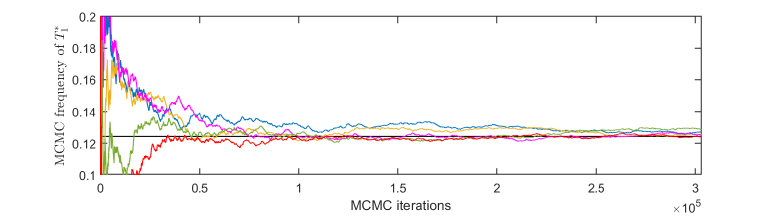
Figure 7: MCMC frequency of $T_{1}^{*}$. The five graphs plotted correspond to five independent repetitions of the experiment with $N=3\times 10^{5}$ iterations; the horizontal line is the limiting frequency, $\pi(T_{1}^{*}|x)$.

Neural spike trains. Next we consider a long binary time series $x$ that consists of $n=3,919,361$ bits, describing the spike train recorded from a single neuron in the V4 region of a monkey’s brain. The recording was made during the experiment described in Gregoriou et al. (2009); Gregoriou et al. (2012), while the monkey was performing an attention task. The recorded signal was discretised into one-millisecond bins (with $x_{i}=1$ if there was a spike in bin $i$ and $x_{i}=0$ otherwise), corresponding to a trial lasting a little over 65 minutes. As we have not been able to find implementations of VLMC or MTD that can operate on data sets of this length, in this section we only present the results obtained by the BCT and $k$-BCT algorithms.

With $D=100$, $\beta=1-2^{-m+1}=1/2$ and $k=5$, the MAP model $T_{1}^{*}$ is shown in Figure 8. It has depth 98 and, with the exception of two additional branches at depths 9 and 90, it is very similar to a renewal model, qualitatively similar to the first chain in Section F.1 of the supplementary material. Its prior probability is $\pi(T_{1}^{*})\approx 3.1\times 10^{-61}$ and its posterior $\pi(T_{1}^{*}|x)\approx 2.1\times 10^{-8}$. Although this probability is small, we note that there are more than $79^{10^{29}}$ possible models of depth no more than 100, cf. (9), and that this posterior is still larger than the corresponding prior probability by more than 50 orders of magnitude. Therefore, the observations $x$ offer significant support for this model.

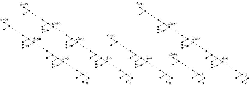
Figure 8: The top $k=5$ models obtained by $k$-BCT on the spike train data. The posterior odds $\pi(T_{1}^{*}|x)/\pi(T_{i}^{*}|x)$ for $i=2,3,4,5$, are $\approx 1.2$, $1.43$, $1.52$ and $1.53$, respectively.

The next four a posteriori most likely models shown in Figure 8 are also very similar to simple renewal models, offering a partial justification to the biological intuition behind the elementary Poisson/renewal models commonly used in neuroscience (Rieke et al., 1999; Dayan and Abbott, 2001), and confirming relevant earlier findings (Gao et al., 2006, 2008). In other words, we have learned from the data that the statistically most significant factor in determining whether a neuron will fire, given its past history, is the time when it most recently fired before.

Although the sum of the posterior probabilities of the top five models is less than $10^{-7}$, in this case it would not make sense to employ an MCMC sampler to explore the posterior further. The reason is that, given the very small values of the posterior probabilities of the top 5 models, even with $10^{6}$ MCMC samples visiting $10^{6}$ distinct models, we would still only visit around $1\%$ of the support of the posterior, at best. On the other hand, increasing the value of $k$ can give a better idea of the shape of the posterior near its mode $T_{1}^{*}$. With $k=50$, $k$-BCT produced 50 trees, all of depth 98, and all of them being small variations of the renewal model $T_{4}^{*}$: All the resulting models $T_{i}^{*}$ had between one and five additional branches at various depths. The sum of their posterior probabilities is $\approx 4.1\times 10^{-7}$.

As a final test of the scalability of the BCT algorithm on a large data set, we obtained the MAP tree with maximum depth $D=1500$. Interestingly, it is the same as the MAP tree for $D=100$, and with only a slightly smaller posterior probability of $\approx 1.6\times 10^{-8}$.

5 Posterior exploration and estimation

We present two examples that illustrate the utility of the MCMC samplers in Section 3.5 for posterior exploration, and the application of the BCT methodology to parameter estimation and Markov order estimation.

Example 5.1 (Daily changes in S&P 500)

We consider the daily changes in Standard & Poor’s index, from January 2, 1928 until October 7, 2016 (available at https://finance.yahoo.com/quote/^GSPC/), quantised to $m=7$ values: If the change between two successive trading days, day $(i-1)$ and day $i$, is smaller than $-3\%$, $x_{i}$ is set equal to 0; for changes in the intervals $(-3\%,-2\%]$, $(-2\%,-1\%]$, $(-1\%,+1\%]$, $(1\%,2\%]$, and $(2\%,3\%],$ $x_{i}$ is set equal to $1,2,3,4$ and 5, respectively; and for changes greater than $3\%$, $x_{i}=6$.

Based on the resulting $n=22900$ points $x_{i}$, the top $k=5$ a posteriori most likely models obtained by the $k$-BCT algorithm with maximum tree depth $D=260$ (corresponding to approximately one calendar year’s trading days), are described in Figure 9.

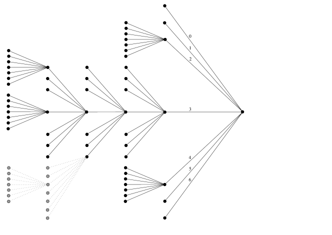
Figure 9: The tree shown without the two dotted branches is the MAP model $T_{1}^{*}$ obtained from $n=22900$ observations, with $D=260$. Its posterior probability $\pi(T_{1}^{*}|x)\approx 0.0174$ and its prior $\pi(T_{1}^{*})\approx 5.7\times 10^{-11}$. The whole tree shown is the fifth a posteriori most likely model $T^{*}_{5}$, and $T_{2}^{*}$, $T_{3}^{*}$ and $T_{4}^{*}$ were found to be small variations around $T_{1}^{*}$ and $T_{5}^{*}$, all with depth 5. The corresponding posterior odds $\pi(T_{1}^{*}|x)/\pi(T_{i}^{*}|x)$, for $i=2,3,4,5$, are $1.094$, $1.367$, $1.496$ and $2.467$, respectively.

The shape of the MAP model $T_{1}^{*}$ contains significant information. Since its maximal depth is 5, in order to determine the distribution of the next sample we never have to look more than five days back – corresponding to a week of trading days. The smaller the changes in the most recent S&P values, the further back we need to look in order to predict tomorrow’s value. For example, if the difference between yesterday and today is larger than $\pm 2\%$, we need look no further than yesterday; if it is between $1\%$ and $2\%$, we need to look at the day before yesterday as well; and if it is smaller than $\pm 1\%$, we need to look even further back, but no more than a week.

The sum of the posterior probabilities of the top $k=5$ models is less than $6.5\%$. But with $n=22900$ data points, $m=7$ and $D=260$, the complexity of $k$-BCT becomes prohibitive for large values of $k$. In order to explore $\pi(T|x)$ further, we ran the RW sampler with $T^{(0)}=T_{1}^{*}$ for $N=10^{6}$ iterations. The acceptance rate was $\approx 44.9\%$, and a total of 356531 different models were visited. The MCMC frequencies of the 25 most visited models shown in Figure 10 indicate that the sampler has converged after $N=10^{6}$ iterations.

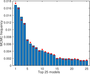
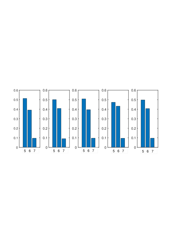
Figure 10: Left: MCMC empirical frequencies of the 25 most frequently visited models, after $N=10^{6}$ iterations. The corresponding true posterior probabilities are marked with a red ‘x’. Right: Markov order estimation: The five histograms show the empirical frequencies of the depths of the 1,000 most visited models after $10^{6}$ MCMC iterations, in five independent repetitions of the same experiment.

The MCMC output can also be used for Markov order estimation, by providing an approximation to the posterior distribution on model depth. The empirical distributions of the model depths obtained in five repetitions of the same experiment are shown in Figure 10.

Example 5.2 (A bimodal posterior)

Consider a 3rd order chain $\{X_{n}\}$ on the alphabet $A=\{0,1,2,3,4,5\}$ with the property that each $X_{n}$ depends on the past $(X_{n-1},X_{n-2},X_{n-3})$ only via $X_{n-3}$. Specifically, suppose that, for $i,j,a,b\in A$,

$$\Pr(X_{n}=j|X_{n-1}=a,X_{n-2}=b,X_{n-3}=i)=Q_{ij},$$

where the transition matrix $Q=(Q_{ij})$ is given in Section E of the supplementary material.

The model of $\{X_{n}\}$ viewed as a variable-memory chain is clearly the complete tree of depth 3, but the dependence of each $X_{n}$ on its past is only meaningful if it can extend at least three time steps back: The first and second most recent symbols are independent of $X_{n}$.

Therefore, it is not surprising that the MAP model identified by the $k$-BCT algorithm (with $k=5$, based on $n=1850$ samples) is simply the root, $T_{1}^{*}=\Lambda=\{\lambda\}$, with $T_{2}^{*}$ a complex tree of depth 3 (with 54 leaves at depth 3) being a close second; their posterior probabilities are $\pi(T_{1}^{*}|x)\approx 0.3512$ and $\pi(T_{1}^{*}|x)\approx 0.2373$, respectively. The next three a posteriori most likely models $T_{3}^{*},T_{4}^{*},T_{5}^{*}$ were found to be small variations of $T_{2}^{*}$, also of depth 3.

Running the RW sampler with $T^{(0)}=T_{1}^{*}$, we found that it never visited any of the other top $5$ models after $10^{6}$ iterations, and similarly starting at $T_{2}^{*}$ it never visited $T_{1}^{*}$. Although $T^{*}_{2}$ can theoretically be reached from $T_{1}^{*}$ in just 12 MCMC steps, most models between them have extremely small posterior probabilities; e.g., the complete tree of depth one, $T_{c}(1)$, which must necessarily be visited in order to move between $T_{1}^{*}$ and $T_{2}^{*}$, has $\pi(T_{c}(1)|x)\approx 3.2\times 10^{-19}$.

In contrast, the jump sampler with jump parameter $p=1/2$, made frequent jumps between $T_{1}^{*}$ and $\{T_{2}^{*},T_{3}^{*},T_{4}^{*},T_{5}^{*}\}$. Starting with $T^{(0)}=T_{1}^{*}$, after $N=10^{5}$ MCMC iterations it appears to have explored the bulk of the posterior distribution, having visited all of the significant parts of its support. The empirical frequencies of the top 5 models were very close to their actual posterior probabilities (Figure 11), the total number of unique models visited was 39, and the sum of their posterior probabilities was $\approx 99.8\%$.

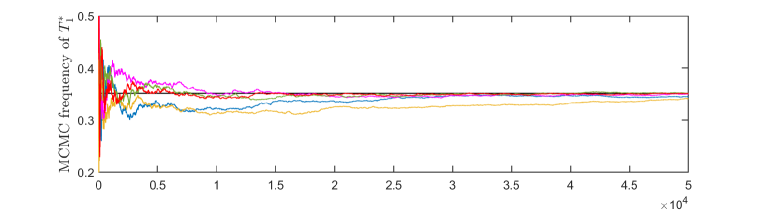
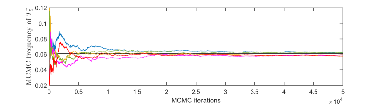
Figure 11: Results of the jump sampler. The top plot shows the empirical frequency with which $T_{1}^{*}$ appears in the MCMC sample, as a function of the number of MCMC iterations. The five graphs plotted correspond to five independent repetitions of the experiment with $50,000$ iterations; the horizontal line is the limiting frequency, $\pi(T_{1}^{*}|x)$. The bottom plot shows corresponding results for $T_{5}^{*}$.

In terms of Markov order estimation, although the MAP model $T_{1}^{*}$ has depth 0, the mode of the posterior distribution of the depth parameter is 3: The $N=10^{5}$ MCMC samples obtained above consist entirely of models having depths either 0 or 3, with corresponding MCMC frequencies of approximately 35.13% and 64.87%, respectively.

More generally, for any statistic $F(\theta,T)$, we can obtain MCMC samples $\{(\theta^{(t)},T^{(t)})\}$ using the joint sampler of Section 3.5, and use the values $\{F(\theta^{(t)},T^{(t)})\}$ to provide an approximation to the posterior $\pi(F|x)$. Standard Bayesian methods (Geisser, 1993; Bernardo and Smith, 1994; Gelman et al., 2014) can then be applied to provide point estimates, credible sets, and other relevant information.

For example, suppose we wish to estimate the parameter $\theta_{s}(j)=\Pr(X_{0}=j|X_{-D}^{-1}=s),$ for the specific context $s=020$ and $j=5$. The maximum likelihood estimate (MLE) is $\hat{\theta}^{\rm MLE}_{s}(j)=a_{s}(j)/M_{s},$ and a commonly used Bayesian counterpart to the MLE, $\hat{\theta}^{\rm MAP}_{s}(j)$, is the mode of the full conditional density $\pi(\theta_{s}(j)|x,T)$ in (20) of $\theta_{s}(j)$ given the data $x$ and the MAP model $T=T_{1}^{*}$. Another Bayesian alternative to the MLE is the posterior mean, which can be approximated as,

$$\hat{\theta}^{\rm MCMC}_{s}(j):=\frac{1}{N}\sum_{t=1}^{N}\theta^{(t)}_{s}(j),$$

and an estimator with smaller variance can also be obtained via Rao-Blackwellization (Gelfand and Smith, 1990), using (20):

$$\hat{\theta}^{\rm RB}_{s}(j):=\frac{1}{N}\sum_{t=1}^{N}E\big{(}\theta_{s}(j)\big{|}x,T^{(t)}\big{)}.$$

In this example, we obtain the values:

$\displaystyle{\hat{\theta}^{\rm MLE}_{s}(j)}$	$\hat{\theta}^{\rm MAP}_{s}(j)$	$\hat{\theta}^{\rm MCMC}_{s}(j)$	$\hat{\theta}^{\rm RB}_{s}(j)$	true $\theta_{s}(j)$
0.1290	0.1871	0.1512	0.1516	0.15

The estimates $\hat{\theta}^{\rm MCMC}_{s}(j)$ and $\hat{\theta}^{\rm RB}_{s}(j)$ are based on $N=10^{5}$ MCMC samples obtained by the jump version of the joint sampler, with jump parameter $p=1/2$. From the same samples we get an estimate of the posterior distribution of $\theta_{020}(5)$, shown in Figure 12.

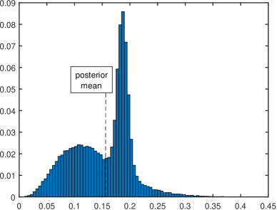
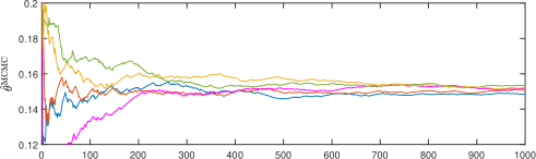
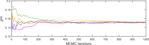
Figure 12: Left: Histogram of the $N=10^{5}$ MCMC samples $\theta^{(t)}_{s}(j)$, with $D=3$, $\beta=0.95$, $s=020$ and $j=5$. Right: Corresponding MCMC estimates. The top plot shows the ergodic averages $\hat{\theta}^{\rm MCMC}_{s}(j)$ as a function of the number of MCMC iterations. The five graphs plotted correspond to five independent repetitions with only $N=1,000$ MCMC iterations each. The bottom plot shows corresponding results for $\hat{\theta}^{\rm RB}_{s}(j)$.

Note that the values of the four estimates above are quite different, which is common, especially for small data sizes $n$. On the other hand, the fact that the Bayesian estimates are more accurate than the MLE is by no means universal.

Finally, in Figure 12 we also show the results of five different MCMC experiments, indicating that the ergodic averages in the estimators $\hat{\theta}^{\rm MCMC}_{s}(j)$ and $\hat{\theta}^{\rm RB}_{s}(j)$ converge quickly, and that the variance of $\hat{\theta}^{\rm RB}_{s}(j)$ appears to be smaller, as expected.

6 Prediction

Given a training sequence $x_{1}^{t}=(x_{1},x_{2},\ldots,x_{t})$ of length $t$ from a discrete time series $x$ with values in the alphabet $A=\{0,1,\ldots,m-1\}$, we wish to sequentially predict the next $n$ values of the test sequence  $x_{t+1}^{t+n}=(x_{t+1},x_{t+2},\ldots,x_{t+n})$. At each step $i=1,2,\ldots,n$, given the past samples $x_{1}^{t+i-1}$, the prediction of the next sample $x_{t+i}$ is expressed as a conditional distribution $\mbox{$\hat{Q}_{i}$}(z|x_{1}^{t+i-1})$, $z\in A$, and the performance of a predictor ${\cal Q}=\{\mbox{$\hat{Q}_{i}$}\;;\;i=1,2,\ldots,n\}$ is evaluated by the normalised, cumulative log-loss.

In the remainder of this section we describe the four prediction methods that will be used below, together with the natural predictor induced by the BCT framework discussed in Section 3.6. In Sections 6.1 and 6.2 we report the results obtained by all five methods on simulated and real data sets, and we discuss them in Section 6.3.

A common approach to prediction is to first use the training data to learn a model and associated parameters, and then use the conditional distributions of this model as predictors. Indeed, this is exactly the form of the predictors proposed by all methods, other than BCT, described below.

Bayesian context trees. As outlined in Section 3.6, the canonical predictor within the BCT framework is the one based on the posterior predictive distribution, $\hat{Q}_{i}(x_{t+i}|x_{1}^{t+i-1})=P^{*}_{D}(x_{i+1}|x_{1}^{i})$, cf. (21), which can easily be computed sequentially via the CTW algorithm. By averaging over all models, $P^{*}_{D}(x_{i+1}|x_{1}^{i})$ incorporates the model uncertainty and it avoids the problem of model selection by replacing it with model averaging.

When the data $x$ are generated by a stationary, irreducible variable-memory chain, in the special case $\beta=1/2$ it is shown by Jiao et al. (2013) that the BCT predictor is consistent with probability one, asymptotically in the size of the test data, for any finite training sequence. Moreover, as the following discussion indicates, the BCT predictor essentially achieves the optimal minimax regret with respect to log-loss. Theorem 6.1 gives a nonasymptotic lower bound, for the special case of binary chains and $\beta=1/2$; it was established in Willems et al. (1993b, 1995).

Theorem 6.1

For any binary, variable-memory chain model $T\in{\cal T}(D)$ and associated parameters $\theta=\{\theta_{s}\;;\;s\in T\}$, for any data sequence $x_{1}^{n}$ of arbitrary length $n$, and any initial context $x_{-D+1}^{0}$, the prior predictive likelihood for $\beta=1/2$ satisfies,

$$\log P_{D}^{*}(x_{1}^{n}|x_{-D+1}^{0})\geq\log P(x_{1}^{n}|x_{-D+1}^{0},\theta,T)-\frac{|T|}{2}\log n+C,$$ (23)

with an explicit constant $C=C(T)$, independent of $n$ and $\theta$.

The lower bound (23) is asymptotically tight up to and including the $\log n$ term, both in expectation and for individual sequences: Corresponding upper bounds follow from the fundamental “converse” theorem by Rissanen (1984, 1986b), and from the general results by Weinberger et al. (1994). These results clearly indicate that the BCT predictor indeed essentially achieves the optimal minimax regret (Takeuchi and Barron, 2014).

Variable length Markov chains. For prediction using variable-length Markov chains we use the prediction function in the R package VLMC. This selects a VLMC model based on the training data, and then predicts future samples by the maximum likelihood parameters associated with this model. Here we only show results for the best-BIC-VLMC model, as it was found to be the most effective choice in practice; see also the relevant comments in Section 4.1. When the data $x$ are generated by a stationary and ergodic variable-memory chain, the results of Bühlmann and Wyner (1999) imply that the VLMC predictor is asymptotically consistent, but for consistency it is the size of the training data that needs to grow to infinity. Further methodology in connection with VLMC prediction is developed in Bühlmann (2000).

Mixture transition distribution. The MTD approach to prediction is again based on first selecting a model and then performing prediction using an approximation to the maximum likelihood parameters associated with that model. Among the four MTD versions discussed in Section 4, we only report results obtained by the best-BIC-MTDg, since the performance of the other three methods was either identical or inferior.

Sparse Markov chains. As described in the Introduction, SMCs are a generalisation of the BCT models in ${\cal T}(D)$: Each SMC model consists of a partition of the set of all contexts of depth $D$ into different states, such that all contexts in the same state induce the same conditional distribution on the next symbol of the underlying chain. In Jääskinen et al. (2014), a class of priors for SMCs are defined, and algorithms for selecting approximate MAP versions of models and parameters are developed in the subsequent work Xiong et al. (2016). In our experiments, prediction is performed based on the resulting model and parameters obtained using the code publicly available at https://www.helsinki.fi/bsg/filer/SMCD.zip.

Conditional tensor factorisation. The CTF models of Sarkar and Dunson (2016), described in the Introduction, use conditional tensor factorisation to represent the full transition probability tensor of a higher-order chain. In our experiments we use the CTF software publicly available at https://github.com/david-dunson/bnphomc. Prediction is again performed in two steps. First a model is selected via the results of an MCMC sampler on model space, and appropriate parameters are chosen by an approximation to their posterior mean via Gibbs sampling. The induced predictive distributions are then obtained from the selected model and parameters.

Throughout our experiments, we take the maximal depth to be $D=10$ for BCT, MTD, SMC and CTF. Following standard practice (Begleiter et al., 2004) in most cases we split the data 50-50 into a training set and a test set. One difficulty that occasionally arises with the VLMC and MTD predictors is that they use maximum likelihood parameter estimates for their models, which in some cases means that they assign zero conditional probability to certain symbols, and which in turn results in poor performance and an infinite log-loss.

Finally we note that different versions of the CTW algorithm have been used for prediction in earlier work, including Ron et al. (1996); Begleiter et al. (2004); Dimitrakakis (2010).

6.1 Simulated data

The experiments here are based on 1,000 samples simulated from the 5th order chain with alphabet size $m=3$ in Section 4.1. Figure 13 shows the log-loss achieved by all five predictors as a function of the number of predicted samples in three different cases.

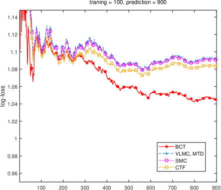
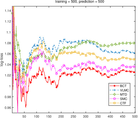
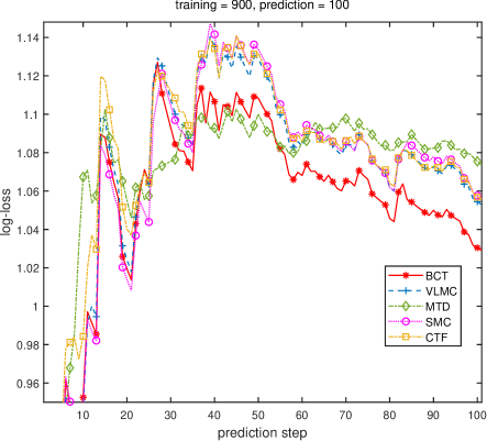
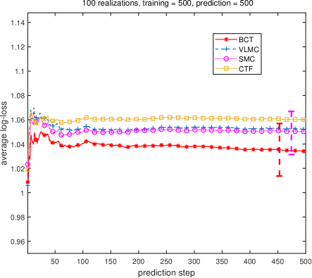
Figure 13: Prediction results on simulated data. First three plots: Log-loss achieved by each of the five methods, as a function of the size of the test data. Bottom right: Log-loss achieved by BCT, VLMC, SMC and CTF on $n=500$ test samples with $t=500$ training samples, averaged over 100 independent repetitions of the same experiment. One-standard-deviation error bars are also plotted for BCT and SMC near the end of the test data. The vertical (log-loss) axis has the same range in all four plots.

The results in the first plot are based on $t=100$ training samples and $n=900$ test samples. The BCT is seen to perform consistently better than the other four methods, and the difference between BCT and the second best method, CTF, increases as more data get predicted, reaching a significant $\approx 3.7\%$ by the end. This is in part due to the fact that the BCT predictor continues to get updated past the training stage, whereas the models employed by the other four methods based on only $100$ training samples are too simple to be effective. SMC, VLMC and MTD all produce the empty model corresponding to i.i.d. data, with VLMC and MTD also having the same parameters, inducing the exact same predictors (hence shown as a single graph). CTF, on the other hand, uses a first order Markov model, leading to slightly better performance.

The second plot shows the log-loss obtained with $t=500$ training samples and $n=500$ test samples. The results are similar, however, the difference between BCT and the other methods is now smaller. Since the training set is larger, the other four methods have a better chance to capture more of the structure present in the data. The VLMC model is a simple tree of depth two, and the CTF model also corresponds to a second order chain. MTD again produces an i.i.d. model, and SMC, which is the closest to BCT, with a log-loss difference of $\approx 2.5\%$, identifies a second order model with five states.

With $t=900$ training and $n=100$ test samples, BCT again appears to have the best performance, although there are larger fluctuations due to the smaller test data size. The results of SMC, VLMC and CTF are almost identical, and significantly better than MTD. SMC uses a second order model with 4 states, the CTF model also has order 2, MTD selects the i.i.d. model, and VLMC, which is closest to BCT by the end (by a 2.2% difference), produces a tree model of depth 3 with 5 leaves.

Finally, we examine the log-loss of these predictors averaged over 100 independent realisations simulated from this chain, each time with a 50-50 split between training and test data. The last plot in Figure 13 shows the results obtained by all methods except MTD, which was based on an i.i.d. model every time. The average performance of BCT is better than that of the other methods; after the first 10 samples or so, the log-loss of the BCT stays consistently approximately 1.6% lower than that of the second best method, SMC.

6.2 Real data

SARS-CoV-2 gene. Here we examine the spike (S) gene, in positions 21,563–25,384 of the SARS-CoV-2 genome (Wu et al., 2020) described in Section 4.2. The importance of this gene is that it codes for the surface glycoprotein whose function was identified in Yan et al. (2020); Lan et al. (2020) as critical, in that it binds onto the Angiotensin Converting Enzyme 2 (ACE2) receptor on human epithelial cells, giving the virus access to the cell and thus facilitating the Covid-19 disease.

The data, consisting of a 3,822 bp-long gene sequence, was again split 50-50 into a training set and test set. Figure 14 shows the prediction results obtained by all five methods. BCT consistently achieves the smallest log-loss. On the training data, the MAP tree produced by BCT corresponds to the full first order Markov model with posterior probability of $\approx 98\%$, while on the entire data set the MAP tree has depth 2. The MAP model $T_{1}^{*}$ now has $\pi(T_{1}^{*}|x)\approx 49.5\%$, while the first order chain which appears as $T_{2}^{*}$ has $\pi(T_{2}^{*}|x)\approx 48\%$. This ability of BCT to perform sequential updates and adaptive model averaging explains, in part, its superior performance.

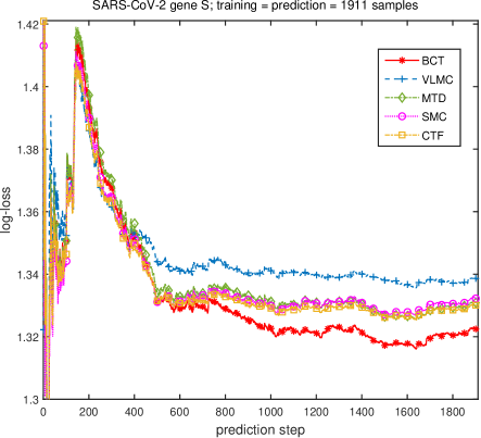
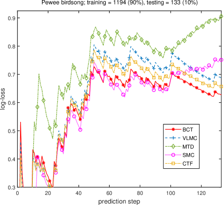
Figure 14: Prediction results on real data. Left: SARS-CoV-2 gene (S), with $t=1911$ training samples and $n=1911$ test samples. Right: Pewee birdsong data, with $t=1194$ training samples and $n=133$ test samples, corresponding to a 90%-training/10%-testing split.

The second best method, CTF, uses a first order Markov model, as does MTD, which achieves near-identical performance. SMC uses a first order model that groups $\{G,T\}$ into a single state, and VLMC similarly produces a tree of depth 1 that groups $\{A,G,T\}$ into a single state.

Pewee birdsong. The data, discussed in Section 4.2, consists of 1,327 samples in a three-letter alphabet. When half of it was used for training and the other half for testing, VLMC and MTD both had an infinite log-loss after the 420th symbol in the test sequence; this was mentioned earlier as a possible drawback of methods that use maximum likelihood estimates for the parameters. Among the methods that give a finite log-loss, BCT was found to have the best performance. SMC produced a second order model with five states, and by the end of the test data its log-loss was larger than that of the BCT by 13.2%. CTF used a fourth order model for prediction, resulting in a log-loss larger than that of BCT by 1.2%.

In order to illustrate the relative performance of all five methods, in Figure 14 we report the prediction results on the last 10% of the samples, after the first 90% have been used for training. The BCT has smallest log-loss overall, approximately 4.8% lower than that of the second best method, CTF, at the end of the experiment. The CTF and MTD predictors both use a fourth order model, SMC finds a second order model with 5 states, and VLMC uses a simple tree model of depth 4.

6.3 Discussion

The BCT predictor was found to have consistently better performance than the other four methods considered, achieving a log-loss that was between 1.2% and 4.8% better than that of the second best method in each case. This is due, in part, to the fact that the BCT predictor is based on averaging over all models and parameters with respect to their posterior distribution, and that it allows for sequential updates beyond the training stage.

The method that performed the closest to BCT in most cases was CTF, which usually identified the same Markov order as the other methods. The VLMC and MTD predictors were found to be consistently and significantly less effective than BCT, and as noted earlier they sometimes assigned zero probability to the occurrence of certain symbols in the data, resulting in an infinite log-loss. Another difficulty with CTF, VLMC and MTD is that they required much more computational effort in the training stage.

The SMC predictor was found in most cases to have performance similar to VLMC. As the context tree models in ${\cal T}(D)$ are a subset of all SMCs, the fact that BCT performs better than SMC highlights the power of the full Bayesian BCT framework. In contrast, SMC uses a single (and often poor) estimate of its MAP model, leading to much less satisfactory results.

7 Concluding remarks

The Bayesian context trees framework introduced in this work was found to be effective for several core statistical tasks in the analysis of discrete time series. Variable-memory Markov chains are a rich class of models that capture important aspects of the higher-order temporal structure naturally present in many types of real-world data, and the associated exact inference algorithms in Sections 3.1–3.3 provide efficient tools for modelling, estimation and prediction. These algorithms, along with the variable-dimensional MCMC samplers of Section 3.5, also facilitate accurate posterior computations that offer a quantitative measure of uncertainty for the estimated models and parameters. The resulting methods were found to outperform several of the most commonly used approaches on both simulated and real-world data.

The exact nature of the algorithms in Sections 3.1–3.3, particularly the ability to compute the prior predictive likelihood, opens the door to numerous other applications that are the object of ongoing work, including anomaly detection, segmentation, and change-point detection. Similarly, the low complexity of the algorithms opens the door to their effective use in problems involving ‘big data’. As has been noted in before connection with VLMCs, the main practical limitation in the application of these tools is when the alphabet size is large.

While our focus has been exclusively on discrete-valued time series, the ideas and techniques introduced in this work can be generalised to real- or vector-valued observations. Important directions of ongoing relevant research include the extension of the exact inference algorithms to various types of tree-structured autoregressive models, and the development of corresponding tools for inference with hidden Bayesian context trees.

Supplementary Material A Proofs of Lemma 2.1 and Theorems 3.1 and 3.2

Throughout this section, for the sake of clarity of notation, we simply write $\pi_{D}(T)$ for the model prior $\pi_{D}(T;\beta)$, without explicit reference to $\beta$.

Proof of Lemma 2.1. The proof is by induction. Note first that for $D=0,1$ the result is trivial to check. Also observe that we can write any tree $T$ which does not contain only the root node $\lambda$, as the union $T=\cup_{j}T_{j}$ of a collection of $m$ subtrees $T_{0},T_{1},\ldots,T_{m-1}$. Clearly we will then have,

$$|T|=\sum_{j}|T_{j}|,\;\;\mbox{and}\;\;L_{D}(T)=\sum_{j}L_{D-1}(T_{j}).$$ (24)

For the inductive step, suppose that the result holds for all depths less than or equal to some $d\leq D-1$. We will show that it holds for $d+1$ as well. Let $\Lambda=\{\lambda\}$ denote the tree that consists only of the root node $\lambda$. Using (24), we have,

$$\sum_{T\in{\cal T}(d+1)}\pi_{d+1}(T) = \pi_{d+1}(\Lambda)+\sum_{T\in{\cal T}(d+1),T\neq\Lambda}\alpha^{|T|-1}\beta^{|T|-L_{d+1}(T)}$$

$$= \beta+\sum_{T_{0},T_{1},\ldots,T_{m-1}\in{\cal T}(d)}\alpha^{\sum_{j}|T_{j}|-1}\beta^{\sum_{j}|T_{j}|-\sum_{j}L_{d}(T_{j})}$$

$$= \beta+\alpha^{m-1}\sum_{T_{0},T_{1},\ldots,T_{m-1}\in{\cal T}(d)}\prod_{j}\alpha^{|T_{j}|-1}\beta^{|T_{j}|-L_{d}(T_{j})}$$

$$= \beta+\alpha^{m-1}\prod_{j}\sum_{T_{j}\in{\cal T}(d)}\pi_{d}(T_{j})$$

$$= \beta+\alpha^{m-1}=1,$$ (26)

where (A) follows by (24), and (26) follows from the inductive hypothesis and the assumption that $\beta=1-\alpha^{m-1}$.     $\Box$

Before giving the proof of Theorem 3.1, we note for later use the following simple properties of the prior $\pi_{D}(T)$. Recall that we write $\Lambda=\{\lambda\}$ for the tree consisting of only the root node $\lambda$.

Lemma A.1

• If $T\in{\cal T}(D)$, $T\neq\Lambda$, is expressed as the union $T=\cup_{j}T_{j}$ of the subtrees $T_{j}\in{\cal T}(D-1)$, then,

  $$\pi_{D}(T)=a^{m-1}\prod_{j=0}^{m-1}\pi_{D-1}(T_{j}),$$ (27)

  where $\alpha^{m-1}=1-\beta$.

• If $T\in{\cal T}(D)$, $t\in T$ is at depth $d<D$, $S\in{\cal T}(D-d)$ is nonempty, and $T\cup S$ consists of the tree $T$ with $S$ added as a subtree rooted at $t$, then,

  $$\pi_{D}(T\cup S)=\beta^{-1}\pi_{D}(T)\pi_{D-d}(S).$$

Proof. The result of $(i)$ immediately follows from the observation (24) in the proof of Lemma 2.1. Similarly, $(ii)$ follows from the simple observations that $|T\cup S|=|T|+|S|-1$ and $L_{D}(T\cup S)=L_{D}(T)+L_{D-d}(S)$, together with the definition of the prior.     $\Box$

Proof of Theorem 3.1. First we note that, without loss of generality, we may assume that the tree $T_{\rm MAX}$ is the complete tree of depth $D$; if some node $s$ of the complete tree is not in $T_{\rm MAX}$, we simply assume that it has an all-zero count vector $a_{s}$.

The proof is again by induction. We adopt the notation of the proof of Lemma 2.1 and observe that, in view of Lemma 2.2, it suffices to show that,

$$P_{w,\lambda}=\sum_{T\in{\cal T}(D)}\pi_{D}(T)\prod_{s\in T}P_{e}(a_{s}).$$ (28)

We claim that the following more general statement holds: For any node $s$ at depth $d$ with $0\leq d\leq D$, we have,

$$P_{w,s}=\sum_{U\in{\cal T}(D-d)}\pi_{D-d}(U)\prod_{u\in U}P_{e}(a_{su}),$$ (29)

where $su$ denotes the concatenation of contexts $s$ and $u$. Clearly (29) implies (28) upon taking $s=\lambda$, and (29) is trivially true for nodes $s$ at depth $D$, since it reduces to the fact that $P_{w,s}=P_{e,s}$ for leaves $s$, by definition.

Suppose (29) holds for all nodes $s$ at depth $d$ for some fixed $0<d\leq D$. Let $s$ be a node at depth $d-1$; then, by the inductive hypothesis,

$$P_{w,s} = \beta P_{e}(a_{s})+(1-\beta)\prod_{j=0}^{m-1}P_{w,sj}$$

$$= \beta P_{e}(a_{s})+(1-\beta)\prod_{j=0}^{m-1}\left[\sum_{T_{j}\in{\cal T}(D-d)}\pi_{D-d}(T_{j})\prod_{t\in T_{j}}P_{e}(a_{sjt})\right],$$

where $sjt$ denotes the concatenation of context $s$, then symbol $j$, then context $t$, in that order. Therefore,

$$P_{w,s} = \beta P_{e}(a_{s})+(1-\beta)\sum_{T_{0},T_{1},\ldots,T_{m-1}\in{\cal T}(D-d)}\prod_{j=0}^{m-1}\left[\pi_{D-d}(T_{j})\prod_{t\in T_{j}}P_{e}(a_{sjt})\right]$$

$$= \beta P_{e}(a_{s})+\frac{1-\beta}{\alpha^{m-1}}\sum_{T_{0},T_{1},\ldots,T_{m-1}\in{\cal T}(D-d)}\pi_{D-d+1}(\cup_{j}T_{j})\left[\prod_{j=0}^{m-1}\prod_{t\in T_{j}}P_{e}(a_{sjt})\right],$$

where for the last step we have used (27) from Lemma A.1. Concatenating every symbol $j$ with every leaf of the corresponding tree $T_{j}$, we end up with all the leaves of the larger tree $\cup_{j}T_{j}$. Therefore,

$$P_{w,s} = \beta P_{e}(a_{s})+\frac{1-\beta}{\alpha^{m-1}}\sum_{T_{0},T_{1},\ldots,T_{m-1}\in{\cal T}(D-d)}\pi_{D-d+1}(\cup_{j}T_{j})\prod_{t\in\cup_{j}T_{j}}P_{e}(a_{st}),$$

and since $1-\beta=\alpha^{m-1}$ and $\pi_{d}(\Lambda)=\beta$ for all $d\geq 1$,

$$P_{w,s} = \pi_{D-d+1}(\Lambda)P_{e}(a_{s})+\sum_{T_{0},T_{1},\ldots,T_{m-1}\in{\cal T}(D-d)}\pi_{D-d+1}(\cup_{j}T_{j})\prod_{t\in\cup_{j}T_{j}}P_{e}(a_{st})$$

$$= \pi_{D-d+1}(\Lambda)P_{e}(a_{s})+\sum_{T\in{\cal T}(D-d+1),T\neq\Lambda}\pi_{D-d+1}(T)\prod_{t\in T}P_{e}(a_{st})$$

$$= \sum_{T\in{\cal T}(D-d+1)}\pi_{D-d+1}(T)\prod_{t\in T}P_{e}(a_{st}).$$

This establishes (29) for all nodes $s$ at depth $d-1$, completing the inductive step and the proof of the theorem.     $\Box$

Proof of Theorem 3.2. Again we observe that, without loss of generality, we may assume that the tree $T_{\rm MAX}$ is the complete tree of depth $D$; if some node $s$ of the complete tree is not in $T_{\rm MAX}$, we simply assume that it has an all-zero count vector $a_{s}$. It is easy to see that, for $\beta\geq 1/2$, these assumptions are equivalent to the ones in the description of the algorithm, giving the same initial values to all leaves of $T_{\rm MAX}$.

The proof is once again by induction, and we adopt the same notation as in the proofs of Lemma 2.1 and Theorem 3.1. First we will prove that,

$$P_{m,\lambda}=\max_{T\in{\cal T}(D)}P(x,T),$$ (30)

which, in view of Lemma 2.2, is equivalent to,

$$P_{m,\lambda}=\max_{T\in{\cal T}(D)}\pi_{D}(T)\prod_{s\in T}P_{e}(a_{s}).$$ (31)

As in the proof of Theorem 3.1, we claim that the following more general statement holds: For any node $s$ at depth $d$ with $0\leq d\leq D$, we have,

$$P_{m,s}=\max_{U\in{\cal T}(D-d)}\pi_{D-d}(U)\prod_{u\in U}P_{e}(a_{su}),$$ (32)

where $su$ denotes the concatenation of contexts $s$ and $u$. Taking $s=\lambda$ in (32) gives (31), and (32) is trivially true for nodes $s$ at depth $D$, since it reduces to the fact that $P_{m,s}=P_{e,s}$ for leaves $s$, by definition.

For the inductive step, we assume that (32) holds for all nodes $s$ at depth $d$ for some fixed $0<d\leq D$, and consider a node $s$ at depth $d-1$. By the inductive hypothesis we have,

$$P_{m,s} = \max\left\{\beta P_{e}(a_{s}),(1-\beta)\prod_{j=0}^{m-1}P_{m,sj}\right\}$$

$$= \max\left\{\beta P_{e}(a_{s}),(1-\beta)\prod_{j=0}^{m-1}\left[\max_{T_{j}\in{\cal T}(D-d)}\pi_{D-d}(T_{j})\prod_{t\in T_{j}}P_{e}(a_{sjt})\right]\right\}$$

$$= \max\left\{\beta P_{e}(a_{s}),(1-\beta)\max_{T_{0},T_{1},\ldots,T_{m-1}\in{\cal T}(D-d)}\prod_{j=0}^{m-1}\left[\pi_{D-d}(T_{j})\prod_{t\in T_{j}}P_{e}(a_{sjt})\right]\right\}$$

$$= \max\left\{\beta P_{e}(a_{s}),\frac{1-\beta}{\alpha^{m-1}}\max_{T_{0},T_{1},\ldots,T_{m-1}\in{\cal T}(D-d)}\pi_{D-d+1}(\cup_{j}T_{j})\left[\prod_{j=0}^{m-1}\prod_{t\in T_{j}}P_{e}(a_{sjt})\right]\right\},$$

where the last step follows by (27) from Lemma A.1. Arguing as in the proof of Theorem 3.1,

$$P_{m,s} = \max\left\{\pi_{D-d+1}(\Lambda)P_{e}(a_{s}),\max_{T_{0},T_{1},\ldots,T_{m-1}\in{\cal T}(D-d)}\pi_{D-d+1}(\cup_{j}T_{j})\prod_{t\in\cup_{j}T_{j}}P_{e}(a_{st})\right\}$$

$$= \max\left\{\pi_{D-d+1}(\Lambda)P_{e}(a_{s}),\max_{T\in{\cal T}(D-d+1),T\neq\Lambda}\pi_{D-d+1}(T)\prod_{t\in T}P_{e}(a_{st})\right\}$$

$$= \max_{T\in{\cal T}(D-d+1)}\pi_{D-d+1}(T)\prod_{t\in T}P_{e}(a_{st}).$$

This establishes (32) for all nodes $s$ at depth $d-1$, completing the inductive step and hence also proving (30) and (31).

To complete the proof of the theorem, it now suffices to show that,

$$P_{m,\lambda}=P(x,T^{*}_{1}),$$ (33)

because this is exactly (16), and combined with (30) it implies,

$$\max_{T\in{\cal T}(D)}P(x,T)=P(x,T^{*}_{1}),$$

which, after dividing both sides by the prior predictive likelihood, $P^{*}_{D}(x)$, gives (15). By Lemma 2.2, (33) is equivalent to,

$$P_{m,\lambda}=\pi_{D}(T^{*}_{1})\prod_{s\in T^{*}_{1}}P_{e}(a_{s}),$$ (34)

and, once again, we will establish the following more general statement: For any node $s$ at depth $d$ with $0\leq d\leq D$, we have,

$$P_{m,s}=\max\Big{\{}\beta P_{e}(a_{s}),(1-\beta)\prod_{j=0}^{m-1}P_{m,sj}\Big{\}}=\pi_{D-d}(T(s))\prod_{t\in T(s)}P_{e}(a_{st}),$$ (35)

where $T(s)$ is the tree that the BCT algorithm would produce if it started its step $(iii)$ at node $s$. Taking $s=\lambda$ in (35) gives (34), and (35) is again trivially true for leaves $s$ at depth $D$, by the definition of the maximal probabilities $P_{m,s}$.

Finally, for the inductive step, suppose (35) holds for all nodes at depth $0<d\leq D$, and let $s$ be a node at depth $d-1$. We consider two separate cases: $(i)$ If the maximum in (35) is achieved by the first term, then $P_{m,s}=\beta P_{e,s}$ and $T(s)$ consists of $s$ only, so that (35) holds trivially; $(ii)$ If the maximum in (35) is achieved by the second term, then $T(s)=\cup_{j}T(sj)$, and using (27) from Lemma A.1 and the inductive hypothesis, we obtain:

$$P_{m,s} = (1-\beta)\prod_{j=0}^{m-1}P_{m,sj}$$

$$= (1-\beta)\prod_{j=0}^{m-1}\left[\pi_{D-d}(T(sj))\prod_{t\in T(sj)}P_{e}(a_{sjt})\right]$$

$$= \pi_{D-d+1}(\cup_{j}T(sj))\prod_{j=0}^{m-1}\prod_{t\in T(sj)}P_{e}(a_{sjt})$$

$$= \pi_{D-d+1}(\cup_{j}T(sj))\prod_{t\in\cup_{j}T(sj)}P_{e}(a_{st})$$

$$= \pi_{D-d+1}(T(s))\prod_{t\in T(s)}P_{e}(a_{st}).$$

This establishes (35) and completes the proof of the theorem.     $\Box$

Supplementary Material B The actual k-BCT algorithm

Here we describe a practical version of the algorithm, which only differs from the idealised version of Section 3.3 in the initialisation step of the maximal probabilities and the position vectors at the leaves of depth $d<D$. After describing the algorithm, we also make some comments on its implementation complexity.

1. Initially, perform two preprocessing steps:

   1. Execute the first two steps $(i)$ and $(ii)$ of the idealised $k$-BCT algorithm on the complete $m$-ary tree of depth $D$, with all the count vectors $a_{s}$ assumed to be equal to zero, $a_{s}=(0,0,\ldots,0)$ for all $s$. Since all nodes at the same depth are identical, this process can be carried out effectively, by performing the relevant computations only at a single node (instead of all $m^{d}$ nodes) for each depth $0\leq d\leq D$.

   2. Build the tree $T_{\rm MAX}$ from the contexts of $x_{-D+1}^{n}$ and compute the count vectors $a_{s}$ and the probabilities $P_{e,s}=P_{e}(a_{s})$ at all nodes $s$ of $T_{\rm MAX}$, as in steps $(i)$–$(iii)$ of CTW.

2. Starting at the leaves and proceeding towards the root, at each node $s$ we compute a list of $k$ maximal probabilities $P_{m,s}^{(i)}$ and $k$ position vectors $c^{(i)}_{s}=(c^{(i)}_{s}(0),c^{(i)}_{s}(1),\ldots,c^{(i)}_{s}(m-1))$, for $i=1,2,\ldots,k$, recursively as follows.

   1. At each leaf $s$ at depth $D$, with a nonzero count vector $a_{s}$, let $P^{(1)}_{m,s}=P_{e,s}$ and $c_{s}^{(1)}=(0,0,\ldots,0)$. For $i=2,3,\ldots,k$, we leave $P^{(i)}$ and $c_{s}^{(i)}$ undefined.

   2. Similarly, at each leaf $s$ at depth $D$, with an all-zero count vector $a_{s}$, let $P^{(1)}_{m,s}=P_{e,s}=1$, $c_{s}^{(1)}=(0,0,\ldots,0)$, and for $i=2,3,\ldots,k$, leave $P^{(i)}$ and $c_{s}^{(i)}$ undefined.

   3. At each leaf $s$ at depth $d<D$, we let the list of the maximal probabilities $P_{m,s}^{(i)}$ and position vectors $c_{s}^{(i)}$ of $s$ be those that are computed for a node at depth $d$ in the preprocessing stage $(ia)$.

   4. Continue with steps $(iib)$ and $(iic)$ as in the idealised version of $k$-BCT.

3. We perform the same steps as described in $(iiia)$–$(iiid)$ of the idealised version, with the following addition:

   1. While examining a node $s$ at depth $0<d<D$ in step $(iiib)$ or $(iiic)$ of the idealised algorithm, we may reach a point where the algorithm dictates that we examine its $m$ children, when these children are not included in the tree $T_{\rm MAX}$. In that case, we add them to $T_{\rm MAX}$, and we define their corresponding maximal probabilities and position vectors according to the initialisation described in step $(iib)$ or $(iic)$ above, depending on whether $d=D-1$ or $d<D-1$, respectively.

4. As in the idealised version, output the $k$ resulting trees $T^{*}_{i}$ and the $k$ maximal probabilities at the root, $P^{(i)}_{m,\lambda}$, $i=1,2,\ldots,k$.

Complexity of $k$-BCT. As discussed in Sections 1.1 and 3.6 of the main text, the complexity of the $k$-BCT algorithm in its most naive implementation is $O(nmD\times k^{m})$. The factor $k^{m}$ comes from step $(iic)$ of the idealized algorithm, where for every internal node $s$, all possible combinations from the $m$ lists of probabilities $P_{m,sj}$ are computed. However, the fact that these lists $P_{m,sj}$ are already ordered means that the top-$k$ combinations can be found more efficiently, without performing an exhaustive search over all combinations. In particular, a best-first search can be employed to find only the top-$k$ combinations: A priority queue can be used to maintain all possible candidates and efficiently pick the next best. This reduces the complexity to $O\left(nmD\times km\log(km)\right)$.

Supplementary Material C Proof of Theorem 3.3

Before giving the proof of Theorem 3.3, we observe that it is easy (though somewhat tedious) to verify that the two versions of the $k$-BCT algorithm described in Section B are equivalent, in that they produce identical results as long as $\beta\geq 1/2$. Therefore, for the sake of simplicity, the proof below is given only for the idealised $k$-BCT algorithm.

We adopt the same notation as in Section A.

Proof of Theorem 3.3. The proof is again by induction, and we adopt the same notation as in the proof of Theorem 3.2. First we will prove that, for all $1\leq i\leq k$,

$$P^{(i)}_{m,\lambda}=\mathop{{\rm max}^{(i)}}_{T\in{\cal T}(D)}P(x,T),$$ (36)

which, in view of Lemma 2.2, is equivalent to,

$$P^{(i)}_{m,\lambda}=\mathop{{\rm max}^{(i)}}_{T\in{\cal T}(D)}\pi_{D}(T)\prod_{s\in T}P_{e}(a_{s}).$$ (37)

As in the proof of Theorem 3.2, we claim that the following more general statement holds: For all $i$ and any node $s$ at depth $d$ with $0\leq d\leq D$, we have,

$$P^{(i)}_{m,s}=\mathop{{\rm max}^{(i)}}_{U\in{\cal T}(D-d)}\pi_{D-d}(U)\prod_{u\in U}P_{e}(a_{su}),$$ (38)

where $su$ denotes the concatenation of contexts $s$ and $u$. Taking $s=\lambda$ in (38) gives (37), and (38) is trivially true for nodes $s$ at depth $D$, since at depth $D$ we only consider $i=1$ and then $P^{(1)}_{m,s}=P_{e,s}$ for leaves $s$, by definition.

For the inductive step, we assume that (38) holds for all $i$ and all nodes $s$ at depth $d$ for some fixed $0<d\leq D$, and consider a node $s$ at depth $d-1$. By the inductive hypothesis we have, in the notation of (17), that $P^{(i)}_{m,s}$ is equal to,

$$\mathop{{\rm max}^{(i)}}\left[\bigcup_{i_{0}=1}^{k_{0}}\bigcup_{i_{1}=1}^{k_{1}}\cdots\bigcup_{i_{m-1}=1}^{k_{m-1}}\left\{(1-\beta)\prod_{j=0}^{m-1}P^{(i_{j})}_{m,sj}\right\}\bigcup\,\big{\{}\beta P_{e}(a_{s})\big{\}}\right]$$

$$= \mathop{{\rm max}^{(i)}}\left[\bigcup_{i_{0}=1}^{k_{0}}\bigcup_{i_{1}=1}^{k_{1}}\cdots\bigcup_{i_{m-1}=1}^{k_{m-1}}\left\{(1-\beta)\prod_{j=0}^{m-1}\left[\mathop{{\rm max}^{(i_{j})}}_{T_{j}\in{\cal T}(D-d)}\pi_{D-d}(T_{j})\prod_{t\in T_{j}}P_{e}(a_{sjt})\right]\right\}\bigcup\,\big{\{}\beta P_{e}(a_{s})\big{\}}\right]$$

$$= \mathop{{\rm max}^{(i)}}\left[\bigcup_{i_{0}=1}^{k_{0}}\bigcup_{i_{1}=1}^{k_{1}}\cdots\bigcup_{i_{m-1}=1}^{k_{m-1}}\right.$$

$$\hskip 43.36243pt\left\{(1-\beta)\mathop{{\rm max}^{(i_{0})}}_{T_{0}\in{\cal T}(D-d)}\mathop{{\rm max}^{(i_{1})}}_{T_{1}\in{\cal T}(D-d)}\cdots\mathop{{\rm max}^{(i_{m-1})}}_{T_{m-1}\in{\cal T}(D-d)}\prod_{j=0}^{m-1}\left[\pi_{D-d}(T_{j})\prod_{t\in T_{j}}P_{e}(a_{sjt})\right]\right\}$$

$$\hskip 65.04256pt\bigcup\,\big{\{}\beta P_{e}(a_{s})\big{\}}\Bigg{]}$$

$$= \mathop{{\rm max}^{(i)}}\left[\bigcup_{i_{0}=1}^{k_{0}}\bigcup_{i_{1}=1}^{k_{1}}\cdots\bigcup_{i_{m-1}=1}^{k_{m-1}}\right.$$

$$\hskip 43.36243pt\left\{\mathop{{\rm max}^{(i_{0})}}_{T_{0}\in{\cal T}(D-d)}\mathop{{\rm max}^{(i_{1})}}_{T_{1}\in{\cal T}(D-d)}\cdots\mathop{{\rm max}^{(i_{m-1})}}_{T_{m-1}\in{\cal T}(D-d)}\pi_{D-d+1}(\cup_{j}T_{j})\left[\prod_{j=0}^{m-1}\prod_{t\in T_{j}}P_{e}(a_{sjt})\right]\right\}$$

$$\hskip 65.04256pt\bigcup\,\big{\{}\beta P_{e}(a_{s})\big{\}}\Bigg{]},$$

where the last step follows by (27) from Lemma A.1. Therefore, $P^{(i)}_{m,s}$ is equal to,

$$\mathop{{\rm max}^{(i)}}\left[\bigcup_{i_{0}=1}^{k_{0}}\bigcup_{i_{1}=1}^{k_{1}}\cdots\bigcup_{i_{m-1}=1}^{k_{m-1}}\left\{\mathop{{\rm max}^{(i_{0})}}_{T_{0}\in{\cal T}(D-d)}\cdots\mathop{{\rm max}^{(i_{m-1})}}_{T_{m-1}\in{\cal T}(D-d)}\pi_{D-d+1}(\cup_{j}T_{j})\prod_{t\in\cup_{j}T_{j}}P_{e}(a_{st})\right\}\right.$$

$$\hskip 65.04256pt\bigcup\big{\{}\pi_{D-d+1}(\Lambda)P_{e}(a_{s})\big{\}}\Bigg{]}$$

$$= \mathop{{\rm max}^{(i)}}\left[\bigcup_{i^{\prime}=1}^{k}\left\{\mathop{{\rm max}^{(i^{\prime})}}_{T\in{\cal T}(D-d+1),T\neq\Lambda}\pi_{D-d+1}(T)\prod_{t\in T}P_{e}(a_{st})\right\}\bigcup\big{\{}\pi_{D-d+1}(\Lambda)P_{e}(a_{s})\big{\}}\right]$$

$$= \mathop{{\rm max}^{(i)}}_{T\in{\cal T}(D-d+1)}\pi_{D-d+1}(T)\prod_{t\in T}P_{e}(a_{st}).$$

This establishes (38) for all $i$ and all nodes $s$ at depth $d-1$, completing the inductive step and hence also proving (36) and (37).

To complete the proof of the theorem, it now suffices to show that, for all $1\leq i\leq k$,

$$P^{(i)}_{m,\lambda}=P(x,T^{*}_{i}),$$ (39)

because, combined with (36) this implies,

$$\mathop{{\rm max}^{(i)}}_{T\in{\cal T}(D)}P(x,T)=P(x,T^{*}_{i}),$$

which, after dividing both sides by the prior predictive likelihood, gives (18). By Lemma 2.2, (39) is equivalent to,

$$P^{(i)}_{m,\lambda}=\pi_{D}(T^{*}_{i})\prod_{s\in T^{*}_{i}}P_{e}(a_{st}),$$ (40)

and, once again, we will establish the following more general statement: For all $i$ and any node $s$ at depth $d$ with $0\leq d\leq D$, we have,

$$P^{(i)}_{m,s} = \mathop{{\rm max}^{(i)}}\left[\bigcup_{i_{0}=1}^{k_{0}}\bigcup_{i_{1}=1}^{k_{1}}\cdots\bigcup_{i_{m-1}=1}^{k_{m-1}}\left\{(1-\beta)\prod_{j=0}^{m-1}P^{(i_{j})}_{m,sj}\right\}\bigcup\,\big{\{}\beta P_{e}(a_{s})\big{\}}\right]$$ (41)

$$= \pi_{D-d}(T^{(i)}(s))\prod_{t\in T^{(i)}(s)}P_{e}(a_{st}),$$ (42)

where $T^{(i)}(s)$ is the $i$th tree that $k$-BCT would produce if it started its step $(iii)$ at node $s$. Taking $s=\lambda$ in (42) gives (40), and (42) is again trivially true for leaves $s$ at depth $D$, by the definition of the maximal probabilities $P_{m,s}$.

Finally, for the inductive step assume (42) holds for all nodes at depth $0<d\leq D$, and let $s$ be a node at at depth $d-1$. We consider two separate cases: $(i)$ If the maximum in (41) is achieved by the last term, then $P^{(i)}_{m,s}=\beta P_{e,s}$ and $T^{(i)}(s)$ consists of $s$ only, so that (42) holds trivially; $(ii)$ If the maximum in (41) is achieved by the collection of indices $(i_{0},i_{1},\ldots,i_{m-1})$, then $T^{(i)}(s)=\cup_{j}T^{(i_{j})}(sj)$, and using (27) from Lemma A.1 and the inductive hypothesis, we obtain:

$$P^{(i)}_{m,s} = (1-\beta)\prod_{j=0}^{m-1}P^{(i_{j})}_{m,sj}(a_{sj})$$

$$= (1-\beta)\prod_{j=0}^{m-1}\left[\pi_{D-d}(T^{(i_{j})}(sj))\prod_{t\in T^{(i_{j})}(sj)}P_{e}(a_{sjt})\right]$$

$$= \pi_{D-d+1}(\cup_{j}T^{(i_{j})}(sj))\prod_{j=0}^{m-1}\prod_{t\in T^{(i_{j})}(sj)}P_{e}(a_{sjt})$$

$$= \pi_{D-d+1}(\cup_{j}T^{(i_{j})}(sj))\prod_{t\in\cup_{j}T^{(i_{j})}(sj)}P_{e}(a_{st})$$

$$= \pi_{D-d+1}(T^{(i)}(s))\prod_{t\in T^{(i)}(s)}P_{e}(a_{st}).$$

This establishes (42) and completes the proof of the theorem.     $\Box$

Supplementary Material D Arbitrary Dirichlet parameters

In some cases it may be desirable to consider a more general Dirichlet prior $\pi(\theta|T)$ on the parameters $\theta$ associated with a given model $T\in{\cal T}(D)$. Instead of the Dir$(1/2,1/2,\ldots,1/2)$ distribution defined in (6) we may place a different, general Dir$(\gamma_{s}(0),\gamma_{s}(1),\ldots,\gamma_{s}(m-1))$ prior on each context $s\in T$.

For an arbitrary collection of hyperparameters $\gamma=\{\gamma_{s}=(\gamma_{s}(0),\ldots,\gamma_{s}(m-1))\;;\;s\in T\},$ with each $\gamma_{s}(j)>0$, let $\pi(\theta|T)=\prod_{s\in T}\pi(\theta_{s})$, with,

$$\pi(\theta_{s})=\pi(\theta_{s}(0),\theta_{s}(1),\ldots,\theta_{s}(m-1))=\frac{\Gamma(M^{\prime}_{s})}{\prod_{j=0}^{m-1}\Gamma(\gamma_{s}(j))}\prod_{j=0}^{m-1}\theta_{s}(j)^{\gamma_{s}(j)-1}\propto\prod_{j=0}^{m-1}\theta_{s}(j)^{\gamma_{s}(j)-1},$$

where $M^{\prime}_{s}:=\sum_{j=0}^{m-1}\gamma_{s}(j)$, $s\in T$.

As in Section 2.3, the marginal likelihood $P(x|T)$ of a data string $x$ given a model $T\in{\cal T}(D)$ can be computed explicitly. Lemma D.1 below is the analog of Lemma 2.2 in this case.

Lemma D.1

The marginal likelihood $P(x|T)$ of the observations $x$ given a model $T$ is,

$$P(x|T)=\int P(x,\theta|T)d\theta=\int P(x|\theta,T)\pi(\theta|T)d\theta=\prod_{s\in T}P_{e}(a_{s},\gamma_{s}),$$

where the count vectors $a_{s}=(a_{s}(0),a_{s}(1),\ldots,a_{s}(m-1))$ are defined in (4) as before and the estimated probabilities $P_{e}(a_{s},\gamma_{s})$ are now defined by,

$$P_{e}(a_{s},\gamma_{s}):=\frac{\Gamma(M^{\prime}_{s})}{\Gamma(M_{s}+M^{\prime}_{s})}\prod_{j=0}^{m-1}\frac{\Gamma(a_{s}(j)+\gamma_{s}(j))}{\Gamma(\gamma_{s}(j))},$$ (43)

where $M_{s}:=a_{s}(0)+a_{s}(1)+\cdots+a_{s}(m-1)$ and $M^{\prime}_{s}:=\gamma_{s}(0)+\gamma_{s}(1)+\cdots+\gamma_{s}(m-1)$, again with the convention that any empty product is taken to be equal to 1.

Now it is straightforward to modify the CTW, BCT and $k$-BCT algorithms, simply by replacing the estimated probabilities $P_{e}(a_{s})$ of (8) by $P_{e}(a_{s},\gamma_{s})$ as in (43). A careful inspection of the proofs of Theorems 3.1, 3.2 and 3.3 shows that their results remain valid in this more general case.

Corollary D.2

Suppose that, for each model $T\in{\cal T}(D)$, the prior $\pi(\theta|T)$ on the parameters $\theta=\{\theta_{s}\;;\;s\in T\}$ is the product of Dir$(\gamma_{s}(0),\gamma_{s}(1),\ldots,\gamma_{s}(m-1))$ distributions, for an arbitrary collection of hyperparameters $\gamma$. If the estimated probabilities $P_{e}(a_{s})$ of (8) are replaced by $P_{e}(a_{s},\gamma_{s})$ as in (43) in the CTW, BCT and $k$-BCT algorithms, then the results of Theorems 3.1, 3.2 and 3.3 remain valid exactly as stated.

Similarly, all of the additional results in Section 3.4 remain valid as stated there, with the exception of the expression for the full conditional density in (20). In the case of a general prior $\pi(\theta|T)$ in terms of the hyperparameters $\gamma$, the same computation shows that here:

$$\pi(\theta|T,x)=\prod_{s\in T}\text{Dir}\big{(}a_{s}(0)+\gamma_{s}(0),\ldots,a_{s}(m-1)+\gamma_{s}(m-1)\big{)}.$$

Finally, we note that sequential updates, as outlined in Section 3.6, can be carried out for the CTW, BCT, and $k$-BCT algorithms in this more general setting as well. The only change is in the computation required to update $P_{e}(a_{s})$ in step $(iii^{\prime})$, where, in the general case, $P_{e}(a_{s},\gamma_{s})$ is updated by multiplying its earlier value by,

$$\frac{a_{s}(j)+\gamma_{s}(j)-1}{M_{s}^{\prime}+M_{s}-1},$$

using the updated values of $a_{s}$ and $M_{s}$.

Supplementary Material E Explicit computations and numerical values

In this section we give more details on some expressions and explicit numerical values that are omitted in the main text.

RW sampler. The ratios $r(T,T^{\prime})$ in the acceptance probabilities of the RW sampler in Section 3.5 are given by,

$$r(T,T^{\prime}):=\frac{\pi(T^{\prime}|x)}{\pi(T|x)}\times\begin{cases}1/2,&\mbox{in case (a)};\\ m^{D-1}/2,&\mbox{in case (b)};\\ (|T|-L_{D}(T))/N_{D}(T^{\prime}),&\mbox{in case (c), if $T^{\prime}\neq T_{c}(D)$};\\ 2m^{-D+1},&\mbox{in case (c), if $T^{\prime}=T_{c}(D)$};\\ N_{D}(T)/(|T^{\prime}|-L_{D}(T^{\prime})),&\mbox{in case (d), if $T^{\prime}\neq\Lambda$};\\ 2,&\mbox{in case (d), if $T^{\prime}=\Lambda$},\end{cases}$$

where $N_{D}(T)$ denotes the number of internal nodes in a tree $T$ having only $m$ descendants, and the posterior odds $\pi(T^{\prime}|x)/\pi(T|x)$ can be computed via (19).

Jump sampler. The jump sampler of Section 3.5 incorporates the RW sampler’s proposal distribution as one of its steps: Let $q(T^{\prime}|T)$ denote the proposal probabilities of the RW sampler, so that $q(T^{\prime}|T)$ equals 1, $m^{-D+1}$, $1/[2(|T|-L_{D}(T))]$ and $1/[2N_{D}(T)]$, in each of its cases $(ia)$, $(ib)$, $(ic)$ and $(id)$, respectively. We say that two models $T,T^{\prime}$ are neighbours if they differ by exactly one branch of $m$ children.

The ratios $r(T,T^{\prime})$ in the acceptance probabilities of the jump sampler are given by,

$$r(T,T^{\prime}):=\frac{\pi(T^{\prime}|x)}{\pi(T|x)}\times\begin{cases}\frac{(1-p)q(T|T^{\prime})+pk^{-1}{\mathbb{I}}\{T\in{\cal T}^{*}\}}{(1-p)q(T^{\prime}|T)+pk^{-1}{\mathbb{I}}\{T^{\prime}\in{\cal T}^{*}\}},&\;\;\;\mbox{if $T,T^{\prime}$ are neighbours},\\ {\mathbb{I}}\{T\in{\cal T}^{*}\},&\;\;\;\mbox{if $T,T^{\prime}$ are not neighbours},\end{cases}$$

where ${\mathbb{I}}\{\cdot\}$ denotes the indicator function of the event $\{\cdot\}$.

Parameter values. The transition matrix $Q=(Q_{ij})$ in Example 5.2 is:

$$\left(\begin{array}[]{cccccc}0.5&0.2&0.1&0&0.05&0.15\\ 0.4&0&0.4&0.2&0&0\\ 0.3&0.1&0.23&0.12&0.05&0.2\\ 0.05&0.1&0.05&0.05&0.03&0.72\\ 0&0&1&0&0&0\\ 0.1&0.2&0.3&0.2&0.05&0.15\\ \end{array}\right).$$

The parameter vector $\theta=(\theta_{s})$ of the 5th order chain in Section 4.1 is given by:

$$\theta_{1}=(0.4,0.4,0.2),\;\theta_{2}=(0.2,0.4,0.4),$$

$$\theta_{00}=(0.4,0.2,0.4),\;\theta_{01}=(0.3,0.6,0.1),$$

$$\theta_{022}=(0.5,0.3,0.2),$$

$$\theta_{0212}=(0.1,0.3,0.6),\;\theta_{0211}=(0.05,0.25,0.7),\;\theta_{0210}=(0.35,0.55,0.1),$$

$$\theta_{0202}=(0.1,0.2,0.7),\;\theta_{0201}=(0.8,0.05,0.15),$$

$$\theta_{02002}=(0.7,0.2,0.1),\;\theta_{02001}=(0.1,0.1,0.8),\;\theta_{02000}=(0.3,0.45,0.25).$$

Supplementary Material F Model selection examples

F.1 Simulated data

Renewal process. The binary variable-memory chain $\{X_{n}\}$ with model and parameters shown in Figure 15 was examined in the VLMC work of (Bühlmann, 2000, p. 303). Note that the distribution of the next symbol produced by the chain only depends on how far in the past the most recent “0” appeared.

Figure 15: The model and parameters of the renewal-like binary chain.

$\bullet\;\;n=200$. With $n=200$ samples $x$, the BCT algorithm with $D=10$ and $\beta=1-2^{-m+1}=1/2$ produces a MAP model $T_{1}^{*}$ which is the same as the true model pruned at depth 4; its prior probability is $\pi(T_{1}^{*})\approx 0.002$ and its posterior $\pi(T_{1}^{*}|x)\approx 0.0725$. The next four of the top $k=5$ models produced by the $k$-BCT algorithm are small variations of $T_{1}^{*}$, of maximal depths 4 or 5. The total posterior probability of the top 5 models is $\approx 0.1782$.

The best-BIC-VLMC gives the same model as the BCT algorithm (with good AIC and BIC scores), while the default-VLMC and best-AIC-VLMC both produce a tree of depth 8. It is the same as the true model up to depth 4, but it also includes the depth-8 branch corresponding to the context $s=01111001$, which does not appear in the true model. It has a marginally better AIC score than $T_{1}^{*}$ (by $\approx 1\%$), but a much worse BIC score, somewhat overfitting the data.

The best-BIC and best-AIC versions of MTD both give $D=2$; and the best-BIC and best-AIC versions of MTDg both give $D=4$. In all four cases, the resulting AIC and BIC scores are not competitive with those of the BCT and the best-BIC-VLMC algorithms.

$\bullet\;\;n=1,000$. The results of the $k$-BCT algorithm (with $k=5$, $D=10$ and $\beta=1-2^{-m+1}=1/2$) on a sample of length $n=1,000$, reproduce more of the true underlying structure; see Figure 16. The MAP tree $T_{1}^{*}$ is the true model pruned at depth $6$, and it has at least as good BIC and AIC scores as all other methods.

Figure 16: The top $k=5$ models obtained by $k$-BCT with $n=1,000$ samples from the renewal-like chain. The prior probability of $T_{1}^{*}$ is $\pi(T_{1}^{*})\approx 1.2\times 10^{-4}$ and its posterior is $\pi(T_{1}^{*}|x)\approx 0.0799$. The posterior odds $\pi(T_{1}^{*}|x)/\pi(T_{i}^{*}|x)$ of the next four models are approximately 1.25, 1.98 2.48 and 4, for $i=2,3,4,5$, respectively. The total posterior probability of the top 5 models is approximately $0.2336$.

Despite the larger data length, the best-BIC-VLMC again gives the depth-4 version of the true model, while the default-VLMC and best-AIC-VLMC produce larger trees of depth 11, very similar between them but very different from the true model and the MAP tree – all of their leaves except one are not present in the true model. The long branches of depth 8-11 are clear examples of overfitting, resulting in poor BIC scores. Despite this, even the AIC score of the best-AIC-VLMC tree is within less than $0.1\%$ of the AIC score of the MAP model.

The best-AIC-MTD and best-BIC-MTD both give $D=5$ as the optimal depth, while the best-AIC-MTDg and best-BIC-MTDg both give $D=4$. Once again, their scores are not competitive with those of the MAP model and the VLMC results.

A third order binary chain. Here we examine data generated from the 3rd order variable-memory chain in example V4 of the MTD paper (Berchtold and Raftery, 2002, p. 353). The model and associated parameters are shown in Figure 17 (a).

$(a)$                                            $(b)$

Figure 17: $(a)$ The model from which the data are generated for the third order binary chain. $(b)$ The MAP model produced by the BCT algorithm based on $n=200$ samples.

$\bullet\;\;n=200$. The MAP model $T_{1}^{*}$ obtained by $k$-BCT (with $D=10$, $\beta=1-2^{-m+1}=1/2$ and $k=5$) from $n=200$ simulated samples of this chain is shown in Figure 17 (b); its prior probability is $\pi(T_{1}^{*})\approx 4.9\times 10^{-4}$, and its posterior $\pi(T_{1}^{*}|x)\approx 0.0363$. The top part of the true tree is correctly identified, the lower part is cropped at 1, and there is an extra branch of depth 4 that is not in the true model. The next four a posteriori most likely models are shown in Figure 18.

Figure 18: The four a posteriori most likely models $T_{i}^{*}$ after $T_{1}^{*}$ obtained by the $k$-BCT algorithm on $n=200$ samples from the third order binary chain. Notice that $T_{5}^{*}$ is empty tree $\Lambda$ consisting of just the root node $\lambda$. The posterior odds $\pi(T_{1}^{*}|x)/\pi(T_{i}^{*}|x)$ for $i=2,3,4,5$ are approximately 1.27, 1.33, 2.53 and 2.78, respectively, and the sum of the posteriors of the top 5 models is $\approx 0.12$.

The result of the best-BIC-VLMC is the same as $T_{2}^{*}$. Both $T_{1}^{*}$ and $T_{2}^{*}$ have very good (and very similar) AIC and BIC scores. The results of the default-VLMC and the best-AIC VLMC are shown in Figure 19. They both have depth 6, and they bear little resemblance to the true model. Their AIC scores are good but not significantly better than the scores of $T_{1}^{*}$ and $T_{2}^{*}$. Their BIC scores are rather poor, once again suggesting that the results of default-VLMC and best-AIC-VLMC overfit the data.

Figure 19: The models produced by the default-VLMC (left) and the best-AIC-VLMC (right) from $n=200$ samples of the third order binary chain.

The best-AIC-MTD and best-BIC-MTD both give $D=3$, corresponding to a 3rd order chain which is not terribly different from the true model. Its BIC score is about 0.4% better than that of the MAP and the best-BIC-VLMC models, while its AIC is slightly worse than the other two. The best-BIC-MTDg gave $D=0$, and the best-AIC-MTDg gave $D=3$. In both cases of MTDg, the corresponding scores were not competitive with those of the other methods.

$\bullet\;\;n=1,000$. The MAP tree $T_{1}^{*}$ produced by $k$-BCT on $n=1,000$ samples (with $D=10$, $\beta=1-2^{-m+1}=1/2$ and $k=5$) is the true underlying model; its prior probability is $\pi(T_{1}^{*})\approx 1.2\times 10^{-4}$ and its posterior $\pi(T_{1}^{*}|x)\approx 0.1065$. The next four a posteriori most likely models are shown in Figure 20.

Figure 20: The four a posteriori most likely models $T_{i}^{*}$ after $T_{1}^{*}$ obtained by the $k$-BCT algorithm from $n=1,000$ samples of the third order binary chain. Their posterior odds $\pi(T_{1}^{*}|x)/\pi(T_{i}^{*}|x)$ for $i=2,3,4,5$ are approximately 2.52, 3.96, 4.66 and 5.47, respectively, and the sum of the posteriors of the top 5 models is $\approx 0.2179$.

The best-BIC-VLMC produces the true model as well, while the default-VLMC and best-AIC-VLMC produce very large trees of depth 18, which are not at all similar to the true model. They have good AIC scores (although not much better than the MAP and best-BIC-VLMC models), but their BIC scores are significantly worse.

The best-AIC-MTD and best-BIC-MTD give $D=3$, which corresponds to a model with a BIC about 0.2% higher than that of the true underlying tree. The best-AIC-MTDg and best-BIC-MTDg also give $D=3$, but the scores of the corresponding models are worse than those produced by the other methods.

F.2 Real data

Financial data. We consider the tick-by-tick price changes of the Facebook stock price during a six-and-a-half-hour-long trading period on October 3, 2016. The price change is recorded every time there is a trade; if the price goes down during the $i$th trade we set $x_{i}=0$, if it stays the same we set $x_{i}=1$, and if it goes up $x_{i}=2$. This produces a ternary time series of length $n=50,745$.

The MAP model $T_{1}^{*}$ produced by $k$-BCT with $D=20$, $\beta=1-2^{-m+1}=3/4$ and $k=5$ is shown in Figure 21. Its prior is $\pi(T_{1}^{*})\approx 2.9\times 10^{-4}$, and its posterior is $\pi(T_{1}^{*}|x)\approx 0.416$. Note that $T_{1}^{*}$ admits an interpretation very similar to that of the models obtained for the other financial data set we considered in Example 5.1 of Section 5: In order to determine the distribution of the next value, look as far back as necessary until you see a price change, or until you have looked four places back.

Figure 21: The MAP model for the Facebook stock price data.

The second a posteriori most likely model $T_{2}^{*}$ (show on the top left of Figure 22) is the same at $T_{1}^{*}$ but pruned at depth 3. Its posterior probability is $\pi(T_{2}^{*}|x)\approx 0.409$, and its form together with the fact that the sum of the posteriors of the top two models is over $82\%$ reinforces the above interpretation of the dependence structure in the data. The next three a posteriori most likely models are also shown in Figure 22.

Figure 22: The four a posteriori most likely models $T_{2}^{*},T_{3}^{*},T_{4}^{*},T_{5}^{*}$ after $T_{1}^{*}$ for the Facebook stock price data. Their posterior odds $\pi(T_{1}^{*}|x)/\pi(T_{i}^{*}|x)$ are $1.017,5.074,5.161,72.8$, for $i=2,3,4,5$, respectively, and the sum of the posterior probabilities of all five models is $\approx 0.993$.

VLMC produces a model which is almost identical to the MAP tree, the only difference being that VLMC gives the same parameter vectors $\theta_{s}$ to contexts $s=1111$ and 1112. Their AIC and BIC scores are also essentially identical.

Finally, MTD gives a model of depth $D=4$, with AIC and BIC scores only slightly worse than those of the MAP model, and MTDg gives $D=2$ with the corresponding model having poor AIC and BIC scores.

References

- Abakuks (2012) Abakuks, A. (2012). The synoptic problem: On Matthew’s and Luke’s use of Mark. Journal of the Royal Statistical Society: Series A 175(4), 959–975.
- Akaike (1973) Akaike, H. (1973). Information theory and an extension of the maximum likelihood principle. In B. Petrov and F. Csaki (Eds.), 2nd International Symposium on Information Theory, Budapest, Hungary, pp. 267–281. Akademia Kiado.
- Atchade and Liu (2004) Atchade, Y. and J. Liu (2004). The Wang-Landau algorithm for Monte Carlo computation in general state spaces. Statistica Sinica 20, 209–233.
- Barron et al. (1999) Barron, A., L. Birgé, and P. Massart (1999, February). Risk bounds for model selection via penalization. Probability theory and related fields 113(3), 301–413.
- Barron et al. (1998) Barron, A., J. Rissanen, and B. Yu (1998, October). The minimum description length principle in coding and modeling. IEEE Trans. Inform. Theory 44(6), 2743–2760. Information theory: 1948–1998.
- Begleiter et al. (2004) Begleiter, R., R. El-yaniv, and G. Yona (2004). On prediction using variable order Markov models. J. Artificial Intelligence Res. 22, 385–421.
- Bejerano and Yona (2001) Bejerano, G. and G. Yona (2001). Variations on probabilistic suffix trees: Statistical modeling and prediction of protein families. Bioinformatics 17(1), 23–43.
- Ben-Gal et al. (2005) Ben-Gal, I., A. Shani, A. Gohr, J. Grau, S. Arviv, A. Shmilovici, S. Posch, and I. Grosse (2005). Identification of transcription factor binding sites with variable-order Bayesian networks. Bioinformatics 21(11), 2657–2666.
- Berchtold (1996) Berchtold, A. (1996). Modélisation autorégressive des chaînes de Markov: Utilisation d’une matrice différente pour chaque retard. Revue de Statistique Appliquée 44(3), 5–25.
- Berchtold (1998) Berchtold, A. (1998). Chaînes de Markov et modèles de transition: Applications aux sciences sociales. Paris: Hermes.
- Berchtold (2001) Berchtold, A. (2001). Estimation in the mixture transition distribution model. Journal of Time Series Analysis 22(4), 379–397.
- Berchtold and Raftery (2002) Berchtold, A. and A. Raftery (2002). The mixture transition distribution model for high-order Markov chains and non-Gaussian time series. Statist. Sci. 17(3), 328–356.
- Bernardo and Smith (1994) Bernardo, J. and A. Smith (1994). Bayesian theory. New York: John Wiley & Sons.
- Bishop (2006) Bishop, C. (2006). Pattern recognition and machine learning. New York: Springer.
- Browning (2006) Browning, S. (2006). Multilocus association mapping using variable-length Markov chains. The American Journal of Human Genetics 78(6), 903–913.
- Bühlmann (2000) Bühlmann, P. (2000, June). Model selection for variable length Markov chains and tuning the context algorithm. Ann. Inst. Statist. Math. 52(2), 287–315.
- Bühlmann and Wyner (1999) Bühlmann, P. and A. Wyner (1999, April). Variable length Markov chains. Ann. Statist. 27(2), 480–513.
- Busch et al. (2009) Busch, J., P. Ferrari, A. Flesia, R. Fraiman, S. Grynberg, and F. Leonardi (2009, June). Testing statistical hypothesis on random trees and applications to the protein classification problem. Ann. Appl. Stat. 3(2), 542–563.
- Cappé et al. (2006) Cappé, O., E. Moulines, and T. Ryden (2006). Inference in hidden Markov models. New York: Springer.
- Chipman et al. (2001) Chipman, H., E. George, R. McCulloch, M. Clyde, D. Foster, and R. Stine (2001). The practical implementation of Bayesian model selection. In Model selection, Volume 38 of IMS Lecture Notes Monogr. Ser., pp. 65–134. Inst. Math. Statist., Beachwood, OH. With discussion by M. Clyde, Dean P. Foster, and Robert A. Stine, and a rejoinder by the authors.
- Clark et al. (2016) Clark, K., I. Karsch-Mizrachi, D. Lipman, J. Ostell, and E. Sayers (2016, January). GenBank. Nucleic Acids Research 44(D1), D67–D72. Online at: www.ncbi.nlm.nih.gov.
- Craig (1943) Craig, W. (1943). The song of the wood pewee (Myiochanes virens Linnaeus): A study of bird music. New York State Museum Bulletin No. 334. Albany, NY: University of the State of New York.
- Csiszár and Shields (2000) Csiszár, I. and P. Shields (2000). The consistency of the BIC Markov order estimator. Ann. Statist. 28(6), 1601–1619.
- Dayan and Abbott (2001) Dayan, P. and L. Abbott (2001). Theoretical neuroscience: Computational and mathematical modeling of neural systems. Cambridge, MA: MIT Press.
- Dimitrakakis (2010) Dimitrakakis, C. (2010). Bayesian variable order Markov models. In Proceedings of the 13th International Conference on Artificial Intelligence and Statistics (AISTATS), Volume 9 of JMLR: W&CP, Chia Laguna Resort, Sardinia, Italy.
- Dziak et al. (2019) Dziak, J., D. Coffman, S. Lanza, R. Li, and L. Jermiin (2019, March). Sensitivity and specificity of information criteria. Briefings in Bioinformatics 21(2), 553–565.
- Fahrmeir and Kaufmann (1987) Fahrmeir, L. and H. Kaufmann (1987). Regression models for non-stationary categorical time series. Journal of Time Series Analysis 8(2), 147–160.
- Fokianos (2012) Fokianos, K. (2012). Count time series models. In Handbook of statistics, Volume 30, pp. 315–347. Elsevier.
- Fokianos and Kedem (2003) Fokianos, K. and B. Kedem (2003). Regression theory for categorical time series. Statist. Sci. 18(3), 357–376.
- Gabadinho and Ritschard (2016) Gabadinho, A. and G. Ritschard (2016). Analyzing state sequences with probabilistic suffix trees: The PST R package. J. Stat. Softw. 72(3), 1–39.
- Galves et al. (2012) Galves, A., C. Galves, J. Garcia, N. Garcia, and F. Leonardi (2012, March). Context tree selection and linguistic rhythm retrieval from written texts. Ann. Appl. Stat. 6(1), 186–209.
- Gao et al. (2006) Gao, Y., I. Kontoyiannis, and E. Bienenstock (2006, July). From the entropy to the statistical structure of spike trains. In IEEE International Symposium on Information Theory (ISIT), Seattle, WA.
- Gao et al. (2008) Gao, Y., I. Kontoyiannis, and E. Bienenstock (2008, June). Estimating the entropy of binary time series: Methodology, some theory and a simulation study. Entropy 10(2), 71–99.
- Garcıa and González-López (2011) Garcıa, J. and V. González-López (2011, August). Minimal Markov models. In J. Rissanen, P. Myllymäki, T. Roos, I. Tabus, and K. Yamanishi (Eds.), Fourth Workship on Information Theoretic Methods in Science and Engineering, pp. 25.
- García and González-López (2017) García, J. and V. González-López (2017, April). Consistent estimation of partition Markov models. Entropy 19(4), 160.
- Garivier and Leonardi (2011) Garivier, A. and F. Leonardi (2011). Context tree selection: A unifying view. Stoch. Proc. Appl. 121(11), 2488–2506.
- Geisser (1993) Geisser, S. (1993). Predictive inference: An introduction. New York: CRC Press.
- Gelfand and Smith (1990) Gelfand, A. and A. Smith (1990). Sampling-based approaches to calculating marginal densities. J. Amer. Statist. Assoc. 85(410), 398–409.
- Gelman et al. (2014) Gelman, A., J. Carlin, H. Stern, D. Dunson, A. Vehtari, and D. Rubin (2014). Bayesian data analysis. Chapman & Hall/CRC Boca Raton, FL, USA.
- Gregoriou et al. (2012) Gregoriou, G., S. Gotts, and R. Desimone (2012). Cell-type-specific synchronization of neural activity in FEF with V4 during attention. Neuron 73(3), 581–594.
- Gregoriou et al. (2009) Gregoriou, G., S. Gotts, H. Zhou, and R. Desimone (2009). High-frequency, long-range coupling between prefrontal and visual cortex during attention. Science 324(5931), 1207–1210.
- Grünwald (2007) Grünwald, P. (2007). The minimum description length principle. Cambridge, MA: MIT Press.
- Hannan and Quinn (1979) Hannan, E. and B. Quinn (1979). The determination of the order of an autoregression. Journal of the Royal Statistical Society: Series B 41(2), 190–195.
- Jääskinen et al. (2014) Jääskinen, V., J. Xiong, J. Corander, and T. Koski (2014). Sparse Markov chains for sequence data. Scand. J. Stat. 41(3), 639–655.
- Jiao et al. (2013) Jiao, J., H. Permuter, L. Zhao, Y.-H. Kim, and T. Weissman (2013, October). Universal estimation of directed information. IEEE Trans. Inform. Theory 59(10), 6220–6242.
- Kass and Raftery (1995) Kass, R. and A. Raftery (1995). Bayes factors. J. Amer. Statist. Assoc. 90(430), 773–795.
- Kharin and Piatlitski (2011) Kharin, Y. and A. Piatlitski (2011). Statistical analysis of discrete time series based on the MC-model. Austrian Journal of Statistics 40(1&2), 75–84.
- Kontoyiannis et al. (2021) Kontoyiannis, I., L. Mertzanis, A. Panotonoulou, I. Papageorgiou, and M. Skoularidou (2021, July). Revisiting context-tree weighting for Bayesian inference. In IEEE International Symposium on Information Theory (ISIT), Melbourne, Australia.
- Kontoyiannis et al. (2012) Kontoyiannis, I., A. Panotopoulou, and M. Skoularidou (2012, September). Bayesian inference for discrete time series via tree weighting. In 2012 IEEE Workshop on Information Theory (ITW), Lausanne, Switzerland.
- Lan et al. (2020) Lan, J., J. Ge, J. Yu, et al. (2020, March). Structure of the SARS-CoV-2 spike receptor-binding domain bound to the ACE2 receptor. Nature 581, 215–220.
- Mächler and Bühlmann (2004) Mächler, M. and P. Bühlmann (2004). Variable length Markov chains: Methodology, computing, and software. J. Comput. Grap. Stat. 13(2), 435–455.
- Mertzanis et al. (2018) Mertzanis, L., A. Panotonoulou, M. Skoularidou, and I. Kontoyiannis (2018, June). Deep tree models for ‘big’ biological data. In 2018 IEEE 19th International Workshop on Signal Processing Advances in Wireless Communications (SPAWC), Kalamata, Greece, pp. 1–5.
- Papageorgiou et al. (2020) Papageorgiou, I., V. Lungu, and I. Kontoyiannis (2020, December). BCT: Bayesian Context Trees for discrete time series. R package version 1.1. Availble online at: CRAN.R-project.org/package=BCT.
- Raftery (1985) Raftery, A. (1985). A model for high-order Markov chains. Journal of the Royal Statistical Society: Series B 47(3), 528–539.
- Raftery and Tavaré (1994) Raftery, A. and S. Tavaré (1994). Estimation and modelling repeated patterns in high order Markov chains with the mixture transition distribution model. Journal of the Royal Statistical Society: Series C 43(1), 179–199.
- Rieke et al. (1999) Rieke, F., D. Warland, R. de Ruyter van Steveninck, and W. Bialek (1999). Spikes. Cambridge, MA: MIT Press. Exploring the neural code, computational neuroscience.
- Rissanen (1983a) Rissanen, J. (1983a, September). A universal data compression system. IEEE Trans. Inform. Theory 29(5), 656–664.
- Rissanen (1983b) Rissanen, J. (1983b, June). A universal prior for integers and estimation by minimum description length. Ann. Statist. 11(2), 416–431.
- Rissanen (1984) Rissanen, J. (1984, July). Universal coding, information, prediction, and estimation. IEEE Trans. Inform. Theory 30(4), 629–636.
- Rissanen (1986a) Rissanen, J. (1986a, July). Complexity of strings in the class of Markov sources. IEEE Trans. Inform. Theory 32(4), 526–532.
- Rissanen (1986b) Rissanen, J. (1986b, September). Stochastic complexity and modeling. Ann. Statist. 14(3), 1080–1100.
- Rissanen (1987) Rissanen, J. (1987). Stochastic complexity. Journal of the Royal Statistical Society: Series B 49(3), 223–239, 253–265. With discussion.
- Rissanen (1989) Rissanen, J. (1989). Stochastic complexity in statistical inquiry. Singapore: World Scientific.
- Robert and Casella (2004) Robert, C. and G. Casella (2004). Monte Carlo statistical methods (Second ed.). New York: Springer-Verlag.
- Ron et al. (1996) Ron, D., Y. Singer, and N. Tishby (1996). The power of amnesia: Learning probabilistic automata with variable memory length. Machine Learning 25, 117–149.
- Sarkar and Dunson (2016) Sarkar, A. and D. Dunson (2016). Bayesian nonparametric modeling of higher order Markov chains. J. Amer. Statist. Assoc. 111(516), 1791–1803.
- Saunders (1944) Saunders, A. (1944). The Song of the Wood Pewee (book review). The Auk 61(4), 658–660.
- Schwarz (1978) Schwarz, G. (1978, March). Estimating the dimension of a model. Ann. Statist. 6(2), 461–464.
- Shibata (1980) Shibata, R. (1980, January). Asymptotically efficient selection of the order of the model for estimating parameters of a linear process. Ann. Statist. 8(1), 147–164.
- Takeuchi and Barron (2014) Takeuchi, J. and A. Barron (2014, November). Stochastic complexity for tree models. In 2014 IEEE Workshop on Information Theory (ITW), Hobart, Tasmania, Australia, pp. 222–226.
- Tjalkens et al. (1994) Tjalkens, T., F. Willems, and Y. Shtarkov (1994, May). Multi-alphabet universal coding using a binary decomposition context tree weighting algorithm. In 15th Symposium on Information Theory in the Benelux, Louvain-la-Neuve, Belgium.
- Wei (1992) Wei, C.-Z. (1992). On predictive least squares principles. Ann. Statist. 20(1), 1–42.
- Weinberger et al. (1994) Weinberger, M., N. Merhav, and M. Feder (1994, March). Optimal sequential probability assignment for individual sequences. IEEE Trans. Inform. Theory 40(2), 384–396.
- Willems et al. (2002) Willems, F., A. Nowbahkt-Irani, and P. Volf (2002, February). Maximum a-posteriori probability tree models. In 4th International ITG Conference on Source and Channel Coding, Berlin, Germany.
-
Willems
et al. (1993a)
Willems, F., Y. Shtarkov, and T. Tjalkens (1993a, August).
Context tree weighting: Basic properties.
Unpublished manuscript. Available online at:
www.sps.tue.nl/wp-content/uploads/2015/09/ctw1submission.pdf. - Willems et al. (1993b) Willems, F., Y. Shtarkov, and T. Tjalkens (1993b, August). Context tree weighting: Redundancy bounds and optimality. In 6th Joint Swedish-Russian International Workshop on Information Theory, Mölle, Sweden.
- Willems et al. (1993c) Willems, F., Y. Shtarkov, and T. Tjalkens (1993c, May). Context weighting: General finite context sources. In 14th Symposium on Information Theory in the Benelux, Veldhoven, The Netherlands.
- Willems et al. (1995) Willems, F., Y. Shtarkov, and T. Tjalkens (1995, May). The context tree weighting method: Basic properties. IEEE Trans. Inform. Theory 41(3), 653–664.
- Willems et al. (2000) Willems, F., Y. Shtarkov, and T. Tjalkens (2000, March). Context tree maximizing. In 2000 Conference on Information Sciences and Systems, Princeton, NJ.
- Willems and Volf (1994) Willems, F. and P. Volf (1994, May). Context maximizing: Finding MDL decision trees. In 15th Symposium on Information Theory in the Benelux, Louvain-la-Neuve, Belgium.
- Willems and Volf (1995) Willems, F. and P. Volf (1995, May). A study of the context tree maximizing method. In 16th Symposium on Information Theory in the Benelux, Nieuwerkerk Ijsel, The Netherlands.
- Wu et al. (2020) Wu, F., S. Zhao, B. Yu, et al. (2020, Februrary). A new coronavirus associated with human respiratory disease in China. Nature 579(7798), 265–269.
- Xiong et al. (2016) Xiong, J., V. Jääskinen, and J. Corander (2016). Recursive learning for sparse Markov models. Bayesian Analysis 11(1), 247–263.
- Yan et al. (2020) Yan, R., Y. Zhang, Y. Li, L. Xia, Y. Guo, and Q. Zhou (2020, March). Structural basis for the recognition of SARS-CoV-2 by full-length human ACE2. Science 367(6485), 1444–1448.
- Yang and Dunson (2016) Yang, Y. and D. Dunson (2016). Bayesian conditional tensor factorizations for high-dimensional classification. J. Amer. Statist. Assoc. 111(514), 656–669.
- Yee et al. (2010) Yee, T. et al. (2010). The VGAM package for categorical data analysis. Journal of Statistical Software 32(10), 1–34.
- Zeger and Liang (1986) Zeger, S. and K. Liang (1986). Longitudinal data analysis for discrete and continuous outcomes. Biometrics 42(1), 121–130.