Simple relativistic quark models

Abstract

A class of phenomenological relativistic models of hadronic systems motivated by QCD that have dual representations as models of mesons and nucleons or quarks and gluons is investigated. These models are designed to provided qualitative insight into the role of sea quarks in hadronic structure and reactions. The model assumption is that the Hamiltonian can be divided into two parts; one that involves degrees of freedom in the same connected local and global color singlet and the remaining interactions that allow the connected local and global color singlets to interact. The first class of interactions results in infinite towers of bare “particles” with hadronic quantum numbers. All but a finite number of these remain stable when the second class of interactions is included. The model interactions are expressed in terms of sub-hadronic degrees of freedom, which determine the bare hadronic spectrum and the interactions involving the bare hadrons in terms of a small number of sub-hadronic model parameters. As a first test, this paper considers the simplest case of mesons that interact via a string-breaking interaction. One virtue of this model is that all of the bare meson masses and eigenfunctions can be computed analytically. In addition, the string breaking interaction leads to production vertices that can also be computed analytically. The relativistic wave functions have a light-front kinematic symmetry. The goal is to find a simple relativistic quantum mechanical model based on sub-hadronic degrees of freedom that can provide an efficient, qualitatively consistent description of hadronic masses, lifetimes, cross sections, sea quark effects, and electromagnetic properties. The simplicity of the model makes it a potentially useful tool to study the impact of sea quarks on hadronic structure and reactions.

I Introduction

It is currently accepted that QCD Fritzsch et al. (1973) is the theory of the strong interaction. Lattice calculations Wilson (1974)Wilson (1975) support this belief. At the same time, models based on baryons exchanging mesons Glöckle et al. (1996)Kievsky et al. (1994) often provide an efficient, realistic and quantitatively accurate description of the structure and dynamics of light nuclei.

While lattice QCD is the most reliable method currently available for testing the viability of QCD as the theory of nuclear structure and reactions, it is a finite discretization of a theory with an infinite number of degrees of freedom. What makes it compelling is that it does not make any assumptions about the dominant degrees of freedom; instead it simply retains all degrees of freedom relevant to a given volume and resolution. Because it retains both important and unimportant degrees of freedom it is not an efficient computational method, which makes it difficult to compete with meson-exchange models as a practical computational tool for hadronic reactions. The discretization destroys many continuous symmetries of the exact theory in order to emphasize the role of local gauge invariance in confinement. In addition, most calculations use a Euclidean formulation based on imaginary time, which often requires innovative methods Lüscher and Wolff (1990)Luscher (1986)Briceño and Davoudi (2013)Briceño et al. (2013) to extract physical observables.

A reasonable expectation for the future is that lattice calculations will provide a reliable means to justify and refine more efficient realistic models of hadrons by identifying the most important degrees of freedom and the structure of the most important interactions between these degrees of freedom Orginos et al. (2015)Hatsuda (2018).

Observables that are proposed to be measured at the Electron Ion Collider Deshpande et al. (2005) and JLAB Smith (2009) are expressed in terms of matrix elements of operators in hadronic states. These observables include form factors, distribution functions, and Wigner functions Ji (2004). The purpose of these measurements is to understand the structure of hadronic states at sub-hadronic resolutions. The relevant theoretical input needed to compute these observables at this sensitivity are models of the strong current and the initial and final hadronic states in different Lorentz frames expressed in terms of the charge carrying QCD degrees of freedom rather than hadronic degrees of freedom.

These considerations suggest studying fully relativistic models that are motivated by QCD. It is desirable to use model degrees of freedom and interactions that can be directly constrained by lattice calculations. Since the physical degrees of freedom in lattice calculations are locally and globally gauge invariant, this suggests examining models based on gauge invariant degrees of freedom. While there are many gauge invariant degrees of freedom, a flexible class of models could help identify the dominant gauge invariant degrees of freedom. In addition, since the parameters of QCD are quark masses and one coupling constant, a model motivated by QCD should have all scales of the model determined by one coupling constant and a collection of quark masses.

The purpose of this work is to formulate models that are simple enough to investigate problems where valence and sea quarks interact. The goal is to find a class of models that can provide a qualitatively consistent picture of mass spectra, lifetimes, cross sections and electromagnetic observables that also include the effects of sea quarks. Since the parameters of QCD are quark masses and one coupling constant, a model of QCD should have all scales determined by the quark masses and one coupling constant. A second important goal is that it should be simple enough to compute observables involving sea quarks that are qualitatively consistent with experiment. The expectation is that refinements can be treated perturbatively. In order to keep the dynamics as simple as possible, flavor fine-structure interactions are not considered in this initial investigation. These will need to be added for realistic applications.

The model degrees of freedom in this work are taken to be non-local objects that are both local and global color singlets. The three main QCD motivations for using models based on these structures are Wilson’s Erice lectures of 1976 Wilson (1975) Wilson (1974), Kogut and Susskind’s Hamiltonian formulation of Lattice QCD Kogut and Susskind (1975) and Seiler’s Seiler (1982) effort to formulate axioms of QCD based on non-local color singlets. The choice of model degrees of freedom is most directly motivated by the Kogut-Susskind Hamiltonian. In that case the gauge invariant degrees of freedom are connected networks of quarks, anti-quarks, and links (gluons). These states are eigenstates of the part of the Hamiltonian involving the quark masses and the color electric interaction, which assigns a mass to each quark and an unperturbed energy to each link. The local gauge invariance requires that the quarks and anti-quarks in the same connected color singlets are connected by a network of links. Confinement follows since separating the quarks requires more links in order to maintain the local gauge invariance.

This represents a set of gauge invariant states that span a Hilbert space of gauge invariant degrees of freedom. The gauge covariant derivative and color magnetic interactions are operators on this representation of the Hilbert space that allow these degrees of freedom to interact, preserving the local gauge symmetry.

A continuum example of a non-local locally gauge invariant degree of freedom is constructed by applying operators of the form

$$\int\bar{\psi(x)}Pe^{\int_{x}^{y}A^{\mu}_{c}\lambda_{c}d\gamma_{\mu}}\psi(y)F[\gamma]D[\gamma]$$

to the vacuum, where $F[\gamma]$ is a functional of paths between $x$ and $y$.

The model assumption for this work is that the strong interaction Hamiltonian has a decomposition $H=H_{1}+H_{2}$, analogous to the Kogut-Susskind Hamiltonian, where the eigenstates of $H_{1}$ are systems of mutually non-interacting confined connected local and global color singlets and $H_{2}$ has interactions that allows the confined connected color singlets to interact.

If such a decomposition exists then the expectation is that a complete set of eigenstates of the first part of the Hamiltonian will be a Fock space of mutually non-interacting bare confined color singlets. These quantities have hadronic quantum numbers, with no explicit color degrees of freedom. The second part would allow these bare singlets to interact. It includes interactions that break bare confined singlets into pairs of bare confined singlets as well as many-singlet interactions between bare singlets.

The appeal of this framework is that it only deals with states in the physical Hilbert space, there are no issues with gauge choices, and the degrees of freedom have hadronic quantum numbers. They are more directly related to quantities that are naturally computed using lattice methods. Another feature can be understood by considering the Kogut-Susskind Hamiltonian. Given two quarks and two anti-quarks in the same state, they can be made into pairs of connected singlets in many different ways. In the inner product of any distinct pairs of these states, the quark degrees of freedom will disappear, and what remains will look like the overlap of a connected gauge invariant set of links with the vacuum which must vanish since they are eigenstates of the same Hamiltonian with different energies. The implication is that, due to the gluonic degrees of freedom, quarks in the same state in different connected singlets can be treated as distinguishable particles. This eliminates Van der Waals forces, which facilitates a consistent treatment of scattering and bound states Greenberg and Hietarinta (1979)Robson (1987a)Robson (1987b).

The challenge of working with gauge invariant degrees of freedom is the large number of non-local degrees of freedom Seiler (1982). However, experiment and phenomenology suggest that the dynamics is dominated a smaller number of hadronic states that interact to first approximation by meson exchange. The attitude of this work is to start with the simplest degrees of freedom and add new degrees of freedom as needed. Connected confined color singlets containing a quark and anti-quark are modeled by treating the quark and anti-quark as interacting via a confining interaction. Additional degrees of freedom with the same quantum numbers corresponding to different “excited” confining interactions are anticipated, but will not be considered. In a lattice picture the excited interactions correspond to gluon configurations that make the energy of a quark-anti-quark system stationary, but not minimal, for fixed quark and anti-quark positions. These excited gluon configurations are of interest in meson searches Ketzer et al. (2020).

The simplest interaction between quark-anti-quark-singlets is based on a “string-breaking” vertex at the quark level. This interaction generates an infinite number of vertices coupling one bare singlet to two bare singlets. Since QCD has only one coupling constant this vertex should use the same strength parameter, up to a dimensionless constant of order unity, that is used in the confining interaction. These parameters, along with the constituent quark masses, fix all of the production vertices relating two bare confined singlets to one bare confined singlet. The model has the appealing feature that all of production vertices in the meson representation can be computed analytically. This facilitates computations involving sea quarks. The main question that this work addresses is whether such a simple picture, with all scales fixed by one parameter, can provide a qualitatively consistent treatment of scattering, resonances, spectral and electromagnetic properties.

This picture is not new; it has motivated many related quark models Micu (1969) Le Yaouanc et al. (1973) Le Yaouanc et al. (1974) Le Yaouanc et al. (1975) Gavela et al. (1980) Isgur and Paton (1983) Kokoski and Isgur (1987) Seiler (1982)Miller (1988)Dubin et al. (1993)Isgur and Paton (1985)Dubin et al. (1993) Geiger and Isgur (1990) Geiger and Swanson (1994) Ackleh et al. (1996) Capstick and Page (1999). Blundell and Godfrey (1996) Barnes et al. (1997) Page (1995) Zhou et al. (2005) Xin-Heng et al. (2007) Lu et al. (2006) Simonov (2011) Fuda (2012). Ketzer et al. (2020) It is closely related to flux tube models in interpretation. The treatment of bare mesons is mathematically a constituent quark model. The novel feature of this work is that all of the meson vertices can be computed analytically, making it possible to efficiently investigate the role of sea quarks, and high-lying states. There are explicit formulas for wave functions, which facilitate calculations. The model is constructed to be fully relativistic so it is applicable to systems of light quarks and scattering with large momentum transfers. In addition, the relativistic dynamics is formulated with a light-front kinematic symmetry which is useful for hadronic structure studies. The framework also provides a dual description of strongly interacting particles both in terms of QCD and hadronic degrees of freedom. The dual description has the advantage that refinements to the model can be constrained by both lattice QCD and hadronic phenomenology.

While this paper focuses on the meson sector, which is the simplest type of hadronic system, there is still significant current interest in light mesons Ketzer et al. (2020), which require a relativistic treatment. In addition the model discussed in this paper, with some minor modifications, can be applied to treat baryons and exotic mesons. In the strong coupling limit, the lowest energy states are the ones with the minimal string length. This suggests that in the valence sector baryons can be modeled as bound states of a quark and diquark, exotic mesons could be modeled as bound states of a diquark and an anti-diquark. These mathematically look similar to the meson models, with all of the computational advantages. Schwinger-Dyson studies Eichmann and Fischer (2019) have demonstrated that diquark models of baryons compare favorably to full three-body calculations. Exotic molecules can be also directly modeled using methods discussed in this paper. The relativistic nature of these models are particularly relevant for hadrons composed of light quarks and for computations of parton distribution functions Ji (2004). Realistic applications require flavor dependent interactions, which are not considered in this initial model.

Methods for constructing exactly Poincaré invariant models are discussed in the next section. It contains a description of irreducible representations of the Poincaré group in a light-front basis. It also has explicit expressions that relate the tensor product of two light-front irreducible representations to a direct integral of light-front irreducible representations. These are used in the construction of a fully relativistic dynamics in the subsequent sections. Section three discusses an exactly Poincaré-invariant model of confined quark-anti-quark glue degrees of freedom. Properties of the confining interaction are discussed in section 4. A string-breaking vertex is introduced in section 5. Matrix elements of the string-breaking vertex with all of the confined bare meson states are computed analytically. A minimal Poincaré invariant dynamical model coupling sea and valence quarks is given in section 6. The coupled channel bound state problem is discussed in section 7. Meson-meson scattering is discussed in section 8. This includes a discussion of how to formulate scattering with bound states in the continuum. The treatment of resonances is discussed in section 9. Electromagnetic observables are discussed in section 10. Conclusions are presented in section 11. The analytic expression for matrix elements of the string breaking interaction is derived in Appendix I and II. Appendix III discusses the conditions for the existence of scattering wave operators in models with an infinite number of coupled channels. Appendix IV discusses details of the scattering calculations.

II Kinematic Considerations - Light Front Basics

In this section the notation for the kinematic variables that are used in this work is introduced. A relativistic treatment is utilized because the kinetic energies of confined light quarks are normally comparable or much larger than the quark masses. In addition relativistic energies and momentum transfers are needed in order to be sensitive to degrees of freedom inside of a hadron. Light-front representations Dirac (1949) Leutwyler and Stern (1978)Keister and Polyzou (1991)Coester (1992)Brodsky et al. (1998) are particularly convenient for these purposes because of the kinematic nature of the subgroup of light-front-preserving Lorentz boosts.

A relativistic dynamics is defined by specifying operators representing the Casimir operators for the Poincaré group. These are the mass and square of the spin. The mass operator plays the same role in relativistic quantum models as the center of mass Hamiltonian in non-relativistic quantum theories. The spin must commute with the mass. When this happens the Hilbert space can be decomposed into a direct integral of irreducible representation spaces. The dynamical unitary representation of the Poincaré group leaves these irreducible subspaces invariant. In addition, the transformation properties on these irreducible subspaces are identical to the transformation properties of a free particle with the mass and spin associated with the subspace. The complication is the requirement that the unitary representation of the Poincaré group clusters into tensor products implies that the spin is dynamical. The reason for this is that the relative orbital angular momentum depends on subsystem masses, which are dynamical for subsystems of two or more particles. The problem of constructing a relativistic dynamics involves simultaneously diagonalizing the two dynamical operators. For the applications in this work mass operators are constructed to commute with the non-interacting spin, resulting in a dynamical model that is similar in complexity to a non-relativistic model. A non-interacting spin does not necessarily mean that the angular momentum is kinematic. The price paid for using representations with a non-interacting spin is that there will be violations of cluster properties for systems of more than two hadrons. The states in this work are truncated to two hadron states where there are no violations of cluster properties. There are methods to repair cluster properties Sokolov (1977)Coester and Polyzou (1982)Keister and Polyzou (1991) for more complicated systems. These methods generate a dynamical spin operator and many-body interactions.

The kinematic problems are then to describe relativistic one and two-particle states. The Hilbert space for a particle of mass $m$ and spin $j$ is the mass $m$ spin $j$ irreducible representation space of the Poincaré group. The irreducible representation space is the space of square integrable functions of a complete set of commuting observables, that include the mass and spin, and are functions of the infinitesimal generators of the Poincaré group.

For a quark-anti-quark pair confined to a local and global color singlet, there is no experimental way to separate the quark kinetic energy from the confining interaction. This means that there is no experimental identification that relates the description of a quark or anti-quark to an irreducible representation of the Poincaré group. To illustrate this note that a quark-anti-quark mass operator (rest energy) can be expressed as the sum of a relative kinetic energy and an interaction in many equivalent ways

$$M=K_{1}+V_{1}=K_{2}+V_{2}\qquad V_{2}=V_{1}+K_{1}-K_{2}$$ (1)

where both $V_{1}$ and $V_{2}$ are confining interactions associated with different choices of the quark relative kinetic energy. Nevertheless, it is still convenient to assign a mass to the quark and anti-quark and treat them as particles that transform irreducibly with respect to the Poincaré group. This means that their transformation properties are characterized by a “mass” and spin like ordinary particles. These quantum numbers label positive-mass positive-energy irreducible representation spaces of the Poincaré group. Since the single-quark representation is not the dynamical representation of the Poincaré group, it has no physical consequences, but it is helpful input for building representations of the Poincaré group when the quarks interact.

In what follows a light-front Leutwyler and Stern (1978) basis is used to label vectors in each irreducible representation space. A light-front is a hyperplane of space-time points satisfying $x^{+}=x^{0}+\hat{\mathbf{n}}\cdot\mathbf{x}=0$ for an arbitrary but fixed space-like unit vector $\hat{\mathbf{n}}$. The light-front components of the four momentum are

$$p^{\pm}=p^{0}\pm\hat{\mathbf{n}}\cdot\mathbf{p}$$ (2)

and

$$\mathbf{p}_{\perp}=\mathbf{p}-\hat{\mathbf{n}}(\hat{\mathbf{n}}\cdot\mathbf{p}).$$ (3)

While any representation can be used to describe free particles, when interactions are included a light-front dynamics Dirac (1949) has advantages Leutwyler and Stern (1978)Keister and Polyzou (1991)Coester (1992)Brodsky et al. (1998) for treating reactions involving electroweak probes, where the initial and final states are in different reference frames. This is because in a light-front dynamics the boosts relating the initial and final frames are kinematic (independent of interactions) and the magnetic quantum numbers are invariant under these boosts. In addition, in a light-front dynamics the light-front momentum transferred to the constituents in the impulse approximation is the same as the light-front momentum transferred to the hadron in all frames related by light-front boosts. It is the only one of Dirac’s three forms of dynamics Dirac (1949) with both of these properties.

It is useful to express the light-front components of the four momentum as $2\times 2$ Hermitian matrices

$$P:=\left(\begin{array}[]{cc}p^{+}&p^{1}-ip^{2}\\ p^{1}+ip^{2}&p^{-}\end{array}\right)=p^{\mu}\sigma_{\mu}$$ (4)

where $\sigma_{\mu}$ are the Pauli matrices and the identity. The determinant of $P$ is the invariant $(p^{0})^{2}-\mathbf{p}^{2}=-p^{2}$. Real Lorentz transformations connected to the identity can be expressed in this notation as

$$P\to P^{\prime}=APA^{\dagger}\qquad\mbox{det}(A)=1.$$ (5)

The group of $2\times 2$ matrices with determinant 1 is $SL(2,\mathbb{C})$. It is a double cover of the Lorentz group since $A$ and $-A$ result in the same Lorentz transformation.

Vectors in the irreducible representation space ${\cal H}_{mj}$ can be taken as square integrable functions of the light-front three-momentum components of $p$, $\tilde{\mathbf{p}}=(p^{+},\mathbf{p}_{\perp})$ and the eigenvalues $\tilde{\mu}$ of the $\hat{\mathbf{n}}$ component of the light-front spin, $\mathbf{j}_{f}\cdot\hat{\mathbf{n}}$,

$$\langle(m,j)\tilde{\mathbf{p}},\tilde{\mu}|\psi\rangle,\qquad\int d^{2}\mathbf{p}_{\perp}\int_{0}^{\infty}dp^{+}\sum_{\mu=-j}^{j}|\langle(m,j)\tilde{\mathbf{p}},\tilde{\mu}|\psi\rangle|^{2}<\infty.$$ (6)

The $\tilde{}$ is used to denote light-front $3$-vectors and light-front spins. The commutation relation determine the eigenvalue spectrum of these operators. The spectrum of $p^{+}$ is $(0,\infty)$ while the spectrum of $\mathbf{p}_{\perp}$ is $(-\infty,\infty)$. The four momenta are on shell and satisfy the light-front dispersion relation

$$p^{-}:={m^{2}+\mathbf{p}_{\perp}^{2}\over p^{+}}.$$ (7)

Spins in different frames can be compared by boosting to the rest frame with a specific choice of boost. This procedure is not unique because any boost multiplied on the right by a momentum-dependent rotation is also a boost. Thus, there are different types of spin observables that are associated with different choices of boosts. All of the spin operators satisfy $SU(2)$ commutation relations, which fixes $j$ to be integer or half integer, and $\tilde{\mu}$ to vary from $-j$ to $j$ in integer steps. In the light-front representation the natural boosts used to define the spin are the subgroup of light-front preserving boosts, which are defined below.

In the basis (6) $p^{+}=0$ corresponds to infinite momentum in the -$\hat{\mathbf{n}}$ direction, so wave functions representing normalizable vectors vanish for both large $p^{+}$ and for $p^{+}$ near 0. The rest four vector has light-front components $p^{+}=p^{-}=m$.

For quarks and anti-quarks $j=1/2$ and there are additional flavor and color quantum numbers. A non-covariant delta-function normalization is chosen for these irreducible plane-wave basis states

$$\langle(m,{1\over 2},f^{\prime},c^{\prime})\tilde{\mathbf{p}}^{\prime},\tilde{\mu}^{\prime}|(m,{1\over 2},f,c)\tilde{\mathbf{p}},\tilde{\mu}\rangle=\delta(\tilde{\mathbf{p}}^{\prime}-\tilde{\mathbf{p}})\delta_{\tilde{\mu}^{\prime}\tilde{\mu}}\delta_{f^{\prime}f}\delta_{c^{\prime}c}$$ (8)

where

$$\delta(\tilde{\mathbf{p}}^{\prime}-\tilde{\mathbf{p}}):=\delta(p^{+\prime}-p^{+})\delta(\mathbf{p}_{\perp}^{\prime}-\mathbf{p}_{\perp}).$$ (9)

A relativistic quantum mechanics is defined by a unitary representation, $U(\Lambda,a)$, of the subgroup of the Poincaré group continuously connected to the identity that is consistent with the dynamics Wigner (1939). This ensures that probabilities, expectation values and ensemble averages are independent of inertial frame.

The construction of $U(\Lambda,a)$ starts by considering representations of rotations of a zero-momentum eigenstate. Since rotations leave the rest four momentum vector unchanged, the rotation can only affect the magnetic quantum numbers:

$$U(R,0)|(m,j)\tilde{0},\tilde{\mu}\rangle=\sum_{\tilde{\nu}-=j}^{j}|(m,j)\tilde{0},\tilde{\nu}\rangle D^{j}_{\tilde{\nu}\tilde{\mu}}(R)$$ (10)

where $D^{j}_{\tilde{\nu}\tilde{\mu}}(R):=\langle j,\tilde{\nu}|U(R,0)|j,\tilde{\mu}\rangle$ is the $2j$-dimensional unitary representation of $SU(2)$:

$$D^{j}_{\tilde{\nu},\tilde{\mu}}[R]=\sum_{k=0}^{j+\tilde{\mu}}{\sqrt{(j+\tilde{\nu})!(j-\tilde{\nu})!(j+\tilde{\mu})!(j-\tilde{\mu})!}\over k!(j+\tilde{\nu}-k)!(j+\tilde{\mu}-k)!(k-\tilde{\mu}-\tilde{\nu})!}R_{++}^{k}R_{+-}^{j+\tilde{\nu}-k}R_{-+}^{j+\tilde{\mu}-k}R_{--}^{k-\tilde{\mu}-\tilde{\nu}}$$ (11)

in the $|j,\tilde{\mu}\rangle$ basis and

$$R:=\left(\begin{array}[]{cc}R_{++}&R_{+-}\\ R_{-+}&R_{--}\\ \end{array}\right)=\cos(\theta/2)+i\hat{\boldsymbol{\theta}}\cdot\boldsymbol{\sigma}\sin(\theta/2)=e^{i{\boldsymbol{\theta}\over 2}\cdot\boldsymbol{\sigma}}$$ (12)

is a $SU(2)$ rotation matrix. Space-time translations of rest four momentum eigenstates are defined by

$$U(I,a)|(m,j)\tilde{0},\tilde{\mu}\rangle=e^{-im(a^{+}+a^{-})/2}|(m,j)\tilde{0},\tilde{\mu}\rangle.$$ (13)

where the light-front components of the rest momentum are $\tilde{0}:=(m,0,0)$. The light-front spin is defined so that it does not change when the system is boosted from the rest momentum to a specified momentum, $p$, with a light-front preserving, $(x^{+}=0)$, boost:

$$U(B_{f}(p/m),0)|(m,j)\tilde{0},\tilde{\mu}\rangle=|(m,j)\tilde{p},\tilde{\mu}\rangle\sqrt{{p^{+}\over m}}.$$ (14)

The square root factors make this unitary for basis states with a delta-function normalization (8) in a Hilbert space with norm (6). $U(\Lambda,a)$ for any finite Poincaré transformation on any basis state can be expressed as a product of these elementary unitary transformations. The result is that the mass $m$ spin $j$ irreducible unitary representation of the Poincaré group in a light front basis (6) is

$$U(\Lambda,a)|(m,j),\tilde{\mathbf{p}},\tilde{\mu}\rangle=\sum_{\tilde{\mu}^{\prime}=-j}^{j}|(m,j),\tilde{\mathbf{p}}^{\prime},\tilde{\mu}^{\prime}\rangle e^{ia\cdot p^{\prime}}\sqrt{{p^{\prime+}\over p^{+}}}D^{j}_{\tilde{\mu}^{\prime}\tilde{\mu}}[B_{f}^{-1}(p^{\prime}/m)\Lambda B_{f}(p/m)].$$ (15)

The $SL(2,C)$ representation of the light-front boosts, $B_{f}(p/m)$, that transform $(m,\mathbf{0})$ to $p$ are needed to construct the light-front Wigner rotations, $B_{f}^{-1}(p^{\prime}/m)\Lambda B_{f}(p/m)$. They are

$$B_{f}(q)=\pm\left(\begin{array}[]{cc}\sqrt{q^{+}}&0\\ {\mathbf{q}_{\perp}\over\sqrt{q^{+}}}&{1\over\sqrt{q^{+}}}\\ \end{array}\right)\qquad B_{f}^{-1}(q)=\pm\left(\begin{array}[]{cc}{1\over\sqrt{q^{+}}}&0\\ -{\mathbf{q}_{\perp}\over\sqrt{q^{+}}}&\sqrt{q^{+}}\\ \end{array}\right).$$ (16)

These $2\times 2$ matrices $B_{f}(q)$ are related to the four-vector components of the $4\times 4$ matrices $B_{f}^{\tilde{\mu}}{}_{\tilde{\nu}}(q)$ by

$$B_{f}^{\tilde{\mu}}{}_{\tilde{\nu}}(q)={1\over 2}\mbox{Tr}(\sigma_{\tilde{\mu}}B_{f}(q)\sigma_{\tilde{\nu}}B_{f}^{\dagger}(q)).$$ (17)

The four-vector representation of the light-front boosts are simply expressed in terms of how they act on the light-front components of a four vector

$$a^{+}\to a^{+\prime}=q^{+}a^{+}\qquad\mathbf{a}_{\perp}\to\mathbf{a}_{\perp}^{\prime}=\mathbf{a}_{\perp}+\mathbf{q}_{\perp}a^{+}$$ (18)

with $a^{-\prime}$ determined by the invariance of the proper length of $a$. The inverse light-front preserving boost is

$$a^{+}\to a^{+\prime}={1\over q^{+}}a^{+}\qquad\mathbf{a}_{\perp}\to\mathbf{a}_{\perp}^{\prime}=\mathbf{a}_{\perp}-{\mathbf{q}_{\perp}\over q^{+}}a^{+}.$$ (19)

The $4\times 4$ matrix representation of the light-front-preserving boost, $B_{f}(q)$ is

$$B_{f}(q)^{\mu}{}_{\nu}=\left(\begin{array}[]{cccc}{q^{+2}+\mathbf{q}_{\perp}^{2}+1\over 2q^{+}}&{q^{1}\over q^{+}}&{q^{2}\over q^{+}}&{q^{+2}+\mathbf{q}_{\perp}^{2}-1\over 2q^{+}}\\ q^{1}&1&0&q^{1}\\ q^{2}&0&1&q^{2}\\ {q^{+2}-\mathbf{q}_{\perp}^{2}-1\over 2q^{+}}&-{q^{1}\over q^{+}}&-{q^{2}\over q^{+}}&{q^{+2}-\mathbf{q}_{\perp}^{2}+1\over 2q^{+}}\\ \end{array}\right).$$ (20)

Light-front boosts have the distinguishing property that they form a subgroup of the Poincaré group. This is easy to see from the matrices (16), which are lower triangular with real entries on the diagonal. For a general Lorentz transformation, $\Lambda$, $R_{f}(\Lambda,p):=B_{f}^{-1}(\Lambda p)\Lambda B_{f}(p)$ is a light-front Wigner rotation. Because of the subgroup property this Wigner rotation is the identity when $\Lambda$ is a light-front boost. This means that light-front boosts leave the light-front magnetic quantum numbers unchanged. The light-front magnetic quantum numbers can be identified with the magnetic quantum number measured in the particle’s rest frame when boosted to the rest frame with the light-front-preserving boost $B_{f}^{-1}(p/m)$.

It is typical when defining relativistic spins to choose all types of spin (light front, canonical, helicity) to be identical in the particle’s or system’s rest frame. Different types of spins are distinguished by how spins in other frames are related to spins in the rest frame. This convention will be followed in constructing dynamical models.

Because $\hat{\mathbf{n}}$ defines a preferred direction, the light-front Wigner rotation of a rotation,

$$R\not=B_{f}^{-1}(Rp/m)RB_{f}(p/m),$$ (21)

is not the rotation. Instead it is a conjugate representation of the original rotation that depends on the direction of $\hat{\mathbf{p}}$ and the orientation, $\hat{\mathbf{n}}$, of the light front. This representation has the structure:

$$B_{f}^{-1}(R_{2}R_{1}p)R_{2}B_{f}(R_{1}p)\times B_{f}^{-1}(R_{1}p)R_{1}B_{f}(p)=B_{f}^{-1}(R_{2}R_{1})R_{2}R_{1}B_{f}(p).$$ (22)

In order to add angular momenta with $SU(2)$ Clebsch-Gordan coefficients, the angular momenta need to be transformed to a representation where they all undergo the same rotation, independent of the particle’s momentum. This is important for constructing many-body eigenstates of angular momenta.

The canonical boost is the unique boost that has this property. In the $2\times 2$ matrix representation the polar decomposition of a general boost has the form $B(p)=P(p)R(p)$ where $P(p)$ is a positive Hermitian matrix and $R(p)$ is an $SU(2)$ rotation. The positive matrix $P(p)$ is the $SL(2,\mathbb{C})$ matrix representation of the corresponding canonical boost. Both $P(p)$ and $R(p)$ are functions of a general boost $B(p)$ defined by:

$$P(p)=\left(B(p)B^{\dagger}(p)\right)^{1/2}\qquad R(p)=\left(B(p)B^{\dagger}(p)\right)^{-1/2}B(p).$$ (23)

When $B(p)$ is a light-front boost the rotation $R(p)$ that relates the canonical and light-front boosts is called a Melosh rotation Melosh (1974). The way that the light-front spins are added is to start with a tensor product representation. For a basis vector representing a two-body rest state, the single-particle light-front spins are converted to canonical spins, which can then be added to the relative orbital angular momenta using $SU(2)$ Clebsch-Gordan coefficients. The resulting two-body rest state, which has the same rotational covariance properties as (10), is boosted to the final total momentum with a light-front boost.

For a non-interacting quark-anti-quark pair the total non-interacting four momentum is

$$P=p_{q}+p_{\bar{q}}.$$ (24)

The kinematic invariant mass is

$$M_{0}=\sqrt{-P^{2}}.$$ (25)

The boosts are parameterized by the total four velocity

$$Q=P/M_{0}.$$ (26)

The momentum of the quark in the rest frame of the non-interacting quark-anti-quark pair is defined by transforming to the rest frame with a light-front preserving boost:

$$k=k_{f}=k_{q}=B_{f}^{-1}(Q)p_{q}\qquad k_{f\bar{q}}=B_{f}^{-1}(Q)p_{\bar{q}}.$$ (27)

Note that ${k}$ is not a 4-vector; it is invariant with respect to light-front boosts. To show this note that under a general Lorentz transformation, $\Lambda$, $k$ transforms like:

$$k^{\prime}=B_{f}^{-1}(\Lambda Q)\Lambda p_{q}=B_{f}^{-1}(\Lambda Q)\Lambda B_{f}(Q)B_{f}^{-1}(Q)p_{q}=B_{f}^{-1}(\Lambda Q)\Lambda B_{f}(Q)k.$$ (28)

If $\Lambda$ is a light-front boost the rotation acting on $k$ is the light-front Wigner rotation of a light-front boost which is the identity. This gives $k^{\prime}=k$.

The variables $\tilde{P}$ and $\tilde{\mathbf{k}}$ or $\tilde{P}$ and ${\mathbf{k}}$ can be taken as independent variables.

The light-front components, $\tilde{\mathbf{k}}$, of $k$ are

$$\mathbf{k}_{\perp}=\mathbf{k}_{q\perp}=\mathbf{p}_{q\perp}-{p_{q}^{+}\over Q^{+}}\mathbf{Q}_{\perp}\qquad k^{+}={p_{q}^{+}\over Q^{+}},$$ (29)

which follows from (19). Light-front momentum fractions are defined by

$$\xi={k^{+}\over M_{0}}={p_{q}^{+}\over P^{+}}\qquad 1-\xi={p_{\bar{q}}^{+}\over P^{+}}$$ (30)

which can be used to express (29) as

$$\mathbf{k}_{\perp}=\mathbf{p}_{q\perp}-\xi\mathbf{P}_{\perp}\qquad k^{+}=M_{0}\xi.$$ (31)

The $\hat{\mathbf{n}}$ component of $k$ is

$$\hat{\mathbf{n}}\cdot k={1\over 2}(k^{+}-{\mathbf{k}_{\perp}^{2}+m_{q}^{2}\over k^{+}})$$ (32)

The dynamical component of the light-front four momentum is

$$P^{-}:={\mathbf{P}_{\perp}^{2}+M_{0}^{2}\over P^{+}}.$$ (33)

The tensor product of the quark and anti-quark Hilbert spaces can be decomposed into a direct integral of irreducible representation spaces of the Poincaré group in a light-front basis Keister and Polyzou (1991). In what follows the color and flavor indices are suppressed. The tensor product and two-particle Poincaré irreducible light-front bases is related to the direct integral of irreducible representations by

$$|(\kappa,j)\tilde{\mathbf{P}},\tilde{\mu}(l,s)\rangle=$$

$$\sum_{\tilde{\nu}_{{q}},\tilde{\nu}_{\bar{q}},\mu_{q},\mu_{\bar{q}},m,\mu_{s}}\int d\hat{\mathbf{k}}_{q}|(m_{q},j_{q})\tilde{\mathbf{p}}_{q},\tilde{\nu}_{q}\rangle\otimes|(m_{\bar{q}},j_{\bar{q}})\tilde{\mathbf{p}}_{\bar{q}},\tilde{\nu}_{\bar{q}}\rangle D^{j_{q}}_{\tilde{\nu}_{{q}}\mu_{q}}[R_{fc}(\mathbf{k}_{q}/m_{q})]D^{j_{\bar{q}}}_{\tilde{\nu}_{\bar{q}}\mu_{\bar{q}}}[R_{fc}(\mathbf{k}_{\bar{q}}/m_{\bar{q}})]\times$$

$$\langle j_{q},\mu_{q},j_{\bar{q}},\mu_{\bar{q}}|s,\mu_{s}\rangle Y_{l}^{m}(\hat{\mathbf{k}})\langle s,\mu_{s},l,m|j,\tilde{\mu}\rangle\times$$

$$\sqrt{{p_{q}^{+}p_{\bar{q}}^{+}(\omega_{q}({\kappa}_{q})+\omega_{\bar{q}}({\kappa}_{\bar{q}}))\over\omega_{q}({\kappa}_{q})\omega_{\bar{q}}({\kappa}_{\bar{q}})(p_{q}^{+}+p_{\bar{q}}^{+})}}.$$ (34)

The magnetic quantum numbers without the tildes are canonical spin labels. The coefficients relating the tensor product to the irreducible two-body states are Clebsch-Gordan coefficients for the Poincaré group in the light-front basis. In (34) $\tilde{\mathbf{p}}_{{q}}$ and $\tilde{\mathbf{p}}_{\bar{q}}$ on the right are functions of $k_{q}$ implicitly defined by (27). $\kappa:=|\mathbf{k}_{q}|=\mathbf{k}_{\bar{q}}$ and $\omega_{q}(\kappa)=\sqrt{m_{q}^{2}+\kappa^{2}}$. The rotation $R_{fc}(\mathbf{k}_{q}/m_{q}):=B_{f}^{-1}(\mathbf{k}_{q}/m_{q})B_{c}(\mathbf{k}_{q}/m_{q})$, where $B_{c}(\mathbf{k}_{q}/m_{q})$ is a rotationless (canonical) boost, transforms the canonical spins to light-front spins. $R_{fc}(\mathbf{k}_{q}/m_{q})$ is the Melosh Melosh (1974) rotation discussed above. The $SL(2,\mathbb{C})$ representation the rotationless boost (the canonical boost) is

$$B_{c}(p/m)=e^{{\boldsymbol{\rho}\cdot\boldsymbol{\sigma}\over 2}}=\cosh(\rho/2)+\boldsymbol{\hat{\rho}}\cdot\boldsymbol{\sigma}\sinh(\rho/2)=\sqrt{p^{0}+m\over 2m}I+\hat{\mathbf{p}}\cdot\boldsymbol{\sigma}\sqrt{{p^{0}-m\over 2m}}$$ (35)

where $\rho$ is the rapidity of the Lorentz transformation. The inverse is

$$B^{-1}_{c}(p/m)=e^{-{\boldsymbol{\rho}\cdot\boldsymbol{\sigma}\over 2}}=\cosh(\rho/2)-\boldsymbol{\hat{\rho}}\cdot\boldsymbol{\sigma}\sinh(\rho/2)=\sqrt{p^{0}+m\over 2m}I-\hat{\mathbf{p}}\cdot\boldsymbol{\sigma}\sqrt{p^{0}-m\over 2m}.$$ (36)

The canonical spins and orbital angular momenta rotate together, independent of the quark and anti-quark momenta, so they can be coupled with $SU(2)$ Clebsch-Gordan coefficients.

The Poincaré group Clebsch-Gordan coefficients can be applied to any product of positive mass irreducible representations to construct a two-body positive mass irreducible representation.

The two-particle irreducible basis and the bases in terms of momentum fractions and transverse momenta are related by

$$|\tilde{\mathbf{P}},\mathbf{k}_{q\perp},\xi_{q},\tilde{\nu_{1}},\tilde{\nu}_{2}\rangle=$$

$$\sum_{\mu_{q},\mu_{\bar{q}},m,\mu_{s}}|(\kappa,j)\tilde{\mathbf{P}},\tilde{\mu}(l,s)\rangle\langle j,\mu|s,\mu_{s},l,\mu_{l}\rangle Y^{*l}_{m}(\hat{\mathbf{q}})\langle s,\mu_{s}|j_{q},\mu_{q},j_{\bar{q}},\mu_{\bar{q}}\rangle\times$$

$$D^{j_{q}}_{\mu_{q}\nu_{q}}[R_{cf}(\mathbf{k}_{q}/m_{q})]D^{j_{\bar{q}}}_{\mu_{\bar{q}}\nu_{\bar{q}}}[R_{cf}(\mathbf{k}_{\bar{q}}/m_{\bar{q}})]\sqrt{{\omega_{{q}}(\kappa)\omega_{\bar{q}}(\kappa)\over(\omega_{q}(\kappa)+\omega_{\bar{q}}(\kappa))\xi(1-\xi))}}.$$ (37)

These can be combined to get

$$|\tilde{\mathbf{P}},\mathbf{k}_{q\perp},\xi_{q},\tilde{\nu_{1}},\tilde{\nu}_{2}\rangle=|(m_{q},j_{q})\tilde{\mathbf{p}}_{q},\tilde{\nu}_{q}\rangle\otimes|(m_{\bar{q}},j_{\bar{q}})\tilde{\mathbf{p}}_{\bar{q}},\tilde{\nu}_{\bar{q}}\rangle\sqrt{{p^{+}_{q}p^{+}_{\bar{q}}\over(p^{+}_{q}+p^{+}_{\bar{q}})\xi(1-\xi)}}.$$ (38)

Change of basis matrix elements can be read off from these matrix elements. These were formulated for quark-anti-quark states, but analogous relations hold for two hadron states.

Finally, for the purpose of constructing interacting light-front models it is useful work in a basis where the angular momentum couplings are removed from (34). The advantage of this representation is that rotationally covariant interactions are easily included in this basis. The result is a representation where spins and single particle 3 momenta in the two particle rest frame transform together:

$$|\tilde{\mathbf{P}},\boldsymbol{\kappa},{\mu}_{q},{\mu}_{\bar{q}}\rangle:=$$

$$\sum_{\tilde{\nu}_{{q}},\tilde{\nu}_{\bar{q}}}|(m_{q},j_{q})\tilde{\mathbf{p}}_{q}(\tilde{\mathbf{P}},\boldsymbol{\kappa}),\tilde{\nu}_{q}\rangle\otimes|(m_{\bar{q}},j_{\bar{q}})\tilde{\mathbf{p}}_{\bar{q}}(\tilde{\mathbf{P}},\boldsymbol{\kappa}),\tilde{\nu}_{\bar{q}}\rangle D^{j_{q}}_{\tilde{\nu}_{{q}}\mu_{q}}[R_{fc}(\mathbf{k}_{q}/m_{q})]D^{j_{\bar{q}}}_{\tilde{\nu}_{\bar{q}}\mu_{\bar{q}}}[R_{fc}(\mathbf{k}_{\bar{q}}/m_{\bar{q}})]\times$$

$$\sqrt{{p_{q}^{+}p_{\bar{q}}^{+}(\omega_{q}({\kappa}_{q})+\omega_{\bar{q}}({\kappa}_{\bar{q}}))\over\omega_{q}({\kappa}_{q})\omega_{\bar{q}}({\kappa}_{\bar{q}})(p_{q}^{+}+p_{\bar{q}}^{+})}}.$$ (39)

In this representation the spins are not subsystem light-front spins, but when they are added to the orbital angular momentum using $SU(2)$ Clebsch-Gordan coefficients the resulting spin is the light-front spin of the irreducible two-particle system.

III Confined Color Singlets - Bare Mesons

The model degrees of freedom are local and global confined color singlet quark-anti-quark-gluon states. These are modeled by a quark-anti-quark pair interacting via a confining interaction. While it is possible to use a color-dependent confining interaction, the color indices are summed so the final degrees of freedom are local and global color singlets. Thus, in what follows the color degrees of freedom of both the quarks and the interactions do not appear.

The model mass operator for a bare confined quark-anti-quark-glue singlet has the form

$$M_{c}=M_{0}+U_{c}.$$ (40)

The confining interaction $U_{c}$ is chosen to have the form

$$U_{c}=\sqrt{\kappa^{2}+V_{c}+m_{q}^{2}}+\sqrt{\kappa^{2}+V_{c}+m_{\bar{q}}^{2}}-M_{0}$$ (41)

where

$$V_{c}=-{\lambda^{2}\over 4}\nabla^{2}_{k}+V_{0}$$ (42)

and $V_{0}$ and $\lambda$ are constants and $\kappa^{2}=\mathbf{k}^{2}$. With this choice the confined singlet quark-anti-quark invariant mass operator, $M_{c}$, is

$$M_{c}=\sqrt{\kappa^{2}+V_{c}+m_{q}^{2}}+\sqrt{\kappa^{2}+V_{c}+m_{\bar{q}}^{2}}.$$ (43)

For equal mass quarks and anti-quarks this interaction is an addition to the square of the mass operator: $M_{c}^{2}=M_{0}^{2}+4V_{c}$. The form (43) is a generalization that can be used to treat unequal quark masses, which can be used to model mesons with heavier quarks. The only flavor dependence is assumed to be in the quark masses.

This mass operator is the rest energy operator - which is the relativistic analog of the center-of-mass Hamiltonian. The mass operator (43) is a function of the operator

$$\kappa^{2}+V_{c}=\kappa^{2}-{\lambda^{2}\over 4}\nabla^{2}_{\boldsymbol{\kappa}}+V_{0}$$ (44)

which is, up to constants, the Hamiltonian for a quantum mechanical harmonic oscillator. It follows that the wave functions of (40) are harmonic oscillator wave functions, however the spectrum is different; the eigenvalues of $M_{c}$ are obtained by replacing $\kappa^{2}+V_{c}$ in (43) by the harmonic oscillator eigenvalues. The resulting bare meson mass eigenvalues are

$$M_{nl}\to\sqrt{m_{q}^{2}+\lambda(2n+l+{3\over 2})+V_{0}}+\sqrt{m_{\bar{q}}^{2}+\lambda(2n+l+{3\over 2})+V_{0}}.$$ (45)

While additional flavor dependent interactions would be needed for a quantitatively more realistic model, that is not the goal of this work. On the other hand, as a few-body model, this model does not have dynamical chiral symmetry breaking. However a light pion (Goldstone boson) is essential for a hadronic dynamics with the correct range. This can be realized in this model by adding a spin-spin interaction that acts in the $l=0$ states and gives the physical pion mass and the physical $\pi$-$\rho$ mass splitting:

$$V_{ss}:=(a+b\mathbf{s}_{q}\cdot\mathbf{s}_{\bar{q}})\delta_{l0}.$$ (46)

This interaction is easy to include in the model; it has the advantage that is does not change the radial wave functions.

The mass operator obtained by adding this interaction to the confining interaction is

$$M_{c}=\sqrt{\kappa^{2}+V_{c}+m_{q}^{2}}+\sqrt{\kappa^{2}+V_{c}+m_{\bar{q}}^{2}}+V_{ss}.$$ (47)

The eigenvalue spectrum becomes

$$M_{nls}\to\sqrt{m_{q}^{2}+\lambda(2n+l+{3\over 2})+V_{0}}+\sqrt{m_{\bar{q}}^{2}+\lambda(2n+l+{3\over 2})+V_{0}}+\delta_{l0}(a+{b\over 2}(s(s+1)))).$$ (48)

Solving for $a$ and $b$ to get the $\pi$ and $\rho$ masses and splittings gives

$$a=m_{\pi}-\sqrt{m_{q}^{2}+\lambda{3\over 2}+V_{0}}-\sqrt{m_{\bar{q}}^{2}+\lambda{3\over 2}+V_{0}}$$ (49)

$$b=m_{\rho}-m_{\pi}.$$ (50)

The $\pi$ and $\rho$ masses are bare meson masses; In this and the next section the constants $a$ and $b$ are chosen so the bare $\pi$ and $\rho$ masses are the physical masses. When the string-breaking interaction is introduced the bare $\pi$ mass will be renormalized and the $\rho$ will become unstable with a resonant peak shifted relative to the bare value. After the string breaking vertex is introduced the constants $a$ and $b$ will be chosen so the bare $\pi$ and $\rho$ masses become $m_{\pi-bare}=.16GeV$ and $m_{\rho-bare}=.882GeV$. With these choices the string breaking interaction brings the masses closer to their experimental values.

The harmonic oscillator wave functions are known,

$$R_{nl}(r)=(-)^{n}({\lambda\over 2})^{3/4}\sqrt{{2\Gamma(n+1)\over\Gamma(n+l+{3\over 2})}}(\sqrt{{\lambda\over 2}r})^{l}L_{n}^{l+{1\over 2}}({\lambda\over 2}r^{2})e^{-{\lambda\over 4}r^{2}}.$$ (51)

In this expression the variable $r$ is the Fourier-Bessel transform of the light-front invariant variable $\kappa$. In momentum space they have the same form with

$$\tilde{R}_{nl}(\kappa)=(-)^{n}({2\over\lambda})^{3/4}\sqrt{{2\Gamma(n+1)\over\Gamma(n+l+{3\over 2})}}(\sqrt{{2\over\lambda}\kappa})^{l}L_{n}^{l+{1\over 2}}({2\over\lambda}\kappa^{2})e^{-{1\over\lambda}\kappa^{2}}.$$ (52)

In the non-interacting two-particle irreducible bases the coordinate and momentum-space mass/spin eigenfunctions have the form

$$\langle\tilde{\mathbf{P}},j,\tilde{\mu},r,l,s|\tilde{\mathbf{P}}^{\prime},j^{\prime},\tilde{\mu}^{\prime},n^{\prime},l^{\prime},s^{\prime}\rangle=\delta(\tilde{\mathbf{P}}-\tilde{\mathbf{P}}^{\prime})\delta_{\tilde{\mu}\tilde{\mu}^{\prime}}\delta_{j^{\prime}j}\delta_{s^{\prime}s}\delta_{l^{\prime}l}R_{n^{\prime}l^{\prime}}(r)$$ (53)

and

$$\langle\tilde{\mathbf{P}},j,\tilde{\mu},\kappa,l,s|\tilde{\mathbf{P}}^{\prime},j^{\prime},\tilde{\mu}^{\prime},n^{\prime},l^{\prime},s^{\prime}\rangle=\delta(\tilde{\mathbf{P}}-\tilde{\mathbf{P}}^{\prime})\delta_{\tilde{\mu}\tilde{\mu}^{\prime}}\delta_{j^{\prime}j}\delta_{s^{\prime}s}\delta_{l^{\prime}l}\tilde{R}_{n^{\prime}l^{\prime}}(\kappa)$$ (54)

respectively. In these expressions the r-space basis functions are obtained from the corresponding momentum-space basis functions using a Fourier-Bessel transform on the momentum-space functions. The total light-front momentum is not transformed.

A unitary irreducible representation of the Poincaré group consistent with this dynamics can be defined on the mass-spin basis states, $|\tilde{\mathbf{P}},j,\tilde{\mu},n,l,s\rangle$. These states span a subspace ${\cal H}_{j,n,l,s}$. This subspace is invariant under the following light-front unitary representation of the Poincaré group

$$U_{njls}(\Lambda,a)|\tilde{\mathbf{P}},j,\tilde{\mu},n,l,s\rangle=e^{-ia\cdot\Lambda P_{nls}}\sum_{\tilde{\nu}=-j}^{j}|\tilde{\boldsymbol{\Lambda}}P_{nls},j,\tilde{\nu},n,l,s\rangle\sqrt{{(\Lambda P_{nls})^{+}\over P^{+}}}D^{j}_{\tilde{\nu}\tilde{\mu}}[B_{f}^{-1}(\Lambda P_{nls})\Lambda B_{f}(P_{nls})]$$ (55)

where the dynamics enters in $P^{-}$:

$$P_{nls}=(P^{+},\mathbf{P}_{\perp},P^{-}_{nls})=(P^{+},\mathbf{P}_{\perp},{\mathbf{P}_{\perp}^{2}+M^{2}_{nls}\over P^{+}}).$$ (56)

Note that the mass in this expression is the eigenvalue of the confining mass operator. What makes this a light-front dynamics is that the mass eigenvalues do not appear on the right hand side of equation (55) for Poincaré transformations $\Lambda$ that leave the light front invariant.

This dynamical representation differs from the non-interacting two-particle irreducible representation by the replacement $M_{0}\to M_{nls}$. Since the model has additional string breaking interactions, this is not the physical unitary representation of the Poincaré group. Note that in this light-front representation rotational invariance is exactly preserved, although it is a dynamical transformation since it depends on the mass eigenvalues.

The Hadronic representation of the Hilbert space is the infinite direct sum of these irreducible subspaces over the confined (bare) mass channels

$${\cal H}_{H}:=\oplus{\cal H}_{njls}.$$ (57)

The corresponding dynamical unitary representation of the Poincaré group on ${\cal H}_{H}$ is

$$U_{H}(\Lambda,a)=\sum_{njls}U_{njls}(\Lambda,a)$$ (58)

where each $U_{njls}(\Lambda,a):{\cal H}_{njls}\to{\cal H}_{njls}$. The wave functions $\langle\tilde{\mathbf{P}},\mathbf{k},\mu_{{q}},\mu_{\bar{q}}|\tilde{\mathbf{P}}^{\prime},n,j,l,s,\mu\rangle$ define a unitary mapping $\Phi_{njls}$ from the irreducible representation space ${\cal H}_{njls}$ to the two-free-quark space, ${\cal H}_{Q}$. The sum

$$\Phi:=\sum_{njls}\Phi_{njls}$$ (59)

defines a unitary map from the hadronic Hilbert space ${\cal H}_{H}$ to the quark-anti-quark Hilbert space ${\cal H}_{Q}$. The unitary representation of Poincaré group on ${\cal H}_{Q}$ in the quark representation is defined by

$$U_{Q}(\Lambda,a)=\Phi U_{H}(\Lambda,a)\Phi^{\dagger}.$$ (60)

The quark representation is needed to compute current matrix elements involving electrically charged quarks.

IV Properties of the Confining Interaction

The spectrum of the confined singlet mass operator is

$$M_{nls}\to\sqrt{m_{q}^{2}+\lambda(2n+l+{3\over 2})+V_{0}}+\sqrt{m_{\bar{q}}^{2}+\lambda(2n+l+{3\over 2})+V_{0}}+\delta_{l0}(a+{b\over 2}(s(s+1))).$$ (61)

The RMS relative displacement and momentum of the quark and anti-quark in each of the oscillator states is

$$\langle r^{2}_{nls}\rangle^{1/2}=\sqrt{{2\over\lambda}(2n+l+{3\over 2})}\qquad\langle k^{2}_{nls}\rangle^{1/2}=\sqrt{{\lambda\over 2}(2n+l+{3\over 2})}.$$ (62)

The following scaling relations emerge from these expressions in the limit that the oscillator quantum number, $2n+l$, gets large

$$M_{nls}\approx\sqrt{2}\lambda\langle r_{nls}^{2}\rangle^{1\over 2}$$ (63)

This shows an asymptotically linear confinement with respect to the light-front invariant variable $r$. In addition as $l$ gets large

$$l\approx{1\over 4\lambda}M_{nls}^{2}=\alpha M_{nls}^{2}$$ (64)

which shows Regge behavior and as $n$ gets large. These observations suggest that in spite of its simplicity, this model has some properties that are qualitatively consistent with observations. Note that models with a similar structure, where the mass square eigenstates are harmonic oscillator wave functions, also emerge from Holographic QCD de Téramond (2016).

The parameters of this model are the quark masses, the oscillator coupling strength $\lambda$, the constant $V_{0}$, and the parameters $a$ and $b$ in the spin-spin interaction. The quark masses and $V_{0}$ appear in the spectrum in Hamiltonian in the combination, $m_{q}^{2}+V_{0}$, so they are essentially the same parameter. The difference is only relevant for matrix elements of currents.

In the absence of the string-breaking interaction, which will be introduced in the next section, the parameters $a$ and $b$ can be chosen to get the experimental pion mass and $\pi-\rho$ mass splitting. The quark masses and coupling constant can be chosen to get the correct Regge slope and intercept. While there is not a single Regge slope or intercept, all of the slopes are similar.

In what follows the Regge parameters from the family containing the $\rho$ meson ($\rho$ and $a$ mesons), which has Ebert et al. (2009) $\alpha=.887(GeV)^{-2}$ and $\alpha_{0}=.456$, are used to fix $\lambda=.282$. The intercept fixes the value of

$$m_{q}^{2}+{3\over 2}\lambda+V_{0}$$ (65)

$m_{q}^{2}$ can be given any value provided it is compensated with $V_{0}$. Setting $V_{0}$ to zero requires $m_{q}^{2}$ be negative to get the Regge intercept. For the choice ${3\over 2}\lambda+V_{0}=0$, the Regge trajectory can be approximately realized with $m_{q}=m_{\rho}/2$. This work initially uses $m_{q}=.385GeV$.

With this choice of $\lambda$ the pion $RMS$ radius is

$$\sqrt{{3\over\lambda}}\approx 3.3(GeV)^{-1}=.64fm$$ (66)

Note that in the light-front representation, this is not the same as the charge radius due to the additional momentum dependence in the Melosh rotations that are needed to couple the quark spins to a rotationally invariant eigenstate.

The mean quark momentum in the pion is

$$\sqrt{{3\lambda\over 4}}\approx.46(GeV)$$ (67)

which is still relativistic even for the relatively heavy quark masses.

The calculated (bare) and measured masses in the $\rho$ meson’s Regge trajectory are given in table I.

Table 1: Regge trajectories, $J=L+1,S=1$ $m_{q}=.385$, $\lambda=.282$

meson	l	exp. mass	exp. (mass)2	j	calc. mass	calc. (mass)2
$\rho$	0	0.770	0.593	1	0.770	0.593
$a_{2}$	1	1.320	1.742	2	1.311	1.719
$\rho_{3}$	2	1.690	2.856	3	1.687	2.846
$a_{4}$	3	2.040	4.162	4	1.994	3.976
$\rho_{5}$	4	2.350	5.522	5	2.259	5.103
$a_{6}$	5	2.450	6.000	6	2.497	6.335

The table exhibits qualitative agreement with the data from the particle data book. The general Regge behavior and linear confinement are illustrated in figures 1 and 2. The first figure shows the Regge trajectories for different values of the principal quantum number. The first figure is a plot the square of the masses in table 1 as a function of $l$. The second figure shows approximately linear confinement by plotting the bare masses against the RMS quark-anti-quark separation. The numerical values are in table II.

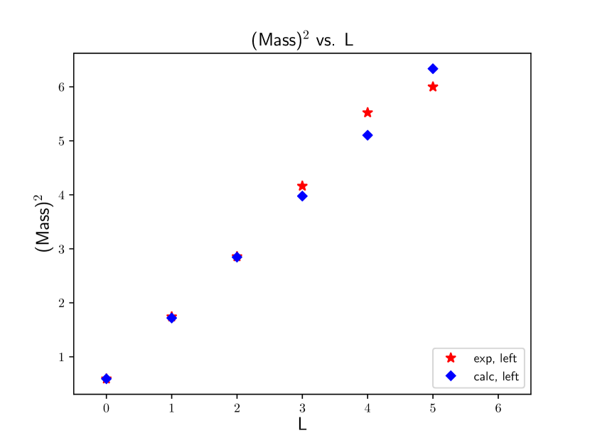
Figure 1: Regge slope

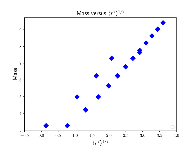
Figure 2: Mass versus r

Table 2: Meson mass versus RMS radius

$n$	$l$	$s$	mass(GeV)	radius(GeV)-1	$n$	$l$	$s$	mass(GeV)	radius(GeV)-1
0	0	0	0.140	3.261	2	0	0	1.629	6.245
0	0	1	0.770	3.261	2	0	1	2.259	6.245
0	1	0	1.311	4.210	2	1	0	2.496	6.789
0	1	1	1.311	4.210	2	1	1	2.496	6.789
0	2	0	1.687	4.982	2	2	0	2.713	7.293
0	2	1	1.687	4.982	2	2	1	2.713	7.293
0	3	0	1.994	5.649	2	3	0	2.913	7.764
0	3	1	1.994	5.649	2	3	1	2.913	7.764
0	4	0	2.259	6.245	2	4	0	3.101	8.208
0	4	1	2.259	6.245	2	4	1	3.101	8.208
0	5	0	2.496	6.789	2	5	0	3.277	8.629
0	5	1	2.496	6.789	2	5	1	3.277	8.629
1	0	0	1.057	4.982	3	0	0	2.083	7.293
1	0	1	1.687	4.982	3	0	1	2.713	7.293
1	1	0	1.994	5.649	3	1	0	2.913	7.640
1	1	1	1.994	5.649	3	1	1	2.913	7.764
1	2	0	2.259	6.245	3	2	0	3.101	8.208
1	2	1	2.259	6.245	3	2	1	3.101	8.208
1	3	0	2.496	6.789	3	3	0	3.277	8.629
1	3	1	2.496	6.789	3	3	1	3.277	8.629
1	4	0	2.713	7.293	3	4	0	3.445	9.031
1	4	1	2.713	7.293	3	4	1	3.445	9.031
1	5	0	2.913	7.764	3	5	0	3.605	9.415
1	5	1	2.913	7.764	3	5	1	3.605	9.415

V String Breaking

The second class of interactions allow the confined singlets to interact. The interaction is assumed to be a string-breaking interaction that assumes in the first approximation that a quark-anti-quark pair is produced with equal probability at any point on a line between the quark and anti-quark, causing it to break up into a pair of confined singlets. The interaction is taken to be local in the sense that the quark anti-quark pair is produced at a point. This is consistent with the assumption that string breaking is generated by the local covariant derivative operator. Since this naive interaction is singular, the delta functions that keep the produced pair on the line between the original quark and anti-quark are replaced by Gaussian approximations of delta functions where the width of the Gaussian is the same as the oscillator ground state. This has the effect of fattening the string to a flux tube with a width consistent with the size of the ground state. Given that QCD has only one coupling constant, it seems reasonable that the scale that determines the bare meson sizes should also determine the bare hadronic vertex form factors. Subsequent calculations using this vertex indicate that in order to get a consistent description of the Regge trajectories and the $\rho$ lifetime, it is necessary to use a unitary scale transformation to reduce the width of the flux tube by a factor of two (see equations (86-87). This transformation is applied after the vertex is computed. The resulting interaction is still consistent with the scale set by the confining interaction.

An additional virtue of this string breaking vertex is that it is possible to analytically perform the nine dimensional integrals that smear the vertex with one initial and two final confined quark anti-quark singlets. This property simplifies calculations with sea quarks.

The light-front translationally invariant, spin-independent part of the string-breaking vertex is taken to have a $r$-space kernel of the form

$$\langle\mathbf{r}_{1},\mathbf{r}_{2},\mathbf{r}_{12}|v_{2:1}|\mathbf{r}\rangle:=\gamma\delta(\mathbf{r}-2\mathbf{r}_{12})\int_{0}^{1}d\eta\delta_{\sqrt{{\lambda\over 2}}}(\mathbf{r}_{1}-\eta\mathbf{r})\delta_{\sqrt{{\lambda\over 2}}}(\mathbf{r}_{2}-(1-\eta)\mathbf{r})$$ (68)

where the Gaussian approximate delta function is

$$\delta_{\sqrt{{\lambda\over 2}}}(\mathbf{r}):=({\lambda\over 4\pi})^{3/2}e^{-\lambda r^{2}\over 4}\qquad\int\delta_{\sqrt{{\lambda\over 2}}}(\mathbf{r})d\mathbf{r}=1.$$ (69)

The coordinates are defined as Fourier transforms of the light-front invariant momentum variable $\mathbf{k}$. In order for matrix elements of this vertex to have dimensions of energy the matrix element

$$\langle\psi|v_{1:2}v_{2:1}|\psi\rangle\qquad v_{1:2}:=v_{2:1}^{\dagger}$$ (70)

should have dimension (energy)². It follows that $\gamma$ should have dimensions of (energy)^-1. Since $\lambda$ has dimension (energy)², it can be replaced by

$$\gamma\to g/\sqrt{\lambda}$$ (71)

which makes $g$ a dimensionless factor. Since the model assumption is that one parameter should fix all scales, the dimensionless parameter $g$ should be of order unity. In the calculations that follow $g$ was taken to be $5.44$. This choice gives a qualitatively consistent picture of the $\rho$ lifetime and the $\pi-\pi$ scattering cross section.

The variables $\mathbf{r}_{1}$ and $\mathbf{r}_{2}$ are the displacement variables of the quark-anti-quark pairs in the produced confined singlets. The variable $\mathbf{r}$ is the displacement variable for the quark-anti-quark pair in the initial confined singlet. The variable $\mathbf{r}_{12}$ represents the displacement between the centers of the two produced singlets. The assumption that the quark anti-quark pair is produced at a point leads to $\mathbf{r}=2\mathbf{r}_{12}$. The general structure is illustrated in figure 3.

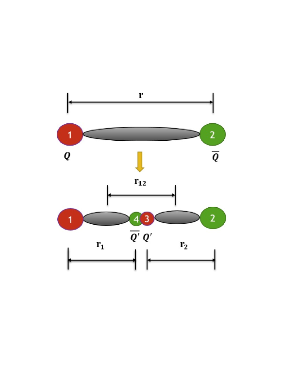
Figure 3: String breaking vertex

In the limit that the Gaussians become delta functions the interaction makes the string break with equal probability at any point along the line between the initial quark and anti-quark.

The hadronic vertices, which are defined by the overlap of this string-breaking vertex with three harmonic oscillator states can be computed analytically. The result, which is derived in appendix I and II is

$$\langle n_{1},l_{1},m_{1},n_{2},l_{2},m_{2},\mathbf{r}_{12}|v_{2:1}|n,l,m\rangle=$$

$$\int\psi_{n_{1}l_{1}m_{1}}^{*}(\mathbf{r}_{1})\psi_{n_{2}l_{2}m_{2}}^{*}(\mathbf{r}_{2})v(\mathbf{r}_{1},\mathbf{r}_{2},\mathbf{r}_{12};\mathbf{r})\psi_{nlm}(\mathbf{r})d\mathbf{r}_{1}d\mathbf{r}_{2}d\mathbf{r}=$$

$${g\over\sqrt{\lambda}}R_{nl}(2{r}_{12})({2\lambda})^{3/2}{(\sqrt{{\lambda\over 2}}{r}_{12})^{2n_{1}+l_{1}+2n_{2}+l_{2}}\over\sqrt{2n_{1}!\Gamma(n_{1}+l_{1}+{3\over 2}})\sqrt{2n_{2}!\Gamma(n_{2}+l_{2}+{3\over 2}})}\times$$

$$e^{-{\lambda\over 4}r_{12}^{2}}\sum_{k_{1}+k_{2}=2r}{(l_{1}+2n_{1})!(l_{2}+2n_{2})!\over k_{1}!k_{2}!(l_{1}+2n_{1}-k_{1})!(l_{2}+2n_{2}-k_{2})!}(-)^{k_{2}}({1\over 2})^{l_{1}+2n_{1}+l_{2}+2n_{2}}\times$$

$${1\over 2r+1}M({1\over 2}+r,{3\over 2}+r,-{\lambda r^{2}_{12}\over 4})Y_{lm}(\hat{\mathbf{r}}_{12})Y_{l_{1}m_{1}}^{*}(\hat{\mathbf{r}}_{12})Y_{l_{2}m_{2}}^{*}(\hat{\mathbf{r}}_{12}).$$ (72)

where $M({1\over 2}+r,{3\over 2}+r,-{\lambda r^{2}_{12}\over 4})$ is the confluent hypergeometric function.

This matrix element does not include any spin dependence. The model assumption is that the string breaking creates a quark anti-quark pair out of the vacuum at the point where the string breaks. In what follows the initial quark-anti-quark is labeled $1-2$, the pair created out of the vacuum is labeled $3-4$ and the final quark anti-quark pairs are labeled $1-4$ and $2-3$ (see figure 3). Since the quark and anti-quark have opposite parity, if they are created out of the vacuum the pair must be in an odd l state. Since the spin of the pair can be 0 or 1, to get $j=0$ and $l$ odd the quark and anti-quark must be created with $s=l=1$. The following spin-dependent addition is motivated by assuming that the string-breaking operator is oriented parallel to the original quark anti-quark pair

$$Y_{1m}(\hat{\mathbf{r}}_{12})\langle s_{3},\mu_{3},s_{4},\mu_{4}|1,\mu_{s}\rangle\langle 1,m_{l},1,\mu_{s}|0,0\rangle.$$ (73)

This operator is included as a dimensionless multiplicative factor. The directional dependence is motivated by the string breaking model, where the breaking is caused by a quark-anti-quark-link oriented parallel to the line between the quark and anti-quark. The $Y^{1}_{m_{1}}(\hat{\mathbf{r}}_{12})$ gives the spherical components of the unit vector along the line between original the quark and anti-quark. The full-spin dependence is obtained by multiplying this factor by an additional spin factor that couples the above to the spins of the other quarks and anti-quarks

$$\langle s_{23},\mu_{s23}|s_{2},\mu_{2},s_{3},\mu_{3}\rangle\langle s_{14},\mu_{s14}|s_{1},\mu_{1},s_{4},\mu_{4}\rangle\langle s_{1},\mu_{1},s_{2},\mu_{2}|s_{12},\mu_{s12}\rangle$$ (74)

and summing over the single quark spins.

The spin-dependent vertex is obtained by multiplying the spin-independent vertex by these two spin-dependent factors to get:

$$\langle n_{23},l_{23},m_{23},s_{23},\mu_{s23},n_{14},l_{14},m_{14},s_{14},\mu_{s14},\mathbf{r}_{12}|v_{2:1}|n_{12},l_{12},m_{12},s_{12},\mu_{s12}\rangle$$

$$\sum\langle n_{23},l_{23},m_{23},n_{14},l_{14},m_{14},\mathbf{r}_{12}|v_{2:1}|n_{12},l_{12},m_{12}\rangle Y_{1,m_{1}}(\hat{\mathbf{r}}_{12})\times$$

$$\langle{1\over 2},\mu_{3},{1\over 2},\mu_{4}|1,\mu_{s}\rangle\langle 1,m_{1},1,\mu_{s}|0,0\rangle\times$$

$$\langle s_{23},\mu_{s23}|s_{2},\mu_{2},s_{3},\mu_{3}\rangle\langle s_{14},\mu_{s14}|s_{1},\mu_{1},s_{4},\mu_{4}\rangle\langle s_{1},\mu_{1},s_{2},\mu_{2}|s_{12},\mu_{s12}\rangle.$$ (75)

The radial dependence can be projected on angular momentum states by multiplying by the spherical harmonic $\langle l_{v},m_{v}|\hat{\mathbf{r}}_{12}\rangle$ and integrating over angles. The resulting angular integral is over a product of five spherical harmonics

$$\langle 1_{14},m_{14}|\hat{\mathbf{r}}_{12}\rangle\langle 1_{23},m_{23}|\hat{\mathbf{r}}_{12}\rangle\langle l_{v},m_{v}|\hat{\mathbf{r}}_{12}\rangle\langle\hat{\mathbf{r}}_{12}|l_{12}m_{12}\rangle\langle\hat{\mathbf{r}}_{12}|1,m_{l34}\rangle=$$

$$Y^{*}_{l_{14}m_{14}}(\hat{\mathbf{r}}_{12})Y^{*}_{l_{23}m_{23}}(\hat{\mathbf{r}}_{12})Y^{*}_{l_{v}m_{v}}(\hat{\mathbf{r}}_{12})Y_{l_{12}m_{12}}(\hat{\mathbf{r}}_{12})Y_{1m_{1}}(\hat{\mathbf{r}}_{12}).$$ (76)

This integral can be expressed as sums of products of Clebsch-Gordan coefficients:

$$\int d\hat{\mathbf{r}}_{12}Y^{*}_{l_{14}m_{14}}(\hat{\mathbf{r}}_{12})Y^{*}_{l_{23}m_{23}}(\hat{\mathbf{r}}_{12})Y^{*}_{l_{v}m_{v}}(\hat{\mathbf{r}}_{12})Y_{l_{12}m_{12}}(\hat{\mathbf{r}}_{12})Y_{1m_{34}}(\hat{\mathbf{r}}_{12})=$$

$$\sum_{l_{t},l_{12:34}}\langle l_{14},m_{14},l_{23},m_{23}|l_{14:23},m_{l_{14:23}}\rangle\langle l_{14:23},m_{l_{14:23}},l_{v},m_{v}|l_{t},m_{t}\rangle\langle l_{t},m_{t}|l_{12},m_{12},1,m_{34}\rangle.$$ (77)

Since the bare meson states are eigenstates states of total angular momentum, it is useful to couple the spins and orbital angular momenta of each bare meson state. This involves multiplying by three more Clebsch-Gordan coefficients. The result for the vertex is

$$\langle n_{23},j_{23},l_{23},s_{23},\mu_{23},n_{14},j_{14},l_{14},s_{14},\mu_{14}{r},l_{v},m_{v}|v_{2:1}|n_{12},j_{12},l_{12},s_{12},\mu_{12}\rangle=$$

$$\langle n_{23},l_{23},n_{14},l_{14},{r}|v_{2:1}|n_{12},l_{12}\rangle\times C(j_{23},l_{23},s_{23},\mu_{23},j_{14},l_{14},s_{14},\mu_{14},l_{v},m_{v};j_{12},l_{12},s_{12},\mu_{12})$$ (78)

where

$$C(j_{23},l_{23},s_{23},\mu_{23},j_{14},l_{14},s_{14},\mu_{14},l_{v},m_{v};j_{12},l_{12},s_{12},\mu_{12}):=$$

$$\sum\langle j_{14},\mu_{14}|l_{14},m_{14},s_{14},\mu_{s14}\rangle\langle j_{23},\mu_{23}|l_{23},m_{23},s_{23},\mu_{s23}\rangle\times$$

$$\langle l_{14},m_{14},l_{23},m_{23}|l_{14:23},m_{l_{14:23}}\rangle\langle l_{14:23},m_{l_{14:23}},l_{v},m_{v}|l_{t},m_{t}\rangle\langle l_{t},m_{t}|l_{12},m_{12},1,m_{34}\rangle\times$$

$$\langle s_{23},\mu_{s23}|s_{2},\mu_{2},s_{3},\mu_{3}\rangle\langle s_{14},\mu_{s14}|s_{1},\mu_{1},s_{4},\mu_{4}\rangle\langle s_{1},\mu_{1},s_{2},\mu_{2}|s_{12},\mu_{s12}\rangle\times$$

$$\langle s_{3},\mu_{3},s_{4},\mu_{4}|1,\mu_{s}\rangle\langle 1,m_{l},1,\mu_{s}|0,0\rangle\langle l_{12},m_{12},s_{12},\nu_{s12}|j_{12},\nu_{12}\rangle.$$ (79)

This has the form of the product of the spin-independent vertex (199) multiplied by a spin-dependent coefficient (79).

The more useful form is the momentum-space version of these vertices. They can be obtained by performing a Fourier-Bessel transform of the vertex (78). Because the spin-independent vertex factors out of this expression it is enough to replace the spin-independent coefficient

$$\langle n_{23},l_{23},n_{14},l_{14},{r}|v_{2:1}|n_{12},l_{12}\rangle$$ (80)

in the above expression by its Fourier-Bessel transform

$$\langle n_{23},l_{23},n_{14},l_{14},{\kappa},l_{v}|v_{2:1}|n_{12},l_{12}\rangle:=\sqrt{{2\over\pi}}\int_{0}^{\infty}r^{2}drj_{l_{v}}(\kappa r)\langle n_{23},l_{23},n_{14},l_{14},{r}|v_{2:1}|n_{12},l_{12}\rangle$$ (81)

so the momentum-space vertex becomes

$$\langle n_{23},j_{23},l_{23},s_{23},\mu_{23},n_{14},j_{14},l_{14},s_{14},\mu_{14},\kappa,l_{v},m_{v}|v_{2:1}|n_{12},j_{12},l_{12},s_{12},\mu_{12}\rangle=$$

$$\langle n_{23},l_{23},n_{14},l_{14},\kappa,l_{v}|v_{2:1}|n_{12},l_{12}\rangle\times C(j_{23},l_{23},s_{23},\mu_{23},j_{14},l_{14},s_{14},\mu_{14},l_{v},m_{v};j_{12},l_{12},s_{12},\mu_{12}).$$ (82)

Both the strength and size scale of the vertex is determined by the same parameter that is responsible for the confinement. This elementary string breaking vertex at the quark level leads to analytic expressions for all vertices relating one bare confined meson eigenstate to two bare confined meson eigenstates as a function of the initial relative quark-anti-quark displacement.

The only integral that needs to be computed numerically is the one-dimensional radial integral in the Fourier-Bessel transform. While the model is too crude to expect that all of these vertices lead to accurate results, the hope is that they provide a rough characterization of the size of the contributions from the higher lying states assuming that the physics is largely determined by the string-breaking mechanism.

This vertex has the property that the kernel of this operator is rotationally covariant:

$$\sum D^{j_{23}}_{\mu_{23}\nu_{23}}[R]D^{j_{14}}_{\mu_{14}\nu_{14}}[R]D^{l_{v}}_{m_{v}m_{v}^{\prime}}[R]\langle n_{23},j_{23},l_{23},s_{23},\nu_{23},n_{14},j_{14},l_{14},s_{14},\nu_{14}\kappa,l_{v},m_{v}^{\prime}|v_{2:1}|n_{12},j_{12},l_{12},s_{12},\mu_{12}\rangle=$$

$$\sum\langle n_{23},j_{23},l_{23},s_{23},\mu_{23},n_{14},j_{14},l_{14},s_{14},\mu_{14},\kappa,l_{v},m_{v}|v_{2:1}|n_{12},j_{12},l_{12},s_{12},\nu_{12}\rangle D^{j_{12}}_{\nu_{12}\mu_{12}}[R].$$ (83)

This is also true for the $r$-space vertex. This means that the operator is rotationally invariant. This property will be important in making a Poincaré invariant dynamics that includes the vertex. This will be discussed in the next section.

For the purpose of using this vertex in a relativistic light-front dynamical model it is useful decompose this vertex into invariant kernels for different partial waves. This is achieved by coupling the final meson spins and relative orbital angular momenta

$$\langle(\kappa,j)n_{23},j_{23},l_{23},s_{23},n_{14},j_{14},l_{14},s_{14},l_{v},s,\tilde{\mu}|v^{j}_{2:1}|n_{12},j_{12},l_{12},s_{12},\tilde{\mu}^{\prime}\rangle=$$

$$\delta_{jj_{12}}\delta_{\tilde{\mu}\tilde{\mu}^{\prime}}\langle n_{23},l_{23},n_{14},l_{14},\kappa,l_{v}|v_{2:1}|n_{12},l_{12}\rangle\times G^{j}(j_{23},l_{23},s_{23},j_{14},l_{14},s_{14},l_{v},s;l_{12},s_{12})$$ (84)

where the rotationally invariant coefficient can be computed by using rotational covariance and integrating over the $SU(2)$ Haar measure, which is equivalent to averaging over the magnetic quantum numbers

$$G^{j}(j_{23},l_{23},s_{23},j_{14},l_{14},s_{14},l_{v},s;l_{12},s_{12}):=$$

$${1\over 2j+1}\sum_{\mu_{12}=-j}^{j}C(j_{23},l_{23},s_{23},\mu_{23},j_{14},l_{14},s_{14},\mu_{14},l_{v},m_{v};j,l_{12},s_{12},\mu_{12})\langle j,\mu_{12}|l_{v},m_{v},s,\mu_{s}\rangle\langle s,\mu_{s}|j_{23},\mu_{23},j_{14},\mu_{14}\rangle.$$ (85)

The spins in (84) are the system light-front spins.

Qualitative agreement with the $\rho$ lifetime was used to determine the dimensionless strength, $g$ of the string breaking interaction. In order to achieve the desired agreement, in addition to using the freedom to make order of unity adjustments to the strength, it was also necessary to make the following scale transformation on the vertex on the spin-independent part of the string breaking vertex

$$\langle n_{23},l_{23},n_{14},l_{14},r|v_{2:1}|n_{12},l_{12}\rangle\to\langle n_{23},l_{23},n_{14},l_{14},r|v^{\prime}_{2:1}|n_{12},l_{12}\rangle:=$$

$$(2)^{3/2}\langle n_{23},l_{23},n_{14},l_{14},2r|v_{2:1}|n_{12},l_{12}\rangle$$ (86)

and

$$\langle n_{23},l_{23},n_{14},l_{14},\kappa,l_{v}|v_{2:1}|n_{12},l_{12}\rangle\to\langle n_{23},l_{23},n_{14},l_{14},\kappa,l_{v}|v^{\prime}_{2:1}|n_{12},l_{12}\rangle:=$$

$$(2)^{-3/2}\langle n_{23},l_{23},n_{14},l_{14},{\kappa\over 2},l_{v}|v_{2:1}|n_{12},l_{12}\rangle.$$ (87)

This scale transformation has the effect of reducing the width of the string breaking vertex by a factor of two, which is still a modification of order unity of the original string breaking vertex. The calculations that follow use the re-scaled vertex unless otherwise specified.

Figure 4 shows the strength of the spin-independent part (80) of the re-scaled vertices for $l_{23}=l_{14}=l_{12}=0$ and different values of $n_{23}=n_{14}=n_{12}=n$. The lower $n$ contributions dominate at lower energies. The contribution for each $n$ is significant in a given energy range and falls off rapidly outside of that range. We note that most of the computational complexity is due to the spin coupling.

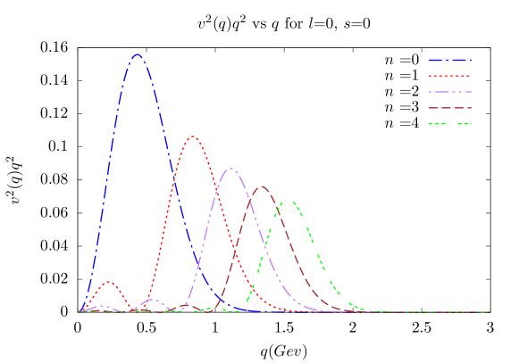
Figure 4: Strength of vertex as value of n changes for l=0 s=0

VI Sea Quarks - Relativistic 1$+$2 Model

The simplest extension of the bare confined singlet model allows the bare confined singlets to interact with the string breaking vertex to produce pairs of bare confined singlets. The model Hilbert space is the orthogonal direct sum of the one-singlet Hilbert space with the tensor product of two copies of the one-singlet Hilbert space

$${\cal H}={\cal H}_{H}\oplus({\cal H}_{H}\otimes{\cal H}_{H}).$$ (88)

This is unitarily equivalent to the corresponding representation in terms of confined quark-anti-quark-gluon singlet pairs

$${\cal H}={\cal H}_{Q}\oplus({\cal H}_{Q}\otimes{\cal H}_{Q}).$$ (89)

This equivalence exhibits the duality between representations in terms of one and two quark-anti-quark-gluon singlet pairs and one in terms of infinite towers of one or two bare mesons. In this case the two-singlet or two-bare meson sectors represent sea quark degrees of freedom.

In section 3 a unitary representation of the Poincaré group on the single-meson states (55), was constructed in both the hadronic (58) and quark (60) representations

$$U(\Lambda,a):{\cal H}_{H}\to{\cal H}_{H}$$ (90)

$$U(\Lambda,a):{\cal H}_{Q}\to{\cal H}_{Q}.$$ (91)

The next step is to construct a relativistic dynamics on the Hilbert space (88-89). The first step is to use (90-91) to define the free dynamics on the space (88)

$$U_{0}(\Lambda,a)=\left(\begin{array}[]{cc}U(\Lambda,a)&0\\ 0&U(\Lambda,a)\otimes U(\Lambda,a)\\ \end{array}\right).$$ (92)

Here free means free bare mesons, not free quarks. This representation treats the bare mesons as if they were elementary particles. This representation has to be modified to include the dynamics defined by the string-breaking vertex.

The next step in constructing a relativistic dynamics is to decompose the operator $U_{0}(\Lambda,a)$ into a direct integral of irreducible representations. This can be done by decomposing the direct product of single-particle irreducible basis states into a direct integral of irreducible basis states using the Poincaré group Clebsch-Gordan coefficients in the light front basis: (34)

$$|(\kappa,j)\tilde{\mathbf{p}},\tilde{\mu};n_{1},j_{1},l_{1},s_{1},n_{2},l_{2},s_{2},s_{12},l_{12}\rangle=$$

$$\sum|(M_{n_{1},l_{1},s_{1}},j_{1})\tilde{\mathbf{p}}_{1},\mu_{1}\rangle|(M_{n_{2},l_{2},s_{2}},j_{2})\tilde{\mathbf{p}}_{2},\mu_{2}\rangle D^{j_{1}}_{\mu_{1},\nu_{1}}[R_{fc}(k_{1}/M_{n_{1},j_{1},l_{1},s_{1}})]D^{j_{2}}_{\mu_{2},\nu_{2}}[R_{fc}(k_{2}/M_{n_{2},j_{2},l_{2},s_{2}})]\times$$

$$Y_{l_{12}m_{12}}(\hat{\mathbf{q}}_{1})\langle j_{1},\nu_{1},j_{2},\nu_{2}|s_{12}\nu_{12}\rangle\langle l_{12},m_{12},s_{12},\nu_{12}|j,\tilde{\nu}\rangle\sqrt{{p_{1}^{+}p_{2}^{+}(\omega_{1}(\kappa)+\omega_{2}(\kappa))\over\omega_{1}(\kappa)\omega_{2}(\kappa)(p_{1}^{+}+p_{2}^{+})}}$$ (93)

where in this representation the two-body kinematic mass is the multiplication operator

$$M_{02}:=\omega_{1}(\kappa)+\omega_{2}(\kappa)=\sqrt{\kappa^{2}+M_{n_{1},j_{1},l_{1},s_{1}}^{2}}+\sqrt{\kappa^{2}+M_{n_{2},j_{2},l_{2},s_{2}}^{2}}.$$ (94)

The states

$$\left(\begin{array}[]{c}|(M_{nls},j)\tilde{\mathbf{p}},\tilde{\mu};l,s\rangle\\ 0\\ \end{array}\right)$$ (95)

and

$$\left(\begin{array}[]{c}0\\ |(\kappa,j)\tilde{\mathbf{p}},\tilde{\mu};n_{1},j_{1},l_{1},s_{1},n_{2},l_{2},s_{2},s_{12},l_{12}\rangle\end{array}\right).$$ (96)

are a basis that transforms irreducibly under $U_{0}(\Lambda,a)$:

$$U_{0}(\Lambda,a)\left(\begin{array}[]{c}|(M_{nls},j)\tilde{\mathbf{p}},\tilde{\mu};l,s\rangle\\ 0\\ \end{array}\right)=$$

$$\left(\begin{array}[]{c}|(M_{nls},j)\tilde{\boldsymbol{\Lambda}}p,\tilde{\nu};l,s\rangle\\ 0\\ \end{array}\right)e^{-i\Lambda p\cdot a}D^{j}_{\tilde{\nu}\tilde{\mu}}[B_{f}^{-1}(\Lambda p/M_{nls})\Lambda B_{f}(p/M_{nls})]\sqrt{{(\Lambda p)^{+}\over p^{+}}}.$$ (97)

$$U_{0}(\Lambda,a)\left(\begin{array}[]{c}0\\ |(\kappa,j)\tilde{\mathbf{p}},\tilde{\mu};n_{1},j_{1},l_{1},s_{1},n_{2},l_{2},s_{2},s_{12},l_{12}\rangle\end{array}\right)=$$

$$\left(\begin{array}[]{c}0\\ |(\kappa,j)\tilde{\boldsymbol{\Lambda}}p,\tilde{\nu};n_{1},j_{1},l_{1},s_{1},n_{2},l_{2},s_{2},s_{12},l_{12}\rangle\end{array}\right)e^{-i\Lambda p\cdot a}D^{j}_{\tilde{\nu}\tilde{\mu}}[B_{f}^{-1}(\Lambda p/M_{02})\Lambda B_{f}(p/M_{02})]\sqrt{{(\Lambda p)^{+}\over p^{+}}}.$$ (98)

The next step is to express the kernel of the vertex operator in this basis:

$$\langle(\kappa,j)\tilde{\mathbf{p}},\tilde{\mu};n_{1},j_{1},l_{1},s_{1},n_{2},l_{2},s_{2},s_{12},l_{12}|v_{2:1}|(n,j^{\prime})\tilde{\mathbf{p}}^{\prime},\tilde{\mu}^{\prime};l,s\rangle=$$

$$\delta_{jj^{\prime}}\delta_{\tilde{\mu}\tilde{\mu}^{\prime}}\delta(\tilde{\mathbf{p}}-\tilde{\mathbf{p}}^{\prime})\langle n_{1},l_{1},n_{2},l_{2},\kappa,l_{12}|v_{2:1}|n,l\rangle\times G^{j}(j_{1},l_{1},s_{1},j_{2},l_{2},s_{2},l_{12},s_{12};l,s)$$ (99)

where $G^{j}(j_{1},l_{1},s_{1},j_{2},l_{2},s_{2},l_{12},s_{12};l,s)$ is the spin coefficient in (85). Using this vertex the dynamical mass operator is defined by

$$M=M_{0}+V=\underbrace{\left(\begin{array}[]{cc}M_{c}&0\\ 0&\sqrt{M_{c1}^{2}+{\kappa}^{2}}+\sqrt{M_{c2}^{2}+{\kappa}^{2}}\\ \end{array}\right)}_{M_{0}}+\underbrace{\left(\begin{array}[]{cc}0&v_{1:2}\\ v_{2:1}&0\\ \end{array}\right)}_{V},$$ (100)

where $M_{0}$ is the mass Casimir operator of $U_{0}(\Lambda,a)$. With this definition $M$ commutes with $\tilde{\mathbf{p}}$ and $\mathbf{j}$ but not with $M_{0}$ because $[M_{0},V]\not=0$. This means that it is possible to simultaneously diagonalize $M$, $\tilde{\mathbf{p}}$, $j^{2}$ and $j_{z}$. If this is done in the basis of simultaneous eigenstates of $M_{0}$, $\tilde{\mathbf{p}}$, $j^{2}$ and $j_{z}$ then it is only necessary to diagonalize $M$. The resulting eigenfunctions have the form

$$\langle j,\tilde{p},\tilde{\mu},\cdots|(m,j^{\prime})\tilde{p}^{\prime},\tilde{\mu}^{\prime};X\rangle=\left(\begin{array}[]{c}\langle(M_{nls},j)\tilde{\mathbf{p}},\tilde{\mu};l,s|(m,j^{\prime})\tilde{\mathbf{p}}^{\prime},\tilde{\mu}^{\prime};X\rangle\\ \langle(\kappa,j)\tilde{\mathbf{p}},\tilde{\mu};n_{1},j_{1},l_{1},s_{1},n_{2},l_{2},s_{2},s_{12},l_{12}|(m,j^{\prime})\tilde{\mathbf{p}}^{\prime},\tilde{\mu}^{\prime};X\rangle\\ \end{array}\right)=$$

$$\delta(\tilde{\mathbf{p}}^{\prime}-\tilde{\mathbf{p}})\delta_{j^{\prime}j}\delta_{\tilde{\mu}^{\prime}\tilde{\mu}}\times\left(\begin{array}[]{c}\langle(M_{nls},j)l,s|(m,j);X\rangle\\ \langle(\kappa,j);n_{1},j_{1},l_{1},s_{1},n_{2},l_{2},s_{2},s_{12},l_{12}|(m,j);X\rangle\\ \end{array}\right)$$ (101)

where $X$ represents possible degeneracy parameters.

The rotational invariance of (100) means that the rest eigenstates in this representation transform under the $2j+1$ dimensional representation of the $SU(2)$.

A dynamical unitary representation of the Poincaré group with a light-front kinematic symmetry is defined in this basis by

$$U(\Lambda,a)|(m,j)\tilde{\mathbf{p}},\tilde{\mu},X\rangle:=|(m,j)\tilde{\boldsymbol{\Lambda}}p,\tilde{\nu},X\rangle e^{-i\Lambda p\cdot a}D^{j}_{\tilde{\nu}\tilde{\mu}}[B_{f}^{-1}(\Lambda p/m)\Lambda B_{f}(p/m)]\sqrt{{(\Lambda p)^{+}\over p^{+}}}.$$ (102)

This reduces the dynamical problem to finding the eigenvalues of the mass operator in the kinematic irreducible basis. The representation (102) has the property that $e^{i\Lambda p\cdot a}$, $D^{j}_{\nu\mu}[B_{f}^{-1}(\Lambda p/m)\Lambda B_{f}(p/m)]$ and $\sqrt{{(\Lambda p)^{+}\over p^{+}}}$ are all independent of $m$ for all Poincaré transformations that leave the light front invariant. Since the interaction only changes the mass in this representation, it follows that the light-front-preserving subgroup is kinematic. This means that for these light-front-preserving Lorentz transformations

$$\left(\begin{array}[]{c}\langle(M_{nls},j)\tilde{\mathbf{p}},\tilde{\mu};l,s|U(\Lambda,a)|(m,j^{\prime})\tilde{p}^{\prime},\tilde{\mu}^{\prime};X\rangle\\ \langle(\kappa,j)\tilde{\mathbf{p}},\tilde{\mu};n_{1},j_{1},l_{1},s_{1},n_{2},l_{2},s_{2},s_{12},l_{12}|U(\Lambda,a)|(m,j^{\prime})\tilde{p}^{\prime},\tilde{\mu}^{\prime};X\rangle\\ \end{array}\right),$$ (103)

can be evaluated by acting to the right on the irreducible eigenstate or to the left with the adjoint on the non-interacting basis state.

Equation (102) defines $U(\Lambda,a)$ on a complete set of irreducible states. This defines a relativistic light-front dynamics on this space that is consistent with the dynamical mass operator. This model has the advantage that the mass operator is exactly rotationally invariant. Given these eigenstates they can be transformed to single-quark bases or any other convenient basis.

In what follows calculations will used to investigate to what extent this simple model provides a qualitatively consistent description of the following observables:

• Probability of finding sea quarks in bound states.

• Cross section for scattering of bare mesons.

• Lifetimes and energy shifts of unstable bare mesons.

• Convergence as the number of bare meson channels are increased.

• Form factor calculations.

VII Bound States

The first question of interest is how do the sea quark contributions generated by the string-breaking vertex impact the mass spectrum and the sea quark content of the mesons. Clearly the eigenvalues of the lowest-mass bare mesons will shift and it will make the high-lying bare mesons unstable.

In the hadronic representation the bound state problem requires solving a system of equations with an infinite number of coupled channels.

Bound-states are eignevectors of $M=(M_{0}+V)$ with eigenvalues $\eta$ in the point spectrum:

$$(M_{0}+V)|\Psi\rangle=\eta|\Psi\rangle.$$ (104)

Truncating to the one $+$ two-bare meson sectors the mass eigenvalue equation has the operator form

$$\left(\begin{array}[]{cc}M_{c}&v_{1:2}\\ v_{2:1}&\sqrt{M_{c1}^{2}+{\kappa}^{2}}+\sqrt{M_{c2}^{2}+{\kappa}^{2}}\end{array}\right)\left(\begin{array}[]{c}|\psi_{1}\rangle\\ |\psi_{2}\rangle\end{array}\right)=\eta\left(\begin{array}[]{c}|\psi_{1}\rangle\\ |\psi_{2}\rangle\end{array}\right)$$ (105)

where $M_{c}$ is the bare quark-anti-quark mass operator, (47). These equations are equivalent to the pair of coupled equations

$$|\Psi_{1}\rangle={1\over\eta-M_{c}}v_{1:2}|\Psi_{2}\rangle$$ (106)

$$|\Psi_{2}\rangle={1\over\eta-\sqrt{M_{c1}^{2}+{\kappa}^{2}}-\sqrt{M_{c2}^{2}+{\kappa}^{2}}}v_{2:1}|\Psi_{1}\rangle.$$ (107)

Using the second equation in the first gives a single equation for the valence component, $|\Psi_{1}\rangle$:

$$\left(I-{1\over\eta-M_{c}}v_{1:2}{1\over\eta-\sqrt{M_{c1}^{2}+\kappa^{2}}+\sqrt{M_{c2}^{2}+\kappa^{2}}}v_{2:1}\right)|\Psi_{1}\rangle=0.$$ (108)

The exact meson mass eigenvalues are the real values of $\eta$ between zero and the two-bare meson threshold, where (108) has non-zero solutions.

The short-hand notation is used

$$m\leftrightarrow\{n_{1},j_{1},l_{1},s_{1}\}$$ (109)

$$n_{1},n_{2},\kappa\leftrightarrow\{s_{12},l_{q},n_{1},j_{1},l_{1},s_{1},n_{2},j_{2},l_{2},s_{2}\}$$ (110)

to label the one and two singlet channels, and

$$M_{n}:=M_{nls}\qquad M_{n_{1},n_{2}}(\kappa):=\sqrt{\kappa^{2}+M^{2}_{n_{1},l_{1},s_{1}}}+\sqrt{\kappa^{2}+M^{2}_{n_{2},l_{2},s_{2}}}$$ (111)

to label the mass eigenvalues of the bare meson systems. In this notation the mass eigenvalue problem (108) has the form

$$\sum_{m}\left(\delta_{nm}-\sum_{n_{1},n_{2}}\int_{0}^{\infty}{1\over\eta-M_{n}}\langle n|v_{1:2}|n_{1},n_{2},\kappa\rangle{\kappa^{2}d\kappa\over\eta-M_{n_{1},n_{2}}(\kappa)}\langle n_{1},n_{2},\kappa|v_{2:1}|m\rangle\right)\langle m|\Psi_{1}\rangle=0.$$ (112)

Even this truncated problem is a coupled channel problem with an infinite number of channels. It can be solved by an additional truncation to a finite number of channels. The ability to analytically calculate vertices that couple any combination of channels can be used to estimate the size of the error due to eliminated channels.

Equation (112) has the form

$$\sum_{m}(\delta_{nm}-A(\eta)_{nm})\langle m|\Psi_{1}\rangle=0.$$ (113)

The eigenvalues are the real zeros, $\eta_{k}$, of the determinant of the matrix, $\delta_{nm}-A(\eta)_{nm}$, considered a function of $\eta$:

$$f(\eta)=\mbox{det}(I-A(\eta))=0.$$ (114)

The eigenvalues, which are the zeroes of the determinant, can be determined by plotting the determinant, $f(\eta)$, for values of $\eta$ between 0 and the two meson threshold. For this range of values of $\eta$, the determinant is a real valued function of $\eta$ and the momentum integrals in (112) are non-singular.

To determine the wave function for the $k^{th}$ eigenvalue, $\eta_{k}$, consider the ordinary eigenvalue problem for $\chi$:

$$\sum_{m}(\chi\delta_{nm}-A_{nm}(\eta_{k}))\xi_{m}^{k}=0$$ (115)

By construction $\chi=1$ is the eigenvalue of this equation for $\eta=\eta_{k}$. The valence wave function in the hadronic representation is

$$\langle n|\Psi_{1}\rangle=N_{k}\xi^{k}_{n}$$ (116)

where $\xi^{1}_{n}$ is the eigenvector associated with $\chi=1$ of (115) and $N_{k}$ is a normalization constant.

The sea quark component of the wave function is

$$\langle n_{1},n_{2},\kappa|\Psi_{2}\rangle=\sum_{m}{1\over\eta_{k}-M_{n_{1},n_{2}}(\kappa)}\langle n_{1},n_{2},\kappa|v_{2:1}|m\rangle{1\over\eta_{k}-M_{m}}N_{k}\xi^{k}_{m}.$$ (117)

The normalization constant $N_{k}$ is chosen so

$$1=\langle\Psi_{1}|\Psi_{1}\rangle+\langle\Psi_{2}|\Psi_{2}\rangle.$$ (118)

With this normalization $\langle\Psi_{1}|\Psi_{1}\rangle$ represents the probability of finding the meson in the valence sector and $\langle\Psi_{2}|\Psi_{2}\rangle$ represents the probability of finding the meson with sea quarks.

The evaluation of $\langle\Psi_{2}|\Psi_{2}\rangle$ involves a one-dimensional integral and a sum over two hadron states that couple to the valence sector.

These “exact calculations” can be compared to the perturbative result to determine the applicability of perturbation theory. The perturbative calculation treats the string breaking interaction as a perturbation. A formal expansion parameter $\epsilon$ is introduced to keep track of powers of the string breaking vertex. In the end it is set to 1. The unperturbed state is taken to be one of the low-mass confined quark-anti-quark states ($n_{0}=m_{0},l_{0}$):

$$\left(\begin{array}[]{c}|\Psi_{10}\rangle\\ |\Psi_{20}\rangle\end{array}\right)=\left(\begin{array}[]{c}\delta_{nn_{0}}\\ 0\end{array}\right).$$ (119)

Standard Rayleigh-Schrödinger perturbation theory gives the leading correction to the unperturbed eigenvalue $M_{n_{0}}$ in powers of $\epsilon$:

$$M_{n_{0}}(\epsilon)=M_{n_{0}}+\epsilon^{2}\sum_{n_{1}n_{2}}\int\kappa^{2}d\kappa{|\langle n_{0}|v_{12}|n_{1},n_{2},\kappa\rangle|^{2}\over M_{n_{0}}-M_{n_{1},n_{2}}(\kappa)}+o(\epsilon^{4}).$$ (120)

The corresponding un-normalized wave function is

$$\left(\begin{array}[]{c}\langle n|\Psi_{1}\rangle\\ \langle n_{1},n_{2},\kappa|\Psi_{2}\rangle\end{array}\right)=\left(\begin{array}[]{c}\delta_{nn_{0}}\\ \epsilon{\langle n_{1},n_{2},\kappa|v_{21}|n_{0}\rangle\over M_{n_{0}}-M_{n_{1},n_{2}}(\kappa)}\end{array}\right)+\cdots$$ (121)

In what follows the model calculation uses a bare $\pi$ mass of $m_{\pi 0}=.16$ GeV, a bare $\rho$ mass of $m_{\rho 0}=.882$ GeV and a dimensionless vertex coupling constant $g=5.44$. The correction to the pion mass and wave function, keeping the 2 quark-2 anti-quark channels with $n\leq 4$, is computed using both second order perturbation theory (120) and the exact calculation obtained by finding zeroes of the determinant (114). The perturbative result gives a pion mass of $.1327$ GeV while the exact method gives a pion mass of $.1329$ GeV. While the perturbative and “exact” calculated masses are close, they differ from the bare $\pi$ mass of $.16$ GeV by about $.027$ GeV, which is about a 17% shift. The calculation of the corresponding pion wave function results in a probability of .82 of measuring the pion to be in the valence sector and .18 of measuring pion to be in a two bare singlet state. This indicates that in this model sea quarks make up a non-trivial part of the pion wave function.

VIII Meson-Meson Scattering

This model can also be used to treat meson-meson scattering. Due to the truncation, the particles that scatter are bare mesons. The scattering integral equations have an infinite number of poles in the continuum. These are not real, because the vertex makes the associated mesons unstable. The treatment of scattering in models with confined particles is discussed in R. F. Dashen et al. (1976)Dashen et al. (1976). These results are applicable to this model.

In this dual quark-hadron setting it is natural to formulate the scattering problem using a two Hilbert space formulation Coester and Polyzou (1982). In one Hilbert space, the asymptotic space, the bare mesons are treated like elementary particles. Their internal structure is included in a mapping from the asymptotic space to the dynamical Hilbert space. The asymptotic Hilbert space is the direct sum of scattering channel Hilbert spaces. The $2+1$ model scattering channels involve pairs of bare mesons labeled by the quantum numbers $n_{1}$ and $n_{2}$. A normalizable vector in the two bare-meson subspace of the Hilbert space has the form

$$|\Psi_{0n_{1}n_{2}}(0)\rangle=\sum_{\tilde{\mu}_{1}\tilde{\mu}_{2}}\int d\tilde{p}_{1},d\tilde{p}_{2}|(n_{1})\tilde{p}_{1},\tilde{\mu}_{1}\rangle\times|(n_{2})\tilde{p}_{2},\tilde{\mu}_{2}\rangle f_{n_{1}}(\tilde{p}_{1},\tilde{\mu}_{1})f_{n_{2}}(\tilde{p}_{2},\tilde{\mu}_{2})$$ (122)

where $f_{n_{1}}(\tilde{p}_{1},\tilde{\mu}_{1})$ and $f_{n_{2}}(\tilde{p}_{2},\tilde{\mu}_{2})$ are wave packets in the meson momenta and magnetic quantum numbers and the $n_{i}$ represent the particle quantum numbers $(n_{i},j_{i},l_{i},s_{i})$. Equation (122) can be expressed in the form of a mapping from the Hilbert space ${\cal H}_{n_{1}n_{2}}$ of square integrable functions of light-front momenta and meson magnetic quantum numbers to the two bare-mesons subspace of the Hilbert space:

$$|\Psi_{0n_{1}n_{2}}(0)\rangle:=\Phi_{0n_{1}n_{2}}|f_{n_{1}}f_{n_{2}}\rangle.$$ (123)

For identical mesons this state should be symmetrized:

$$|\Psi_{0n_{1}n_{2}}\rangle\to|\Psi_{0,{\cal S},n_{1},n_{1}}\rangle={\cal S}|\Psi\rangle$$ (124)

where ${\cal S}$ is the projector on symmetrized states. Note that in this model the symmetrization is only with respect to identical mesons, not quarks. The symmetrizer and normalization factors can be absorbed in the definition of $\Phi_{0n_{1}n_{2}}$, In both cases the free two-meson states should be normalized to unity:

$$\||\Psi_{0n_{1}n_{2}}(0)\rangle\|=1.$$ (125)

The asymptotic Hilbert space is defined as the orthogonal direct sum of all of the channel spaces:

$${\cal H}_{A}:=\oplus_{n_{1},n_{2}}{\cal H}_{n_{1},n_{2}}.$$ (126)

In this model there are an infinite number of channel subspaces. This is an artifact of the truncation to the $2+1$ sector, which eliminates the interactions in the two-meson subspace that allow unstable bare mesons to decay.

An injection operator from ${\cal H}_{A}$ to the two-meson subspace of the $2+1$ Hilbert space ${\cal H}$ is defined by

$$\Phi:=\sum_{n_{1},n_{2}}\Phi_{0n_{1}n_{2}}$$ (127)

where each $\Phi_{0n_{1}n_{2}}$ is understood to act on the subspace ${\cal H}_{n_{1},n_{2}}$ of ${\cal H}_{A}$. The two Hilbert space representation separates the quantities (momenta and magnetic quantum numbers) that are used to prepare initial and final meson wave packets from the internal structure of each meson in terms of quarks, anti-quarks and gluons. The asymptotic space contains the degrees of freedom that can be “controlled in an experiment”.

A light-front asymptotic Hamiltonian and mass operator is defined on ${\cal H}_{A}$. On each subspace ${\cal H}_{n_{1},n_{2}}$ they are:

$$P^{-}_{A}={M_{cn1}^{2}+\mathbf{p}_{n_{1}\perp}^{2}\over p_{n_{1}}^{+}}+{M_{cn2}^{2}+\mathbf{p}_{n_{2}\perp}^{2}\over p_{n_{2}}^{+}}$$ (128)

and

$$M_{A}=\sqrt{M_{cn1}^{2}+\kappa^{2}}+\sqrt{M_{cn2}^{2}+\kappa^{2}}.$$ (129)

In the absence of the string breaking vertex the asymptotic states evolve in time like two free particles (mesons)

$$|\Psi_{0n_{1}n_{2}}(t)\rangle=\Phi_{0n_{1}n_{2}}e^{-{i\over 2}(P_{A}^{-}+P_{A}^{+})t}|f_{n_{1}}f_{n_{2}}\rangle$$ (130)

Dynamical solutions of the Schrödinger equation $|\Psi_{\pm n_{1}n_{2}}(t)\rangle$ that look like these states long before or long after interacting satisfy the scattering asymptotic conditions

$$\lim_{t\to\pm\infty}\||\Psi_{\pm n_{1}n_{2}}(t)\rangle-|\Psi_{\pm 0n_{1}n_{2}}(t)\rangle\|=0$$ (131)

where $|\Psi_{\pm 0n_{1}n_{2}}(t)\rangle$ are free meson states of the form (130) that are approached by the exact scattering states in the asymptotic future $(+)$ or past $(-)$.

Using the unitarity of the time evolution operator this can be expressed as

$$\lim_{t\to\pm\infty}\||\Psi_{\pm n_{1}n_{2}}(0)\rangle-e^{i{1\over 2}(P^{-}+P^{+})t}\Phi_{n_{1}n_{2}}e^{-{i\over 2}(P_{A}^{-}+P_{A}^{+})t}|f_{n_{1}}f_{n_{2}}\rangle\|=0.$$ (132)

Since $P^{+}$ and $\mathbf{P}_{\perp}$ are kinematic operators (132) becomes

$$\lim_{t\to\pm\infty}\||\Psi_{\pm}(0)\rangle-e^{i{M^{2}\over 2P^{+}}t}\Phi_{0n_{1}n_{2}}e^{-i{M_{A}^{2}\over 2P^{+}}t}|f_{n_{1}}f_{n_{2}}\rangle\|=0.$$ (133)

Because the spectrum of $P^{+}$ is positive, the time limit can be replaced by a $\tau:={t/2P^{+}}$ limit:

$$\lim_{\tau\to\pm\infty}\||\Psi_{\pm n_{1}n_{2}}(0)\rangle-e^{iM^{2}\tau}\Phi_{0n_{1}n_{2}}e^{-iM_{A}^{2}\tau}|f_{n_{1}}f_{n_{2}}\rangle\|=0.$$ (134)

Finally the invariance principle Reed and Simon (1979)Chandler and Gibson (1976) can be used to replace $M^{2}$ by $M$ leading to the following expression for the normalized scattering state at time $0$:

$$|\Psi_{\pm n_{1}n_{2}}(0)\rangle:=\lim_{\tau\to\pm\infty}e^{iM\tau}\Phi_{0n_{1}n_{2}}e^{-iM_{A}\tau}|f_{n_{1}}f_{n_{2}}\rangle=\Omega_{\pm n_{1}n_{2}}|f_{n_{1}}f_{n_{2}}\rangle.$$ (135)

In this notation the probability that a solution of the Schrödinger equation that asymptotically looks like

$$|\Psi_{-0n_{1}n_{2}}(t)\rangle$$ (136)

in the past will be measured to be in a state that looks like

$$|\Psi_{+0n_{1}^{\prime}n_{2}^{\prime}}(t)\rangle$$ (137)

in the future is given by the square of the inner product of the unit normalized vectors (135) at any common time (normally taken as $(t=0)$)

$$P=|\langle\Psi_{+n_{1}^{\prime}n_{2}^{\prime}}(0)|\Psi_{-n_{1}n_{2}}(0)\rangle|^{2}=|\langle f^{\prime}_{n_{1}^{\prime}}f^{\prime}_{n^{\prime}_{2}}|\Omega^{\dagger}_{+n_{1}^{\prime}n_{2}^{\prime}}\Omega_{-n_{1}n_{2}}|f_{n_{1}}f_{n_{2}}\rangle|^{2}=|\langle f^{\prime}_{n_{1}^{\prime}}f^{\prime}_{n^{\prime}_{2}}|S_{n_{1}^{\prime}n_{2}^{\prime};n_{1}n_{2}}|f_{n_{1}}f_{n_{2}}\rangle|^{2}.$$ (138)

The operator

$$S_{n_{1}^{\prime}n_{2}^{\prime};n_{1}n_{2}}:=\Omega^{\dagger}_{+n_{1}^{\prime}n_{2}^{\prime}}\Omega_{-n_{1}n_{2}}$$ (139)

is the channel scattering operator.

In this model the interaction looks like a separable potential with an infinite number of terms. While truncation to a finite number of terms leads to a short-range interaction, whether the infinite sum also leads to a short-range interaction depends of properties of the string breaking vertex. A sufficient condition for the existence of the limit in (135) is given by the Cook condition Cook (1957) which expresses this limit as the integral of a derivative, and bounds the integral by the integral of the norm of the integrand. In this model the Cook condition has the form

$$\int_{a}^{\infty}\|v_{1:2}\Phi_{0n_{1},n_{2}}e^{-iM_{n_{1},n_{2},q}t}|f_{n_{1}}f_{n_{2}}\rangle\|dt<\infty$$ (140)

which gives a sufficient condition on the string breaking vertex for the existence of the limits (131). In appendix III this condition is shown to hold for the vertex (68) for the case $n_{1}=n_{2}$. This is possible because the sum over channels can be replaced by an integral that can be bound. In the appendix it is shown that the integrand falls off like $t^{-3/2}$ for large $t$, so this integral is finite. This is an important result because in the context of this 2+1 truncation, it means that truncations to a finite numbers of channels are actually approximations in the sense that they converge in the infinite channel limit.

The channel scattering operator can be expressed in terms of a multi-channel scattering operator, $S$, on ${\cal H}$:

$$S_{n_{1}^{\prime}n_{2}^{\prime};n_{1}n_{2}}=\Phi_{0n_{1}^{\prime}n_{2}^{\prime}}^{\dagger}S\Phi_{0n_{1}n_{2}}.$$ (141)

The $S_{n_{1}^{\prime}n_{2}^{\prime};n_{1}n_{2}}$ are matrix elements of $S$ in bare meson mass eigenstates, $|m\cdots\rangle$, of $M_{0}$. These matrix elements have the form

$$\langle m\cdots|S|m^{\prime}\cdots\rangle=\langle m\cdots|I|m^{\prime}\cdots\rangle-2\pi i\delta(m-m^{\prime})\langle m\cdots|T(m+i0^{+})|m^{\prime}\cdots\rangle$$ (142)

where

$$T(z)=V+V(z-M)^{-1}V$$ (143)

and $V$ is the string breaking interaction. Note that all of the operators in (143) commute with all three kinematic components of the total light-front momentum of the system. The second resolvent identity E. Hille and R. S. Phillips (1957),

$$(z-M)^{-1}=(z-M_{c0})^{-1}+(z-M_{c0})^{-1}V(z-M)^{-1},$$ (144)

can be used to construct a Lippmann-Schwinger integral equation for $T(z)$ of the form

$$\left(\begin{array}[]{cc}T^{11}(z)&T^{12}(z)\\ T^{21}(z)&T^{22}(z)\\ \end{array}\right)=\left(\begin{array}[]{cc}0&v_{1:2}\\ v_{2:1}&0\\ \end{array}\right)+\left(\begin{array}[]{cc}0&v_{1:2}\\ v_{2:1}&0\\ \end{array}\right)\left(\begin{array}[]{cc}(z-M_{1})^{-1}&0\\ 0&(z-M_{2})^{-1})\\ \end{array}\right)\left(\begin{array}[]{cc}T^{11}(z)&T^{12}(z)\\ T^{21}(z)&T^{22}(z)\\ \end{array}\right).$$ (145)

The derivation is justified when $(z-M)^{-1}$ and $(z-M_{c0})^{-1}$ are both defined. The property of this model that deviates from conventional scattering theory is that $(z-M_{c0})^{-1}$ has an infinite number of poles on the positive real axis. These poles are not expected to appear in $(z-M)^{-1}$ or (143) because the vertex will cause the bare bound states in the continuum to decay. Both resolvents are analytic for $z$ off of the real axis. The solution of equations (145) has the correct limit at the poles in the continuum, but the equations are ill-defined at these poles.

To understand this in more detail note that if $(M_{c0}-\eta)|B\rangle=0$ and $z=\eta+i\epsilon$ then (144) leads to

$$\langle B|(z-M)^{-1}=\langle B|(i\epsilon)^{-1}+\langle B|(i\epsilon)^{-1}V(z-M)^{-1}=$$

$$(i\epsilon)^{-1}\langle B|(1+V(z-M)^{-1})=$$

$$(i\epsilon)^{-1}\langle B|(\eta+i\epsilon-M_{co})(z-M)^{-1})=$$

$$(i\epsilon)^{-1}\langle B|(i\epsilon(z-M)^{-1})$$ (146)

which shows that the singular terms in the resolvent $(z-M_{c})^{-1}$ in the driving term cancel with corresponding singular terms in the kernel of the integral equation when the equation is applied to the bare discrete eigenstates.

In what follows the equations will be recast in a form where there are no poles in the continuum. The equations (145) break up into uncoupled pairs of coupled equations. The component that is needed to calculate the scattering operator is $T^{22}(e+i0^{+})$ which is the solution of the coupled pair of equations

$$T^{22}(e+i0^{+})=0+v_{2:1}(e-M_{1}+i0^{+})^{-1}T^{12}(e+i0^{+})$$ (147)

$$T^{12}(e+i0^{+})=v_{1:2}+v_{1:2}(e-M_{2}+i0^{+})^{-1}T^{22}(e+i0^{+}).$$ (148)

Using (147) in (148) gives a single equation for $T^{12}(e+i0^{+})$:

$$T^{12}(e+i0^{+})=v_{1:2}+v_{1:2}(e-M_{2}+i0^{+})^{-1}v_{2:1}(e-M_{1}+i0^{+})^{-1}T^{12}(e+i0^{+}).$$ (149)

The solution of (149) can be used to calculate the transition operator for scattering.

$$T^{22}(e+i0^{+})=v_{2:1}(e-M_{1}+i0^{+})^{-1}T^{12}(e+i0^{+}).$$ (150)

The kernel of (149) has poles in the continuum. To transform equation (149) to a form where the poles in the continuum do not appear define:

$$\Gamma_{12}(e+i0^{+}):=(e-M_{1}+i0^{+})^{-1}T^{12}(e+i0^{+})$$ (151)

Multiplying equation (149) by $(e-M_{1}+i0^{+})^{-1}$ gives an equivalent equation for $\Gamma_{12}(e+i0^{+})$:

$$\Gamma_{12}(e+i0^{+})=(e-M_{1}+i0^{+})^{-1}v_{1:2}+(e-M_{1}+i0^{+})^{-1}v_{1:2}(e-M_{2}+i0^{+})^{-1}v_{2:1}\Gamma_{12}(e+i0^{+}).$$ (152)

Multiply both sides of (152) by $(e-M_{1})$ to get

$$(e-M_{1}-v_{1:2}(e-M_{2}+i0^{+})^{-1}v_{2:1})\Gamma_{12}(e+i0^{+})=v_{1:2}.$$ (153)

Formally solving for $\Gamma_{12}(e+i0^{+})$ gives

$$\Gamma_{12}(e+i0^{+})=(e-M_{1}-v_{1:2}(e-M_{2}+i0^{+})^{-1}v_{2:1})^{-1}v_{1:2}$$ (154)

which leads to the following expression for $T^{22}(e+i0^{+})$

$$T^{22}(e+i\epsilon^{+})=v_{2:1}\Gamma_{12}(e+i\epsilon^{+})=v_{2:1}{1\over e-M_{1}-v_{1:2}(e-M_{2}+i0^{+})^{-1}v_{2:1}}v_{1:2}.$$ (155)

The advantage of this form is that there are no poles in the continuum. The denominator is complex for energies above the scattering threshold, because $v_{1:2}(e-M_{2}+i0^{+})^{-1}v_{2:1}$ is complex above threshold for two-particle scattering.

The scattering problem is to invert the matrix

$$K_{mn}(e+i\epsilon^{+})=(e-M_{n})\delta_{mn}-M_{mn}(e+i0^{+})$$ (156)

where

$$M_{mn}(e+i0^{+})=\sum_{m_{1}m_{2}}\int_{0}^{\infty}{\langle m|v_{1:2}|m_{1},m_{2},\kappa\rangle\kappa^{2}d\kappa\langle m_{1},m_{2},\kappa|v_{2:1}|n\rangle\over(e-M_{2m_{1}m_{2}}(\kappa)+i0^{+})}.$$ (157)

Given this solution the transition matrix elements can be expressed in terms of the vertex and the inverse of $K_{mn}(e+i0^{+})$:

$$\langle m_{1},m_{2},\kappa|T^{22}(e+i0^{+})|m_{1}^{\prime},m_{2}^{\prime},\kappa^{\prime}\rangle=\sum\langle m_{1},m_{2},\kappa|v_{2:1}|m\rangle K_{mn}^{-1}(e+i0^{+})\langle n|v_{1:2}|m_{1}^{\prime},m_{2}^{\prime},\kappa^{\prime}\rangle$$ (158)

The quantity that needs to be computed is the matrix $M_{mn}(e+i0^{+})$ in equation (157) which is used to compute $K_{mn}(e+i0^{+})$. In principle $K_{mn}(e+i0^{+})$ is an infinite matrix. For the purpose of calculations the number of channels must be truncated to a finite number. As mentioned earlier, this truncation is actually a controlled approximation in the context of this 2+1 model. The calculation is reduced to inverting a complex matrix. Convergence can be checked by adding more channels.

The scattering computation requires computing the matrix $M_{mn}(e+i0^{+})$, constructing $K_{mn}(e+i0^{+})$, and inverting $K_{mn}(e+i0^{+}).$

The details of how this calculation is performed is discussed in Appendix IV.

Transition matrix elements have to be computed in a basis. A natural basis for scattering calculations uses as commuting observables the discrete quantum numbers of the bare mesons, the kinematic light front components of the total momentum, and three momentum, $\boldsymbol{\kappa}$, of one of the mesons boosted to the two-meson rest frame with a light-front boost. The total kinematic light-front momenta are conserved and factor out of the transition matrix elements. The following shorthand notation is used for the reduced matrix elements:

$$\langle n_{1}^{\prime},n_{2}^{\prime},\boldsymbol{\kappa}_{f}|T^{22}|n_{1},n_{2},\boldsymbol{\kappa}_{i}\rangle:=\langle n_{1}^{\prime},j_{1}^{\prime},l_{1}^{\prime},s_{1}^{\prime},\mu_{1}^{\prime};n_{2}^{\prime},j_{2}^{\prime},l_{2}^{\prime},s_{2}^{\prime},\mu_{2}^{\prime},\boldsymbol{\kappa}^{\prime}|T^{22}|n_{1},j_{1},l_{1},s_{1},\mu_{1};n_{2},j_{2},l_{2},s_{2},\mu_{2},\boldsymbol{\kappa}\rangle.$$ (159)

The center of mass differential cross section is

$${d\sigma\over d\Omega(\hat{\boldsymbol{\kappa}}_{f})}={(2\pi)^{4}}({\omega_{n_{1}}(\kappa_{f})\omega_{n_{2}}(\kappa_{f})\over\omega_{n_{1}}(\kappa_{f})+\omega_{n_{2}}(\kappa_{f})}{\omega_{m_{1}}(\kappa_{i})\omega_{m_{2}}(\kappa_{i})\over\omega_{m_{1}}(\kappa_{i})+\omega_{m_{2}}(\kappa_{i})})|{\kappa_{f}\over\kappa_{i}}|\langle n_{1},n_{2},\boldsymbol{\kappa}_{f}|T^{22}|m_{1},m_{2},\boldsymbol{\kappa}_{i}\rangle|^{2}$$ (160)

where $\omega_{m}(\kappa)=\sqrt{m^{2}+\kappa^{2}}$. For identical mesons $|\langle n_{1},n_{2},\boldsymbol{\kappa}_{f}|T^{22}|m_{1},m_{2},\boldsymbol{\kappa}_{i}\rangle|^{2}$ is replaced by

$$|\langle n_{1},n_{1},\boldsymbol{\kappa}_{f}|T^{22}|m_{1},m_{1},\boldsymbol{\kappa}_{i}\rangle+\langle n_{1},n_{1},-\boldsymbol{\kappa}_{f}|T^{22}|m_{1},m_{1},\boldsymbol{\kappa}_{i}\rangle|^{2}.$$ (161)

Phase shifts can be expressed in terms of the transition matrix elements by

$$\langle n_{1},n_{2},\kappa_{f}|T^{22}|m_{1},m_{2},\kappa_{i}\rangle=-4\pi^{2}{\omega_{m_{1}}(\kappa_{i})\omega_{m_{2}}(\kappa_{i})\over\omega_{m_{1}}(\kappa_{i})+\omega_{m_{1}}(\kappa_{i})}e^{i\delta_{j}}\sin(\delta_{j})$$ (162)

The simplest case of interest is $\pi-\pi$ scattering. In this case the transition matrix element for each partial wave has the form

$$\langle 0,0,l_{\kappa},\kappa|T^{22}|0,0,l_{\kappa},\kappa\rangle=\sum_{n}\langle 0,0,l_{\kappa},\kappa|v_{2:1}|n\rangle(e-M_{n})^{-1}(\delta_{nm}-M_{nm})^{-1}\langle m|v_{12}|0,0,l_{\kappa},\kappa\rangle.$$ (163)

The matrix $M_{mn}(e+i0^{+})$ is approximated by

$$M_{nm}(e+i\epsilon^{+})=\sum_{k,m_{1}m_{2}}\langle n|v_{1:2}|m_{1},m_{2},l_{\kappa},\chi_{k}\rangle g_{k}(e+i\epsilon^{+})\langle m_{1},m_{2},l_{\kappa},\chi_{k}|v_{2:1}|m\rangle$$ (164)

where the $\chi_{k}$ denote the box functions (see eq. (218) in Appendix IV) for a suitably fine mesh and $g_{k}(e+i\epsilon)^{+}$ are the matrix elements (225). For a channel truncation with one one-body and one two-body channel this becomes

$$M_{00}(e)=\sum_{n}\langle 0|v_{1:2}|0,0,l_{\kappa},\chi_{n}\rangle g_{n}(e+i\epsilon^{+})\langle 0,0,l_{\kappa},\chi_{n}|v_{2:1}|m\rangle$$ (165)

and

$$\langle 0,0,0,l_{\kappa}|T^{22}(+i\epsilon^{+})|0,0,l_{\kappa},\kappa\rangle=\langle 0,0,l_{\kappa},\kappa|v_{2:1}|0\rangle(e-M_{0}-v_{1:2}M_{00}(e+i\epsilon^{+})v_{2:1})^{-1}\langle 0|v_{1:2}|0,0,l_{\kappa},\kappa\rangle$$ (166)

For the simplest truncation, where the vertex only includes the $\pi^{+}-\pi^{-}\leftrightarrow\rho$ channels (note $\pi^{0}-\pi^{0}\leftrightarrow\rho$ is forbidden) , the transition matrix elements have the from

$$T_{l}(\kappa)={1\over\pi\kappa\omega_{\pi}(\kappa)}{\Gamma(\kappa)/2\over 2\omega_{\pi}(\kappa)-m_{\rho}-\Delta(\kappa)+i\Gamma(\kappa)/2}$$ (167)

where

$$\Gamma(\kappa)=\pi\kappa\omega_{\pi}(\kappa)|\langle\rho|v_{12}|\pi,\pi,\kappa\rangle|^{2}$$ (168)

$$\Delta(\kappa):=P\int_{0}^{\infty}{\kappa^{\prime 2}d\kappa^{\prime}\langle\rho|v_{12}|\pi,\pi,\kappa^{\prime}\rangle|^{2}\over 2\omega_{\pi}(\kappa)-2\omega_{\pi}(\kappa^{\prime})}\approx$$

$$\int_{0}^{\Lambda}{d\kappa^{\prime}\over\kappa^{2}-\kappa^{\prime 2}}\left({\kappa^{\prime 2}(\kappa^{\prime 2}-\kappa^{2})\langle\rho|v_{12}|\pi,\pi,\kappa^{\prime}\rangle|^{2}\over 2\omega_{\pi}(\kappa^{\prime})-2\omega_{\pi}(\kappa)}-\kappa^{2}\omega_{\pi}(\kappa)\langle\rho|v_{12}|\pi,\pi,\kappa\rangle|^{2}\right)+$$

$${1\over 2}\kappa\omega_{\pi}(\kappa)\langle\rho|v_{12}|\pi,\pi,\kappa\rangle|^{2}\ln({\Lambda+\kappa\over\Lambda-\kappa})+\int_{\Lambda}^{\infty}{d\kappa^{\prime}\over\kappa^{2}-\kappa^{\prime 2}}\left({\kappa^{\prime 2}(\kappa^{\prime 2}-\kappa^{2})\langle\rho|v_{12}|\pi,\pi,\kappa^{\prime}\rangle|^{2}\over 2\omega_{\pi}(\kappa^{\prime})-2\omega_{\pi}(\kappa)}\right)$$ (169)

where the last term in this expression can be ignored for sufficiently large cutoff $\Lambda$. Expression (167) has a resonant form, although because of the momentum dependence it is not necessarily a Breit-Wigner form.

In general the scattering calculation is a coupled channel calculation. The total cross section is

$$\sigma(\kappa)=(\pi)^{3}\omega_{\pi}(\kappa)^{2}\sum_{l}(2l+1)|T_{l}(\kappa)|^{2}.$$ (170)

Figures 4 and 5 show the real and imaginary parts of the transition operator for $\pi-\pi$ scattering for the parameters used section VII. The calculation shown in these figures is a coupled channel calculation using $\rho$ and $f_{2}$ intermediate states. The total $\pi-\pi$ differential cross section computed using these channels is shown in figure 6, and compared to data from references Srinivasan et al. (1975) Protopopescu et al. (1973).

The computed cross section exhibits a qualitative agreement with the data, but it is quantitatively about 25% below the observed cross section. The calculation is limited to $s$-channel exchanges.

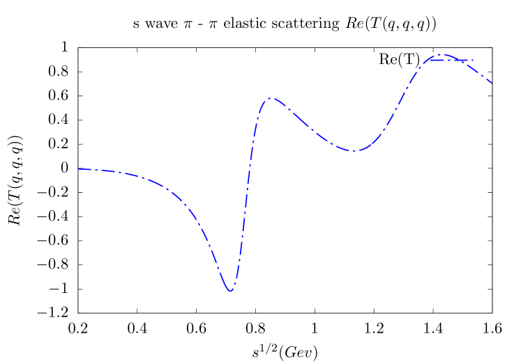
Figure 5: Real part of T

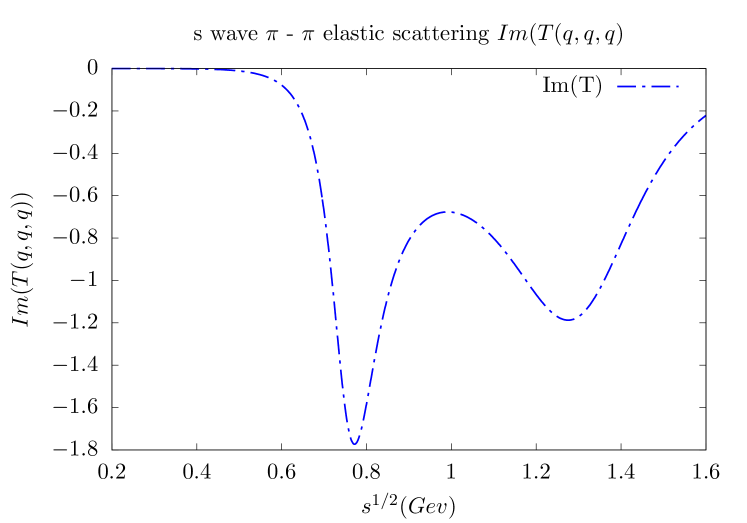
Figure 6: Imaginary part of T

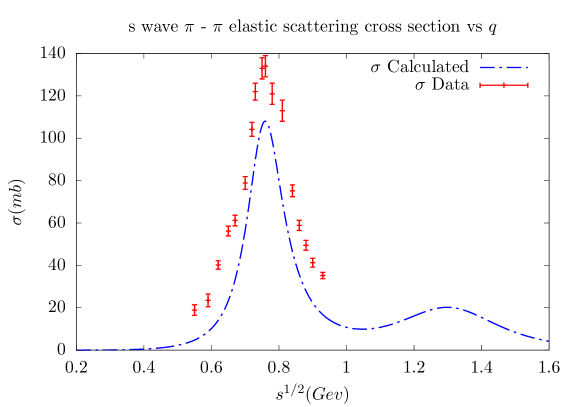
Figure 7: Cross section

IX Unstable particles

Bound states occur when

$$M_{n_{1},n_{2},\kappa_{12}}-M_{n_{0}}>0$$ (171)

for all $n_{1}$ and $n_{2}$. When (171) is negative the denominator in (108) can vanish. When this happens the bound state becomes unstable with respect to decay into the two-bare meson channels. All but a small number of the bare mesons states will fall into this category.

The correct way to understand the resonant behavior is the same way that they are observed experimentally, by looking for peaks in the differential cross section. Equation (167) already has the resonant form exhibiting a complex shift in the position of the bare meson pole.

When perturbation theory is justified, expressions for the lifetime and mass corrections are simple: The expression for the second order correction to the binding energy in (120) becomes complex

$$\int\mspace{-19.0mu}-\sum_{n_{1},n_{2}}q_{12}^{2}dq_{12}{|\langle n_{0}\|v_{1:2}\|n_{1},n_{2},q_{12}\rangle|^{2}\over M_{n_{0}}-M_{n_{1},n_{2},q_{12}}}$$

$$-i\pi\int\delta(M_{n_{0}}-M_{n_{1},n_{2},q_{12}})q_{12}^{2}dq_{12}|\langle n_{1},n_{2},q_{12}\|v_{2:1}\|n_{0}\rangle|^{2}$$ (172)

where $\int\mspace{-19.0mu}-$ indicates a principal value integral. The principal value term gives the leading correction to the bare mass. The imaginary term arises because the bound state can decay to the two-particle continuum. The imaginary part leads to a wave function with an amplitude that decays like

$$e^{-\Gamma t/2}$$ (173)

where $\tau=1/\Gamma$ is the lifetime of the unstable state in perturbation theory:

$$\Gamma=\sum_{\mathbf{n}_{1}\mathbf{n}_{2}}2\pi{q_{120}\omega_{n1}(q_{120})\omega_{n2}(q_{120})\over\omega_{n1}(q_{120})+\omega_{n2}(q_{120})}|\langle n_{1},n_{2},q_{120}|v_{21}|n_{0}\rangle|^{2}$$ (174)

The sum in (174) sum is over the open decay channels which are the channels where

$$M_{{n}_{1},{n}_{2},q_{120}}=M_{{n}_{0}}$$ (175)

has solutions for real $q^{2}_{120}$ that depend on $n_{1}$ and $n_{2}$. This requires

$$M_{{n}_{1},{n}_{2},0}<M_{{n}_{0}}$$ (176)

These solutions are

$${q}_{120}^{2}={M_{{n}_{1}}^{4}+M_{{n}_{2}}^{4}+M_{{n}_{0}}^{4}-2M_{{n}_{1}}^{2}M_{{n}_{2}}^{2}-2M_{{n}_{1}}^{2}M_{{n}_{0}}^{2}-2M_{{n}_{2}}^{2}M_{{n}_{0}}^{2}\over 4M_{{n}_{0}}^{2}}$$ (177)

when the numerator is positive.

Partial widths for decay into the bare mesonic states $n_{1}$ and $n_{2}$ are given by

$$\Gamma_{n_{1},n_{2}}=2\pi{q_{120}\omega_{n1}(q_{120})\omega_{n2}(q_{120})\over\omega_{n1}(q_{120})+\omega_{n2}(q_{120})}|\langle n_{1},n_{2},q_{120}\|v_{21}\|n_{0}\rangle|^{2}$$ (178)

Again, $n_{1}$ and $n_{2}$ represent several quantum numbers.

This perturbative expression is identical to the $\Gamma$ in (157) obtained by looking at the scattering amplitude near resonance, except in the exact case the shift is a function of $\kappa$, so the position of the peak has to be determined by by finding the value of $\kappa$ that makes the real part of denominator of (167) vanish.

This analysis is applied to treat the decay of the $\rho$ meson into a pair of pions. Using the parameters given in section VII, the bare $\rho$ mass is shifted down by $.122$ GeV from its value of $.882$ to the physical value of $.770$ GeV. The resulting width is $\Gamma_{p}=.134\times GeV$ which is qualitatively consistent with the observed width of $.150$ GeV. The size of the resonant shift, 12.7%, is consistent with the size of the 17% correction to the pion mass due to the coupling to the sea quarks in this model. Similar calculation could be performed for higher lying states; these will generally involve more open channels.

X form factors

The last type of observables of interest are electromagnetic observables. Electron scattering from a hadron includes contributions from both valence and sea quarks.

The simplest electron scattering reaction is the scattering of an electron from a charged pion. The relevant observable is the pion form factor. Because the momentum transfer is space-like the form factor can always be calculated in a frame where the $+$ component of the momentum transfer is zero, $Q^{+}=0$. The form factor can be expressed in terms of the $+$ component of the current at $x=0$:

$$F_{\pi}(Q^{2})=\langle\pi,\tilde{\mathbf{p}}^{\prime}|I^{+}(0)|\pi,\tilde{\mathbf{p}}\rangle$$ (179)

where the pion state (in this model) will in general include both valence and sea quark contributions. In this model the pion state vector has the form

$$\left(\begin{array}[]{c}|\pi,\mathbf{\tilde{p}}\rangle_{1}\\ {1\over m_{\pi}-M_{2}}v_{2:1}{1\over m_{\pi}-M_{1}}|\pi,\mathbf{\tilde{p}}\rangle_{1}\\ \end{array}\right)$$ (180)

where $m_{\pi}$ is the mass eigenvalue. The current matrix element has the general form

$$\langle\pi,\mathbf{p}_{\perp}^{\prime}|I^{+}(0)|\pi,\mathbf{p}_{\perp}\rangle=$$

$${}_{1}\langle\pi,\mathbf{\tilde{p}}^{\prime}|I^{\mu}(0)|\pi,\mathbf{\tilde{p}}\rangle_{1}+$$

$${}_{1}\langle\pi,\mathbf{\tilde{p}}^{\prime}|I^{\mu}(0)|{1\over m_{\pi}-M_{2}}v_{2:1}{1\over m_{\pi}-M_{1}}|\pi,\mathbf{\tilde{p}}\rangle_{1}+$$

$${}_{1}\langle\pi,\mathbf{\tilde{p}}|{1\over m_{\pi}-M_{1}}v_{12}{1\over m_{\pi}-M_{2}}|I^{\mu}(0)|\pi,\mathbf{\tilde{p}}\rangle_{1}+$$

$${}_{1}\langle\pi,\mathbf{\tilde{p}}|{1\over m_{\pi}-M_{1}}v_{12}{1\over m_{\pi}^{*}-M_{2}}|I^{\mu}(0)|{1\over m_{\pi}^{*}-M_{2}}v_{2:1}{1\over m_{\pi}-M_{1}}|\pi,\mathbf{\tilde{p}}^{\prime}\rangle_{1}$$ (181)

This expression involves both the wave functions and current operators. The evaluation of the current matrix elements is naturally performed in the quark-anti-quark-gluon representation. The advantage of the light front representation is invariance of the single quark magnetic quantum numbers under light front boosts, which lead to frame-independent impulse approximations. In addition the boosts are kinematic. On the other hand the quark current operator necessarily has many-body contributions due to the dynamical nature of rotational covariance and current conservation. These relations involve the string breaking vertex.

The structure of the full current is beyond the scope of this model. It is nevertheless useful to examine the pion form factor assuming that the quarks can be treated a point particles in the valence sector of this model to determine if there is any kind of qualitative agreement with experiment.

Equation (181) can be interpreted as the matrix element of a two-body current in the valence state, however in this case valence state is not the same as the bare state, and there is an additional normalization correction that appears in the current.

The simplest calculation is the calculation of the charge form factor for the bare pion assuming that the single quark and anti-quark are treated as point charges with no magnetic form factors. In this case the pion form factor is given by the first term in (181) where the valence wave function is replaced by the bare wave function. The results of the calculation are shown in figures 8 and 9, where they are compared to low and high energy data from Amendolia et al. (1986)Volmer et al. (2001)Bebek et al. (1978). The solid curves use the quark masses and oscillator parameters of this model. The dash-dot curves use an oscillator wave function with $\lambda=.259$ and quark masses of $m_{q}=.20$, which were the values used in Coester and Polyzou (2005), and the dotted curves use $\lambda=.282$ and $m_{q}=.2$.

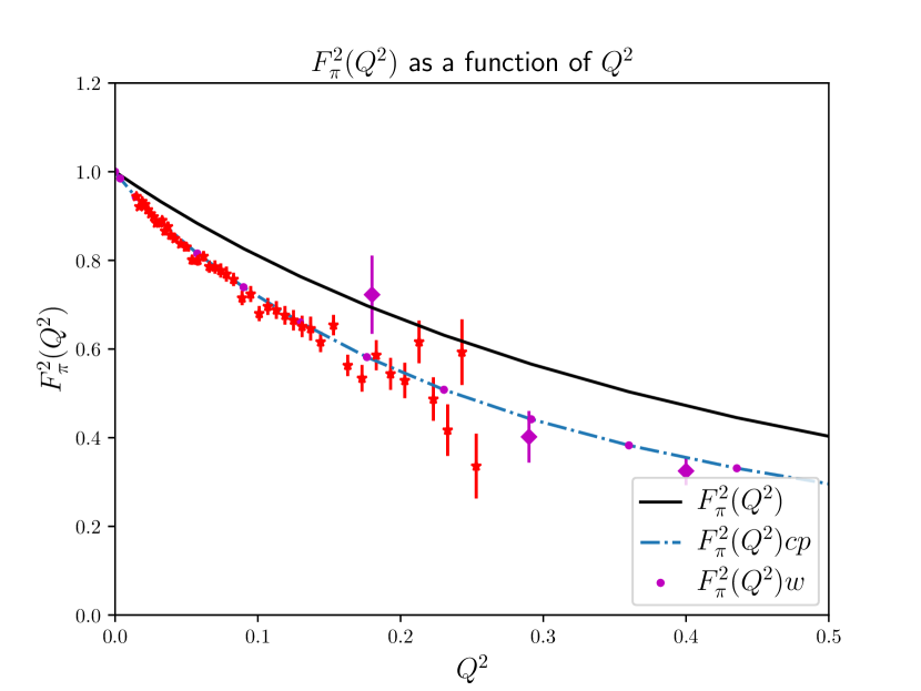
Figure 8: $F_{\pi}(Q^{2})$

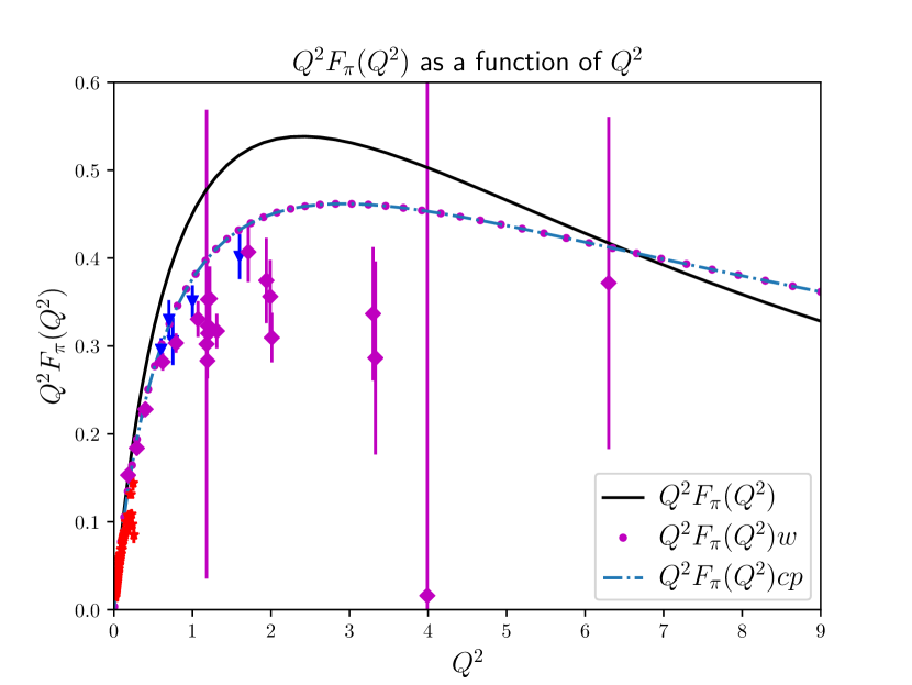
Figure 9: $Q^{2}F_{\pi}(Q^{2})$

The single quark and anti-quarks are treated as point charges with no magnetic form factors. Equation (93) is used to express the valence wave function in terms of the single quark degrees of freedom. The calculated form factor is too large compared to data for both low and high $Q^{2}$, however a rough agreement was achieved in Coester and Polyzou (2005) using the same valence wave function with $\lambda$ decreased by about 8% to .259 and a lighter quark mass, $m=.2$ . Since the quark masses appear in the Poincaré generators in the in the combination $m_{q}^{2}+V_{0}$, there is an additional freedom to reduce the quark masses keeping $m_{q}^{2}+V_{0}$ constant. This freedom leaves the Poincaré generators unchanged. It leaves the bound state, scattering, and lifetime calculations unchanged. Reducing the quark masses to $m_{q}=.2$ without changing the coupling constant gives the curves with the dots, which are indistinguishable from the results of Coester and Polyzou (2005) which use a slightly reduced value of $\lambda$. Further calculations are needed to determine the corrections due to sea quarks and two-body currents.

XI conclusion

This work examined a simple model of mesons, based on non-local degrees of freedom that are both globally and locally gauge invariant. The structure of the model was largely motivated by the strong coupling limit of Hamiltonian lattice QCD. Gauge invariant systems of quarks and anti-quarks connected by links were modeled by quark anti-quark pairs interacting via a confining interaction. A key feature is that quarks in different connected singlets are treated as distinguishable particles. The model has dual representations in terms of hadronic and QCD degrees of freedom. While there are many possible interactions involving connected gauge invariant degrees of freedom, this work examined the consequence of the assumption that the dominant contribution comes from string breaking, which produces quark-anti-quark pairs from a given local/global singlet state. The model was formulated so all matrix elements of the string breaking vertex with bare meson states could be computed analytically in terms of the underlying QCD degrees of freedom. Calculations were performed by truncating to the direct sum of a one and two-singlet subspace. The model is formulated to be fully relativistic and designed so computations can be performed efficiently. In order to stay close in spirit to QCD, one parameter was used to set all of the scales. In this application that parameter was fixed by the Regge slope of the family of excitations of the $\rho$ meson in the valence model, which fixed a confinement scale. The same parameter was used to fix the size of the string breaking vertex, however a scale transformation on the string breaking vertex was needed to get a qualitatively consistent treatment of lifetimes and spectral properties. The vertex also included a dimensionless coupling constant of order unity. The model was used to calculate sea quark contributions to bound states, spectral properties, cross sections, lifetimes and electromagnetic properties. The calculations of spectral properties, lifetimes, and scattering cross sections generally gave results that were qualitatively consistent with experiment. The calculation were consistent with a non-trivial sea quark component in the pion state vector. The pion form factor in the bare model over predicted the experimental data for both high and low momentum transfers, however the data can be fit with the same wave functions using smaller quark masses (48%). Since the quark mass in this model appears in the combination $m_{q}^{2}+V_{0}$, it could be reduced by changing $V_{0}$ to keep this combination constant. This change leaves all of the dynamical operators unchanged, so would not affect the bound state, scattering or resonance calculations. Further adjustments in the quark masses are anticipated after contributions from sea quarks or two-body currents are included.

These results suggest that a string breaking reaction mechanism is a significant component of hadronic dynamics, and could provide a good starting point for developing more realistic models of hadronic dynamics. This type of model could also be extended to treat baryons modeled as diquarks, which would provide more stringent experimental constraints. This model is also directly applicable to treating exotic mesons as confined diquark-anti-diquark systems, or as molecules of confined quark and anti-quarks. Realistic applications require generalizing the model to include flavor dependent interactions.

This research supported by the US Department of Energy, Office of Science, grant number DE-SC0016457 who supported this research effort.

XII Appendix I: String breaking matrix elements

In this and the next appendix the analytic expression (72) for the matrix elements of spin-independent part of the string breaking vertex the oscillator basis is derived. This involves a 9 dimensional integral that can be computed analytically.

In order to calculate matrix elements of this vertex with the harmonic oscillator states the expressions for the smeared delta functions are inserted in the expression for the vertex. The resulting expression for the kernel of the string-breaking vertex becomes

$$\langle\mathbf{r}_{1},\mathbf{r}_{2},\mathbf{r}_{12}|v_{2:1}|\mathbf{r}\rangle:=$$

$${g\over\sqrt{\lambda}}\delta(\mathbf{r}-2\mathbf{r}_{12})({\lambda\over 4\pi})^{3}\int_{0}^{1}d\eta e^{-{\lambda\over 4}((\mathbf{r}_{1}-2\eta\mathbf{r}_{12})^{2}+(\mathbf{r}_{2}-2(1-\eta)\mathbf{r}_{12})^{2})}$$ (182)

where the Gaussians delta functions are expressed using

$$e^{-{\lambda\over 4}(\mathbf{r}_{i}-2\alpha\mathbf{r}_{12})^{2}}=e^{-{\lambda\over 4}\mathbf{r}_{i}^{2}-\lambda\alpha^{2}\mathbf{r}_{12}^{2}+\alpha\lambda\mathbf{r}_{i}\cdot\mathbf{r}_{12}}.$$ (183)

The angle dependent part of (183) can be represented using the partial-wave expansion of $e^{\mathbf{k}\cdot\mathbf{x}}$ Abramowitz and Stegun (1964) (see section 10.2.36 page 445 - which is the analytic continuation of the usual expansion of plane waves in spherical harmonics:)

$$e^{i\mathbf{k}\cdot\mathbf{r}}=4\pi\sum l^{l}j_{l}(kr)Y^{*}_{lm}(\hat{\mathbf{k}})Y_{lm}(\hat{\mathbf{r}})$$ (184)

which becomes

$$e^{z\cos(\theta)}=\sum_{n=0}^{\infty}(2n+1)\sqrt{\pi\over 2z}I_{n+1/2}(z)P_{n}(\cos(\theta))$$ (185)

or

$$e^{\alpha\lambda\mathbf{r}_{i}\cdot\mathbf{r}_{12}}=4\pi\sqrt{{\pi\over 2\lambda\alpha r_{i}r_{12}}}\sum_{l=0}^{\infty}\sum_{m=-l}^{l}I_{l+{1\over 2}}(\lambda\alpha r_{i}r_{12})Y^{*}_{lm}(\hat{\mathbf{r}_{i}})Y_{lm}(\hat{\mathbf{r}_{12}}).$$ (186)

The Bessel function $I_{l+{1\over 2}}(2ab)$ in (186) is a generating function for the associated Laguerre polynomials (see Abramowitz and Stegun (1964), equations 22.9.16 and 9.6.3 or Schwinger and Englert (2001) problem 7.12). Abramowitz and Stegun give the following expressions

$$(xz)^{-\alpha/2}e^{z}J_{\alpha}(2(xz)^{1/2})=\sum_{n=0}^{\infty}L^{\alpha}_{n}(x){z^{n}\over\Gamma(n+a+1)}$$ (187)

$$I_{\nu}(z)=e^{-{1\over 2}\nu\pi i}J_{\nu}(ze^{{1\over 2}\pi i})\qquad-\pi<\phi<\pi/2$$ (188)

$$I_{\nu}(z)=e^{{3\over 2}\nu\pi i}J_{\nu}(ze^{-{3\over 2}\pi i})\qquad\pi/2<\phi<\pi$$ (189)

and Schwinger gives (problem 7.12 p. 302) the equivalent but more useful expression

$$e^{-\lambda}I_{\alpha}(2\sqrt{\lambda x})=(\lambda x)^{\alpha\over 2}\sum_{n=0}^{\infty}(-)^{n}{\lambda^{n}\over(n+\alpha)!}L^{\alpha}_{n}(x)$$ (190)

which in this case is

$$I_{l+{1\over 2}}(2ab)=e^{a^{2}}(ab)^{l+{1\over 2}}\sum_{n=0}^{\infty}(-)^{n}{a^{2n}\over\Gamma(n+l+{3\over 2})}L_{n}^{l+{1\over 2}}(b^{2}).$$ (191)

In what follows this expression is used with $a=\sqrt{{\lambda\over 2}}\alpha r_{12}$ and $b=\sqrt{{\lambda\over 2}}r_{i}$.

Using (191) in (186) along with the expression (51) for the harmonic oscillator wave function gives

$$e^{-{\lambda\over 4}(\mathbf{r}_{i}-2\alpha\mathbf{r}_{12})^{2}}=$$

$$2\pi^{3/2}\sum_{n,l,m}(\sqrt{{\lambda\over 2}}\alpha r_{12})^{2n+l}e^{-{\lambda\over 2}\alpha^{2}r_{12}^{2}}(-)^{n}{(\sqrt{{\lambda\over 2}}r_{i})^{l}L^{l+{1\over 2}}_{n}({\lambda\over 2}r_{i}^{2})e^{-{\lambda\over 4}r_{i}^{2}}\over\Gamma(n+l+{3\over 2})}Y_{lm}(\hat{\mathbf{r}}_{i})Y^{*}_{lm}(\hat{\mathbf{r}_{12}})=$$

$$2\pi^{3/2}({2\over\lambda})^{3/4}e^{-{\lambda\over 2}\alpha^{2}r_{12}^{2}}\sum_{n=0}^{\infty}(\sqrt{{\lambda\over 2}}\alpha r_{12})^{2n+l}{R_{nl}({r}_{i})\over\sqrt{2n!\Gamma(n+l+{3\over 2})}}Y_{lm}(\hat{\mathbf{r}_{i}})Y_{lm}^{*}(\hat{\mathbf{r}_{12}})$$ (192)

where this has been expressed in terms of the radial harmonic oscillator wave function $R_{nl}(r)$.

Letting $\alpha=\eta$ and $\alpha=1-\eta$ gives the following expression for the kernel of the vertex as an expansion in harmonic oscillator states:

$$\langle\mathbf{r}_{1},\mathbf{r}_{2},\mathbf{r}_{12}|v_{2:1}|\mathbf{r}\rangle=$$

$${g\over\sqrt{\lambda}}\delta(\mathbf{r}-2\mathbf{r}_{12})({\lambda\over 4\pi})^{3}4\pi^{3}({2\over\lambda})^{3/2}\sum_{n_{1}l_{1}m_{1}n_{2}l_{2}m_{2}}\int_{0}^{1}d\eta e^{-{\lambda\over 2}{r}_{12}^{2}(\eta^{2}+(1-\eta)^{2})}\eta^{l_{1}+2n_{1}}(1-\eta)^{l_{2}+2n_{2}}\times$$

$$(\sqrt{{\lambda\over 2}}{r}_{12})^{2n_{1}+l_{1}+2n_{2}+l_{2}}{\psi_{n_{1}l_{1}m_{1}}({\mathbf{r}}_{1})Y^{*}_{l_{1}m_{1}}(\hat{\mathbf{r}}_{12})\psi_{n_{2}l_{2}m_{2}}({\mathbf{r}}_{2})Y^{*}_{l_{2}m_{2}}(\hat{\mathbf{r}}_{12})\over\sqrt{2n_{1}!\Gamma(n_{1}+l_{1}+{3\over 2})}\sqrt{2n_{2}!\Gamma(n_{2}+l_{2}+{3\over 2})}}$$ (193)

where

$$\psi_{nlm}(\mathbf{r})=R_{nl}(\mathbf{r})Y_{lm}(\hat{\mathbf{r}}).$$ (194)

Integrating this against three oscillator eigenstates in $\mathbf{r}_{1}$, $\mathbf{r}_{2}$ and $\mathbf{r}$ reduces the vertex in coordinate space to an expression in terms of a single one-dimensional integral

$$\langle n_{1},l_{1},m_{1},n_{2},l_{2},m_{2},\mathbf{r}_{12}|v_{2:1}|n,l,m\rangle=\int\psi_{n_{1}l_{1}m_{1}}^{*}(\mathbf{r}_{1})\psi_{n_{2}l_{2}m_{2}}^{*}(\mathbf{r}_{2})v(\mathbf{r}_{1},\mathbf{r}_{2},\mathbf{r}_{12};\mathbf{r})\psi_{nlm}(\mathbf{r})d\mathbf{r}_{1}d\mathbf{r}_{2}d\mathbf{r}$$

$$={g\over\sqrt{\lambda}}R_{nl}(2{r}_{12})({2\lambda})^{3/2}{(\sqrt{{\lambda\over 2}}{r}_{12})^{2n_{1}+l_{1}+2n_{2}+l_{2}}\over(\sqrt{2n_{1}!\Gamma(n_{1}+l_{1}+{3\over 2}})(\sqrt{2n_{2}!\Gamma(n_{2}+l_{2}+{3\over 2}})}\times$$

$$\int_{0}^{1}d\eta e^{-{\lambda\over 2}{r}_{12}^{2}(\eta^{2}+(1-\eta)^{2})}\eta^{l_{1}+2n_{1}}(1-\eta)^{l_{2}+2n_{2}}Y_{lm}(\hat{\mathbf{r}}_{12})Y_{l_{1}m_{1}}^{*}(\hat{\mathbf{r}}_{12})Y_{l_{2}m_{2}}^{*}(\hat{\mathbf{r}}_{12}).$$ (195)

The one-dimensional integral

$$\int_{0}^{1}d\eta e^{-{\lambda\over 2}r_{12}^{2}(\eta^{2}+(1-\eta)^{2})}\eta^{l_{1}+2n_{1}}(1-\eta)^{l_{2}+2n_{2}}$$ (196)

can be performed analytically, although a numerical calculation may be more efficient. The analytic calculation is given in appendix II. The result of this calculation is

$$\int_{0}^{1}d\eta e^{-{\lambda\over 2}r_{12}^{2}(\eta^{2}+(1-\eta)^{2})}\eta^{l_{1}+2n_{1}}(1-\eta)^{l_{2}+2n_{2}}=e^{-{\lambda\over 4}{r}_{12}^{2}}\int_{0}^{1}d\eta e^{-\lambda r_{12}^{2}(\eta-{1\over 2})^{2}}\eta^{2n_{1}+l_{1}}(1-\eta)^{2n_{2}+l_{2}}$$

$$=e^{-{\lambda\over 4}r_{12}^{2}}\sum_{k_{1}+k_{2}=2r}{(l_{1}+2n_{1})!(l_{2}+2n_{2})!\over k_{1}!k_{2}!(l_{1}+2n_{1}-k_{1})!(l_{2}+2n_{2}-k_{2})!}(-)^{k_{2}}({1\over 2})^{l_{1}+2n_{1}+l_{2}+2n_{2}}\times$$

$${1\over 2r+1}M({1\over 2}+r,{3\over 2}+r,-{\lambda r^{2}_{12}\over 4})$$ (197)

where the sum is over $k_{1}$, and $k_{2}$ keeping only terms with $k_{1}+k_{2}=2r$ even, $0\leq k_{i}\leq 2n_{i}+l_{i}$, and $M(\alpha,\beta,\gamma)$ is the confluent hypergeometric function.

The kernel of the spin-independent part of the string breaking vertex is

$$\langle n_{1},l_{1},m_{1},n_{2},l_{2},m_{2},\mathbf{r}_{12}|v_{2:1}|n,l,m\rangle=$$

$$\int\psi_{n_{1}l_{1}m_{1}}^{*}(\mathbf{r}_{1})\psi_{n_{2}l_{2}m_{2}}^{*}(\mathbf{r}_{2})v(\mathbf{r}_{1},\mathbf{r}_{2},\mathbf{r}_{12};\mathbf{r})\psi_{nlm}(\mathbf{r})d\mathbf{r}_{1}d\mathbf{r}_{2}d\mathbf{r}=$$

$${g\over\sqrt{\lambda}}R_{nl}(2{r}_{12})({2\lambda})^{3/2}{(\sqrt{{\lambda\over 2}}{r}_{12})^{2n_{1}+l_{1}+2n_{2}+l_{2}}\over\sqrt{2n_{1}!\Gamma(n_{1}+l_{1}+{3\over 2}})\sqrt{2n_{2}!\Gamma(n_{2}+l_{2}+{3\over 2}})}\times$$

$$e^{-{\lambda\over 4}r_{12}^{2}}\sum_{k_{1}+k_{2}=2r}{(l_{1}+2n_{1})!(l_{2}+2n_{2})!\over k_{1}!k_{2}!(l_{1}+2n_{1}-k_{1})!(l_{2}+2n_{2}-k_{2})!}(-)^{k_{2}}({1\over 2})^{l_{1}+2n_{1}+l_{2}+2n_{2}}\times$$

$${1\over 2r+1}M({1\over 2}+r,{3\over 2}+r,-{\lambda r^{2}_{12}\over 4})Y_{lm}(\hat{\mathbf{r}}_{12})Y_{l_{1}m_{1}}^{*}(\hat{\mathbf{r}}_{12})Y_{l_{2}m_{2}}^{*}(\hat{\mathbf{r}}_{12}).$$ (198)

The radial part of this expression is the part of (198) that multiplies the three spherical harmonics:

$$\langle n_{1},l_{1},n_{2},l_{2},{r}_{12}|v_{2:1}|n,l\rangle=$$

$${g\over\sqrt{\lambda}}R_{nl}(2{r}_{12})({2\lambda})^{3/2}\times$$

$${(\sqrt{{\lambda\over 2}}{r}_{12})^{2n_{1}+l_{1}+2n_{2}+l_{2}}\over\sqrt{2n_{1}!\Gamma(n_{1}+l_{1}+{3\over 2}})\sqrt{2n_{2}!\Gamma(n_{2}+l_{2}+{3\over 2}})}\times$$

$$e^{-{\lambda\over 4}r_{12}^{2}}\sum_{k_{1}+k_{2}=2r}{(l_{1}+2n_{1})!(l_{2}+2n_{2})!\over k_{1}!k_{2}!(l_{1}+2n_{1}-k_{1})!(l_{2}+2n_{2}-k_{2})!}(-)^{k_{2}}({1\over 2})^{l_{1}+2n_{1}+l_{2}+2n_{2}}\times$$

$${1\over 2r+1}M({1\over 2}+r,{3\over 2}+r,-{\lambda r^{2}_{12}\over 4}).$$ (199)

XIII Appendix II

The integral (196) that must be evaluated in Appendix I to get an analytic expression for the meson form factors in the coordinate representation has the form

$$I_{n_{1}.l_{1},n_{2},l_{2}}(r_{12})=$$

$$\int_{0}^{1}e^{-{\lambda\over 2}r_{12}^{2}(\eta^{2}+\eta^{2}-2\eta+1}\eta^{l_{1}+2n_{1}}(1-\eta)^{l_{2}+2n_{2}}d\eta=$$

$$e^{-{\lambda\over 4}r_{12}^{2}}\int_{0}^{1}e^{-{\lambda}r_{12}^{2}(\eta-{1\over 2})^{2}}\eta^{l_{1}+2n_{1}}(1-\eta)^{l_{2}+2n_{2}}d\eta.$$ (200)

Let $\nu=\eta-{1\over 2}$ so this becomes

$$I_{n_{1}.l_{1},n_{2},l_{2}}(r_{12})=e^{-{\lambda\over 4}r_{12}^{2}}\int_{-{1\over 2}}^{{1\over 2}}e^{-{\lambda}r_{12}^{2}\nu^{2}}({1\over 2}+\nu)^{l_{1}+2n_{1}}({1\over 2}-\nu)^{l_{2}+2n_{2}}d\nu.$$ (201)

Using the binomial theorem this becomes

$$I_{n_{1}.l_{1},n_{2},l_{2}}(r_{12})=$$

$$=e^{-{\lambda\over 4}r_{12}^{2}}\sum_{k_{1}+k_{2}=2r}{(l_{1}+2n_{1})!(l_{2}+2n_{2})!\over k_{1}!k_{2}!(l_{1}+2n_{1}-k_{1})!(l_{2}+2n_{2}-k_{2})!}(-)^{k_{2}}({1\over 2})^{l_{1}+2n_{1}+l_{2}+2n_{2}-2r}\int_{-{1\over 2}}^{{1\over 2}}e^{-{\lambda}r_{12}^{2}\nu^{2}}\nu^{2r}=$$

$$=e^{-{\lambda\over 4}r_{12}^{2}}\sum_{k_{1}+k_{2}=2r}{(l_{1}+2n_{1})!(l_{2}+2n_{2})!\over k_{1}!k_{2}!(l_{1}+2n_{1}-k_{1})!(l_{2}+2n_{2}-k_{2})!}(-)^{k_{2}}({1\over 2})^{l_{1}+2n_{1}+l_{2}+2n_{2}-2r}\times$$

$$(-{1\over r_{12}^{2}})^{r}{d^{r}\over d\lambda^{r}}\int_{-{1\over 2}}^{{1\over 2}}e^{-{\lambda}r_{12}^{2}\nu^{2}}$$

$$=e^{-{\lambda\over 4}r_{12}^{2}}\sum_{k_{1}+k_{2}=2r}{(l_{1}+2n_{1})!(l_{2}+2n_{2})!\over k_{1}!k_{2}!(l_{1}+2n_{1}-k_{1})!(l_{2}+2n_{2}-k_{2})!}(-)^{k_{2}}({1\over 2})^{l_{1}+2n_{1}+l_{2}+2n_{2}-2r}\times$$

$$(-{1\over r_{12}^{2}})^{r}{d^{r}\over d\lambda^{r}}{1\over\sqrt{\lambda}r_{12}}\int_{-{\sqrt{\lambda}r_{12}\over 2}}^{{\sqrt{\lambda}r_{12}\over 2}}e^{-\rho^{2}}d\rho.$$ (202)

Next express the integral in terms of the error function

$$\mbox{erf}(z)={2\over\sqrt{\pi}}\int_{0}^{z}e^{-t^{2}}dt$$ (203)

to get

$$I_{n_{1}.l_{1},n_{2},l_{2}}(r_{12})=$$

$$=e^{-{\lambda\over 4}r_{12}^{2}}\sum_{k_{1}+k_{2}=2r}{(l_{1}+2n_{1})!(l_{2}+2n_{2})!\over k_{1}!k_{2}!(l_{1}+2n_{1}-k_{1})!(l_{2}+2n_{2}-k_{2})!}(-)^{k_{2}}({1\over 2})^{l_{1}+2n_{1}+l_{2}+2n_{2}-2r}\times$$

$${\sqrt{\pi}\over 4}(-{1\over r_{12}^{2}})^{r}{d^{r}\over d\lambda^{r}}{2\over\sqrt{\lambda}r_{12}}\left({2\over\sqrt{\lambda}r_{12}}\mbox{erf}({\sqrt{\lambda}r_{12}\over 2})-{2\over\sqrt{\lambda}r_{12}}\mbox{erf}(-{\sqrt{\lambda}r_{12}\over 2})\right)$$ (204)

then express the error functions in terms of confluent hypergeometric function (see AS 7.1.21)

$${\mbox{erf}(z)\over z}={2\over\sqrt{\pi}}M({1\over 2},{3\over 2},-z^{2})$$ (205)

$$I_{n_{1}.l_{1},n_{2},l_{2}}(r_{12})=$$

$$=e^{-{\lambda\over 4}r_{12}^{2}}\sum_{k_{1}+k_{2}=2r}{(l_{1}+2n_{1})!(l_{2}+2n_{2})!\over k_{1}!k_{2}!(l_{1}+2n_{1}-k_{1})!(l_{2}+2n_{2}-k_{2})!}(-)^{k_{2}}({1\over 2})^{l_{1}+2n_{1}+l_{2}+2n_{2}-2r}\times$$

$${\sqrt{\pi}\over 4}(-{1\over r_{12}^{2}})^{r}{d^{r}\over d\lambda^{r}}{2\over\sqrt{\lambda}r_{12}}\left({2\over\sqrt{\pi}}M({1\over 2},{3\over 2},-{\lambda r^{2}_{12}\over 4})+{2\over\sqrt{\pi}}M({1\over 2},{3\over 2},-{\lambda r^{2}_{12}\over 4})\right)$$

$$=e^{-{\lambda\over 4}r_{12}^{2}}\sum_{k_{1}+k_{2}=2r}{(l_{1}+2n_{1})!(l_{2}+2n_{2})!\over k_{1}!k_{2}!(l_{1}+2n_{1}-k_{1})!(l_{2}+2n_{2}-k_{2})!}(-)^{k_{2}}({1\over 2})^{l_{1}+2n_{1}+l_{2}+2n_{2}-2r}\times$$

$${1\over 4^{r}}{d^{r}\over d(-\lambda r_{12}^{2}/4)^{r}}{2\over\sqrt{\lambda}r_{12}}M({1\over 2},{3\over 2},-{\lambda r^{2}_{12}\over 4}).$$ (206)

Next use AS 13.4.9 to express derivatives of the confluent hypergeometric functions in terms of the confluent function.

$$I_{n_{1}.l_{1},n_{2},l_{2}}(r_{12})=$$

$$=e^{-{\lambda\over 4}r_{12}^{2}}\sum_{k_{1}+k_{2}=2r}{(l_{1}+2n_{1})!(l_{2}+2n_{2})!\over k_{1}!k_{2}!(l_{1}+2n_{1}-k_{1})!(l_{2}+2n_{2}-k_{2})!}(-)^{k_{2}}({1\over 2})^{l_{1}+2n_{1}+l_{2}+2n_{2}-2r}\times$$

$${1\over 4^{r}}{\Gamma({1\over 2}+r)\Gamma({3\over 2})\over\Gamma({3\over 2}+r)\Gamma({1\over 2})}M({1\over 2}+r,{3\over 2}+r,-{\lambda r^{2}_{12}\over 4})$$

which gives (197)

$$=e^{-{\lambda\over 4}r_{12}^{2}}\sum_{k_{1}+k_{2}=2r}{(l_{1}+2n_{1})!(l_{2}+2n_{2})!\over k_{1}!k_{2}!(l_{1}+2n_{1}-k_{1})!(l_{2}+2n_{2}-k_{2})!}(-)^{k_{2}}({1\over 2})^{l_{1}+2n_{1}+l_{2}+2n_{2}}\times$$

$${1\over 2r+1}M({1\over 2}+r,{3\over 2}+r,-{\lambda r^{2}_{12}\over 4}).$$ (207)

XIV Appendix III: Cook Condition

If the vertex is evaluated by projecting on a truncated basis the resulting interaction is separable. While the separable approximation is a short-range compact interaction which has a non-trivial scattering operator, it is not automatically true that the sum of an infinite number of separable terms remains short ranged. For this reason it is desirable to prove that the limit of the $S$ matrix with truncated numbers of channels converges in the infinite number of channel limit to the exact $S$-matrix. Here exact means in the context of the $2+1$ singlet model.

On way to avoid directly dealing with infinite number of channels is to show the existence of the channel wave operators that are used to make the $S$ operator. The Cook condition Cook (1957) is a sufficient condition for the strong convergence of the time limits that define scattering wave operators

$$\Omega_{\pm n_{1}n_{2}}:=\lim_{\tau\to\pm\infty}e^{iM\tau}\Phi_{n_{1}n_{2}}e^{-iM_{n_{1}n_{2}}\tau}|f_{1}f_{2}\rangle$$ (208)

for and initial or final state in the $n_{1},n_{2}$ two meson channel.

For the model of section VI the Cook condition is

$$\int_{c}^{\pm\infty}\|v_{1:2}\Phi_{n_{1}n_{1}}e^{-iM_{n_{1}n_{1}}\tau}|f_{1}f_{2}\rangle\|d\tau<\infty.$$ (209)

To show that this inequality is satisfied it is necessary to show that

$$\|v_{1:2}\Phi_{n_{1}n_{1}}e^{-iM_{n_{1}n_{1}}\tau}|f_{1}f_{2}\rangle\|$$ (210)

is an integrable function of $\tau$ for a dense set of initial or final wave packets.

The Cook condition follows provided that the square of (210) has the form

$$\int d\mathbf{r}_{12}f^{*}(\mathbf{r}_{12},\tau)K^{*}(\mathbf{r}_{12})K(\mathbf{r}_{12})f(\mathbf{r}_{12},\tau)d\mathbf{r}_{12}$$ (211)

where $\int|K(\mathbf{r}_{12})|^{2}d\mathbf{r}_{12}$ is finite and $f(\mathbf{r}_{12},\tau)$ satisfies

$$|f(\mathbf{r},2\tau)|<{c_{1}\over c_{2}+\tau^{3/2}}$$ (212)

for constants $c_{1}$ and $c_{2}$. This ensures that the integrand in (209) is bounded by

$$\sqrt{\int|K(\mathbf{r}_{12})|^{2}d\mathbf{r}_{12}}|<{c_{1}\over c_{2}+\tau^{3/2}}$$ (213)

which is integrable.

In what follows only the simplest case of identical particle scattering is discussed. In this case $M_{n_{1}n_{2}}$ has the form $2\sqrt{m_{n}^{2}+\mathbf{q}^{2}}$ and after factoring out the conserved light-front 3-momentum, the term $\langle\mathbf{r}_{12}|e^{-iM_{n_{1}n_{2}}\tau}|f_{1}f_{2}\rangle$ becomes

$$\langle\mathbf{r}_{12}|e^{-iM_{n_{1}n_{2}}\tau}|f_{1}f_{2}\rangle:={1\over(2\pi)^{3/2}}\int e^{-i2\sqrt{\mathbf{q}^{2}+m_{n}^{2}}\tau+i\mathbf{q}\cdot\mathbf{r}}d\mathbf{q}f(\mathbf{q}).$$ (214)

This has the form of a positive energy solution of the Klein-Gordon equation with a wave packet $f(\mathbf{q})$ in the relative momentum. When $f(\mathbf{q})$ a Schwartz test function these solutions are known to satisfy the bound (212) Ruelle (1962)Jost (1965)Bogoliubov and Shirkov (1959) .

What remains is to verify $\int|K(\mathbf{r}_{12})|^{2}d\mathbf{r}_{12}<\infty$

To construct the kernel $K(\mathbf{r}_{12})$ note that

$$K^{*}(\mathbf{r}_{12})K(\mathbf{r}_{12})=\gamma^{2}\int\delta(\mathbf{r}-2\mathbf{r}_{12})\delta(\mathbf{r}-2\mathbf{r}_{12}^{\prime})d\mathbf{r}_{1}d\mathbf{r}_{2}d\mathbf{r}_{1}^{\prime}d\mathbf{r}_{2}^{\prime}d\mathbf{r}d\mathbf{r}_{12}^{\prime}d\eta d\eta^{\prime}\times$$

$$g(\mathbf{r}_{1}-\eta\mathbf{r})g(\mathbf{r}_{2}-(1-\eta)\mathbf{r})\langle\phi_{n}|\mathbf{r}_{1}\rangle\langle\phi_{n}|\mathbf{r}_{2}\rangle\langle\mathbf{r}^{\prime}_{2}|\phi_{n}\rangle\langle\mathbf{r}^{\prime}_{1}|\phi_{n}\rangle g(\mathbf{r}^{\prime}_{1}-\eta^{\prime}\mathbf{r})g(\mathbf{r}^{\prime}_{2}-(1-\eta^{\prime})\mathbf{r})$$ (215)

The integrals over the delta functions give a factor of ${1\over 2}$ and replace $\mathbf{r}/2=\mathbf{r}_{12}^{\prime}$ by $\mathbf{r}_{12}$. This gives

$$K^{*}(\mathbf{r}_{12})K(\mathbf{r}_{12})={\gamma^{2}\over 2}\int_{0}^{1}d\eta\int_{0}^{1}d\eta^{\prime}$$

$$\int d\mathbf{r}_{1}g(\mathbf{r}_{1}-2\eta\mathbf{r}_{12})\langle\phi_{n}|\mathbf{r}_{1}\rangle\int d\mathbf{r}_{2}g(\mathbf{r}_{2}-2(1-\eta)\mathbf{r}_{12})\langle\phi_{n}|\mathbf{r}_{2}\rangle$$

$$\int d\mathbf{r}_{1}^{\prime}\langle\mathbf{r}^{\prime}_{2}|\phi_{n}\rangle g(\mathbf{r}^{\prime}_{1}-2\eta^{\prime}\mathbf{r}_{12})\int d\mathbf{r}_{2}^{\prime}g(\mathbf{r}^{\prime}_{2}-2(1-\eta^{\prime})\mathbf{r}_{12})\langle\mathbf{r}^{\prime}_{1}|\phi_{n}\rangle$$ (216)

Ignoring the $\eta$ and $\eta^{\prime}$ which are over the compact interval $[0,1]$, this expression is a product of four integrals of identical structure. It is enough to consider one of them; for example

$$\int d\mathbf{r}_{1}g(\mathbf{r}_{1}-2\eta\mathbf{r}_{12})\langle\mathbf{r}_{1}|\phi_{n}\rangle.$$ (217)

In this case $g(\mathbf{r}_{1}-2\eta\mathbf{r}_{12})$ is a Gaussian and the oscillator function, $\langle\phi_{n}|\mathbf{r}_{1}\rangle$, is a Gaussian multiplied by a polynomial. In what follows it will be shown that the result of the integration over $\mathbf{r}_{i}$ is a Gaussian multiplied by a polynomial in $\mathbf{r}_{12}$. The product of these four factors are Gaussians multiplied by polynomials. This ensures that the bound $\int|K(\mathbf{r}_{12})|^{2}d\mathbf{r}_{12}<\infty$ is satisfied, which along with (212) verifies that the interaction satisfies the Cook condition. It also implies that truncations of the channel sums to finite numbers of one and two-body channels is an approximation with controlled errors rather than an uncontrolled truncation, however this is only in the context of the trunctation to the two-meson sector. The case of mesons with unequal masses should have the same qualitative behavior, but the proof is not as clean as in the equal mass case.

Note that the $\tau^{-3/2}$ dependence is exactly the same falloff that is seen the non-relativistic case. The origin of this behavior is the phase space factor $q^{2}dq$.

XV Appendix IV

The numerical methods used to compute $M_{mn}(e+i0^{+})$ in equation (157) are discussed in this appendix.

The calculations below evaluate this matrix using an orthonormal set of box functions Rubtsova et al. (2017), that are constant on a finite interval, $[q_{n-1},q_{n}]$ and are normalized to unity:

$$1=N_{n}^{2}\int_{\kappa_{n-1}}^{\kappa_{n}}\kappa^{2}d\kappa={N_{n}^{2}\over 3}(\kappa_{n}^{3}-\kappa_{n-1}^{3})={N_{n}^{2}\over 3}(\kappa_{n}-\kappa_{n-1})(\kappa_{n}^{2}+\kappa_{n}\kappa_{n-1}+\kappa_{n-1}^{2}).$$ (218)

The resulting normalization coefficient is

$$N_{n}=\sqrt{{3\over(\kappa_{n}-\kappa_{n-1})(\kappa_{n}^{2}+\kappa_{n}\kappa_{n-1}+\kappa_{n-1}^{2})}}.$$ (219)

This is equivalent to approximating the integral in the integral equation by a limit of Riemann sums. For a given grid of momentum variables $\{\kappa_{0},\cdots,\kappa_{N}\}$ the normalized box functions are

$$\chi_{n}(\kappa):=\left\{\begin{array}[]{cc}0&\kappa\notin[\kappa_{n-1},\kappa_{n})\\ N_{n}&\kappa\in[\kappa_{n-1},\kappa_{n})\\ \end{array}\right..$$ (220)

They satisfy the orthonormality condition

$$\int_{0}^{\infty}\chi_{n}(\kappa)\chi_{m}(\kappa)\kappa^{2}d\kappa=\delta_{mn}.$$ (221)

Using these functions, $M_{mn}(e+i0^{+})$ is approximated by

$$M_{nm}(e+i0^{+})\approx\sum_{k,m_{1},m_{2}}\langle n|v_{1:2}|m_{1},m_{2},\chi_{k}\rangle\langle\chi_{k}|{1\over e-M_{2m_{1},m_{2}}(\kappa)+i0^{+}}|\chi_{k}\rangle\langle m_{1},m_{2},\chi_{k}|v_{2:1}|m\rangle.$$ (222)

The advantage of this basis is that matrix elements of the propagator are diagonal Rubtsova et al. (2017). In addition to the channel truncations the calculations also use a momentum cutoff at $\kappa_{N}$. The box functions are chosen so the on-shell point always sits at the midpoint of an interval.

The quantities that appear in the sum are the elementary integrals over the vertex in momentum space

$$\langle n|v_{1:2}|m_{1},m_{2},\chi_{n}\rangle=N_{n}\int_{\kappa_{n-1}}^{\kappa_{n}}\langle n|v_{1:2}|m_{1},m_{2},\kappa\rangle\kappa^{2}d\kappa$$ (223)

$$\langle m_{1},m_{2},\chi_{n}|v_{2:1}|m\rangle=N_{n}\int_{\kappa_{n-1}}^{\kappa_{n}}\langle m_{1},m_{2},\kappa|v_{2:1}|m\rangle\kappa^{2}d\kappa$$ (224)

and

$$g_{n}(e+i0^{+})=\langle\chi_{n}|{1\over e-M_{2}(m_{1},m_{2},\kappa)+i0^{+}}|\chi_{n}\rangle=N_{n}^{2}\int_{\kappa_{n-1}}^{\kappa_{n}}{\kappa^{2}d\kappa\over e-M_{2}(m_{1},m_{2},\kappa)+i0^{+}}.$$ (225)

The first two integrals are computed using a Gauss Legendre quadrature. For reasonably narrow intervals $[\kappa_{n-1},\kappa_{n}]$ only a small number of quadrature points are sufficient for convergence. For the Green’s function integrals there are three cases to consider. The first step is to check to see if

$$M_{2}(m_{1},m_{2},0)>e=m_{os}.$$ (226)

where $m_{os}$ is the on-shell invariant mass. If this is true then there is no singularity in the denominator and the $i0^{+}$ can be removed. The integral can be computed numerically using a Fejer or Gauss Legendre quadrature rule with a small number of quadrature points.

If

$$M_{2}(m_{1},m_{2},0)\leq e=m_{os}$$ (227)

then there is a real $\kappa_{s}$ satisfying

$$M_{2}(m_{1},m_{2},\kappa_{s})=e=m_{os}.$$ (228)

In this case $\kappa_{s}$ is given by

$$\kappa^{2}_{s}={e^{4}+m_{1}^{4}+m_{2}^{4}-2e^{2}m_{1}^{2}-2e^{2}m_{2}^{2}-2m_{1}^{2}m_{2}^{2}\over 4e^{2}}.$$ (229)

If this condition is satisfied then there are two possibilities. If $\kappa_{s}\notin[\kappa_{n-1},\kappa_{n}]$ there is no singularity in the domain of integration and the integral can again be performed numerically, setting $\epsilon\to 0$, using a small number of quadrature points. In this case

$$g_{n}(e):=\langle\chi_{n}|{1\over e-M_{2}(m_{1},m_{2},\kappa)}|\chi_{n}\rangle=N_{n}^{2}\int_{\kappa_{n-1}}^{\kappa_{n}}{\kappa^{2}d\kappa\over e-M_{2}(m_{1},m_{2},\kappa)}$$

where $\epsilon$ can be set to 0. If $\kappa_{s}\in[\kappa_{n-1},\kappa_{n}]$ then there is a singularity in the domain of integration. In this case the singular part can be isolated as follows:

$$g_{n}(e):=\langle\chi_{n}|{1\over e-M_{2}(m_{1},m_{2},\kappa)+i0^{+}}|\chi_{n}\rangle=N_{n}^{2}\int_{\kappa_{n-1}}^{\kappa_{n}}{\kappa^{2}d\kappa\over e-M_{2}(m_{1},m_{2},\kappa)+i0^{+}}=$$

$$N_{n}^{2}\int_{\kappa_{n-1}}^{\kappa_{n}}{\kappa^{2}d\kappa\over M_{2}(m_{1},m_{2},\kappa_{s})-M_{2}(m_{1},m_{2},\kappa)+i0^{+}}=$$

$$N_{n}^{2}\int_{\kappa_{n-1}}^{\kappa_{n}}{\kappa^{2}d\kappa\over\sqrt{m_{1}^{2}+\kappa_{s}^{2}}+\sqrt{m_{2}^{2}+\kappa_{s}^{2}}-\sqrt{m_{1}^{2}+\kappa^{2}}-\sqrt{m_{2}^{2}+\kappa^{2}}+i0^{+}}=$$

$$N_{n}^{2}\int_{\kappa_{n-1}}^{\kappa_{n}}{\kappa^{2}d\kappa\over\sqrt{m_{1}^{2}+\kappa_{s}^{2}}-\sqrt{m_{1}^{2}+\kappa^{2}}+\sqrt{m_{2}^{2}+\kappa_{s}^{2}}-\sqrt{m_{2}^{2}+\kappa^{2}}+i0^{+}}=$$

$$N_{n}^{2}\int_{\kappa_{n-1}}^{\kappa_{n}}{\kappa^{2}d\kappa\over(\kappa_{s}^{2}-\kappa^{2})({1\over\sqrt{m_{1}^{2}+\kappa_{s}^{2}}+\sqrt{m_{1}^{2}+\kappa^{2}}}+{1\over\sqrt{m_{2}^{2}+\kappa_{s}^{2}}+\sqrt{m_{2}^{2}+\kappa^{2}}})+i0^{+}}=$$

$$N_{n}^{2}\int_{\kappa_{n-1}}^{\kappa_{n}}{\kappa^{2}d\kappa\over(\kappa_{s}^{2}-\kappa^{2})({1\over\sqrt{m_{1}^{2}+\kappa_{s}^{2}}+\sqrt{m_{1}^{2}+\kappa^{2}}}+{1\over\sqrt{m_{2}^{2}+\kappa_{s}^{2}}+\sqrt{m_{2}^{2}+\kappa^{2}}})+i0^{+}}=$$

$$N_{n}^{2}\int_{\kappa_{n-1}}^{\kappa_{n}}{(\sqrt{m_{1}^{2}+\kappa_{s}^{2}}+\sqrt{m_{1}^{2}+\kappa^{2}})(\sqrt{m_{2}^{2}+\kappa_{s}^{2}}+\sqrt{m_{2}^{2}+\kappa^{2}})\over\sqrt{m_{1}^{2}+\kappa_{s}^{2}}+\sqrt{m_{1}^{2}+\kappa^{2}}+\sqrt{m_{2}^{2}+\kappa_{s}^{2}}+\sqrt{m_{2}^{2}+\kappa^{2}}}{\kappa^{2}d\kappa\over\kappa_{s}^{2}-\kappa^{2}+i0^{+}}.$$

In this form the singularity is at $\kappa=\kappa_{s}$. Defining

$$f(\kappa):=-N_{n}^{2}{(\sqrt{m_{1}^{2}+\kappa_{s}^{2}}+\sqrt{m_{1}^{2}+\kappa^{2}})(\sqrt{m_{2}^{2}+\kappa_{s}^{2}}+\sqrt{m_{2}^{2}+\kappa^{2}})\over\sqrt{m_{1}^{2}+\kappa_{s}^{2}}+\sqrt{m_{1}^{2}+\kappa^{2}}+\sqrt{m_{2}^{2}+\kappa_{s}^{2}}+\sqrt{m_{2}^{2}+\kappa^{2}}}{\kappa^{2}\over\kappa+\kappa_{s}}$$

gives

$$g_{n}(e)=\int_{\kappa_{n-1}}^{\kappa_{n}}{f(\kappa)-f(\kappa_{s})\over\kappa-\kappa_{s}}d\kappa+f(\kappa_{s})\int_{\kappa_{n-1}}^{\kappa_{n}}{d\kappa\over\kappa-\kappa_{s}-i0^{+}}=$$

$$\int_{\kappa_{n-1}}^{\kappa_{n}}{f(\kappa)-f(\kappa_{s})\over\kappa-\kappa_{s}}d\kappa+f(\kappa_{s})(\ln({\kappa_{n}-\kappa_{s}\over\kappa_{s}-\kappa_{n-1}})+i\pi)$$ (230)

where

$$f(\kappa_{s})=-N_{n}^{2}{\kappa_{s}\sqrt{m_{1}^{2}+\kappa_{s}^{2}}\sqrt{m_{2}^{2}+\kappa_{s}^{2}}\over\sqrt{m_{1}^{2}+\kappa_{s}^{2}}+\sqrt{m_{2}^{2}+\kappa_{s}^{2}}}.$$ (231)

These singular terms contain all of the imaginary parts of $g_{n}(e)$.