Radio pulsations from the $\gamma$-ray millisecond pulsar PSR J2039$-$5617

Abstract

The predicted nature of the candidate redback pulsar 3FGL J2039.6$-$5618 was recently confirmed by the discovery of $\gamma$-ray millisecond pulsations (Clark et al. 2020, hereafter Paper I), which identify this $\gamma$-ray source as PSR J2039$-$5617. We observed this object with the Parkes radio telescope in 2016 and 2019. We detect radio pulsations at 1.4 GHz and 3.1 GHz, at the 2.6ms period discovered in $\gamma$-rays, and also at 0.7 GHz in one 2015 archival observation. In all bands, the radio pulse profile is characterised by a single relatively broad peak which leads the main $\gamma$-ray peak. At 1.4 GHz we found clear evidence of eclipses of the radio signal for about half of the orbit, a characteristic phenomenon in redback systems, which we associate with the presence of intra-binary gas. From the dispersion measure of $24.57\pm 0.03$ pc cm^-3 we derive a pulsar distance of $0.9\pm 0.2$ kpc or $1.7\pm 0.7$ kpc, depending on the assumed Galactic electron density model. The modelling of the radio and $\gamma$-ray light curves leads to an independent determination of the orbital inclination, and to a determination of the pulsar mass, qualitatively consistent to the results in Paper I.

1 Introduction

Millisecond pulsars (MSPs) differ from the bulk of the rotation-powered pulsar population in that their spin periods are much shorter ($P_{\rm s}\la$10 ms) and their spin-down rates much smaller ($\dot{P_{\rm s}}\sim 10^{-21}-10^{-18}$) s s^-1. This implies that they have large characteristic ages ($P_{\rm s}/2\dot{P_{\rm s}}\sim$1–10 Gyr), making them the oldest pulsars, with the lowest dipolar magnetic fields ($B\sim 10^{8}-10^{9}$ G), although with still high rotational energy loss rates ($\dot{E}\sim 10^{32}-10^{36}$ erg s^-1). The short spin periods suggest that they have been spun up by accretion from a companion star, according to the standard “recycling scenario” (Alpar et al. 1982; Radhakrishnan & Srinivasan 1982). Accordingly, about two thirds ($\sim 210$) of known MSPs are in binary systems , usually with white dwarf (WD) companions, either a He WD of mass $0.1M_{\odot}\la M_{\rm C}\la 0.5M_{\odot}$ or a Carbon-Oxygen (CO) WD, of mass $0.5M_{\odot}\la M_{\rm C}\la 1M_{\odot}$, with orbital periods of up to hundreds of days (Hui et al. 2018). Some binary MSPs, however, have non-degenerate low-mass companions and very short orbital periods ($P_{\rm orb}<$1 d). These are known as “Redbacks” (RBs; Roberts 2011), with companion mass $M_{\rm C}\sim$0.1–0.4$M_{\odot}$ which are partially ablated by irradiation from the pulsar wind. RBs are related to the classical “Black Widows” (BWs; Fruchter et al. 1988), binary MSPs which have lighter companions of mass $M_{\rm C}\la 0.05M_{\odot}$, that are almost fully ablated. These “spiders” are ideal systems with which to study the MSP recycling process, the acceleration, composition and shock dynamics of the MSP winds, and the possible formation of isolated MSPs via full ablation of the companion. They are also excellent targets for MSP mass measurements (e.g., van Kerkwijk et al. 2011), key to determining the neutron star equation of state. Whether RBs and BWs are linked by evolution or they represent two different channels of the binary MSP evolution is still debated (e.g., Chen et al. 2013).

Apart from the radio and optical bands, where only the companion star is usually detected, binary MSPs are also observed at high energies (see, Torres & Li 2020 for a review). In $\gamma$ rays, the Fermi Large Area Telescope (LAT; Atwood et al. 2009) has detected about 90 binary MSPs in the Galactic field, about twice as many as those detected in the X-rays (Lee et al. 2018). Whereas their $\gamma$-ray emission is mostly ascribed to emission processes from within the pulsar magnetosphere, the X-ray emission can originate either from the MSP itself (magnetosphere or heated polar caps) or from the intra-binary shock formed by the interaction of its wind and gas from the ablated companion, like in RBs and BWs (Harding & Gaisser 1990, Arons & Tavani 1993, Roberts et al. 2014). Observations in the $\gamma$-ray energy band have proved to be instrumental to the discovery of new binary MSPs, especially of new BWs/RBs which are elusive targets in radio pulsar surveys owing to partial eclipses of the radio beam caused by the intra-binary plasma from the companion star ablation, a process that does not affect the propagation of the $\gamma$-ray emission beam. Indeed, only a handful of such “spiders” were known before the advent of Fermi and the quest for new BWs/RBs among unidentified Fermi-LAT sources is restlessly pursued (e.g., Hui 2014; Hui & Li 2019), with promising candidates for radio/$\gamma$-ray pulsation searches selected by machine-learning algorithms (e.g., Saz Parkinson et al. 2016). In many cases, optical observations have been instrumental to such searches through the discovery of the orbital period from the detection of $<1$ d periodic modulations in the flux of the putative companion star like, e.g. for the BW PSR  J1311$-$3430 (Romani 2012; Pletsch et al. 2012; Ray et al. 2013) and the RB PSR  J2339$-$0533 (Romani & Shaw 2011; Ray et al. 2014).

As of now, 43 BW/RB candidates have been confirmed as radio/$\gamma$-ray pulsars in the Galactic field, while 11 still lack detected pulsations (Linares 2019). One of the latter is the Fermi source 3FGL  J2039.6$-$5618, now 4FGL J2039.5$-$5617 (Fermi Large Area Telescope Fourth Source Catalog, 4FGL; Abdollahi et al. 2020), singled out as an RB candidate based upon the detection of a periodic flux modulation ($\sim$0.22 d) in its X-ray/optical counterpart with XMM-Newton and GROND at the MPG 2.2m telescope (Salvetti et al. 2015; Romani 2015). In addition, possible evidence of a $\gamma$-ray modulation has been found in the Fermi data (Ng et al. 2018).

Recently, the radial velocity curve of the 4FGL J2039.5$-$5617 counterpart has been measured through optical spectroscopy (Strader et al. 2019), confirming that the period of the optical flux modulations discovered by Salvetti et al. (2015) and Romani (2015) indeed coincides with the orbital period of a tight binary system. The improved measurement of the orbital period and the determination of the binary system’s orbital parameters were used to perform a targeted search for $\gamma$-ray pulsations in the Fermi-LAT data. The resulting detection of $\gamma$-ray pulsations at a period of 2.6 ms (Clark et al. 2020, hereafter Paper I) confirmed the MSP identification of 4FGL J2039.5$-$5617 making it the third BW/RB directly identified in $\gamma$-rays after PSR  J1311$-$3430 (Pletsch et al. 2012). and PSR J1653-0158 (Nieder et al. 2020). 4FGL J2039.5$-$5617 (now PSR  J2039$-$5617) has not yet been detected as an X-ray pulsar owing to the lack of suitable observations with either XMM-Newton or Chandra. It also eluded detection in previous radio observations (Petrov et al. 2013; Camilo et al. 2015). Here, we report on the first detection of radio pulsations from 4FGL J2039.5$-$5617 using more recent observations that we obtained with the Parkes radio telescope in 2016, before the source had been identified as a $\gamma$-ray MSP.

This paper is structured as follows. In Section 2 we describe the radio observations. The data analysis and results are presented in Section 3 and discussed in Section 4, respectively. The summary follows in Section 5.

2 Observations

We observed 4FGL J2039.5$-$5617 between May and September 2016, prior to the detection of $\gamma$-ray pulsations, with the Parkes radio telescope to search for radio pulsations and confirm its proposed identification as a binary MSP (Salvetti et al. 2015). We pointed the telescope at the most recent $\gamma$-ray coordinates of 4FGL J2039.5$-$5617 at the time of the observations according to the Fermi Large Area Telescope Third Source Catalog (3FGL; Acero et al. 2015), RA${}_{\rm J2000}=20^{\rm h}39^{\rm m}40\aas@@fstack{s}32$, DEC${}_{\rm J2000}=-56^{\circ}18\arcmin 43\aas@@fstack{\prime\prime}6$. We observed the source with the central beam of the Multi-beam receiver (central frequency $\nu_{\rm c}=1390$ MHz, band-width BW$=256$ MHz), and with the high frequency feed of the coaxial 10$-$40 dual band receiver ($\nu_{\rm c}=3100$ MHz, BW$=1024$ MHz). The source signal was digitised and recorded in pulsar search mode by the PDFB4 backend. Neither flux nor polarization calibration have been done since such calibration has no impact on the pulse shape. The number of frequency channels and bits per sample are reported in Table 1, where we present a summary of all observations, both ours and archival (see below in this section), discussed in this work. Technical details about the instrument can be found on the Parkes telescope web page, and references therein.

Table 1: 4FGL J2039.5$-$5617 Observation log. Symbols are defined as follows. T_obs: observation length; $\nu_{\rm c}$: central frequency of the acquired frequency band; $\Delta\nu$: frequency band witdh; N_bit: number of bits per sample; N_chan: number of frequency channels; t_sampl: sampling time; Orbital coverage: orbit’s phase range covered by the observations.

Date	Tobs	$\nu_{\rm c}$	$\Delta\nu$	Nbit	Nchan	tsampl	Orbital coverage
	seconds	MHz	MHz			$\mu$s	phase range
2015 Apr 9	3605.8	732	64	2	512	64	0.12$-$0.30
2015 Apr 9	3605.8	3100	1024	2	512	64	0.12$-$0.30
2015 Apr 12	3605.8	732	64	2	512	64	0.43$-$0.61
2015 Apr 12	3605.8	3100	1024	2	512	64	0.43$-$0.61
2016 May 8	21133.1	3100	1024	1	512	144	ALL
2016 May 24	21133.1	1369	256	1	512	144	ALL
2016 July 6	7205.7	3100	1024	2	512	200	0.76$-$0.12
2016 Aug 19	5412.9	1369	256	2	1024	200	0.29$-$0.57
2016 Sept 9	11776.8	1369	256	2	1024	200	0.24$-$0.84
2019 June 19	15933.6	1369	256	4	1024	124	0.46$-$0.27
2019 June 20	14417.9	1369	256	4	1024	124	0.74$-$0.48

The choice of observing 4FGL J2039.5$-$5617 at two different frequencies was grounded on the difficulties of observing pulsars in RB systems. The presence of intra-binary gas in RB systems leads to orbital phase dependent and variable signal absorption and dispersion, phenomena that make the detection of pulses more difficult. Observations at higher frequencies, where these effects are less severe, can therefore be beneficial. On the other hand, given the typical radio pulsar power-law (PL) spectrum $S(\nu)\propto\nu^{\alpha_{\nu}}$, where the distribution for the spectral index $\alpha_{\nu}$ ranges from -3.5 to +1.5 and peaks at -1.57 (e.g., Jankowski et al. 2018), pulsars appear brighter at lower frequencies. Observing at lower frequencies therefore allows pulses to be detected with a higher flux when the pulsar is at orbital phases around inferior conjunction, i.e. in front of the intra-binary gas cloud when seen from the observer. Therefore, we chose to observe 4FGL J2039.5$-$5617 in two bands to improve the detection chances.

At both frequencies, our strategy consisted of observing 4FGL J2039.5$-$5617 for one entire orbit ($\sim 5.3$ hr), and twice for about one quarter of an orbit around inferior conjunction. We computed the orbital phases on the basis of the orbital period $P_{\rm B}=0.22748\pm 0.00043$ d and epoch of the ascending node $T_{\rm asc}=56884.9667\pm 0.0003\,{\rm MJD}$ determined from observations of the optical flux modulations by Salvetti et al. (2015), which were the most accurate reference values at the time our proposal was submitted. One of the two planned short observations at 3.1 GHz could not be executed because a technical problem occurred at the telescope and was not rescheduled. Therefore, only five of the six planned observations were executed. Under Director Discretionary Time, we carried out complementary follow-up radio observations of 4FGL J2039.5$-$5617 from Parkes on 2019 June 19 and 20, which cover nearly one entire orbit each. These new observations were motivated by the detection of radio pulsations from the analysis of our 2016 data (see Sec. 3.1) using a preliminary $\gamma-$ray timing ephemeris described in Paper I, and were obtained in preparation of a regular monitoring campaign of this source from Parkes. The submitted proposal, ATNF project code P1025 (PI. Corongiu), has already been accepted at the time of writing and the related observations have been scheduled during the October 2019–March 2020 semester. This time, we used the Ultra-Wideband Low (UWL, Hobbs et al. 2019) receiver that allows one to observe in the frequency band $0.7$–$4.0$ GHz. The source signal has been digitised and recorded in pulsar search mode by the PDFB4 backend for the 256 MHz band centered at 1.4 GHz.

Finally, in this work we also revisited public Parkes radio data, available at the Commonwealth Scientific and Industrial Research Organisation (CSIRO) Data Access Portal (DAP), taken in two observing sessions on 2015 April 9 and 12 with both bands of the 10–40 receiver, and acquired with the PDFB3 (0.7 GHz, $\nu_{\rm c}=732$ MHz, BW$=64$ MHz) and PDFB4 (3.1 GHz) backends, respectively. These are the data taken by Camilo et al. (2015) in their radio survey of unidentified Fermi-LAT sources, which we analysed to search a posteriori for the radio pulsations detected in our 2016 observations using the $\gamma$-ray timing ephemeris ( Paper I).

Therefore, this work presents a complete summary of the radio observations of 4FGL J2039.5$-$5617 to date, all performed with the Parkes telescope, and spanning nine different epochs from 2015 to 2019.

3 Data Analysis and Results

3.1 Pulse search and detection

Search mode data for all observations have been phase-folded using the routine dspsr. Folded archives were created for each observation separately, with sub-integrations of ten seconds and 64 pulse phase bins, maintaining the same number of frequency channels as the raw data (Table 1). As seen in Paper I, the orbital period of the system varies significantly over time. We therefore used the $\gamma$-ray ephemeris from Paper I to interpolate the orbital period and find the epoch of the closest ascending node passage to each observation.

The presence of radio frequency interferences (RFI) is a known problem in the radio data, therefore we visually inspected each folded archive with the routine pazi, provided by the software suite psrchive, which allows one to graphically select and remove unwanted channels/sub-integrations and to check the resulting integrated profile at runtime.

Since the ephemeris reported in Paper I was obtained from $\gamma$-ray observations, the radio dispersion measure (DM) remained unknown. Without de-dispersion, the pulse remained undetected in a preliminary visual inspection of the Parkes data. We therefore ran a DM search on each archive separately, by processing them with the routine pdmp provided by the suite psrchive. This routine searches for the best spin period and DM in a pre-defined grid of values, using a selection criterion based on the highest signal–to–noise (S/N) ratio of the integrated profile, i.e. the profile obtained by summing in phase the pulse profiles of all sub-integrations and all frequency channels.

We performed the DM search in two steps. The first step consisted of a coarse search along the entire range of DM values predicted for a pulsar lying within the Galaxy, and along the line-of-sight (LOS) to 4FGL J2039.5$-$5617. The maximum DM value (DM_max) was obtained from the two most recent models for the free electron distribution in the Galaxy. At the Galactic coordinates of 4FGL J2039.5$-$5617, $l=341\aas@@fstack{\circ}230863$, $b=-37\aas@@fstack{\circ}154895$, the NE2001 (Cordes & Lazio 2002) model predicts DM${}_{\rm max}=53.55$ pc cm^-3, while the YMW16 (Yao et al. 2017) model predicts DM${}_{\rm max}=38.81$ pc cm^-3. We adopted a very conservative approach with respect to these predictions and sampled DM values up to 80 pc cm^-3, with a DM step of 0.01 pc cm^-3.

This first coarse search already allowed us to identify the observations where radio pulsations are detected, and to obtain an initial estimate for the DM. After de-dispersing the archives with the initial DM estimate, we ran a second more refined search with a half range of 0.25 pc cm^-3 and step of 0.001 pc cm^-3. Pulsations were visually recognised in the same observations identified in the first run of our DM search. The best DM value for each observation is reported in the last column of Table 2, where we present a summary of the outcome of our search for pulses. The average value is DM$=24.57\pm 0.03$ pc cm^-3, which we will use throughout this work.

Table 2: 4FGL J2039.5$-$5617  radio pulses detection summary. See § 3.3.1 for a discussion about the pulse detection along the whole orbit. Symbols are defined as follows. $\nu_{\rm c}$: central frequency of the acquired frequency band; S/N: signal–to–noise ratio; T_det: time span of pulses effective detection; BW_det: width of the frequency band along which pulses are effectively detected; Orbital detection: orbital phase range where pulses have been detected - values marked with a ’*’ indicate observed beginnings and ends of signal eclipses; Flux: derived flux density; DM: dispersion measure.

Date	$\nu_{\rm c}$	Detected	S/N	Tdet	BWdet	Orbital detection	Flux	DM
	MHz			seconds	MHz	phase range	mJy	pc cm-2
2015 Apr 9	732	NO	$-$	$-$	$-$	NONE	$-$	$-$
2015 Apr 9	3100	NO	$-$	$-$	$-$	NONE	$-$	$-$
2015 Apr 12	732	YES	17.48	1440	10	0.55*$-$0.61	1.94	24.453$\pm$0.047
2015 Apr 12	3100	NO	$-$	$-$	$-$	NONE	$-$	$-$
2016 May 8	3100	YES	26.15	21133	1024	ALL	0.07	24.384$\pm$0.230
2016 May 24	1369	YES	52.18	9360	80	0.55*$-$0.05*	0.56	24.745$\pm$0.075
2016 July 6	3100	NO	$-$	$-$	$-$	NONE	$-$	$-$
2016 Aug 19	1369	NO	$-$	$-$	$-$	NONE	$-$	$-$
2016 Sept 9	1369	YES	19.25	4800	96	0.58*$-$0.84	0.27	24.742$\pm$0.081
2019 June 19	1369	YES	88.01	9840	198	0.50*$-$1.00*	0.59	24.676$\pm$0.080
2019 June 20	1369	YES	57.53	3600	94	0.74$-$0.93*	0.92	24.482$\pm$0.080

After implementing the DM value in each archive where pulses have been detected, the pulse profiles seen in separate sub-integrations did not perfectly align, the only exception being the 3.1 GHz observation on 2016 May 5. The misalignment behaviour was consistent with a linear trend with respect to the pulse phase. These small misalignments are most likely caused by the uncertainty in the orbital phase predicted by the $\gamma$-ray ephemeris, as this can be measured on single epochs with higher precision in the radio data. There may also be small phase deviations due to the assumed astrometric parameters, which were fixed at the Gaia DR2 solution (Gaia Collaboration 2016, 2018) without further refinement. Therefore, for each individual observation, we extracted a set of pulse’s times of arrival (ToAs), whose number depended on the pulsar brightness and the duration of the time interval where pulses were visible (see, Table2). Using the obtained ToAs, we used each observation’s optimum DM value as determined above, and fit for the epoch of the ascending node and the pulsar spin period, the two parameters that the sub-integration alignment is most sensitive to, using the $\gamma$-ray ephemeris as a starting solution. The obtained values for the spin period and the epoch of the ascending node were then implemented in the archives to obtain the best possible alignment of the pulse profiles along the sub-integrations. In the 2015 April 9 0.7 GHz and 2016 September 9 1.4 GHz observations the pulsar flux was too low and pulses were visible for too a short time to obtain reliable results from this procedure. For these two observations we obtained the best possible alignment by using the value for the spin period given by the routine pdmp, without correcting the epoch of the ascending node.

Pulsations from 4FGL J2039.5$-$5617 were detected in six out of the eleven observations, namely in the 2015 April 9 observation at 0.7 GHz, in the 2016 May 8 observation at 3.1 GHz, and in four observations at 1.4 GHz on 2016 May 24, September 9, 2019 June 19 and 2019 June 20. We comment on the lack of detection in the remaining observations in § 3.3.1 and § 3.3.2. The independent detection of pulsations in six observations and in three different frequency bands clearly demonstrates that 4FGL J2039.5$-$5617 is also a radio pulsar and from now on we refer to it as PSR J2039$-$5617, adopting the $\gamma$-ray pulsar name from Paper I.

After the detection of a new radio pulsar, a timing analysis is usually performed on the available data. Generally speaking, pulsar timing in radio can achieve a significantly higher precision than what is obtainable with $\gamma$-ray data, but only if the available radio data has a high cadence and covers a comparable epoch interval to the Fermi-LAT data. The available radio data on PSR J2039$-$5617 are too few and too sparse to measure the global timing parameters with a precision similar to the one achieved by the $\gamma$-ray timing (Paper I), and they would have completely missed the non monotonic variations of the orbital period (Paper I). Moreover, radio pulses are not detectable at all orbital phases (see §3.3.1), and this affects the precision in the measurement of the orbital parameters. For these reasons we did not perform a timing analysis of the radio data alone and in particular for the latter one we do not have plans for a timing campaign in the radio domain.

3.2 Pulse Profile Analysis

Figure 1 displays the integrated pulse profiles obtained from the data of the 2015 0.7 GHz observation, the single 2016 3.1 GHz observation, the two 2016 1.4 GHz observations, and the two 2019 1.4 GHz observations. The displayed 1.4 GHz pulse profiles have been obtained by coherently adding in phase the profiles of the single observations of the same year. In all panels, we intentionally displaced the profile to phase 0.5 for better clarity. In all cases, the profile shape is typical of a single-peak pulse, consistent with a polar cap emission, and the equivalent width at all frequencies is $\sim 0.1$ in pulse phase. The 0.7 GHz and 3.1 GHz profiles show some additional features that are most likely due to the low S/N. Whether these features are real or simply due to noise could be clarified with additional observations in the future, coherently added in phase to increase the profile S/N.

Figure 1: Integrated pulse profiles of PSR J2039$-$5617 at 0.7 (upper left panel), 3.1 (upper right panel) and 1.4 GHz (lower panels). The 0.7 GHz profile has been obtained from the 2015 April 12 observation after removing from the data sub-integrations and channels where the pulse is not detected. The 3.1 GHz profile corresponds to the 2016 May 8 observation, the only one where pulses have been detected in this band. The 1.4 GHz profiles in the lower panels have been obtained by summing the 2016 (May 24, September 9, left panel) and the 2019 (June 19, 20 right panel) observations, respectively. In all panels the peak has been displaced to phase 0.5 for clarity.

3.3 Pulse Brightness Analysis

3.3.1 Pulse brightness vs time: Signal eclipses

The range of orbital phases spanned by each observation (see column 6 in Table 2) has been computed from the interpolated $\gamma-$ray ephemeris for each observation (see § 3.1), after fitting for the epoch of ascending node in each, as described above. The observations at 1.4 GHz where pulses are detected (Figure 2) show that the pulsar signal is eclipsed in the half orbit around superior conjunction ($\phi_{\rm orb}\sim 0.25$). The orbital phase range where pulses are detected at 0.7 GHz (Figure 3, left panel) is consistent with this picture. In these observations the edges of the signal’s eclipses have also been observed, and their orbital phases are marked with an ’*’ in column 6 of Table  2. The orbital phases of the beginning and end of the signal eclipses are not stable from one orbit to another, as is commonly observed in other RB systems, e.g. PSR J1740-5340A in the globular cluster NGC 6397 (D’Amico et al. 2001) or PSR J1701-3006B in NGC 6266 (Possenti et al. 2003), and span an orbital phase range of $\Delta\phi_{\rm orb}\sim 0.1$. The non stability of the orbital phases at which signal eclipses begin and end at 1.4 GHz is illustrated in Figure 2. The colour map shows the signal amplitude as a function of pulse and orbital phases for the three observations at this frequency that cover a significant fraction of the orbit, namely the 2016 May 24 (left panel, 100% of the orbit), the 2019 June 19 (mid panel, 81%) and June 20 (right panel, 74%) observations.

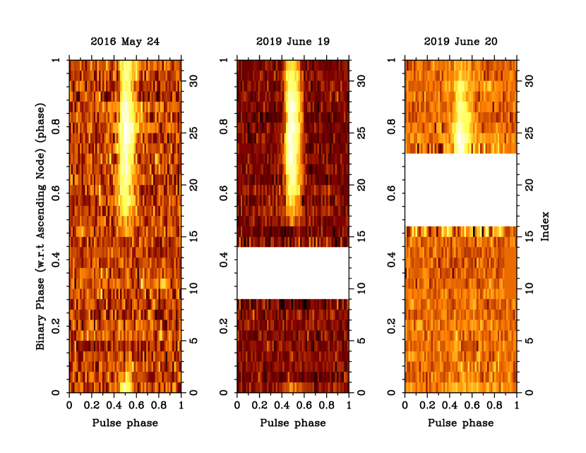
Figure 2: Colour map of the pulse amplitude vs. spin and orbital phase (horizontal and vertical axis, respectively) for the 1.4 GHz 2016 May 24 (left panel), 2019 June 19 (mid panel) and 2019 June 20 (right panel) observations, which have the largest orbital phase coverage. In the mid and right panels the horizontal white band marks the orbital phase ranges that have not been covered by the observations. In all panels the scale on the left-hand side vertical axis is the orbital phase and that on the right one is the sub-integration number (Index). The occurrence of a signal eclipse is apparent in all three panels, although the orbital phase range (0.1–0.5) defined by the eclipse start and end is uniformly covered only by the first observation.

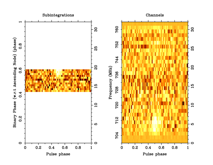
Figure 3: Colour map of the pulse amplitude vs. spin and orbital phase (left panel), and frequency (right panel) for the 2015 April 12 observation at 0.7 GHz.

The edges of the eclipse do not show any evidence of pulse delay or broadening. Such a relatively sharp disappearance of the signal can be ascribed to either a true occultation by the companion, or the presence of intra-binary gas, either very hot or very cold. Indeed, the orbital phase extent of the eclipse is undoubtedly at odds with the occultation scenario, since this would require that the pulsar is in a nearly surface-grazing orbit around the star, hence with an orbital period much shorter than observed. Moreover, a search for signal eclipses in the $\gamma-$ray data (Paper I) ruled out eclipses lasting longer than 0.1% of an orbital period (about 20 seconds), suggesting that the star does not ever properly occult the pulsar. The intra-binary gas scenario is instead an explanation that also confirms the RB classification for PSR J2039$-$5617, initially proposed on the basis of optical observations (Salvetti et al. 2015; Strader et al. 2019).

The occurrence of signal eclipses at 3.1 GHz can neither be confirmed nor ruled out. Figure 4 displays the signal amplitude as a function of pulse and orbital phases for the 2016 May 8 full orbit observation. The right-hand panel shows the pulse profiles of each sub-integration from the left-hand panel. For each profile in the right panel the mean orbital phase (left-hand side scale) and S/N (right-hand side scale) is also reported. It is not clear, from visual inspection of the left panel, whether or not the pulse remains detectable around superior conjunction. Moreover, no single pulse profile appears to feature the typical pure noise profile, and for those profiles where the pulsations seem less evident the corresponding S/N is not low enough to firmly rule out the detection of a pulse. If eclipses do indeed also occur at 3.1 Ghz, the current data suggests that they would occur around the same orbital phase as at 1.4 GHz but their duration would be much shorter. This behaviour would be in line with what is observed in other eclipsing radio pulsars, e.g. PSR J1748-2446A in the globular cluster Terzan 5 (Rasio et al. 1991). Therefore, the physical origin of possible signal eclipses at 3.1 GHz is most likely the same as at 1.4 GHz: the non-detection of pulses is due to a signal absorption which is less effective as the frequency increases, since the optical depth inversely scales with the frequency, in some cases $\propto\nu^{-0.4}$ (see, e.g., Broderick et al. 2016; Polzin et al. 2018).

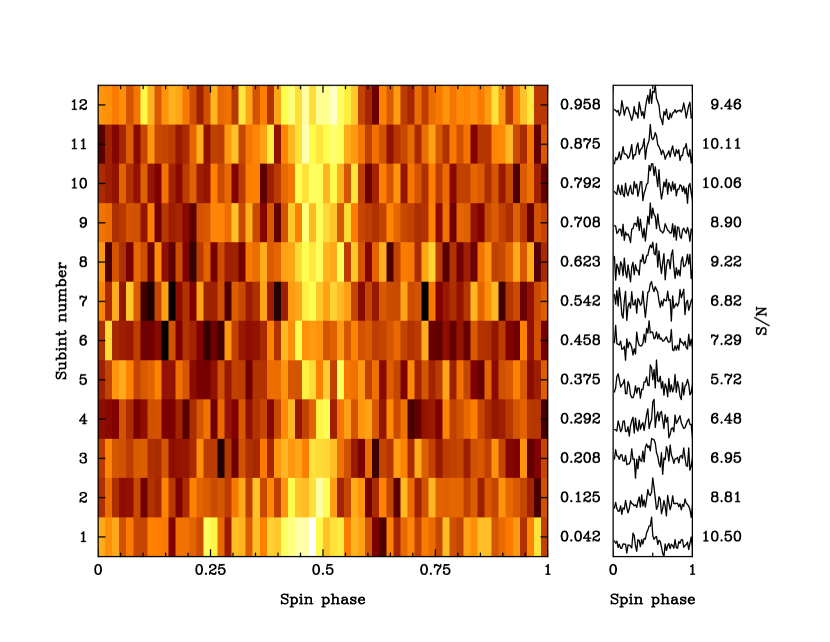
Figure 4: Left panel: colour map of the pulse amplitude vs. spin and orbital phase (horizontal and vertical axis, respectively) for the 2016 May 8 3.1 GHz full-orbit observation. Right panel: stack plot of the pulse profile of each sub-integration in the left panel, whose S/N are reported on the right. The scale between the two panels indicates, for both panels, the mean orbital phase of each sub-integration/profile. The relatively high S/N level across all profiles seems to suggest that the radio signal is not eclipsed across the entire 3.1 GHz (see discussion in §3.3.1).

The phenomenology described above also allows us to shed some light on the observations where pulses have not been detected. The archival observation on 2015 April 9 and our own on 2016 August 19 were carried out when the pulsar was in an orbital phase range where the signal is not detected in other observations. The non-detections of PSR J2039$-$5617 in the 2015 April 12 and 2016 July 6 3.1 GHz data are, instead, not related to an unfavourable orbital phase, since in the 2015 data PSR J2039$-$5617 has been detected at 0.7 GHz and in the 2016 one the observation has been carried out around inferior conjunction. In the case of the 2015 data, this is most likely the effect of interstellar scintillation (§3.3.2), a phenomenon that can occur at such a high frequency (see, e.g., Lewandowski et al. 2011, who studied the scintillation parameters of the pulsar PSR B0329+54 at 4.8 GHz). In the case of the 2016 data, scintillation can be a possible explanation too. Another possible explanation invokes a time-variable distribution of the intra-binary plasma, whose effects on the pulsar signal consequently change with time. If this were the case, the degree of variability of the intra-binary gas structure would have to be extremely high, requiring it to change from a situation where the signal is unaffected for about half orbit at 1.4 Ghz, to another one where it embeds the whole binary system with a density high enough to completely absorb the pulsar signal at 3.1 GHz. Such dramatic changes have indeed been observed in the binary RB PSR J1740-5340A (D’Amico et al. 2001), where delays of the signal at 1.4 GHz are observed at all orbital phases, and the phases at which they occur change substantially from one orbit to another. The companion in that system has a mass of $M_{\rm C}=0.22-0.32\,M_{\odot}$ (Ferraro et al. 2003). The behaviour of the signal delays in this system are explained with a high degree of instability of the intra-binary gas structure, such that it can sometimes embed the whole binary, but at other times leaves more than half of the orbit unocculted. PSR J2039$-$5617 has a similar mass companion in a much tighter orbit. It is therefore possible that when the intra-binary gas is at its maximum size the entire orbit may lie within the innermost region where the gas density is high enough to completely absorb the pulsar signal at 3.1 GHz. We recall (see Table 2) that the orbital phase range covered by the 2016 July 6 observation begins at $\phi_{\rm orb}=0.76$, i.e. at inferior conjunction.

Another explanation for the non-detection on 2016 July 6 might be that of a turn-off of the radio emission, following a transition from a rotation-powered to an accretion-powered state, implying that PSR J2039$-$5617 is a transitional RB. Such scenario would require the occurrence of two transitions between 2016 May 24 and 2016 September 9, two epochs when PSR J2039$-$5617 has been detected as a radio pulsar, and the observation of evidence for the presence of an accretion disk. No long-term change in the $\gamma$-ray flux is seen in the 12-year monitoring of the source by the Fermi-LAT (Paper I), which one would expect to see from a RB undergoing a transition (e.g. Torres et al. 2017, Papitto & De Martino 2020). Moreover, the analysis of optical data taken between 2016 April 30 and September 11 at 37 different epochs by Strader et al. (2019) rules out this scenario. No evidence of optical emission lines due to the presence of an accretion disk has been found in any of the mentioned observation, thus implying that 4FGL J2039.5$-$5617 remained in its radio pulsar state between 2016 April and September.

3.3.2 Pulse brightness vs frequency

Figure 5 displays a colour map of pulse amplitude against pulse phase and observing frequency for 1.4 GHz observations where pulses have been detected. The right panel of figure 3 displays the same plot for the 0.7 GHz data taken on 2015 April 12. As can be seen, the pulse brightness is not uniform across the whole band, but peaks in certain frequency ranges, which vary at random in the four observations at 1.4 GHz. Similarly, the pulse brightness also varies in a random way across the observations. Behaviour of this kind is typical of interstellar scintillation, which is to be expected at these frequencies for a dispersion measure of a few tens of pc cm^-3. The observed flux variations are consistent with the values for the decorrelation bandwidths, $\Delta\nu_{\rm s}=8.8_{-2.9}^{+5.6}$ MHz at 1.4 GHz and $\Delta\nu_{\rm s}=2.1_{-0.7}^{+1.3}$ MHz at 0.7 GHz, and the scintillation times, $\Delta t_{\rm s}=535_{-53}^{+83}$ s at 1.4 GHz and $\Delta t_{\rm s}=390_{-39}^{+61}$ s at 0.7 GHz, predicted by the NE2001 model for the Galactic electron distribution along the LOS to PSR J2039$-$5617 at the measured DM.

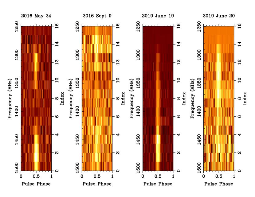
Figure 5: Colour map of the pulse amplitude as a function of the pulse phase and frequency channel for all the 1.4 GHz observations where pulses have been detected, left to right: 2016 May 24, 2016 September 9, 2019 June 19 and 2019 June 20. In all panels, the scale on the right-hand side vertical axis is the frequency channel. The pulse discontinuity at random frequencies is apparent across all the observations and is caused by interstellar scintillation (see discussion in §3.3.2).

The left-hand panel of Figure 6 displays the same plot as in Figure 5 but for the 3.1 GHz full-orbit observation. As in the 1.4 GHz data, the pulse brightness is not uniform across the entire frequency range. The pulse is brighter at lower frequencies (2600–2800 MHz) although it is still clearly detectable at higher frequencies (2900–3400 MHz). The NE2001 model predicts a decorrelation bandwidth at this frequency of $\Delta\nu_{\rm s}=3.8_{-1.3}^{+2.4}$ GHz, which implies the visibility of pulses along a 1 GHz frequency band at 3.1 GHz. The two right panels in Figure 6 display the integrated profiles for each half of the band, and confirm that the pulsed emission is detectable along the entire 3.1 GHz.

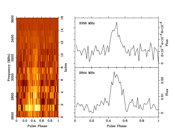
Figure 6: Left: colour map of the pulse amplitude as a function of the pulse phase and frequency for the 2016 May 8 3.1 GHz observation. Right: Pulse profile at two different frequencies close to the extremes of the 3.1 GHz where pulsations are detectable.

3.4 Pulsar Flux

By using the radiometer equation we obtained a preliminary estimate of the radio flux density of PSR J2039$-$5617. To this aim, we considered all observations where pulses have been detected, thus obtaining the flux density at three frequencies. For each observation, we considered those sub-integrations and channels only where pulses were clearly visible. We performed this selection by using the interactive routine pazi. We did our selection separately for sub-integrations and channels, and we adopted an inverse approach: we removed channels/sub-integrations in which the pulse was bright and proceeded until the resulting integrated profile showed no evidence of pulsation. Integration times and bandwidths where the data meet the above requirement are listed in Table 2. For those observations where the signal was detected in separate frequency sub-bands, the reported bandwidth is the sum of the single signal bandwidths in each archive. In the considered 3.1 GHz archive, we did not discard any sub-integration (§ 3.3.1) nor any channel (§ 3.3.2). The resulting archives have been processed with the routine pdmp to obtain the pulses’ S/N, whose values are reported in Table 2. As discussed in § 3.2, the pulse equivalent width, i.e. the width of an equal height and area rectangle, is $W_{\rm eq}=0.1$ in pulse phase at all considered frequencies.

The radiometer equation also requires the values for the system temperature $T_{\rm sys}$ and gain $G$ for each receiver. The Parkes telescope documentation reports a $T_{\rm sys}$ of 40 and 35 K for the 40cm (0.7 Ghz) and the 10cm (3.1 GHz) feed, respectively, of the 10$-$40 receiver, and a $T_{\rm sys}$ of 28 K for the Multibeam receiver. The reported gain is $G=1.1$ Jy/K for all receivers. The resulting flux densities are reported in Table 2. We strongly invite the reader to consider these values, and their implications, with due care, since is not known how they are affected by interstellar scintillation (§ 3.3.2).

4 Discussion

4.1 Modelling of radio and $\gamma$-ray light curves

In Paper I, the pulsar’s orbital parameters and the companion star’s radial velocity amplitude (measured by Strader et al.  2019), were used to constrain the mass of PSR J2039$-$5617, yielding the constraint that $M_{\mathrm{psr}}\sin^{3}i=1.04\pm 0.05\,M_{\odot}$ for an unknown orbital inclination angle $i$. By fitting models for the companion star to the optical light curves (LCs), the orbital inclination was estimated to be $61\degr<i<78\degr$, which corresponds to a pulsar mass range of $1.1,M_{\odot}<M_{\mathrm{psr}}<1.6\,M_{\odot}$.

The detection of radio pulsations from PSR  J2039$-$5617 (alongside the $\gamma$-ray pulsations) allows for an additional, independent method by which to determine the orbital inclination: joint fitting of the phase-matched radio and $\gamma$-ray LCs. Under the assumption that the pulsar was spun-up to its current spin period through the accretion of stellar material stripped from the companion star, the spin axis of the pulsar will simultaneously have been aligned with the orbital axis of the binary system. Hence, the orbital inclination of the binary system should be equal to the observer angle $\zeta$ associated with the pulsar (the angle between the observer’s line of sight and the pulsar’s spin axis), which can be estimated through joint fits to the pulsar’s radio and $\gamma$-ray LCs.

To align the radio and $\gamma$-ray pulse profiles in phase, we took the 2019 June 19 radio data, which had the highest signal-to-noise ratio, and folded using the $\gamma$-ray ephemeris. As mentioned in Section 3.1, there was still a small linear trend in the pulse phase. We therefore refit the orbital phase to account for this, finding a small offset consistent with the uncertainty from the $\gamma$-ray ephemeris. This offset leads to a negligible phase shift of less than 0.4% of a rotation, around 12% of the width of the phase bins adopted for the $\gamma$-ray pulse profile. Along with the best-fitting DM, the epoch, observing location and observing frequency defining the fiducial phase zero (the tempo2 parameters TZRMJD, TZRSITE and TZRFRQ, respectively; Hobbs et al. 2006) were used to phase-align the $\gamma$-ray pulse profile to the radio one.

To constrain the value of $\zeta$ for PSR  J2039$-$5617, two joint fits to the radio and $\gamma$-ray LCs were conducted. These fits yielded not only constraints on $\zeta$, but also on the pulsar’s magnetic inclination angle $\alpha$ (the angle between the pulsar’s magnetic field and spin axes). The geometric outer gap model (OG; Venter et al.  2009), which is a representation of the physical OG model (Cheng et al.  1986a), was used to model the $\gamma$-ray emission for the first of these fits, while the geometric two-pole caustic model (TPC; Dyks and Rudak, 2003), which is a representation of the slot gap physical model (Arons, 1983; Muslimov and Harding, 2003; Muslimov and Harding, 2004), was used for the second. For both fits, an empirical single-altitude hollow cone geometric model (henceforth simply “Cone”; Story et al.  2007) was used for the radio emission. The observed radio and $\gamma$-ray LCs were binned with $n_{\mathrm{r}}=64$ and $n_{\gamma}=30$ equally-spaced phase bins, respectively, and model LCs binned to match.

We note that the geometric OG and TPC models are based on the retarded vacuum magnetic field structure (Deutsch 1955), while newer kinetic (particle-in-cell) models calculate the magnetic field structure for different assumptions on the plasma density, and therefore cover the entire spectrum from vacuum to force-free (plasma-filled) magnetospheres (e.g., Cerutti et al. 2016, Kalapotharakos et al. 2018, Philippov & Spitkovsky 2018). In the former group of models, $\gamma$-ray emission occurs in regions interior to the light cylinder (where the rotation speed equals that of light in vacuum), while in the latter group, particle acceleration, and therefore $\gamma$-ray emission, is ever more constrained to the equatorial current sheet region close to and beyond the light cylinder as the particle density increases. While the latter group of models may be more realistic, we opt to use the OG and TPC models in this paper for a number of reasons. First, the newer models are computationally very expensive, and are typically only solved over a course grid in $\alpha$ and $\zeta$ (and spin-down luminosity). In contrast, the results presented in this paper for the OG and TPC models benefit from a $1\degr$-resolution in these angles. Second, these newer models make a number of assumptions, and their physics is still being constrained by data. For example, they invoke scaled-down magnetic fields to make their calculation feasible, as well as a variety of assumptions regarding particle injection rates, and rely on an approximate treatment of the pair production process. Their use may therefore not necessarily lead to statistically improved LC fits (compared to those that result when the OG and TPC models are used), both in the $\gamma$-ray–only and joint-fitting contexts. On the contrary, for some of the newer models, the LC shapes they produce do not seem to be representative of those observed from the $\gamma$-ray pulsar population. Third, the newer models typically focus on the $\gamma$-ray band and do not take the constraints yielded by the radio models into account. This means that there is no clear consensus on how the assumptions and simplifications these models rely on affect the predicted radio emission. In contrast, our joint fits are performed within a single, unified framework, wherein the radio and $\gamma$-ray emission occur within the same magnetic field structure. This is especially relevant when performing joint LC fits, since it is not only the $\gamma$-ray–band goodness of fit that determines which parameter combination is preferred, but also, equally, the radio-band goodness of fit. Lastly, it is interesting to note that the sky maps (the distribution of radiation vs. $\zeta$ and observer phase) are broadly similar for these two groups of models, despite the differences in the mechanisms by which the caustics (which lead to LC peaks as a fixed observer cuts through them) are formed; compare Fig. $15-17$ of Kalapotharakos et al. (2018) and Fig. 8 of Philippov & Spitkovsky (2018) with Fig. $16-17$ of Venter et al. (2009) as well as Fig. 10 in this paper. This confirms the foresight by Venter & Harding (2014), based on prior LC fitting, that newer models should exhibit hybrid behaviour between OG and TPC models. Comparing the $\gamma$-ray LC for PSR J2039$-$5617 presented here to the published atlas of Kalapotharakos et al. (2018), we roughly obtain $\alpha\sim 45\degr$ and $\zeta\sim 75\degr$ (for a given particle injection rate and spin-down power), which is similar, given all the uncertainties, to the values we find and will discuss later in this section for the OG and TPC models. Notably, the model atlases associated with the other newer models do not contain LCs with shapes that would fit that observed for PSR J2039$-$5617, given the different model assumptions that lead to different emissivity distributions.

The parameter space of the OG and TPC models, ${\alpha,\zeta\in(0\degr,90\degr)}$, was explored at $1\degr$ resolution, yielding 8,100 candidate pairs of phase-matched radio and $\gamma$-ray model LCs for each fit. Since it is unknown a priori (at least solely based on the observed LCs) when (i.e., where in phase) the pulsar’s magnetic field axis is pointing in the observer’s direction, an additional phase shift parameter $\phi_{\mu}$ was added and explored at a resolution equal to twice the radio LC bin width of $(1/64)$th of a rotation.

With this additional parameter implemented, each fit comprised a total of 259,200 model LC pairs. As a last step, the amplitudes $A_{\mathrm{r}}$ and $A_{\gamma}$ of each of the radio and $\gamma$-ray LCs above the relevant background levels were independently adjusted so as to maximize the level of goodness of fit. In total, then, each pair of model LCs in both fits is associated with five model parameters: $\alpha$, $\zeta$, $\phi_{\mu}$, $A_{\mathrm{r}}$, and $A_{\gamma}$. Since the radio and $\gamma$-ray LCs have 64 and 30 bins, the joint fits therefore have $\nu_{\mathrm{c}}=(64+30)-5=89$ degrees of freedom, and the single-band–only fits have $\nu_{\mathrm{r}}=64-4=60$ and $\nu_{\gamma}=30-4=26$ degrees of freedom.

The joint dual-band goodness of fit of each model LC pair $M_{\mathrm{c}}=(M_{\mathrm{r}},M_{\gamma})$ was characterized using the scaled-flux standardized (SFS) $\Psi^{2}_{\Phi,\mathrm{c}}$ goodness-of-fit statistic. Given an observed pair of phase-matched radio and $\gamma$-ray LCs, with associated background levels $b_{\mathrm{r}}$ and $b_{\gamma}$, respectively, this statistic is defined as (Seyffert et al. 2016, Seyffert et al. 2020)

$$\Psi^{2}_{\Phi,\mathrm{c}}(M_{\mathrm{c}})=1-\frac{1}{2}\left(\frac{\chi^{2}_{\mathrm{r}}(M_{\mathrm{r}})}{\Phi^{2}_{\mathrm{r}}}+\frac{\chi^{2}_{\gamma}(M_{\gamma})}{\Phi^{2}_{\gamma}}\right),$$ (1)

where $\chi^{2}_{\mathrm{r}}$ and $\chi^{2}_{\gamma}$ are the $\chi^{2}$ statistics appropriate for the radio and $\gamma$-ray components of the joint fit, and ${\Phi^{2}_{\mathrm{r}}=\chi^{2}_{\mathrm{r}}(B_{\mathrm{r}})}$ and ${\Phi^{2}_{\gamma}=\chi^{2}_{\gamma}(B_{\gamma})}$ are the squared radio and $\gamma$-ray scaled fluxes, where ${B_{\mathrm{r}}=(B_{\mathrm{r},i}=b_{\mathrm{r}})_{n_{\mathrm{r}}}}$ and ${B_{\gamma}=(B_{\gamma,i}=b_{\gamma})_{n_{\gamma}}}$ are the constant radio and $\gamma$-ray background-only LCs implied by $b_{\mathrm{r}}$ and $b_{\gamma}$. The scaled fluxes $\Phi_{\mathrm{r}}$ and $\Phi_{\gamma}$ (both squared in Eq. [1]) measure the total, pulsar-associated flux contained in the observed radio and $\gamma$-ray LCs, and are leveraged in Eq. (1) to effectively express the component single-band–only deviations ($\chi^{2}_{\mathrm{r}}$ and $\chi^{2}_{\gamma}$) in units compatible under addition.

The SFS assigns a goodness-of-fit value of 1 to a ‘perfect’ fit to the data (for which $\chi^{2}_{\mathrm{r}}=\chi^{2}_{\gamma}=0$), and a goodness-of-fit value of 0 to a fit that is equivalent to assuming the background-only LC pair $B_{\mathrm{c}}=(B_{\mathrm{r}},B_{\gamma})$ (for which $\chi^{2}_{\mathrm{r}}=\Phi^{2}_{\mathrm{r}}$ and $\chi^{2}_{\gamma}=\Phi^{2}_{\gamma}$). A negative value for $\Psi^{2}_{\Phi,\mathrm{c}}$ therefore indicates that $M_{\mathrm{c}}$ is a worse fit than $B_{\mathrm{c}}$. The model LC pair $M^{\mathrm{sfs}}_{\mathrm{c}}$ for which $\Psi^{2}_{\Phi,\mathrm{c}}(M^{\mathrm{sfs}}_{\mathrm{c}})=\Psi^{2}_{\Phi,\mathrm{c,max}}$, is the model’s best fit, and the parameter combination associated with it constitutes an estimate of the pulsar parameters.

Since $\Psi^{2}_{\Phi,\mathrm{c,max}}$ is not simply $\chi^{2}$-distributed, constraints on the parameter estimate due to uncertainties in the LC data are obtained using a Monte Carlo algorithm. In analogue to the procedure outlined in Avni (1976) for the $\chi^{2}$ statistic, the goal of this Monte Carlo algorithm is to numerically characterize, via a series of perturbations of the observed LC within its stated flux errors, the distribution of $\Delta\Psi^{2}_{\Phi,\mathrm{c}}=\Psi^{2}_{\Phi,\mathrm{c}}(M^{\mathrm{sfs}}_{\mathrm{c},k})-\Psi^{2}_{\Phi,\mathrm{c}}(M^{\mathrm{sfs}}_{\mathrm{c}})\geq 0$, where $M^{\mathrm{sfs}}_{\mathrm{c},k}$ is the model’s best fit in the $k$th iteration (which may or may not be $M^{\mathrm{sfs}}_{\mathrm{c}}$), and both $\Psi^{2}_{\Phi,\mathrm{c}}$ values are calculated with respect to the $k$th-iteration (i.e., perturbed) observed LCs. Specifically, the goal of the algorithm is to find an estimate $\delta_{3\sigma}$ for this distribution’s $3\sigma$ confidence limit. In the interest of reliability, the algorithm terminates iteration based on a convergence criterion for $\delta_{3\sigma}$ (which is calculated at the end of each iteration): At $200$ iteration intervals (starting from the $400$th iteration), the standard deviation in $\delta_{3\sigma}$ across the preceding $200$ iterations is calculated; if this deviation is less than $5\%$ of $\delta_{3\sigma}$ itself for two consecutive such intervals, iteration is halted. The final value for $\delta_{3\sigma}$ is then converted into an acceptance contour in parameter space by identifying all the LC pairs for which $\Psi^{2}_{\Phi,\mathrm{c}}\geq\Psi^{2}_{\Phi,\mathrm{c,max}}-\delta_{3\sigma}$. The extent of this contour for each parameter then translates into the desired constraint on that parameter.

The SFS statistic, as compared to the corresponding Pearson’s $\chi^{2}$ statistic ${\chi^{2}_{\mathrm{c}}(M_{\mathrm{c}})=\chi^{2}_{\mathrm{r}}(M_{\mathrm{r}})+\chi^{2}_{\gamma}(M_{\gamma})}$, is better suited to joint fits where the single-band–only best fits associated with the component single-band models correspond to contradictory estimates for the shared model parameters (in this case $\alpha$, $\zeta$, and $\phi_{\mu}$), i.e., where single-band LC fitting yields best-fit parameter estimates that are non-colocated in parameter space. Joint fits where such non-colocation is present are susceptible to single-band (typically radio) dominance, particularly in cases where the relative errors in one band are much smaller than those in the other. For example, if the single-band parameter estimates are non-colocated and the relative errors are much smaller for the radio LC than for the $\gamma$-ray LC, the joint fit will be radio dominated, with the best-fit LC pair typically comprised of a good fit to the radio data and a very bad fit to the $\gamma$-ray data.

Seyffert et al. (2016) demonstrate that the SFS statistic effectively eliminates single-band dominance in joint fits, and that the best-fit parameter estimates obtained using the SFS statistic converge to those obtained using $\chi^{2}_{\mathrm{c}}$ as the respective single-band parameter estimates become more colocated and the error disparity dissipates. In essence, the SFS statistic yields a compromise solution that typically reproduces the broad LC structure in both bands, despite any error disparity that might exist.

Table 3: Single-band–only goodness-of-fit values and parameter estimates for PSR J2039$-$5617. Higher values for $\chi^{2}_{\nu}$ indicate decreased goodness of fit.

Fit	$\alpha$	$\zeta$	$\phi_{\mu}$	$\beta$	$\chi^{2}_{\nu}$
	($\degr$)	($\degr$)		($\degr$)
Cone	$58^{+3}_{-2}$	$20^{+3}_{-1}$	$-0.13$	$-38^{+1}_{-1}$	$1.68$
OG	$71^{+2}_{-2}$	$29^{+3}_{-2}$	$-0.09$	$-42^{+5}_{-4}$	$6.10$
TPC	$53^{+10}_{-5}$	$54^{+4}_{-17}$	$-0.09$	$-1$$1^{+9}_{-25}$	$5.74$

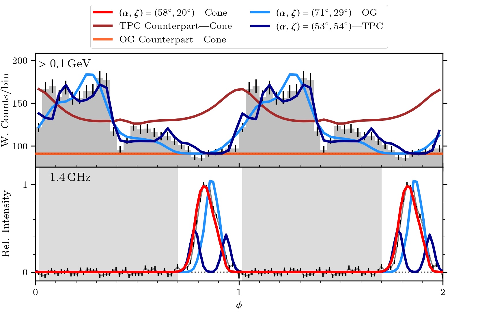
Figure 7: The radio- and $\gamma$-ray–only best-fit LCs for the Cone (red; bottom panel), OG (light blue; top panel), and TPC (dark blue; top panel) models, along with their respective $\gamma$-ray and radio counterparts. The observed radio (bottom panel) and $\gamma$-ray (top panel) LCs (both gray with black error bars) are those observed at 1.4 GHz and at $>0.1$ GeV, respectively. The uniform radio LC error is taken to be the standard deviation of the intensities in the off-peak region (the gray bands).

Table 3 lists the single-band–only parameter estimates, obtained by minimizing $\chi^{2}$ (or, equivalently $\chi^{2}_{\nu}=\chi^{2}/\nu$; the reduced $\chi^{2}$ statistic), which are indeed non-colocated in the models’ shared parameter space (when comparing the radio-only estimate to each of the $\gamma$-ray–only estimates). The radio- and $\gamma$-ray–only best-fit LCs, along with their respective $\gamma$-ray and radio counterparts, are plotted in Figure 7. The radio-only best-fit LC is accompanied by a background-only OG model LC, for which $\chi^{2}_{\nu,\gamma}=\chi^{2}/\nu_{\gamma}=\Phi^{2}_{\gamma}/\nu_{\gamma}=45.00$, and a TPC model LC that is a worse fit than a background-only LC ($\chi^{2}_{\nu,\gamma}=80.40>\Phi^{2}_{\gamma}/\nu_{\gamma}$). The $\gamma$-ray–only best-fit LC for the OG model is accompanied by a comparatively good radio LC ($\chi^{2}_{\nu,\mathrm{r}}=\chi^{2}/\nu_{\mathrm{r}}=54.92\simeq 0.37\times\Phi^{2}_{\mathrm{r}}/\nu_{\mathrm{r}}$), which resembles the shape of the observed radio LC despite the radio peak occurring too late in phase. The best-fit LC for the TPC model is accompanied by a somewhat worse radio fit ($\chi^{2}_{\nu,\mathrm{r}}=113.28\simeq 0.75\times\Phi^{2}_{\mathrm{r}}/\nu_{\mathrm{r}}$), with two radio peaks instead of one. The comparatively better performance of the OG best fit’s counterpart is consistent with the greater agreement between the estimates it and the Cone best fit yield for $\beta=\zeta-\alpha$, the parameter that typically governs peak multiplicity in the Cone model.

4.1.1 The best joint fits

The best-fit LC pair for the OG$+$Cone fit, plotted in green in Figure 8, has a joint goodness-of-fit value of ${\Psi^{2}_{\Phi,\mathrm{c}}=0.883}$ and a reduced $\chi^{2}$ value of ${[\chi^{2}_{\mathrm{c}}]_{\nu}=\chi^{2}_{\mathrm{c}}/\nu_{\mathrm{c}}=6.02}$, as listed in Table 4. The emission maps associated with this LC pair are shown in Figure 9 (top row). The radio-only goodness-of-fit value for this fit is ${\Psi^{2}_{\Phi,\mathrm{r}}=1-\chi^{2}_{\mathrm{r}}/\Phi^{2}_{\mathrm{r}}=0.967}$ (${\chi^{2}_{\nu,\mathrm{r}}=5.01}$), and the $\gamma$-ray–only goodness-of-fit value is ${\Psi^{2}_{\Phi,\gamma}=1-\chi^{2}_{\gamma}/\Phi^{2}_{\gamma}=0.799}$ (${\chi^{2}_{\nu,\gamma}=9.02}$). Notice that, by construction, $\Psi^{2}_{\Phi,\mathrm{c}}=(\Psi^{2}_{\Phi,\mathrm{r}}+\Psi^{2}_{\Phi,\gamma})/2$. These LCs, coupled with the 3$\sigma$ confidence regions shown in white in Figure 10a, correspond to a pulsar parameter estimate of ${(\alpha,\zeta)=((70^{+3}_{-7})\degr,(31^{+12}_{-5})\degr)}$.

Comparing this LC pair to those that correspond to the relevant single-band–only fits puts this joint fit, and the compromise it represents, into its proper context: at the cost of some goodness of fit in the radio band (as compared to the radio-only fit; $\chi^{2}_{\nu,\mathrm{r}}$ increases from $1.68$ to $5.01$), the degree to which the $\gamma$-ray LC is reproduced is increased substantially; from a background-only LC to an LC that is very similar to the $\gamma$-ray–only best-fit LC ($\chi^{2}_{\nu,\gamma}$ decreases from $45.00$ to $9.02$). Or, equivalently (as compared to the $\gamma$-ray only fit), the radio peak’s phase is recovered in the joint fit ($\chi^{2}_{\nu,\mathrm{r}}$ decreases from $54.92$ to $5.01$) at the cost of some goodness of fit in the $\gamma$-ray band ($\chi^{2}_{\nu,\gamma}$ increases from $6.10$ to $9.02$).

Table 4: Joint dual-band goodness-of-fit values and parameter estimates for PSR J2039$-$5617. Higher values for $\Psi^{2}_{\Phi,\mathrm{c}}$, $\Psi^{2}_{\Phi,\mathrm{r}}$, and $\Psi^{2}_{\Phi,\gamma}$ indicate increased goodness of fit, while higher values for $[\chi^{2}_{\mathrm{c}}]_{\nu}$, $\chi^{2}_{\nu,\mathrm{r}}$, and $\chi^{2}_{\nu,\gamma}$ indicate decreased goodness of fit.

Fit	$\alpha$	$\zeta$	$\phi_{\mu}$	$\beta$	$\Psi^{2}_{\Phi,\mathrm{c}}$	$[\chi^{2}_{\mathrm{c}}]_{\nu}$	$\Psi^{2}_{\Phi,\mathrm{r}}$	${\chi^{2}_{\nu,\mathrm{r}}}$	$\Psi^{2}_{\Phi,\gamma}$	${\chi^{2}_{\nu,\gamma}}$
	($\degr$)	($\degr$)		($\degr$)
OG+Cone	$70^{+3}_{-7}$	$31^{+12}_{-5}$	$-0.13$	$-39^{+18}_{-8}$	$0.883$	$6.02$	$0.967$	$5.01$	$0.799$	$9.02$
OG+Cone ($\zeta>50\degr$)	$36^{+5}_{-16}$	$67^{+4}_{-2}$	$-0.13$	$31^{+21}_{-6}$	$0.834$	$11.12$	$0.924$	$11.50$	$0.743$	$11.52$
TPC+Cone (Main)	$61^{+2}_{-1}$	$42^{+2}_{-4}$	$-0.09$	$-19^{+2}_{-5}$	$0.846$	$16.50$	$0.859$	$21.21$	$0.833$	$7.53$
TPC+Cone (Alt.)	$29^{+12}_{-11}$	$67^{+3}_{-6}$	$-0.13$	$38^{+13}_{-16}$	$0.841$	$10.46$	$0.929$	$10.69$	$0.753$	$11.12$

Figure 8: The best-fit LC pairs associated with the OG$+$Cone and TPC$+$Cone dual-band models (solid green and solid brown LCs, respectively). For the TPC$+$Cone model, the best fit included in the alternative contour identified in Figure 10b is also plotted (dashed brown LC). The observed LCs are the same as those in Figure 7.

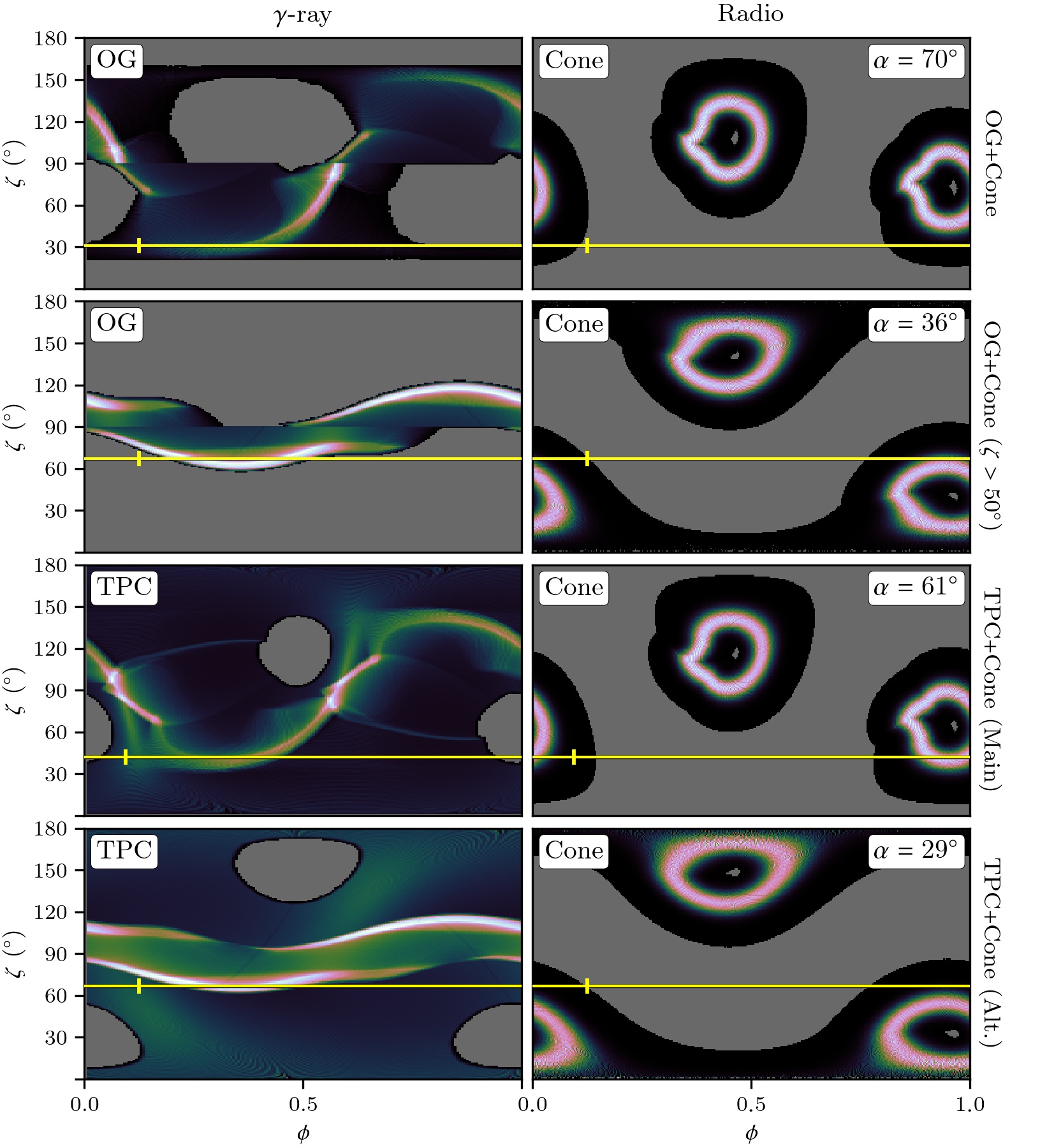
Figure 9: Model radio and $\gamma$-ray emission maps (relative intensity as function of rotational phase $\phi$ and observer angle $\zeta$) for the four joint fits reported in Table 4. The grey regions indicate where the models predict no pulsar-associated emission, i.e., where only background emission will be observed. Each pair (row) of emission maps is associated with a single pulsar inclination angle $\alpha$, and the LC pairs plotted in Figure 8 are each associated with a constant-$\zeta$ cut through the appropriate pair of emission maps (indicated by the horizontal yellow lines). For each cut, the point in model phase that corresponds to 0 in observational phase is indicated by a small vertical tick mark (also yellow).

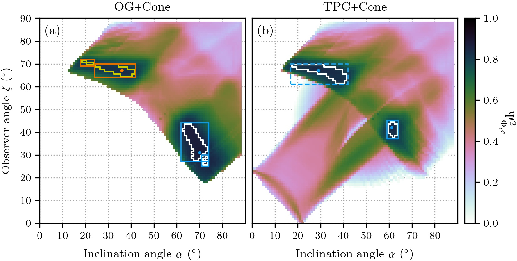
Figure 10: Maps of joint goodness of fit as function of $\alpha$ and $\zeta$ (marginalized over $\phi_{\mu}$) for the OG$+$Cone and TPC$+$Cone dual-band models (panels (a) and (b), respectively) as characterized using $\Psi^{2}_{\Phi,\mathrm{c}}$. Only model LC pairs for which $\Psi^{2}_{\Phi,\mathrm{c}}>0$ and where both wavebands predict pulsar-associated flux, are plotted. In both panels, the white contour demarcates the Monte Carlo–derived $3\sigma$ confidence region(s), and each region’s best fit is indicated with a blue dot. The smaller region for the OG$+$Cone model is considered an extension of the larger region, while the TPC$+$Cone regions are treated as separate regions. The parameter constraints listed in Table 4 are derived from the blue bounding boxes that enclose the various regions.

The TPC$+$Cone fit yielded a pair of confidence regions in $(\alpha,\zeta)$-space: one for which ${\beta<0\degr}$ (the main fit) and one for which ${\beta>0\degr}$. The solid brown LCs in Figure 8 are the best fit included in the former of these regions (enclosed in a solid blue bounding box in Figure 10b), and correspond to a parameter estimate of ${(\alpha,\zeta)=((61^{+2}_{-1})\degr,(42^{+2}_{-4})\degr)}$. Similarly, the dashed brown LCs in Figure 8 are the best fit included in the latter of these regions (enclosed in a dashed blue bounding box in Figure 10b), and correspond to a parameter estimate of ${(\alpha,\zeta)=((29^{+12}_{-11})\degr,(67^{+3}_{-6})\degr)}$. The emission maps associated with these two fits are shown in the bottom two rows of Figure 9, and the associated goodness-of-fit values are listed in Table 4. The overall best fit for this pair of models (TPC$+$Cone) lies inside the $\beta<0\degr$ contour.

Comparing the OG$+$Cone and TPC$+$Cone best fits again demonstrates the effect single-band best-fit non-colocation has on the goodness of fit for the joint fits. For the single-band only fits, the TPC model outperforms the OG model ($\chi^{2}_{\nu}=5.74$ vs. $6.10$), but for the joint fits the OG$+$Cone model outperforms the TPC$+$Cone model ($\Psi^{2}_{\Phi,\mathrm{c}}=0.883$ vs. $0.846$). Understood in terms of compromise, the greater degree of non-colocation between the TPC and Cone estimates necessitates a more costly compromise than that made in the OG$+$Cone fit.

Since an orbital inclination angle of $i<50\degr$ (and hence $\zeta<50\degr$) implies an unrealistically high pulsar mass of $M_{\mathrm{psr}}>2.4\,M_{\odot}$, a second OG+Cone fit was conducted, wherein only model LC pairs for which $\zeta>50\degr$ were considered. The best-fit LC pair thus yielded, which corresponds to a parameter estimate of ${(\alpha,\zeta)=((36^{+5}_{-16})\degr,(67^{+4}_{-2})\degr)}$, is plotted in orange in Figure 8, and the associated confidence region (again derived using a Monte Carlo algorithm) is shown in yellow in Figure 10a (enclosed in an orange bounding box). The emission maps associated with this fit are shown in the second row of Figure 9, and the associated goodness-of-fit values are listed in Table 4. While this fit is worse than the overall OG$+$Cone best fit, as indicated by the lower associated $\Psi^{2}_{\Phi,\mathrm{c}}$ value, it is still a good fit to the overall structure of the observed LCs since its goodness-of-fit value is (substantially) larger than 0.

From these fits, since $\zeta>50\degr$ from the optical fits, we estimate the observer angle to be $\zeta=(67^{+4}_{-2})\degr$ (from the second OG$+$Cone fit) or $\zeta=(67^{+3}_{-6})\degr$ (from the alternative TPC$+$Cone contour). Again assuming that $\zeta\equiv i$, these estimates correspond to mass ranges of $1.17\,M_{\odot}<M_{\rm psr}<1.46\,M_{\odot}$ and $1.19\,M_{\odot}<M_{\rm psr}<1.63\,M_{\odot}$ for the OG$+$Cone and TPC$+$Cone models, respectively. The orbital inclination and pulsar mass estimates obtained here are qualitatively consistent to those found in Paper I, since a fairly low pulsar mass is preferred in both cases. As noted in Paper I, orbital inclination estimates obtained through optical LC models suffer from potentially large systematic uncertainties, and hence the truly independent estimates obtained here are an important validation.

An interesting question is whether the constraints on $\alpha$ and $\zeta$, as found by multi-band light curve modelling, may have implications for heating of the MSP’s stellar companion. The stellar surface of the companion is thought to be heated via the pulsar wind (Stappers et al. 2001), emission from the intrabinary shock (e.g., Bogdanov et al. 2011, Schroeder and Halpern 2014) or particles ducted from the shock along magnetic field lines toward the surface (Romani and Sanchez 2016, Sanchez and Romani 2017), or directly via the pulsed $\gamma$-ray emission from the pulsar. Pulsed magnetospheric $\gamma$ rays typically comprise only $\sim 10\%$ of the energy budget of MSPs (Abdo et al. 2013). In this case, $\alpha$ and $\zeta$ are important in determining the fraction of $\gamma$ rays intercepted by the companion. The companion subtends an angle of $\sim 2\tan^{-1}(1/5)\approx 22^{\circ}\lesssim\alpha$. Thus, if the $\gamma$ rays are isotropically radiated within the opening angle $\sim\alpha$ and spin and orbital axes are aligned, a fraction of $\sim 5\%$ of the total $\gamma$-ray emission will intercepted by the companion at any given orbital phase. Yet, a minor misalignment of spin and orbital axes, by $\sim 10^{\circ}$, would imply that most of the $\gamma$ rays would miss impacting the companion. On the other hand, the pulsar wind may be energetically dominant when considering heating of the companion. The pulsar wind Poynting flux is also anisotropic, and depends on $\alpha$ (e.g., Tchekhovskoy et al. 2016). Since the X-ray double-peaked light curve phasing suggests a shock orientation concave toward the MSP (Wadiasingh et al. 2017), the energetics is largely determined by the opening angle of the shock, which in turn will depend on $\alpha$ and other factors in pressure balance detailed in Wadiasingh et al. (2018). The efficiency of heating depends on the opacity in the photosphere, its ionization state and consequently the spectrum of the impinging radiation field. X-rays from the shock could be more efficient in heating the companion if the ionization fraction is low/moderate, while $\gamma$ rays could penetrate deeper into the companion atmosphere and affect it hydrostatically (e.g., London et al. 1981, Ruderman et al. 1989). Modelling such irradiated atmospheres is a highly nontrivial problem.

4.2 Pulsar distance

Since its $\gamma$-ray discovery, the 4FGL J2039.5$-$5617 distance has been unknown. Based upon the limits on the hydrogen column density $N_{\rm H}$ derived from the fits to the XMM-Newton spectrum, Salvetti et al. (2015) estimated a distance $d\la 0.9$ kpc, consistent with the limits they derived from a colour-magnitude analysis of the putative MSP companion star ($0.2\la d\la 0.9$ kpc). From the stellar proper motion reported in the NOMAD catalogue (Zacharias et al. 2005), and assuming the median of the MSP transverse velocity distribution, Salvetti et al. (2015) inferred a new tentative distance range, which becomes $0.15\la d\la 2.77$ kpc after accounting for the MSP velocity standard deviation. Repeating the same exercise with the more recent stellar proper motion from the Gaia DR2 catalogue, $\mu_{\alpha}\cos\delta=4.21\pm 0.29$ mas yr^-1 and $\mu_{\delta}=-14.93\pm 0.26$ mas yr^-1 (Gaia Collaboration 2018), implies a slightly narrower distance range $0.28\la d\la 2.54$ kpc. More recently, by modelling the optical light curve of the companion star, but with no a priori knowledge of the system’s mass ratio $q$, Strader et al. (2019) derived a larger distance of $3.4\pm 0.4$ kpc. In Paper I, the modelling of the optical light curve based on newly acquired data and the knowledge of the system mass ratio from the $\gamma$-ray and optical mass functions gives 1.7$\pm$0.1 kpc.

With the detection of radio pulsations, the DM provides another way to estimate the source distance, which, however, depends on the assumed electron density model. The DM of $24.57\pm 0.03$ pc cm^-3 implies a distance $d=1.708\pm 0.004$ kpc using the YMW16 model, where the error is only statistical, which becomes as low as $d=0.9\pm 0.2$ kpc using the NE2001 model. The former value is more consistent with the distance of $2.5^{+3.3}_{-0.9}$ kpc inferred from a preliminary optical parallax measurement ($\sim 2\sigma$) of the PSR J2039$-$5617 companion star given in the Gaia DR2 catalogue, whereas the latter is closer to the estimates based on the X-ray observations and on the colour-magnitude analysis. The factor of two discrepancy between the two DM-based values can be smoothed by a more realistic uncertainty estimate for the distances computed through the YMW16 model, for which only the statistical error on the DM is accounted for, whereas for those computed through the NE2001 model, a nominal 20% systematic uncertainty is taken into account, although a factor of 2 higher uncertainty is conservatively assumed in some cases (e.g., Abdo et al. 2013). To quantify the unknown systematic distance uncertainty from the YMW16 model, we have compared the DM-based distances ($d_{\rm YMW16}$) with the parallactic distances ($d_{\pi}$), assumed as a reference, on a sample of 134 pulsars and computed the fractional difference between the two quantities $(d_{\rm YMW16}-d_{\pi})/d_{\pi}$. To filter out obvious outliers we rejected entries where the absolute value of the fractional difference was larger than 1. We found that the mean of the distribution is 0.12, with a standard deviation of 0.40. Our independent uncertainty estimate is in very good agreement with that obtained by Yao et al. (2017) from an analogous comparison based on a different sample of 189 pulsars with either parallactic or other non DM-based distance measurements. Therefore, we assume a realistic uncertainty of 40% on the YWM16 DM-based distance. Under this assumption, the PSR J2039$-$5617 distance would then be $d=1.7\pm 0.7$ kpc, which would be marginally consistent with that obtained from the NE2001 model. The value obtained in Paper I is larger than what we derived from the DM and the NE2001 model and more consistent with that derived from the YWM16 model. An improved, model-free, measurement of the optical parallax of the PSR J2039$-$5617 companion star in one of the next Gaia releases, with DR3 expected in Fall 2021, would hopefully provide an independent confirmation of the presumedly most likely distance value.

4.3 Origin of the radio eclipses

As discussed in § 3.3.1, the most likely explanation for the radio eclipses at 1.4 GHz is attributed to the presence of intra-binary gas. In the case of hot intra-binary gas, the high temperature would imply a very high degree of ionisation, hence a large density of free electrons that rapidly enhance the frequency-dependent signal dispersion in the medium close to the pulsar surface. This effect is not corrected by the signal de-dispersion (§3.1) though, which is applied at a fixed DM value that only accounts for the free electron density in the interstellar medium (ISM). This hot gas would most likely originate from the diffusion of the external layers of the companion star ablated by the pulsar wind, a phenomenon which occurs in RB systems (Rasio et al. 1991). However, the lack of appreciable delays in the radio signal propagation at 1.4 GHz at the edges of the eclipse (Figure 2) is also compatible with an alternative hypothesis of a relatively low ionisation degree of the intra-binary gas. A sanity check for the cold gas scenario is the investigation of possible variations of the dispersion measure along the orbit.

We considered the three observations at 1.4 Ghz where PSR J2039$-$5617 has been observed for a large portion of the orbit, namely the ones taken on 2016 May 24 and the two from 2019. In the corresponding archives, we summed sub-integrations by groups of six, so that the new ones have sub-integrations of one minute, then split these into separated sub-archives with eight sub-integrations each. In this way we obtained archives that span 8 minutes along the orbit, i.e. 2.4% of the orbit. The corresponding orbital phase was determined from the refined value for the time of ascending node passage for the observation (§ 3.1), and the DM obtained by processing these sub-archives with pdmp. We only included phase bins in which we considered the pulse profile to have been detected by visual inspection of the sub-archive integrated profile. Figure 11 plots the variation of the DM for the three mentioned observations with different colors. Each point represents the difference between the DM value for each orbital phase bin and the value for the corresponding whole observation reported in Table 2. Vertical bars correspond to twice the uncertainty of the DM difference, i.e. the 90% confidence level error. All plotted points except two from the 2019 June 20 observation, where the detected pulses are weakest, are consistent with zero DM variation. The mean value for the absolute DM variation $\langle|\Delta DM|\rangle$ and the relative standard deviation $\sigma_{|\Delta DM|}$ are $\langle|\Delta DM|\rangle=$0.116 pc cm^-3 and $\sigma_{|\Delta DM|}=$0.052 pc cm^-3 in the 2015 May 24 observation, $\langle|\Delta DM|\rangle=$0.072 pc cm^-3 and $\sigma_{|\Delta DM|}=$0.051 pc cm^-3 in the 2019 June 19 observation, and $\langle|\Delta DM|\rangle=$0.24 pc cm^-3 and $\sigma_{|\Delta DM|}=$0.13 pc cm^-3 in the 2019 June 20 observation. These quantities are consistent with zero at the 2$\sigma$ level.

Therefore, we can set a 90% confidence upper limit of $\sim$0.4 pc cm^-3 on the maximum amplitude of any orbital phase dependent variations in the DM of the pulsar signal. On one side, this is in agreement with the hypothesis of the presence of a mostly cold intra-binary gas, but, on the other side, that cannot exclude the occurrence of a low density fully ionised gas. Observations over a larger instantaneous bandwidth are needed to improve the sensitivity to DM variations and possibly constrain the thermodynamical status of the intra-binary gas. In both cases, according to the as yet unconstrained size and density distribution of the intra-binary gas, when the pulsar is close enough to the superior conjunction the radio signal can travel an optically thick path and it is simply absorbed by the intervening medium. If its size were up to a few times the size of the Roche Lobe of the companion star, then the cloud might be large enough to embed the whole system, depending on its exact morphology and on the gas confinement status. In this case, for a high enough gas density, the eclipse of the radio signal might be total, which is not the case.

What is in common between the two scenarios is the apparent sudden transition at the edges of the signal eclipses. The 2019 June 19 observation (Figure 2, mid panel) shows a signal behaviour that is fully consistent with what is seen in the above-mentioned data. This fact is consistent with the picture that requires an intra-binary gas whose structure is not perfectly stable in time, but which provides a high optical depth to the propagating signal.

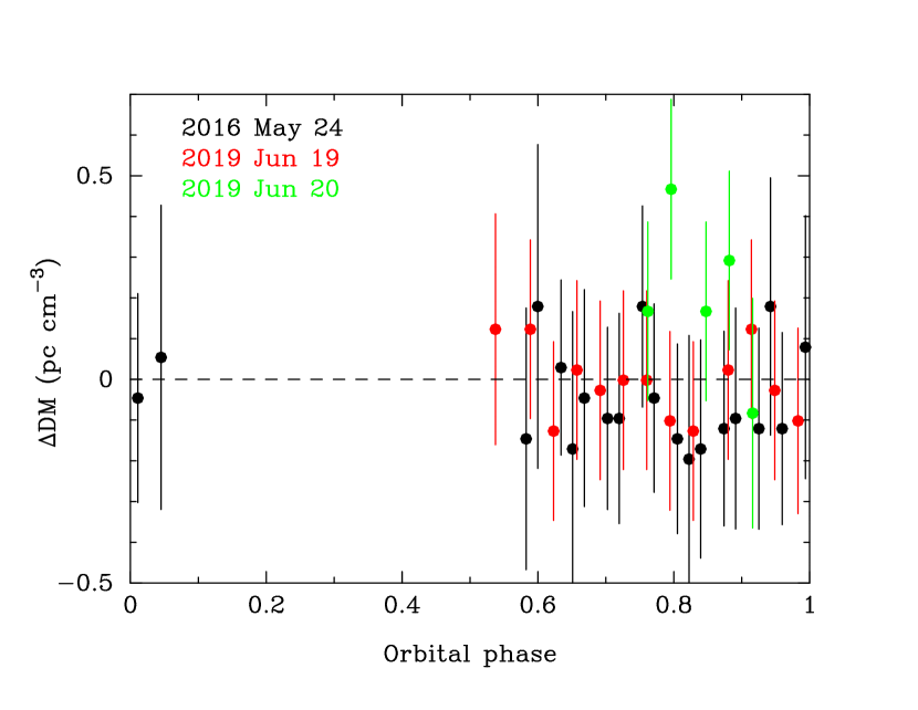
Figure 11: Dispersion measure variations $\Delta$DM versus orbital phase $\phi_{\rm orb}$ for the 2016 May 24 (black), 2019 June 19 (red) and 20 (green) observations. Each data point corresponds to a phase bin of 0.024 orbits (8 minutes), and is the difference between the DM in the phase bin and the DM value of the observation as reported in Table 2. Vertical bars represent twice the uncertainty on $\Delta$DM. Points have only been included if we consider the pulsed to have been detected in a visual inspection of the associated integrated profile.

5 Summary

Through Parkes observations obtained in 2016 we discovered radio pulsations at 0.7, 1.4 and 3.1 GHz from the former RB candidate 4FGL J2039.5$-$5617 following its detection as a $\gamma$-ray pulsar (PSR J2039$-$5617) with spin period $P_{\rm s}\sim 2.6$ ms ( Paper I). At 0.7, 1.4 and 3.1 GHz band, the radio signal consists of a broad single peak. We found clear evidence of eclipses of the radio signal at 1.4 GHz for about 50% of the orbit at pulsar superior conjunction, which proves that PSR J2039$-$5617 features the same radio phenomenology expected for an RB. The origin of the eclipses cannot be unambiguously determined from the available data, which can accommodate absorption of the radio signal by both a cold or a hot intra-binary gas. From our radio observations, we provide the first direct measurement of the dispersion measure (DM = $24.57\pm 0.03$ pc cm^-3), corresponding to a distance of $d=0.9\pm 0.2$ kpc, assuming the NE2001 model, compatible at 1$\sigma$ with that obtained from the YWM16 model, $d=1.7\pm 0.7$ pc cm^-3, after a realistic error treatment. We also measured the pulsar flux density at all the three observing frequencies. A comparison between our 2016 and 2019 1.4 GHz observations of PSR J2039$-$5617 did not unveil any long-term variation in the pulsar radio emission, whereas Neil Gehrels Swift Observatory (hereafter Swift) and Fermi observations showed that the X and $\gamma$-ray fluxes were stable in the time span from June 2017 to May 2018. We will continue our monitoring observations of PSR J2039$-$5617 in both radio and X-rays to look for possible long-term state changes in the source flux and determine whether this is one of the very rare transitional RBs. Finally, we matched the (zero) phases of the radio and $\gamma$-ray pulse profiles finding that the radio pulse leads the main $\gamma$-ray pulse. We also jointly fitted radio and $\gamma$-ray pulses against two geometric models, namely the outer gap (OG) and the two-pole caustic (TPC) ones, and from both models we obtain values for the magnetic field inclination and observer angles, namely $(\alpha,\zeta)=({36^{\circ}}^{+5}_{-16},{67^{\circ}}^{+4}_{-2})$ and $(\alpha,\zeta)=({29^{\circ}}^{+12}_{-11},{67^{\circ}}^{+3}_{-6})$, for the OG and TPC, respectively. Assuming that the pulsar spin axis is aligned to the orbital axis, i.e. $\zeta\equiv i$, the light curve modelling gives an independent measurement of the latter, from which we derive the ranges for the pulsar mass $M_{\rm psr}$ $1.3\,M_{\odot}<M_{\rm psr}<1.5\,M_{\odot}$ and $1.3\,M_{\odot}<M_{\rm psr}<1.6\,M_{\odot}$ for the OG and TPC models, respectively. These ranges are in qualitative agreement to those reported in Paper I.

We conclude by remarking that PSR J2039$-$5617 is now one of a handful of BWs/RBs for which the discovery of an optical/X-ray periodic flux modulation paved the way to the detection of $\gamma$-ray/radio pulsations, after the BW PSR  J1311$-$3430 (Pletsch et al. 2012) and the RB PSR  J2339$-$0533 (Ray et al. 2014). With only a minority of BWs/RBs detected as X-ray pulsars, the search for X-ray pulsations from PSR J2039$-$5617 is now one of the next steps. The case of PSR J2039$-$5617 confirms the validity of the multi-wavelength approach in the identification of BW/RB systems and spurs systematic searches (e.g., Braglia et al. 2020). New BW/RB candidates singled out through the detection of optical/X-ray flux modulations will hopefully be confirmed in the next years once radial velocity measurements provide the values of the orbital parameters to ease blind radio/$\gamma$-ray periodicity searches.

Data availability

The data used in this work are all available in public archives. See references in Section 2.

References

- [] Abdo, A.A. et al., 2013, ApJS, 208, 17
- [] Abdollahi S., et al., 2020, ApJS 247, 33
- [] Acero F., et al., 2015, ApJS 218, 23
- [] Alpar M. A., et. al., 1982, Nature 300, 728
- [] Arons J., 1983, ApJ, 266 215
- [] Arons J. & Tavani M., 1993, ApJ 403, 249
- [] Atwood W. B., et al., 2009, ApJ, 697, 1071
- [] Avni Y., 1976, ApJ 210, 642
- [] Bogdanov, S, Archibald, A.M., Hessels, J.W.T., et al., 2011, ApJ, 742, 97
- [] Braglia C., Mignani R. P., Belfiore A., et al., 2020, MNRAS, 497, Issue 4, 5364
- [] Broderick J. W., et al., 2016, MNRAS 459, Issue 3,2681
- [] Camilo F., et al., 2015, ApJ, 810, 85
- [] Chen H.-L., et al., 2013 ApJ 775, 27
- [] Cheng K. S., Ho C., & Ruderman M. 1986 ApJ 300, 500
- [] Cerutti B., Philippov, A. A., & Spitkovsky, A., 2016, MNRAS, 457, 2401
- [] Clark C., et al., 2020, submitted to MNRAS ( Paper I)
- [] Cordes J. M., & Lazio T. J. W., 2002, arXiv E-prints, arXiv:astro-ph/0207156
- [] D’Amico N., et al., 2001, ApJL 561, L89
- [] Deller A. T., Moldon J., Miller-Jones J. C. A., et al., 2015, ApJ,809, 13
- [] Deutsch, A.J. 1955, Ann. Astrophys., 18, 1
- [] Dyks J., & Rudak B., 2003, ApJ 598, 1201
- [] Ferraro F.R., et al., 2003, ApJl 584, L13
- [] Fruchter, A. S., et al., 1988, Nature 333, 237
- [] Gaia Collaboration, 2016, A&A 595, A1
- [] Gaia Collaboration, 2018, A&A 616, A1
- [] Harding A. K., & Gaisser T. K., 1990, ApJ 358, 561
- [] Hobbs G., et al., 2006, MNRAS, 369, 655
- [] Hobbs G., et al., 2019 arXiv E-prints, arXiv:1911.005656
- [] Hui C.-Y., 2014, J. Astron. Space Sci., 31, 101
- [] Hui C.-Y., et al., 2018, ApJ 864, 30
- [] Hui C.-Y., & Li K.-L, 2019, Galaxies, vol. 7, issue 4, p. 93
- [] Kalapotharakos, C., Brambilla, G., Timokhin, A., Harding, A.K., & Kazanas, D. 2018, ApJ, 857,44
- [] Jankowski F., et al., 2018, MNRAS 473, 4436
- [] Lee J., et al., 2018, ApJ, 864, 23
- [] Lewandowski W., et al., 2011, A&A 534, 66
- [] Linares M., 2019 arXiv E-prints, arXiv:1910.09572
- [] London, R., McCray, R., and Auer, L. H. 1981, ApJ, 243, 970
- [] Manchester R. N., et al., 2005, AJ 129, 1993
- [] Muslimov A.G. & Harding A.K., 2003, ApJ 588, 430
- [] Muslimov A. G. & Harding A. K., 2004 ApJ 606, 1143
- [] Ng C. W., et al., 2018, ApJ 867, 90
- [] Nieder L., et al., 2020, ApJL 902, L46
- [] Papitto A., De Martino D., 2020 arXiv E-prints, arXiv:2010.09060
- [] Petrov L., et al., 2013, MNRAS 432, 1294
- [] Philippov, A.A. & Spitkovsky, A 2018, ApJ, 855, 94
- [] Pletsch H. J., et al., 2012, Science 338, 1314
- [] Polzin E. J., et al., 2018 MNRAS, 476, Issue 2, 1968
- [] Possenti, A., et al., 2003, ApJ 599, Issue 1, 475
- [] Radhakrishnan V. & Srinivasan G., 1982, Current Science 51, 1096
- [] Rasio F. A., Shapiro S. L., & Teukolsky S. A., 1991, A&A 241, L25
- [] Ray P. S., et al., 2013, ApJ, 763, L13
- [] Ray P. S., et al., 2014 American Astronomical Society, AAS Meeting #223
- [] Roberts M. S. E., 2011, in IAU Symp. 291 (Cambridge: Cambridge Univ.Press), 127
- [] Roberts M. S. E., et al., 2014, AN 335, 313
- [] Romani R. W., & Shaw M. S., 2011, ApJL 743, L26
- [] Romani R. W., 2012, ApJ, 754, L25
- [] Romani R. W., 2015, ApJL, 812, L24
- [] Romani, R.W. & Sanchez, N. 2016, ApJ, 828, 7
- [] Ruderman, M., Shaham, J., Tavani, M. & Eichler, D. 1989, ApJ, 343, 292
- [] Salvetti D., et al., 2015, ApJ 814, 88
- [] Sanchez, N. & Romani, R.W. 2017, ApJ, 845, 42
- [] Saz Parkinson P. M., et al., 2016, ApJ 820, 8
- [] Schroeder J., & Halpern J., 2014, ApJ 793, 78
- [] Seyffert A. S., et al., 2016, arXiv E-prints, arXiv:1611.01076
- [] Seyffert A. S., et al., 2020 (in prep.)
- [] Stappers, B.W., van Kerkwijk, M.H., Bell, J.F. & Kulkarni, S.R. 2001, ApJL, 548, L183
- [] Strader J., et al., 2019, ApJ 872, 42
- [] Story S. A., Gonthier P. L., Harding, A. K., 2007 ApJ 671, 713
- [] Tchekhovskoy, A., Spitkovsky, A. & Li, J.G. 2013, MNRAS, 435, L1
- [] Torres D. F., Ji L., Li J., Papitto A., Rea N., de Ona Wilhelmi E., Zhang S., 2017, ApJ, 836, 68
- [] Torres D. F. & Lin J., 2020, in Millisecond Pulsars, Astrophysics and Space Science Library (ASSL) series, Sudip Bhattacharyya, Alessandro Papitto and Dipankar Bhattacharya eds., arXiv:2004.03128
- [] van Kerkwijk M. et al., 2011, ApJ 728, 95
- [] Venter C., Harding A. K., Guillemot L., 2009 ApJ, 707 800
- [] Venter, C. & Harding, A.K. 2014, Astronomische Nachrichten, 335, 268
- [] Wadiasingh, Z., Harding, A.K., Venter, C., et al. 2017, ApJ, 839, 80
- [] Wadiasingh, Z., Venter, C., Harding, A.K., et al., 2018, 869, 120
- [] Yao J. M., et al., 2017, ApJ 835, Issue 1, 29
- [] Zacharias N., et al., 2005, VizieR On-line Data Catalog: I/297