Multiscale simulation of a polymer melt flow
between two coaxial cylinders under nonisothermal conditions

Abstract

We successfully extend a multiscale simulation (MSS) method to nonisothermal well-entangled polymer melt flows between two coaxial cylinders. In the multiscale simulation, the macroscopic flow system is connected to a number of microscopic systems through the velocity gradient tensor, stress tensor and temperature. At the macroscopic level, in addition to the momentum balance equation, we consider the energy balance equation, where heat generation plays an important role not only in the temperature distribution but also in the flow profile. At the microscopic level, a dual slip-link model is employed for well-entangled polymers. To incorporate the temperature effect into the microscopic systems, we used the time-temperature superposition rule for the slip-link model, in which the temperature dependence of the parameters is not known; on the other hand, the way to take into account the temperature effect in the macroscopic equations has been well established. We find that the extended multiscale simulation method is quite effective in revealing the relation between nonisothermal polymeric flows for both steady and transient cases and the microscopic states of polymer chains expressed by primitive paths and slip-links. It is also found that the temperature-dependent reptation-time-based Weissenberg number is a suitable measure for understanding the extent of the polymer chain deformation in the range of the shear rate used in this study.

I Introduction

Polymeric material has found increasingly more applications, such as automobile, fiber, medical and aerospace materials, where it is needed to make polymeric products with high functionalities. To fabricate polymer products, we usually have to address entangled polymer melts. In general, it is difficult to accurately predict processing flow properties because the transport of mass, momentum and energy occur simultaneously in complex flow channel geometries. Moreover, the flow behavior of entangled polymer melts themselves is complex because the macroscopic flow behavior is highly correlated with the microscopic states of polymer chains, such as chain orientations and entanglementsMasubuchi2014 ; Sato2020 .

In this paper, we specifically focus on nonisothermal flows of entangled polymer melts that are frequently seen in the polymer industry. Conventionally, macroscopic approaches are used to simulate the processing flows of entangled polymer melts with temperature changes. In the majority of macroscopic approaches, macroscopic balance equations including the energy balance equation are coupled with a phenomenological constitutive equation with a temperature-dependent relaxation time. One of the phenomenological constitutive equations frequently employed in the polymer industry is the generalized Newtonian fluid constitutive equationBird1987 . This type of constitutive equation, e.g., the Cross modelCross1965 , can reproduce shear-rate-dependence of the viscosity of polymer melts. Furthermore, to address the effect of temperature changes, the generalized Newtonian fluid constitutive equation, including the Cross model, was extended using the Williams-Landel-Ferry (WLF) equationFerry1980 or the Arrhenius law, which is the so-called Cross-WLF model or Cross-Arrhenius model, respectively. In the Cross-WLF model (or the Cross-Arrhenius model), the relaxation time and zero shear viscosity of the polymer melt can be considered to depend on the temperature, which is described by the WLF equation (or the Arrhenius equation). Using the generalized Newtonian fluid constitutive equation, processing flow problems with temperature changes, such as the filling processChiang1991 ; Otmani2011 , flows in an extruderKhalifeh2005 , and flows in a sudden expansion channelZdanski2009 , were investigated. Although the generalized Newtonian constitutive equations with temperature changes can reproduce the shear-rate- and temperature-dependence of the viscosity of polymeric liquids, several properties of polymeric liquids, such as normal stress effects, are not taken into account. More realistically, a viscoelastic constitutive equation with a temperature-dependent relaxation time replaces the generalized Newtonian constitutive equations. Viscoelastic constitutive equations can successfully address normal stress effects or time-dependent effects. By means of these phenomenological constitutive equations, polymer processing flows with temperature changes, such as flows in a polymer melt spinning processDoufas2000 , around a cylinderPeters1997 , and in an abrupt contraction channelKunisch2000 ; Wachs2000 , were extensively investigated. However, there are several problems when employing phenomenological constitutive equations. One of these problems is that phenomenological constitutive equations prohibit one from directly obtaining microscopic insights of polymer chains. Because the microscopic state of polymer chains determines the quality of the resultant polymer product, it has been desired to develop a new simulation technique that can predict not only the macroscopic flow behavior but also the microscopic state of its constituent polymer chains.

For this purpose, an increasing amount of attention has recently been paid to a multiscale simulation (MSS) method that can bridge the gap between the macroscopic flow simulator and a large number of molecular-based polymer dynamics simulators. A pioneering study of multiscale simulations is the Calculation of Non-Newtonian Flow: Finite Elements and Stochastic Simulation Technique (CONNFFESSIT), which was developed by Laso and ÖttingerLaso1993 . In the CONNFFESSIT framework, macroscopic balance equations and a microscopic system consisting of a dumbbell model are successfully combined. As a review on multiscale approaches, the literature by Keunings Keunings2004 will be useful. Based on the CONNFFESSIT, various types of multiscale simulation methods have been proposedHulsen1997 ; Halin1998 ; E2003 ; Yasuda2008 ; Murashima2010 .

Thus far, we have succeeded in applying a multiscale simulation methodMurashima2010 to isothermal flow problems of well-entangled monodispersed polymer melts in various flow geometries such as flows around an infinitely long cylindrical obstacleMurashima2011 ; Murashima2012 , those in a 4:1:4 contraction-expansion channelSato2019a , and those of the polymer melt spinning processSato2017 . In our multiscale simulation for well-entangled polymer melts, a macroscopic flow simulation model for solving the balance equations is combined with a number of microscopic systems described by a slip-link modelDoi2003 . We conducted multiscale simulations of the systems mentioned above under isothermal conditions, but industrial processes are usually performed under nonisothermal conditions. In addition, industrially used polymeric materials are not monodisperse but polydisperse in the molecular weight. These nonisothermal and polydisperse natures of polymeric systems bring various novel flow behaviors and make the flow predictions difficult. The multiscale simulation method used in the present work can be applied to polydisperse systems by simply considering poly-dispersed polymer chains in the slip-link simulator embedded in each Lagrange particle. Hence, the multiscale method would be a potential candidate to deal with such a system. In this work, however, to focus on and to demonstrate how the temperature field affects the macroscopic flow and microscopic state of the polymer chains, we restrict ourselves to a mono-dispersed, but nonisothermal polymeric system. We will tackle the system with polydispersity as future work.

It should be noted that multiscale simulations under a nonisothermal condition using the Kremer-Grest (KG) modelKremer1990 have been performed by Yasuda and Yamamoto, i.e., the so-called synchronized molecular dynamics (SMD)Yasuda2014 . Using SMD, they successfully investigated polymer lubrication problemsYasuda2016 ; Yasuda2019 . However, SMD is currently limited to simple flow problems because this method has, for example, a heavy computational cost. A multiscale simulation technique that employs a more coarse-grained model than the KG model is still desired to consider processing flow problems. Thus, the objective of the present paper is to develop a method to incorporate the effect of the temperature distribution into the multiscale simulation method we have developed thus far. The paper is organized as follows. In Sec. II, we explain the nonisothermal multiscale simulation method, especially how the temperature effect is taken into account in both a macroscopic system and a microscopic system. In Sec. III, we show the results obtained in the application of the extended method to a nonisothermal flow problem between two coaxial cylinders. Finally, in Sec. IV, we draw conclusions regarding the extended multiscale simulation method.

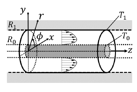
Figure 1: Schematic picture of a coaxial dual-cylinder system

II Model

II.1 Macroscopic System

We consider a polymer melt flow between two infinitely long coaxial cylinders, where the respective radii of the inner and outer cylinders are $R_{0}$ and $R_{1}$ (Fig.1). This type of flow geometry can be seen in manufacturing in polymer products that have a cylindrical cavity along the center line of the cylindrical extrudates, such as a tube, parison, and hollow fiber. The flow problem considered here, however, is somewhat artificial. Because the aim of the present paper is to demonstrate the extensibility of the MSS method, originally developed for iso-thermal flow problems, to nonisothermal flow of well-entangled polymer melts, it is important to make an assessment of the nonisothermal MSS method by choosing a simpler flow geometry. Therefore, we choose this infinitely long coaxial cylinder geometry. To describe this system, we use a cylindrical coordinate system whose $z$-direction is set to the center axis of the coaxial dual-cylinders, whose radial direction is perpendicular to the center axis and whose azimuthal direction ($\phi$-direction) is defined as shown in Fig.1. The flow between the coaxial cylinders is induced by applying a uniform pressure gradient. The temperatures of the inner and outer cylinders are set to $T_{0}$ and $T_{1}$ ($T_{0}\geq T_{1}$), respectively. The viscosity of the polymer melt considered here is high enough such that one can assume a laminar flow. For the sake of the translational symmetry of the system along the $z$-direction, all variables are functions of the radius $r$ and time $t$, and the velocity is expressed as $\bm{v}=v_{z}(r,t)\bm{e}_{z}$, where $\bm{e}_{z}$ is the unit vector along the $z$-axis and the temperature is $T(r,t)$. The equations for $v_{z}$ and $T$ are given by

$$\rho{\partial v_{z}(r,t)\over\partial t}={1\over r}{\partial\over\partial r}\Bigr{(}r\sigma_{rz}(r,t)\Bigr{)}+F_{z}^{(\rm ext)}$$ (1)

$$\rho C_{p}\frac{\partial T(r,t)}{\partial t}=k\frac{1}{r}\frac{\partial}{\partial r}\left(r\frac{\partial T}{\partial r}\right)+\sigma_{rz}\frac{\partial v_{z}}{\partial r}$$ (2)

where $\rho$ is the density of the fluid, $\sigma_{rz}$ is the $rz$-component of the stress coming from the entangled polymer dynamics, and $F_{z}^{(\rm ext)}$ is a constant force density given by a constant pressure gradient along the $z$-direction. In the energy equation (2), $C_{p}$ and $k$ are the specific heat capacity and thermal conductivity of the fluid, respectively. The boundary conditions at the two walls for the velocity and temperature are respectively given as

$$v_{z}(R_{0},t)=0,\quad v_{z}(R_{1},t)=0,$$ (3)

$$T(R_{0},t)=T_{0},\quad T(R_{1},t)=T_{1}.$$ (4)

As the units of length, time and stress, we employ the radius of the outer cylinder $R_{1}$, $\tau_{\text{e}}(T_{\rm ref})$ and $\sigma_{\text{e}}(T_{\rm ref})$, respectively, where $T_{\rm ref}$ denotes a reference temperature. $\tau_{\text{e}}(T_{\rm ref})$ and $\sigma_{\text{e}}(T_{\rm ref})$ are also the units of time and stress for the microscopic model used in the present work, which will be explained later. The velocity and the external force density are scaled by the constructed units $v_{\rm{o}}\equiv R_{1}/\tau_{\rm e}(T_{\rm ref})$ and $F_{\rm{o}}\equiv\sigma_{\rm e}(T_{\rm ref})/R_{1}$, respectively. Generally, the density and the heat capacity of a polymer melt also depend on the temperature, but here, they are treated as constant because their variation with the temperature is considered to be small. In addition, the thermal conductivity $k$ may have a tensorial form $k_{\alpha\beta}$ depending on a local polymer conformation that can be evaluated at the microscopic level in our multiscale simulation. Because the amount of experimental data on the dependence of $k_{\alpha\beta}$ on the polymer conformation is insufficient, the thermal conductivity is also simply assumed to be constant. With the units mentioned above, eqs.(1) and (2) become the following nondimensional expressions:

$${{\sf Re}^{\rm(a)}}\frac{\partial{\tilde{v}}_{z}(\tilde{r},\tilde{t})}{\partial\tilde{t}} = \frac{1}{\tilde{r}}\frac{\partial}{\partial\tilde{r}}\Bigl{(}\tilde{r}\tilde{\sigma}_{rz}(\tilde{r},\tilde{t})\Bigr{)}+{\tilde{F}_{z}}^{\rm{(ext)}}$$ (5)

$${{\sf Pe}^{\rm(a)}}\frac{\partial T(\tilde{r},\tilde{t})}{\partial\tilde{t}} = \frac{1}{\tilde{r}}\frac{\partial}{\partial\tilde{r}}\left(\tilde{r}\frac{\partial T}{\partial\tilde{r}}\right)+{{\sf Br}^{\rm(a)}}\frac{\partial\tilde{v}_{z}}{\partial\tilde{r}}\tilde{\sigma}_{rz}$$ (6)

where the variables with the tilde symbol on top of them are scaled variables. ${\sf Re}^{\rm(a)}$, ${\sf Pe}^{\rm(a)}$ and ${\sf Br}^{\rm(a)}$ are the apparent Reynolds, Péclet and Brinkman numbers, respectively, and are defined as

$${\sf Re}^{\rm(a)}={\rho v_{\rm{o}}R_{1}\over\eta_{\text{e}}(T_{\rm ref})},{\sf Pe}^{\rm(a)}=\frac{v_{\rm{o}}R_{1}}{D_{T}},{\sf Br}^{\rm(a)}=\frac{\sigma_{\rm e}(T_{\rm ref})v_{\rm{o}}R_{1}}{k}~{}~{}~{}~{}$$ (7)

where $\eta_{\text{e}}(T_{\rm ref})=\sigma_{\text{e}}(T_{\rm ref})\tau_{\text{e}}(T_{\rm ref})$ and $D_{T}=k/\rho C_{p}$. The three parameters ${\sf Re}^{\rm(a)}$, ${\sf Pe}^{\rm(a)}$ and ${\sf Br}^{\rm(a)}$ that appear in the macroscopic equations (5) and (6) are determined by the geometry of the system and the material considered here.

II.2 Microscopic Model of Entangled Polymer Chains

As a microscopic model to describe the rheological properties of a well-entangled polymer melt, we employ the dual slip-link model proposed by Doi and TakimotoDoi2003 ; Sato2019b but extend it such that it can describe the dynamics of a well-entangled polymer melt under a time-dependent temperature $T(t)$. Generally, it is not straightforward to incorporate the temperature effect into a coarse-grained polymer model, unlike an atomistic polymer model, because the temperature dependence of parameters used in the coarse-grained model is not clear. It is well known that the time-temperature superposition (TTS) ruleFerry1980 holds for the rheological properties of a homogeneous polymeric liquid, and the temperature effect has been successfully incorporated into a constitutive equation by scaling its parameters based on this time-temperature superposition rule Habla2012 ; Pol2014 ; Zatloukal2016 ; Zhuang2017 ; Gao2019 . The slip-link model is specifically used to describe the rheological properties of a homogeneous well-entangled polymer melt; therefore, the TTS rule can be used inversely to determine the temperature dependence of the parameters used in the coarse-grained model, such as the Rouse and reptation relaxation times, and the temperature dependence of the stress. Namely, the way to incorporate the temperature effect into the model is to use the TTS rule, which means that all the physical quantities related to time and stress must be scaled by shift factors $a_{T}$ and $b_{T}$, respectively. The shift factors $a_{T}$ and $b_{T}$ are given by

$$\log_{10}{a_{T}}=-\frac{C_{1}(T-T_{\rm ref})}{C_{2}+(T-T_{\rm{ref}})},\quad{b_{T}}=\frac{T}{T_{\rm ref}}$$ (8)

where $T_{\rm ref}$ is the reference temperature used in the TTS rule, $C_{1}=8.86$ and $C_{2}=101.6$ K. Here, the expression for the shift factor $a_{T}$ is called the Williams-Landel-Ferry (WLF) equation. Based on this idea, we can extend the slip-link model proposed for an isothermal polymer melt system to a nonisothermal system, where the time unit and the stress unit are scaled by the shift factors $a_{T}$ and $b_{T}$, respectively. By using the extended model, we can apply it to a multiscale simulation of a polymer melt flow with a temperature distribution in a flow channel. The polymer melt considered here is composed of linear polymer chains with a monodisperse molecular weight distribution and with a total number of strands $Z_{0}$ (in other words, with entanglements $Z=Z_{0}+1$) on a single chain in equilibrium.

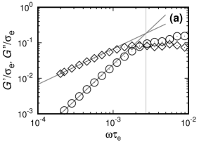
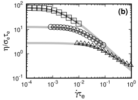
Figure 2: Rheological properties of the polymer melt ($Z_{0}=10$) used in the MSS. (a) linear viscoelasticity at $T=160^{\circ}$C ($\bigcirc$: $G^{\prime}$, $\diamondsuit$: $G^{\prime\prime}$), (b) steady shear viscosity and (c) 1st normal stress difference (open symbol) and 2nd normal stress difference (filled symbol), at $T$=160^∘C ($\square$), 170^∘C ($\bigcirc$), and 180^∘C ($\bigtriangleup$) in (b) and (c). In (b), the top gray line is fitted to the data at 160^∘C ($\square$) using eq.(10), where the estimated fit parameters are $\eta_{0}\left(T_{\rm ref}\right)=78.8$, $n=0.993$ and $C_{3}=4.55$. The remaining two gray lines are drawn by respectively setting the temperature to 170^∘C and 180^∘C in eq.(10), with the estimated parameters unchanged.

In the slip-link model, a polymer chain is expressed by a primitive path and slip-links on the primitive path; thus, the length of a primitive path in equilibrium is $L_{0}=Z_{0}a$, with $a$ being the distance between two consecutive entanglements along a chain in equilibrium. A slip-link represents an entanglement point between two different polymer chains. The number of slip-links $Z$ on a primitive path changes with time $t$. The polymer chain expressed by a primitive path is composed of $Z$ slip-links, $(Z-1)$-strands and two tails. The primitive path length of a polymer chain is given by

$$L=s_{\rm+}+s_{\rm-}+\sum_{j=1}^{Z-1}|{\bm{r}_{j}}|$$ (9)

where $s_{+}$ and $s_{-}$ are the lengths of the head and tail, respectively, and ${\bm{r}}_{j}$ is the relative vector from the position of the $j$-th slip-link to that of the $(j-1)$-th slip-link. For details on the procedure for updating the state of a primitive path and the slip-links of a polymer in a fluid particle, see Appendix I.

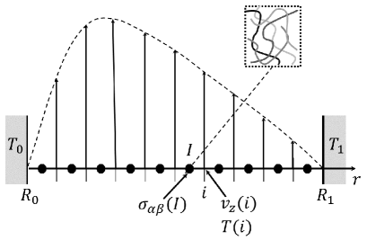
Figure 3: Schematic image of the discretization of the system along the radial direction.

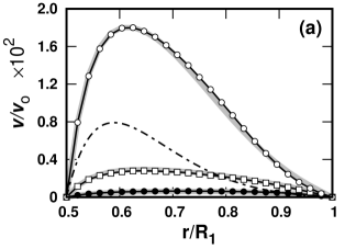
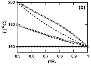
Figure 4: (a) Velocity and (b) temperature profiles along the radial direction at steady states for $T_{0}$ equal to (i) 160^∘C (filled circle), (ii) 180^∘C (open square), and (iii) 200^∘C (open circle). In (a), the dash-dotted line represents condition (iii) but with a Newtonian fluid with zero shear viscosity $\eta_{0}(T)$ $=\eta_{0}(T_{\rm ref})a_{T}b_{T}$ that is equivalent to that of the slip-link model ($Z_{0}=10$). In (b), the dashed line just below each solid line stand for the analytical solution to eq.(6) with ${\sf Br}^{\rm(a)}=0$ and ${\sf Pe}^{\rm(a)}=0$. In (a) and (b), the three thick gray lines underlying the simulations data (filled and open symbols) are obtained from eqs.(5) and (6), with the stress given by the Cross-WLF model of eq.(10), using the estimated fit parameters of Fig.2.

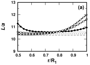
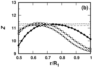
Figure 5: (a) Average length of primitive paths and (b) average number of entanglements on a primitive path as functions of the radius at the steady states for $T_{0}$ equal to (i) 160^∘C (filled circle), (ii) 180^∘C (open square), and (iii) 200^∘C (open circle). The dotted, dashed, and long-dashed lines stand for the data in equilibrium at $T_{0}=$160, 180, and 200^∘C, respectively.

II.3 Bulk Rheological Properties of a Polymer Melt

As the polymer melt in our simulation, we consider a system of monodispersed entangled linear polystyrene (PS). Each of the constituent polymers has ten entangled strands $Z_{0}=10$ (i.e., eleven entanglement points, $Z=11$) in equilibrium, which correspond to a polystyrene with a molecular weight of $1.4\times 10^{5}$. We first investigate linear viscoelastic properties and the bulk steady shear viscosity of the polymer melt, which are used in our multiscale simulations in Sec. III. In Fig.2(a), we show the storage modulus $G^{\prime}$ and loss modulus $G^{\prime\prime}$ evaluated from the stress relaxation modulus $G(t)$ after applying a step shear strain with $\gamma_{0}=0.5$ to the entangled polymer melt at $T=160^{\circ}$C. The reptation time $\tau_{\rm{d}}$ is found to be $366\tau_{\text{e}}$ at $160^{\rm o}$C from the intersection of the two lines (gray lines in Fig.2(a)) fitted to $G^{\prime}$ and $G^{\prime\prime}$ in the terminal relaxation region. Fig.2(b) shows the steady shear viscosities of the previously mentioned polymer melt at three temperatures: 160^∘C, 180^∘C and 200^∘C. As seen from Fig.2(b), the systems exhibit the shear thinning behavior. To analyze the temperature dependent shear thinning behavior, we used the following Cross-WLF model, defined as

$$\eta(\dot{\gamma},T)={\eta_{0}(T_{\rm ref})a_{T}b_{T}\over 1+C_{3}(\eta_{0}(T_{\rm ref})a_{T}|\dot{\gamma}|)^{n}}$$ (10)

where $\eta_{0}(T_{\rm ref})$ is the zero shear viscosity of the polymer melt at $T_{\rm ref}$, $C_{3}$ and the exponent $n$ are fitting parameters. By fitting the data obtained by the slip-link model at $T_{\rm ref}=160^{\circ}$C with the Cross-WLF model (eq.(10)), the parameters are found to be $\eta_{0}\left(T_{\rm ref}\right)=78.8$, $n=0.993$ and $C_{3}=4.55$. In Fig.2(b), the fitted line for $T_{\rm ref}=160^{\circ}$C, together with the corresponding lines for $T=180^{\circ}$C and $T=200^{\circ}$C, evaluated using the same parameter values, are drawn using thick gray lines. One can clearly see that the temperature dependent shear thinning behaviors are captured by the Cross-WLF model.

II.4 Multiscale Simulation Method

In the present multiscale simulation, the strain rate tensor field evaluated at the macroscopic level and the stress tensor evaluated at the microscopic level are connected. The region between the two coaxial cylinders is divided along the radial direction into $M$-fluid elements with an interval $\Delta\tilde{r}=(R_{1}-R_{0})/MR_{1}$ and $(M+1)$-mesh points at the macroscopic level, as shown in Fig.3. Each fluid particle contains $N_{\text{p}}$-polymer chains . In this work, we used $M=24$ and $N_{\text{p}}=10^{4}$. For the sake of symmetry of the system, all physical variables depend only on $r$ and $t$. The velocity and temperature are evaluated at every lattice point by eqs.(5) and (6), while the stress tensor is evaluated at the every mid-point between two adjacent lattice points by using the microscopic model described in Sec. II.2.

III Results and Discussion

By using the following physical quantities related to a polystyrene melt with $Z_{0}=10$ at $T_{\rm ref}=160^{\circ}$C as $\tau_{\rm e}(T_{\rm ref})=2.2$ msec, $\sigma_{\rm e}(T_{{\rm ref}})=0.5$ MPa, $\rho=1040$ kg/${\rm m}^{3}$, $C_{p}=1320$ J/(kg$\cdot$K), $k=0.136$ J/(m$\cdot$s$\cdot$K), and $D_{T}=9.9\times 10^{-8}$ m²/s and the quantities related to the process parameters $R_{1}=5.0$ mm, $R_{0}=2.5$ mm, $v_{0}=2.3$ m/s and $F_{\rm{o}}^{\rm(ext)}=1.0\times 10^{2}$ MPa/m, the three nondimensional parameters that appear in eqs.(5) and (6) are evaluated to be ${\sf Re}^{\rm(a)}=1.1\times 10^{-2}$, ${\sf Pe}^{\rm(a)}=1.1\times 10^{5}$, and ${\sf Br}^{\rm(a)}=4.2\times 10^{4}$. The temperature at the outer cylinder surface is fixed at $T_{1}=160^{\circ}$C throughout the present paper. We investigate the following three cases of the temperature at the inner cylinder surface $T_{0}$: (i) 160^∘C, (ii) 180^∘C, and (iii) 200^∘C.

III.1 Steady state under an external force density along the $z$-direction

In this subsection we focus on steady states under the external force density $F_{z}^{\rm(ext)}=0.65F_{\rm{o}}$, where only the Brinkman number ${\sf Br}^{\rm(a)}$ is an important physical constant, as seen from eqs.(5) and (6). The symbols in Fig.4(a) and (b) show the velocity and temperature profiles for (i)-(iii) at the steady state, respectively. In (a) and (b), the three thick gray lines underlying the simulations data (filled and open symbols) are obtained from eqs.(5) and (6), with the stress given by the Cross-WLF model of eq.(10), using the estimated fit parameters of Fig.2. We can see from Fig.4(a) that the velocity becomes larger as $T_{0}$ increases. This is because the Rouse and reptation relaxation times become exponentially shorter with increasing temperature; thereby, the viscosities become smaller. The dash-dotted line in Fig.4(a) represents the velocity profile of a Newtonian fluid under the same boundary condition for $T$ as (iii) but with a shear viscosity $\tilde{\eta}(T)=a_{T}b_{T}\tilde{\eta}_{0}(T_{\rm ref})$, the zero shear viscosity of which is the same as that of the polymer melt ($Z_{0}=10$). We can clearly see that the velocity for (iii) of the polymer melt is larger than that of the Newtonian fluid. Hence, the difference in velocity is attributed to the shear thinning effect of the polymer melt, which can be seen in Fig.2(b). The dashed line in Fig.4(b) is the analytic solution to the steady state of eq.(6) for ${\sf Br}^{\rm(a)}=0$, i.e., for no heat generation, which is described as

$$T(r)=T_{0}+(T_{1}-T_{0}){\ln(r)-\ln(R_{0})\over\ln(R_{1})-\ln(R_{0})}.$$ (11)

We can clearly see that the temperature profiles for (i) and (ii) are almost the same as those of the analytical solution to eq.(11). However, the temperature profile in (iii) is larger than that of the analytical solution without the heat generation coming from the local shear stress and the shear rate. The deviation of the temperature profile from that given by eq.(11) is found to originate from the larger velocity gradient, i.e., the higher heat generation in (iii). Fig.5(a) and (b) show the distributions of the average length of a primitive path $L/a$ and the average number of entanglements on a chain $Z$, respectively. The dotted, short-dashed and long-dashed lines in Fig.5(a) and (b) represent the values in the steady state for the three cases (i)-(iii), respectively. From Fig.5(a), we can see that the polymer chains are stretched at the regions near the outer cylinder wall, and the stretching increases with the magnitude of the local velocity gradient. In the region close to the inner cylinder, on the other hand, the tendency is totally opposite. Actually, the magnitude of the shear rate becomes larger with the local temperature. Nevertheless, the average length of the primitive path for (ii) and (iii) is almost equal to those in equilibrium. Namely, in this region, the key factor in determining the polymer orientation and stretch is not the local velocity gradient but the local-temperature-dependent relaxation times $\tau_{\rm d}(T)$ and $\tau_{\rm R}(T)$. Because the relaxation time becomes shorter with increasing temperature, the chain can relax even at a high shear rate in the case of (ii) and (iii). Similar to $L$ in Fig.5(a), the behavior of $Z$ shown in Fig.5(b) can be understood through the convective constraint release (CCR) effectMarrucci1996 with the local velocity gradient and temperature-dependent relaxation times.

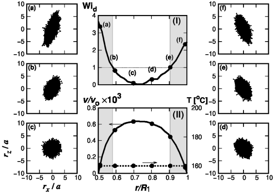
Figure 6: (I) Weissenberg number profile ${\sf Wi}_{\rm{d}}(r,T)$ defined by eq.(12) and (II) velocity and temperature profiles as functions of the radius at the steady state for (i) $T_{0}=160^{\circ}$C. The figures (a)-(f) are the superimposed images of polymer conformations in the fluid elements located at $\tilde{r}=$ (a) 0.52, (b) 0.60, (c) 0.71, (d) 0.81, (e) 0.92, and (f) 0.98, where the primitive paths are drawn by fixing the center of mass to the origin. The shaded regions in (I) and (II) represent the ones in which ${\sf Wi}_{\rm{d}}>1$.

Here, we focus on the relation between conformations of the polymer chains and the reptation-time-based Weissenberg number ${\sf Wi}_{\rm{d}}$, defined as

$${\sf Wi}_{\rm{d}}(r,T)=\tau_{\rm{d}}(T(r))\Bigr{|}{\partial v_{z}\over\partial r}\Bigr{|}.$$ (12)

${\sf Wi}_{\rm{d}}$ is expected to help guide us in considering how the extended polymer chain is oriented. If ${\sf Wi}_{\rm{d}}$ is larger than unity, the polymer chains are expected to be oriented along the flow direction. In Fig.6 and Fig.7, the Weissenberg number ${\sf Wi}_{\rm{d}}$ is plotted as a function of $r$ at steady-state flows for the two typical cases of (i) and (iii), respectively. Fig.6 and Fig.7 (a)-(f) also show conformations of the polymer chains expressed by primitive paths in fluid elements located at the six typical points in the tube for the cases of (i) and (iii) at the steady state. In addition, the velocity and temperature distribution are shown to visualize the relation between them and polymer conformations. The shaded regions in Fig.6 and Fig.7 (I) and (II) are the regions where ${\sf Wi}_{\rm{d}}>1$, in which chains are oriented along the $z$-direction by shear flows. The states of polymer chains at the six typical points are drawn in Fig.7(a)-(f) as in Fig.6. As shown in Fig.7 (I) and (II), because $\tau_{\rm{d}}$ becomes shorter as the temperature increases near the inner cylinder, the Weissenberg number becomes less than unity. Namely, in the high temperature region close to the inner cylinder, the relaxation rate of the chain orientation becomes faster than the shear rate in this region. Although the polymer chains in this region experience a high shear rate, the polymer chains are not oriented that much along the flow direction due to the Weissenberg number being less than unity in the above region. On the other hand, in the low temperature region close to the outer cylinder, the relaxation rate is relatively slow, and the Weissenberg number is larger than unity; therefore, the chains are oriented along the flow direction. From the results shown in Fig.6 and Fig.7, we can clearly see that the polymer chains are not necessarily oriented even at a high shear rate depending on the temperature condition. Namely, it can be said that the reptation-time-based Weissenberg number ${\sf Wi}_{\rm{d}}(r,T)$ is an effective measure for considering a local orientation of polymer chains, especially in the nonisothermal case.

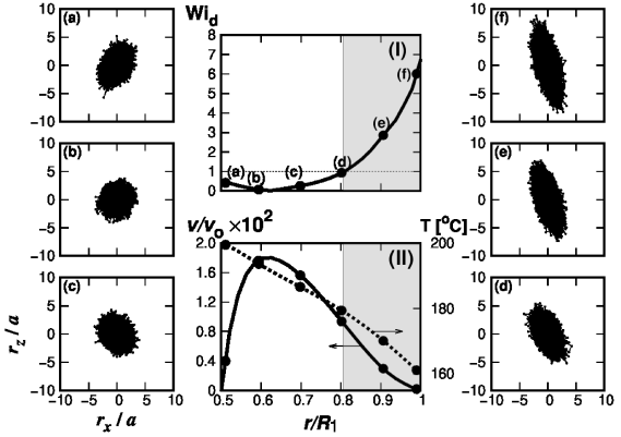
Figure 7: (I) Weissenberg number profile ${\sf Wi}_{\rm{d}}(r,T)$ defined by eq.(12) and (II) velocity and temperature profiles as functions of the radius at the steady state for (iii) $T_{0}=200^{\circ}$C. The figures (a)-(f) are the superimposed images of polymer conformations in the fluid elements located at $\tilde{r}=$ (a) 0.52, (b) 0.60, (c) 0.71, (d) 0.81, (e) 0.92, and (f) 0.98, where the primitive paths are drawn by fixing the center of mass to the origin. The shaded regions in (I) and (II) represent the ones in which ${\sf Wi}_{\rm{d}}>1$.

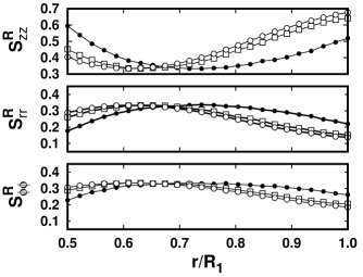
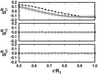
Figure 8: End-to-end tensor $S_{\alpha\beta}^{{\text{R}}}$ ($\alpha,\beta\in\{z,r,\phi\}$) as a function of $r/R_{1}$ for $T_{0}$ equal to (i) 160^∘C (filled circle), (ii) 180^∘C (open square), and (iii) 200^∘C (open circle).

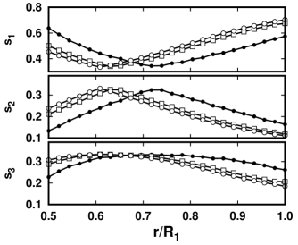
Figure 9: Eigenvalues of $\bm{S}^{{\text{R}}}$ for $T_{0}$ equal to (i) 160^∘C (filled circle), (ii) 180^∘C (open square), and (iii) 200^∘C (open circle). $s_{1}$, $s_{2}$ and $s_{3}$ are the eigenvalues whose eigenvectors are almost along the $z$-, $r$- and $\phi$-directions, respectively.

To quantitatively evaluate the microscopic states of polymer chains, we introduce the end-to-end tensor $\bm{S}^{{\text{R}}}$, defined as

$${\bm{S}}^{{\text{R}}}=\biggr{\langle}{1\over N_{\rm p}}\sum_{n=1}^{N_{\rm p}}{{\bm{R}}^{(n)}{\bm{R}}^{(n)}\over|{\bm{R}}^{(n)}|^{2}}\biggr{\rangle}$$ (13)

where ${\bm{R}}^{(n)}$ is the end-to-end vector of a polymer chain $n$ and $N_{\rm p}$ is the total number of polymer chains. $\langle(\cdots)\rangle$ denotes the ensemble average of $(\cdots)$, which is actually performed by taking a time average after the system reaches the steady state. Each component of the end-to-end tensor $\bm{S}^{{\text{R}}}$ in Fig.8 and eigenvalues of the tensor $\bm{S}^{{\text{R}}}$ in Fig.9 are plotted as functions of the radial position $r$ for the three cases (i)-(iii). Although $S_{zz}^{{\text{R}}}$, $S_{rr}^{{\text{R}}}$ or $S_{\phi\phi}^{{\text{R}}}$ can be described by the other two because of the relation $S_{zz}^{{\text{R}}}+S_{rr}^{{\text{R}}}+S_{\phi\phi}^{{\text{R}}}$ $=1$, all three are plotted for the purpose of comprehensibility. The tensor $\bm{S}^{{\text{R}}}$ is ${\bm{1}}/3$ in equilibrium, with $\bm{1}$ being the unit tensor. If $S_{\alpha\alpha}^{{\text{R}}}$ is larger than $1/3$, then the polymer chains are oriented along the $\alpha$-direction, but if it is less than $1/3$, then the chains are less-oriented along that direction. Because the eigenvectors to the eigenvalues $s_{1}$, $s_{2}$ and $s_{3}$ are almost along the $z$-, $r$- and $\phi$-directions, respectively, in similar way, $s_{\alpha}>1/3$ means that chains are oriented along the $\alpha$-direction. As seen from Fig.8 and Fig.9, $S_{zz}^{{\text{R}}}$ and $s_{1}$ are larger than 1/3, and therefore, the chains are highly oriented along the $z$-direction (flow direction), especially at places close to the walls. The tendency $s_{1}$ near a wall of the outer cylinder for the three cases can be understood by the velocity and its velocity gradient. At the region close to the wall of the inner cylinder, on the other hand, $s_{1}$ of case (i) is larger than those of the higher temperature cases (ii) and (iii), even though the velocity and velocity gradient of case (i) is significantly smaller than those of the other two cases (see Fig. 4(a)). The behaviors of $s_{2}$ for these three cases are opposite those of $s_{1}$. From the behavior of $s_{3}$, we can see that the chains are less-oriented along the $\phi$-direction and relatively gentle compared with those along the $r$-direction because the $\phi$-direction is the neutral direction. In addition, the correlations between the deformation along the $\phi$-direction and those along the other two directions, i.e., $S_{r\phi}^{{\text{R}}}$ and $S_{\phi z}^{{\text{R}}}$, are very small. We can see that the deformation correlation $S_{zr}^{{\text{R}}}$, on the other hand, is large. These results are in good agreement with the polymer conformation images shown in Fig. 6 and Fig. 7. It is clearly understood that the chain deformation at a position is determined not only by the local velocity gradient $\partial v_{z}/\partial r$ but also by the local-temperature-dependent relaxation time $\tau_{\rm d}(T(r))$, i.e., by the temperature dependent Weissenberg number ${\sf Wi}_{\rm{d}}(r,T)$ defined by eq.(12).

III.2 Dynamics after cessation of the external force density ($F_{\rm ext}=0$)

In the previous subsection, we investigated the steady state of the polymer melt flow between two coaxial cylinders under nonisothermal conditions. Here we focus on the dynamics of the polymer melt flow and its constituent polymer chains after cessation of the external force density. As the initial states for this investigation, we use the steady states (macroscopic flow and temperature distributions, and the microscopic state of the polymer chains in each fluid element) obtained for the three cases considered in the previous subsection, (i) $T_{0}=160^{\circ}$C, (ii) $T_{0}=180^{\circ}$C, and (iii) $T_{0}=200^{\circ}$C, with the time set to $\tilde{t}=0$ when the force density is ceased. The equations for the dynamics of the fluid velocity and temperature are also given by (5) and (6), respectively, but the apparent Reynolds number ${\sf Re}^{\rm(a)}$ and thermal Péclet number ${\sf Pe}^{\rm(a)}$ come into play in the dynamics, in addition to ${\sf Br}^{\rm(a)}$. As already mentioned, these three dimensionless parameters are evaluated to be ${\sf Re}^{\rm(a)}=1.1\times 10^{-2}$, ${\sf Pe}^{\rm(a)}=1.1\times 10^{5}$, and ${\sf Br}^{\rm(a)}=4.2\times 10^{4}$. The boundary conditions for the velocity and temperature are the same as those for the steady state, i.e., are also given by (3) and (4), respectively. The treatment of the microscopic dynamics of the polymer chains is the same as that described in Sec. II.2 and Appendix I.
Fig.10 shows the time evolution of the flow for the case (iii) $T_{0}=200^{\circ}$C after cessation of the external force density for two types of simulations: (A) the MSS for the polymer melt and (B) the simulation of a pure viscous fluid whose viscosity is given by eq.(10). Note that the velocity and temperature distributions at the steady state of (B) are the same as those of (A), as explained in Sec. III.1. Fig.11 shows the scaled volumetric flow rates $\tilde{q}$ as a function of time for all three cases (i)-(iii). This scaled volumetric flow rate $\tilde{q}=q/(v_{0}R_{1}^{2})$ is defined by the following equation as:

$$\tilde{q}=2\pi\int_{\tilde{R}_{0}}^{\tilde{R}_{1}}\tilde{v}_{z}(\tilde{r})\tilde{r}d\tilde{r}.$$ (14)

Figure 10: Time evolutions of the velocity after cessation of the external force, by setting $F_{\rm ext}=0$ in (A) the MSS system for case (iii) 200^∘C in Fig.4, and (B) the corresponding non-Newtonian fluid (Cross-WLF model) evaluated in Fig.4.

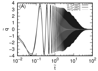
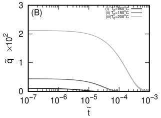
Figure 11: Scaled volumetric flow rates $\tilde{q}$ of (A) MSS and (B) the corresponding non-Newtonian fluid (Cross-WLF model) as a function of time for three different $T_{0}$ temperatures (i) $T_{0}=160^{\circ}$C, (ii) $T_{0}=180^{\circ}$C, and (iii) $T_{0}=200^{\circ}$C.

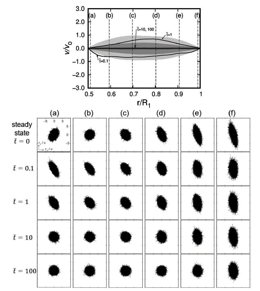
Figure 12: Velocity profiles for case (iii) at $\tilde{t}=0.1,1,10$, and $100$ in the top panel. The light, intermediate, and dark gray regions are drawn as the superposition of lines at $1<\tilde{t}\leq 2$, $2<\tilde{t}\leq 5$, and $5<\tilde{t}\leq 10$, respectively. In the bottom panel, local chain conformations at $\tilde{t}=0.1,1,10$, and $100$ in the fluid element located at the positions (a)-(f) in the top panel are shown.

We can see from Fig.10 and Fig.11 that the polymer melt systems (A) clearly exhibit an oscillatory flow behavior with a decaying amplitude, on the other hand, the pure viscous system (B) only shows a flow-decaying-behavior and reaches to a quiescent state in a short time. The flow behavior in (A) can be characterized by three quantities, the amplitude decay-time $\delta\tilde{t}_{\rm decay}^{\rm(viscoelastic)}$, the initial maximum amplitude $\cal A$, and the period of oscillation ${\cal T}_{\rm osc}$, whereas the flow behavior in (B) can be characterized solely by the decay-time $\delta\tilde{t}_{\rm decay}^{\rm(viscous)}$. From Fig.10(A) and Fig.11(A), we can see that the $\delta\tilde{t}_{\rm decay}^{\rm(viscoelastic)}$ for (i) $T_{0}=160^{\circ}$C, (ii) $T_{0}=180^{\circ}$C, and (iii) $T_{0}=200^{\circ}$C are approximately (i) 50, (ii) 20, and (iii) 5, respectively. From Fig.10(B) and Fig.11(B) we can see that $\delta\tilde{t}_{\rm decay}^{\rm(viscous)}\sim$ (i) $10^{-5}$, (ii) $10^{-4}$ and (iii) $10^{-3}$, and the decay-time becomes longer as $T_{0}$ increases, which is opposite to the $T_{0}$-dependence of the decay-time in (A). As explained in Appendix II, the short decay time in the pure viscous system (B) can be estimated by $\delta\tilde{t}_{\rm decay}^{\rm(viscous)}\sim{\sf Re}^{\rm(a)}/[(2\pi)^{2}\tilde{\eta}_{0}(\bar{T})]$, where $\bar{T}$ is an effective temperature. For example, if $\bar{T}$ is approximated to be the temperature of the inner wall, i.e., $\bar{T}\sim T_{0}$, the $\delta\tilde{t}_{\rm decay}^{\rm(viscous)}$ are roughly estimated as (i) $3.5\times 10^{-6}$, (ii) $0.97\times 10^{-4}$, and (iii) $1.0\times 10^{-3}$ by using $\tilde{\eta}_{0}(160^{\circ}$C$)\simeq 79$, $\tilde{\eta}_{0}(180^{\circ}$C$)\simeq 2.8$, $\tilde{\eta}_{0}(200^{\circ}$C$)\simeq 0.27$, and ${\sf Re}^{\rm(a)}\sim 1.1\times 10^{-2}$, and these estimated values are consistent with the results of the simulations mentioned above. Regarding the amplitude decay-time in the polymeric system, we can understand that the decay-time is approximately twice the polymer relaxation time, i.e., $2\tilde{\tau}_{\rm{d}}(T)\sim 2a_{T}\tilde{\tau}_{\rm{d}}(T_{\rm ref})$ as shown in Appendix II. So we can estimate $\delta\tilde{t}_{\rm decay}^{\rm(viscoelastic)}$ as (i) $2\tilde{\tau}_{\rm{d}}(160^{\circ}$C$)\simeq 732$, (ii) $2\tilde{\tau}_{\rm{d}}(180^{\circ}$C$)\simeq 25.6$ and (iii) $2\tilde{\tau}_{\rm{d}}(200^{\circ}$C$)\simeq 2.4$, which roughly grasps the tendency of the decay-times in (A). We can also understand the opposite tendency of the decay-time as a function of $T_{0}$ between (A) and (B) through the temperature dependence of $\eta_{0}(T)$ and $\tau_{\rm{d}}(T)$. It should be noted that the temperature distributions in both cases (A) and (B) show almost no change on the time scale of the flow decay ($\tilde{t}\lesssim\delta\tilde{t}_{\rm decay}^{\rm(viscoelastic)}$), with respect to the steady state temperature distribution shown in Fig.4(b), because of the very large thermal Péclet number ${\sf Pe}^{\rm(a)}$. The characteristic temperature relaxation time to the equilibrium distribution given in eq.(11) is estimated to be $\delta\tilde{t}_{\rm relax}^{(T)}\sim{\sf Pe}^{\rm(a)}\simeq 10^{5}$. The period of the oscillating flow $\tilde{\cal T}_{\rm osc}$ for case (iii) is evaluated visually to be $\tilde{\cal T}_{\rm osc}\simeq 0.2$ from Fig.10, and it can be found that those for the other two cases (i) and (ii) are almost the same, as seen from Fig.11(A). As given in Appendix II, the period is theoretically estimated to be $\tilde{\cal T}_{\rm osc}\simeq 2\pi/\tilde{\omega}_{1}$ where $\tilde{\omega}_{1}\equiv 2\pi[\tilde{\eta}_{0}(\bar{T})/{\sf Re}^{(\rm a)}\tilde{\tau}_{\rm{d}}(\bar{T})]^{1/2}$. By using this expression, the periods $\tilde{\cal T}_{\rm osc}$ for (i)-(iii) are evaluated to be (i) 0.23, (ii) 0.22, (iii) 0.21. Interestingly, the amplitude of the oscillating flow is approximately one hundred times larger than the magnitude of the flow at the steady-state. The large amplitude of the oscillation comes from the releasing of the stored elastic energy in the deformed polymer chains. The maximum amplitude ${\cal A}$ in the first oscillation after the cessation of $F_{\rm ext}$ is larger for smaller $T_{0}$, it can estimated theoretically as ${\cal A}\sim 4\tilde{F}_{\rm ext}/\left(\pi\tilde{\omega}_{1}(\bar{T}){\sf Re}^{(\rm a)}\right)$, and is evaluated to be (i) 2.71 (ii) 2.65 and (iii) 2.59, which is consistent with the results shown in Fig.10(A). This tendency can be attributed to the longer relaxation times for stretch and orientation of polymer chains at lower temperatures.
To understand the relation between the oscillatory flow and the chain deformation, the velocity profiles at $\tilde{t}=0.1$, $1$, $10$, and $100$ for case (iii) are plotted in the top panel of Fig.12. In addition, velocity profiles at $1<\tilde{t}\leq 2$, $2<\tilde{t}\leq 5$, and $5<\tilde{t}\leq 10$ are superimposed, which results in the light, intermediate and dark gray regions, respectively. In the bottom panes of Fig.12, local chain conformations at the positions corresponding to (a)-(f) in the top panel, and also in Fig.7, at $\tilde{t}=0,~{}~{}0.1,~{}~{}1,~{}10$, and $100$ are drawn by fixing the center of mass of each chain to the origin. At steady state ($\tilde{t}=0$), polymer chains close to the inner wall, (i.e.,(a)), are stretched along the flow direction and slightly tilted in the positive radial direction, located near the center region ((b) and (c)) are almost isotropic, and those close to the outer wall ((d), (e) and (f)) are highly stretched and tilted toward the inner side, because of the long relaxation time coming from the lower temperature of the outer wall. After the cessation of the external force, at first, elastic energy stored in the chains induces a backflow, as seen in Figs.10(A) and 11(A), with the chains oriented in the backflow direction at $\tilde{t}\lesssim 0.05$ (although we did not show the corresponding figures in Fig.12). At around $\tilde{t}\simeq 0.05$, the backflow starts decreasing and reverting to a flow in the positive direction. At $\tilde{t}=0.1$ it is still on its way back towards a positive flow, with the chains still oriented in the backflow direction, as can be seen in the second row of the chain conformation panels. At $\tilde{t}\simeq 0.16$, the velocity reaches a maximum positive flow. Then, the flow again exhibits a backflow and reaches the second largest backflow at $\tilde{t}=0.27$. After that, the oscillatory back- and forth- flow continue, with decreasing amplitude. Polymer chains located at almost all positions go back to the relaxed state at around a time between $\tilde{t}=1$ and $\tilde{t}=10$, except for the chains located close to the outer wall, because of the longer relaxation time ($\tilde{\tau}_{\rm{d}}(T_{1})\simeq 366$) at low temperatures ($T_{1}\simeq 160^{\circ}$C). Although the chain conformations close to the outer wall are still oriented, to a certain extent, the macroscopic flow has already decayed, as seen from Figs.10(A), 11(A) and 12 (top panel).

IV Conclusions

We investigated a well-entangled polymer melt flow under nonisothermal conditions by using a multiscale simulation method. Thus far, a multiscale simulation has been applied to isothermal flow problems; here, we extended the multiscale simulation method such that it is applicable to the nonisothermal flow problem. At the macroscopic level, the way to incorporate the effect of temperature into the macroscopic equations (momentum and energy balance equations) has already been well established, and the method can be directly applied to flow problems if the temperature-dependence of the density $\rho$, the specific heat capacity $C_{p}$, and the thermal conductivity $k$ and the stress tensor field $\bm{\sigma}$ are known, but at the microscopic level, the way to incorporate the effect into a coarse-grained microscopic model has not yet been clarified because the temperature dependence of the parameters used in this coarse-grained microscopic model is usually not known. It is well known that temperature effects can be incorporated into constitutive equations by scaling its parameters, based on the time-temperature superposition rule. Given this fact, we have used the same time-temperature superposition, in reverse, in order to extend the multiscale simulation method to nonisothermal flows. In this way, we are able to evaluate the temperature-dependent relaxation times and stresses needed for the slip-link simulations at the microscopic level.

To demonstrate the effectiveness of the method, we investigated macroscopic polymer melt flows and microscopic state polymer chains between two coaxial cylinders under nonisothermal conditions, in which we used a polymer melt composed of linear monodisperse polymer chains with $Z$-entanglement points ($Z=Z_{0}+1$, $Z_{0}$ is the number of strands, and $Z_{0}=10$) on a chain in equilibrium. The temperatures of the inner and the outer cylinders are respectively set to $T_{0}$ and $T_{1}$, and $T_{1}$ is always set to $T_{1}=160^{\circ}$C), while $T_{0}$ is set to (i) 160^∘C, (ii) 180^∘C, or (iii) 200^∘C. As a result, the extended method succeeds in simulating temperature-dependent flow behaviors and creating a relation between the macroscopic flow and temperature distribution in the tube and the microscopic states of the polymer chains along the radial direction. Although the polymer chains are stretched and oriented along the flow direction according the local shear rate, the degree of deformations of the polymer chains are determined not only by the local shear rate but also by the local temperature through the temperature-dependent relaxation times $\tau_{\rm{d}}$ and $\tau_{\text{R}}$.

At steady states under a constant external force, near the outer cylinder, the length of primitive path $L$ and the number of entanglements on a single chain $Z$ in the high-temperature cases (ii) and (iii) become longer and smaller than those in case (i), respectively. Near the inner cylinder, on the other hand, these quantities display opposite tendencies, although the magnitude of the shear rates in this region is larger than those in the region near the outer cylinder. These behaviors can be explained by considering the temperature-dependent reptation-time-based Weissenberg number ${\sf Wi}_{\rm{d}}(r,T)$, and therefore, the number is found to be a very effective parameter in understanding the microscopic state of polymer chains.

We also investigated the dynamics of the system after cessation of the external force, by using the steady state as an initial state. The flows of the polymeric system exhibit an oscillatory decaying flow, whereas the corresponding pure viscous system exhibits a simple decaying flow. We also demonstrated how the polymer conformations are related to the oscillatory decaying flow behavior.

In this paper, although we could not directly compare our numerical results with experimental ones, we are hoping to make intensive comparisons of the data obtained by the nonisothermal MSS and experimental data in the future, not only from the viewpoint of the macroscopic properties, such as the flow and temperature distributions, but also from the microscopic state of the polymer chains. We will continue to apply the present method to more industrially oriented problems to predict the temperature-dependent flow behavior and microscopic state of a polymer chain. Finally, we believe that the present method offers us a new idea and/or novel knowledge not only on macroscopic flow but also a microscopic state of polymer chains under nonisothermal conditions.

References

- (1) Masubuchi Y, (2014) Simulating the Flow of Entangled Polymers. Annu Rev Chem Biomol Eng 5: 11—-33.
- (2) Sato T, (2020) A Review on Transport Phenomena of Polymeric Liquids. J Soc Rheol Jpn 48: 1—-14.
- (3) Bird R B, Armstrong R C, Hassager O, (1987), Dynamics of Polymeric Liquids Volume 1 Fluid Mechanics, 3 Eds., John Wiley & Sons, Inc.
- (4) Cross M M, (1965), Rheology of non-Newtonian fluids: A new flow equation for pseudoplastic systems. J Colloid Sci, 20: 417—-437.
- (5) Ferry J D, (1980), Viscoelastic Properties of Polymers, 3 Eds., John Wiley & Sons, Inc.
- (6) Chiang H H, Hieber C A, Wang K K, (1991) A Unified Simulation of the Filling and Postfilling Stages in Injection Molding. Part I: Formulation. Polym Eng Sci 31: 116—-124.
- (7) Otmani R E, Zinet M, Boutaous M, Benhadid H, (2011) Numerical Simulation and Thermal Analysis of the Filling Stage in the Injection Molding Process: Role of the Mold-Polymer Interface. J Appl Polym Sci 121: 1579—-1592.
- (8) Khalifeh A, Clermont J-R, (2005) Numerical simulations of non-isothermal three-dimensional flows in an extruder by a finite-volume method. J Non-Newton Fluid Mech 126: 7—-22.
- (9) Zdanski P S B, Vaz Jr M, (2009) Three-dimensional polymer melt flow in sudden expansions: Non-isothermal flow topology. Int J Heat Mass Transf 52: 3585—-3594.
- (10) Doufas A K, McHugh A J, Miller C, (2000) Simulation of melt spinning including flow-induced crystallization Part I. Model development and predictions. J Non-Newton Fluid Mech 92: 27—-66.
- (11) Peters G W M, Baaijens F P T, (1997) Modeling of non-isothermal viscoelastic flows. J Non-Newton Fluid Mech 68: 205—-224.
- (12) Kunisch K, Marduel X, (2000) Optimal control of non-isothermal viscoelastic fluid flow. J Non-Newton Fluid Mech 88: 261—-301.
- (13) Wachs A, Clermont J-R, (2000) Non-isothermal viscoelastic flow computations in an axisymmetric contraction at high Weissenberg numbers by a finite volume method. J Non-Newton Fluid Mech 95: 147—-184.
- (14) Laso, M, Öttinger H C, (1993) Calculation of viscoelastic flow using molecular models: the CONNFFESSIT approach. J Non-Newton Fluid Mech 47: 1—-20.
- (15) Keunings R, (2004) Micro-macro methods for the multiscale simulation of viscoelastic flow using molecular models of kinetic theory. Rheology Reviews 2004, Binding D M and Walters K (Eds.), The British Society of Rheology, 67—-98.
- (16) Hulsen M A, van Heel A P G, van den Brule B H A A, (1997) Simulation of viscoelastic flows using Brownian configuration fields. J Non-Newton Fluid Mech 70: 79—-101.
- (17) Halin P, Lielens G, Keunings R, Legat V, (1998) The Lagrangian particle method for macroscopic and micro-macro viscoelastic flow computations. J Non-Newton Fluid Mech 79: 387—-403.
- (18) E W, Engquist B, (2003) The Heterogeneous Multiscale Methods. Commun Math Sci 1: 87—-132.
- (19) Yasuda S, Yamamoto R, (2008) A model for hybrid simulations of molecular dynamics and computational fluid dynamics. Phys Fluids 20: 113101.
- (20) Murashima T, Taniguchi T, (2010) Multiscale Lagrangian Fluid Dynamics Simulation for Polymeric Fluid. J Polym Sci B Polym Phys 48: 886—-893.
- (21) Murashima T, Taniguchi T, (2011) Multiscale simulation of history-dependent flow in entangled polymer melts. Europhys Lett 96: 18002.
- (22) Murashima T, Taniguchi T, (2012) Flow-History-Dependent Behavior of Entangled Polymer Melt Flow Analyzed by Multiscale Simulation. Journal of the Physical Society of Japan 81 SA013,
- (23) Sato T, Harada K, Taniguchi T, (2019) Multiscale Simulations of Flows of a Well-Entangled Polymer Melt in a Contraction-Expansion Channel. Macromolecules 52: 547—-564.
- (24) Sato T, Taniguchi T, (2017) Multiscale simulations for entangled polymer melt spinning process. J Non-Newton Fluid Mech 241: 34—-42.
- (25) Doi M, Takimoto J, (2003) Molecular modeling of entanglement. Phil Trans R Soc Lond A 361: 641—-652.
- (26) Kremer K, Grest G S, (1990) Dynamics of entangled linear polymer melts: A molecular-dynamics simulation. J Chem Phys 92: 5057—-5086.
- (27) Yasuda S, Yamamoto R, (2014) Synchronized Molecular-Dynamics Simulation via Macroscopic Heat and Momentum Transfer: An Application to Polymer Lubrication. Phys Rev X 4: 041011.
- (28) Yasuda S, Yamamoto R, (2016) Synchronized molecular-dynamics simulation for the thermal lubrication of a polymeric liquid between parallel plates. Comput Fluids 124: 185—-189.
- (29) Yasuda S, (2019) Synchronized Molecular-Dynamics Simulation of the Thermal Lubrication of an Entangled Polymeric Liquid. Polymers 11: 131.
- (30) Sato T, Taniguchi T, (2019) Rheology and Entanglement Structure of Well-Entangled Polymer Melts: A Slip-Link Simulation Study. Macromolecules 52: 3951—-3964.
- (31) Habla F, Woitalka A, Neuner S, Hinrichsen O, (2012) Development of a methodology for numerical simulation of non-isothermal viscoelastic fluid flows with application to axisymmetric 4:1 contraction flows. Chem Eng J 207-208: 772—-784.
- (32) Pol H, Banik S, Azad B L, Thete S, Doshi P, Lele A, (2014) Nonisothermal analysis of extrusion film casting process using molecular constitutive equations. Rheol Acta 53: 85—-101.
- (33) Zatloukal M (2016) Measurements and modeling of temperature-strain rate dependent uniaxial and planar extensional viscosities for branched LDPE polymer melt. Polymer 104: 258—-267.
- (34) Zhuang X, Ouyang J, Li W, Li Y, (2017) Three-dimensional simulations of non-isothermal transient flow and flow-induced stresses during the viscoelastic fluid filling process. Int J Heat Mass Transfer 104: 374—-391.
- (35) Gao P, Wang X, Ouyang J, (2019) Numerical investigation of non-isothermal viscoelastic filling process by a coupled finite element and discontinuous Galerkin method. Int J Heat Mass Transfer 140: 227—-242.
- (36) Doi M, Edwards S F, (1986), The Theory of Polymer Dynamics, Oxford University Press.
- (37) Marrucci G, (1996) Dynamics of entanglements: A nonlinear model consistent with the Cox-Merz rule. J Non-Newton Fluid Mech 62: 279—-289.