Einstein@Home Discovery of the Gamma-ray Millisecond Pulsar PSR J2039$-$5617 Confirms Its Predicted Redback Nature

Abstract

The Fermi Large Area Telescope gamma-ray source 3FGL J2039.6$-$5618 contains a periodic optical and X-ray source that was predicted to be a “redback” millisecond pulsar (MSP) binary system. However, the conclusive identification required the detection of pulsations from the putative MSP. To better constrain the orbital parameters for a directed search for gamma-ray pulsations, we obtained new optical light curves in 2017 and 2018, which revealed long-term variability from the companion star. The resulting orbital parameter constraints were used to perform a targeted gamma-ray pulsation search using the Einstein@Home distributed volunteer computing system. This search discovered pulsations with a period of $2.65$ ms, confirming the source as a binary MSP now known as PSR J2039$-$5617. Optical light curve modelling is complicated, and likely biased, by asymmetric heating on the companion star and long-term variability, but we find an inclination $i\gtrsim$ 60 $\degr$, for a low pulsar mass between $1.1\,M_{\odot}<M_{\rm psr}<$ 1.6 $M_{\odot}$, and a companion mass of $0.15$–$0.22\,M_{\odot}$, confirming the redback classification. Timing the gamma-ray pulsations also revealed significant variability in the orbital period, which we find to be consistent with quadrupole moment variations in the companion star, suggestive of convective activity. We also find that the pulsed flux is modulated at the orbital period, potentially due to inverse Compton scattering between high-energy leptons in the pulsar wind and the companion star’s optical photon field.

1 Introduction

Millisecond pulsars (MSPs) are old neutron stars that have been spun-up to millisecond rotation periods by the accretion of matter from an orbiting companion star (Alpar et al., 1982). The most compelling evidence for this “recycling” scenario comes from the discovery of three transitional MSPs, which have been seen to switch between rotationally powered MSP and accretion-powered low-mass X-ray binary (LMXB) states (Archibald et al., 2009; Papitto et al., 2013; Bassa et al., 2014; Stappers et al., 2014). In their rotationally powered states, these transitional systems all belong to a class of interacting binary MSPs known as “redbacks”, which are systems containing an MSP in orbit with a low-mass ($0.1\,M_{\odot}\lesssim M\lesssim 0.4\,M_{\odot}$) non-degenerate companion star (Roberts, 2013). Redbacks, and the closely related “black widows” (which have partially degenerate companions with $M\lesssim 0.05\,M_{\odot}$), are named after species of spiders in which the heavy females have been observed to consume the smaller males after mating, reflecting the fact that the lighter companion stars are being destroyed by the pulsar’s particle wind and/or intense high-energy radiation.

Until recently, only a handful of these “spider” systems had been found in radio pulsar surveys of the Galactic field. This is most likely due to the ablation phenomenon which gives redbacks and black widows their nicknames: plasma from the companion can eclipse, scatter and disperse the MSP’s radio pulsations for large fractions of an orbit (e.g., Ray et al., 2013; Deneva et al., 2016), causing these pulsars to be easily missed in radio pulsar surveys. In addition, traditional “acceleration” search methods for binary pulsars (Ransom et al., 2002) are only optimal when the integration time is $\lesssim 10\%$ of the orbital period, leading to an additional sensitivity loss to spiders, which often have orbital periods of just a few hours.

Fortunately, gamma-ray emission from an MSP does not suffer from strong propagation effects from intrabinary plasma structures. A new route for binary MSP discoveries therefore appeared with the launch of the Fermi Gamma-ray Space Telescope in 2008. The on-board Large Area Telescope (LAT) discovered gamma-ray pulsations from a number of known MSPs shortly after launch (Abdo et al., 2009). Targeted radio observations of unidentified, but pulsar-like Fermi-LAT sources have since discovered more than 90 new MSPs, more than a quarter of all known MSPs in the Galactic field. A disproportionately large fraction of these are spiders that had been missed by previous radio surveys (Ray et al., 2012).

In addition to the large number of radio-detected spiders found in Fermi-LAT sources, a growing number of candidate spiders have been discovered through searches for optical and X-ray counterparts to gamma-ray sources (e.g., Romani et al., 2014; Strader et al., 2014; Halpern et al., 2017; Salvetti et al., 2017; Li et al., 2018). In a few cases, the MSP nature of these sources was confirmed by the detection of radio or gamma-ray pulsations (Pletsch et al., 2012; Ray et al., 2020), however most of these candidates remain unconfirmed.

To overcome the difficulties in detecting spider MSPs in radio pulsation searches, it is possible to directly search for gamma-ray pulsations in the LAT data. In contrast to searches for isolated MSPs, which can be detected in gamma-ray pulsation searches without any prior knowledge of the parameters (Clark et al., 2018), gamma-ray pulsation searches for binary MSPs require tight constraints on the orbital parameters of the candidate binary system to account for the orbital Doppler shift (Pletsch et al., 2012), which would smear out the pulsed signal if not corrected for. This in turn requires long-term monitoring of the companion star’s optical light curve to measure the orbital period with sufficient precision, and spectroscopic radial velocity measurements and/or light curve modelling to tie the photometric light curve to the pulsar’s kinematic orbital phase. Prior to this work, such searches have been successful only twice (Pletsch et al., 2012; Nieder et al., 2020b), with both MSPs being extremely compact black widow systems with small orbital Doppler modulations.

Salvetti et al. (2015) and Romani (2015) discovered a high-confidence candidate redback system in the bright, pulsar-like gamma-ray source 3FGL J2039.6$-$5618 (Acero et al., 2015). This source is now known as 4FGL J2039.5$-$5617 in the latest Fermi-LAT Fourth Source Catalog (hereafter 4FGL, Abdollahi et al., 2020). This system (which we refer to hereafter as J2039) contains a periodic X-ray and optical source with orbital period $P_{\rm orb}\approx 5.5$ hr. The optical light curve exhibits two “ellipsoidal” peaks, interpreted as a tidally distorted companion star in an intense gravitational field being viewed from the side, where its projected surface area is highest. These peaks have unequal amplitudes, indicating a temperature difference between the leading and trailing sides of the star. Despite the high likelihood of this source being a redback system, the pulsar remained undetected in repeated observations attempting to detect its radio pulsations by Camilo et al. (2015).

On 2017 June 18, we took new observations of J2039 with the ULTRACAM (Dhillon et al., 2007) high-speed multi-band imager on the 3.5m New Technology Telescope (NTT) at ESO La Silla. The goal of these observations was to refine the orbital period uncertainty by phase-aligning a new orbital light curve with the 2014 GROND observations from Salvetti et al. (2015). However, we found that the optical light curve had changed significantly. Further observations obtained on 2018 June 02 also found a light curve that differed from the first two. This variability, similar to that discovered recently in other redback pulsars (van Staden & Antoniadis, 2016; Cho et al., 2018), poses challenges for obtaining reliable estimates of the physical properties such as the binary inclination angle and pulsar mass via optical light curve modelling (e.g., Breton et al., 2012; Draghis et al., 2019).

Using constraints on the pulsar’s orbital period and epoch of ascending node from preliminary models fit to the optical data, we performed a gamma-ray pulsation search using the Einstein@Home distributed volunteer computing system (Knispel et al., 2010; Allen et al., 2013), which finally identified the millisecond pulsar, now named PSR J2039$-$5617, at the heart of the system.

In this paper, we present the detection and timing of gamma-ray pulsations from PSR J2039$-$5617, and our new optical observations of the system. The paper is organised as follows: in Section 2 we review the literature on recent observations of the system to update our knowledge of its properties; Section 3 presents updated analysis of Fermi-LAT gamma-ray observations of 4FGL J2039.5$-$5617, and describes the gamma-ray pulsation search, discovery and timing of PSR J2039$-$5617; in Section 4 we describe the newly obtained optical data, and model the optical light curves to estimate physical properties of the system and investigate the observed variability; in Section 5 we discuss the newly clarified picture of PSR J2039$-$5617 in the context of recent observations of redback systems; and finally a brief summary of our results is given in Section 6.

Shortly after the discovery of gamma-ray pulsations reported in this paper, the initial timing ephemeris was used to fold existing radio observations taken by the CSIRO Parkes radio telescope. The resulting detections of radio pulsations and orbital eclipses are presented in a companion paper (Corongiu, A. et al. 2020, MNRAS, accepted.), hereafter Paper II.

2 Summary of previous literature

The periodic optical counterpart to 4FGL J2039.5$-$5617 was discovered by Salvetti et al. (2015) and Romani (2015) in photometric observations of the gamma-ray source region taken over three nights on 2014 June 16–18 with GROND (Greiner et al., 2008) on the ESO/MPG 2.2m telescope on La Silla. These observations covered SDSS $g^{\prime},r^{\prime},i^{\prime}$, and $z^{\prime}$ optical filters in simultaneous $115$ s exposures, and $H$, $J$, and $K$ near infrared filters in simultaneous $10$ s exposures. For consistency with the new optical light curves presented in this paper, we re-reduced the optical observations but chose not to include the infrared observations, which were not compatible with our reduction pipeline. These observations revealed a double-peaked light curve typical of redback systems, but with the peak corresponding to the companion’s ascending node brighter and bluer than that of the descending node. This requires the trailing side of the star to be hotter than the leading side, perhaps due to heating flux being redirected by an asymmetric intra-binary shock (e.g., Romani & Sanchez, 2016), or due to the presence of cold spots on the leading edge (e.g., van Staden & Antoniadis, 2016).

Salvetti et al. (2015) and Romani (2015) also analyzed X-ray observations of J2039 taken by XMM-Newton. These data had insufficient time resolution to test for millisecond X-ray pulsations, but did reveal a periodic ($\sim 5.5$ hr) modulation in the X-ray flux, which the authors identified as likely being due to synchrotron emission from particles accelerated along an intra-binary shock, commonly seen in black widow and redback systems. However, without long-term timing to precisely measure the orbital period the authors were unable to unambiguously phase-align the optical and X-ray light curves. The Catalina Surveys Southern Periodic Variable Star Catalogue (Drake et al., 2017) includes 223 photometric observations of J2039 between 2005 and 2010. While the uncertainties on these unfiltered data are too large for a detailed study of the light curve over these 5 years, the underlying periodicity is clearly recovered by a 2-harmonic Lomb Scargle periodogram, which reveals a significant signal with an orbital period of $P_{\rm orb}=0.227980(1)$ d with no significant aliases. Folding at this period shows that the X-ray modulation peaks at the putative pulsar’s inferior conjunction, indicating that the shock wraps around the pulsar. This scenario requires the companion’s outflowing wind to overpower the pulsar wind (see e.g. Romani & Sanchez, 2016; Wadiasingh et al., 2017).

Using 9.5 yr of Fermi-LAT data, Ng et al. (2018) discovered that the gamma-ray emission from J2039 contains a component below $3$ GeV that is modulated at the orbital period, peaking around the companion star’s inferior conjunction, i.e. half an orbit out of phase with the X-ray modulation. This phase offset rules out synchrotron emission from particles accelerated along the shock front as an origin for the gamma-ray flux, as such a component would occur at the same orbital phase as the X-ray modulation. Instead, Ng et al. (2018) propose that this component is produced by inverse Compton scattering between the pulsar’s high-energy particle wind and the companion star’s optical photon flux. Such a component would be strongest if our line of sight to the pulsar passes close to the limb of the companion star, suggesting an intermediate inclination angle $i\sim 80\degr$.

Strader et al. (2019) obtained spectroscopic observations with the Goodman Spectrograph (Clemens et al., 2004) on the SOAR telescope. The spectra suggest a mid-G-type companion star, with temperature $T\approx 5500$ K and variations of up to $\pm 200$ K across the orbit attributed to heating from the pulsar. The spectroscopy also revealed a single-line radial velocity curve whose semi-amplitude of $K_{\rm c}=324\pm 5$ km s^-1 implies an unseen primary with a minimum mass $M>0.8M_{\odot}$. Strader et al. (2019) modelled the GROND light curve, incorporating two large cold spots on the outer face of the companion star to account for the light curve asymmetry, and found an inclination angle $i\sim 55\degree$, from which they deduce a heavy neutron star primary with $M\gtrsim 1.8M_{\odot}$.

The optical counterpart is also covered in the Second Gaia Data Release (DR2, Gaia Collaboration et al., 2016, 2018). Using Equation (2) of Jordi et al. (2010), the Gaia DR2 colour $G_{\rm BP}-G_{\rm RP}=1.02$ implies an effective temperature of $T_{\rm eff}=5423\pm 249$ K, consistent with the spectroscopic temperature measured by Strader et al. (2019). The Gaia DR2 also provides a marginal parallax detection ($\varpi=0.40\pm 0.23$ mas) for a minimum ($95\%$ confidence) distance of $d>1.2$ kpc, and a total proper motion of $\mu=15.51\pm 0.26$  mas yr^-1, corresponding to a distance-dependent transverse velocity of $v(d)\approx 75\,(d/1\,\textrm{kpc})$ km s^-1. The systemic velocity (the radial velocity of the binary centre of mass) measured from optical spectroscopy by Strader et al. (2019) is just $6\pm 3\,$km s^-1 indicating that the 3D velocity vector is almost entirely transverse.

3 Gamma-ray Observations

To update the gamma-ray analysis of J2039 from previous works (Salvetti et al., 2015; Ng et al., 2018), we selected SOURCE-class gamma-ray photons detected by the Fermi LAT between 2008 August 04 and 2019 September 12. Photons were included from within a $15\degree$ region of interest (RoI) around J2039, with energies greater than $100\,$MeV, and with a maximum zenith angle of $90\degree$, according to the “Pass 8” P8R3_SOURCE_V2 (Atwood et al., 2012; Bruel et al., 2018) instrument response functions (IRFs) .

We first investigated the gamma-ray spectral properties of 4FGL J2039.5$-$5617. We used the 4FGL catalogue as an initial model for the RoI, and used the gll_iem_v07.fits and iso_P8R3_SOURCE_V2_v1.txt models to describe the Galactic and isotropic diffuse emission, respectively. We replaced 4FGL J2039.5$-$5617 in the RoI model with a point source at the Gaia DR2 position of the optical source. To model the source spectrum, we used a subexponentially-cutoff power-law spectrum typical for gamma-ray pulsars (4FGL),

$$\frac{dN}{dE}=K\left(\frac{E}{E_{0}}\right)^{-\Gamma}\exp\,\left(-a\left(\frac{E}{1\,{\rm MeV}}\right)^{b}\right)\,,$$ (1)

where the parameters $E_{0}=1$ GeV (“pivot energy”) and $b=2/3$ (exponential index) were fixed at their 4FGL values, while the parameters $K$ (normalisation), $\Gamma$ (low-energy spectral index) and $a$ (exponential factor) were free to vary during fitting. We performed a binned likelihood analysis using fermipy (Wood et al., 2017) version 0.18.0, with $0.05\degree\times 0.05\degree$ bins and 10 logarithmic energy bins per decade. For this analysis we utilised the “PSF” event types and corresponding IRFs, which partition the LAT data into quartiles based on the quality of the reconstructed photon arrival directions. All 4FGL sources within $25\degree$ of the optical counterpart position were included in the model. Using the “optimize” function of fermipy, the parameters of all sources in the region were updated from their 4FGL values one at a time to find a good starting point. We then performed a full fit for the region surrounding J2039. The spectral parameters of all sources within $10\degree$ were free to vary in the fitting, as were the normalisations of the diffuse models and the spectral index of the Galactic diffuse model.

The gamma-ray source at the location of the optical counterpart is detected with test statistic $\textrm{TS}=2167$ (the TS is defined as twice the increase in log-likelihood when the source is added to the model). The spectrum has a photon power-law index of $\Gamma=1.4\pm 0.1$ and an exponential factor of $a=(7\pm 1)\times 10^{-3}$. The total energy flux above $100$ MeV is $G_{\gamma}=(1.46\pm 0.06)\times 10^{-11}$ erg cm^-2 s^-1. At an assumed distance of $1.7$ kpc (from our optical light-curve modelling in Section 4.2), this gives a gamma-ray luminosity of $L_{\gamma}=(5.0\pm 0.6)\times 10^{33}$ erg s^-1, assuming isotropic emission.

In gamma-ray pulsation analyses, photon weights are used to weight the contribution of each photon to a pulsation detection statistic to increase its sensitivity, and avoid the need for hard cuts on photon energy and incidence angle (Kerr, 2011). A weight $w_{j}$ represents the probability that the $j$-th photon was emitted by a target source, as opposed to by a fore/background source, based on the reconstructed photon energy and arrival direction, and a model for gamma-ray sources within the RoI. We computed these weights for photons whose arrival directions were within $5\degr$ of J2039 using gtsrcprob, again making use of the PSF event types. Within this region, there were $181,813$ photons in total, with $\sum_{j}w_{j}=3850$ “effective” photons. To speed up our timing analyses (Section 3.2) we additionally removed photons with $w<0.1$, leaving $6571$ photons which account for $93$% of the expected pulsation signal-to-noise ratio (which is proportional to $\sum_{j}w_{j}^{2}$, Clark et al., 2017).

The data set described above was used for the timing (Section 3.2) and orbital modulation analyses (Section 3.3) presented in this paper. For the pulsation search described in Section 3.1, we used an earlier data set which only covered data up to 2019 January 10 and used spectral parameters from a preliminary version of the 4FGL catalogue when computing photon weights.

3.1 Gamma-ray Pulsation Search

Using the hierarchical search methods described by Pletsch & Clark (2014), extended to provide sensitivity to binary pulsars by Nieder et al. (2020a), we performed a search for gamma-ray pulsations in the weighted Fermi-LAT photon arrival times.

For this, it was necessary to search for an unknown spin frequency $\nu$, spin-down rate $\dot{\nu}$, as well as the orbital period $P_{\rm orb}$, pulsar’s time of ascending node $T_{\rm asc}$, and pulsar’s projected semi-major axis $x=A_{\rm psr}\sin i$, where $A_{\rm psr}$ is the (non-projected) semi-major axis, and $i$ is the binary inclination angle. We did not search a range of sky positions as we used the precise Gaia position of the optical counterpart.

This 5-dimensional parameter volume is extremely large, and requires large computing resources and efficient algorithms to cover. To meet the large computational cost of the searches, we utilised the distributed volunteer computing system, Einstein@Home (Knispel et al., 2010; Allen et al., 2013). Under this system, the parameter space is split into millions of smaller chunks which can be searched by a typical personal computer within a few hours. These “work units” are computed while volunteer’s computers are otherwise idle. We also ported our Einstein@Home search code from CPUs to GPUs, which has previously been done for radio pulsar searches (Allen et al., 2013). The approximately 10,000 GPUs active on Einstein@Home increase the computing speed by an order of magnitude.

Despite this large computational resource, major efficiency gains and compromises are required to ensure that the computational effort of the search remains feasible. Key to improved efficiency is ensuring that the parameter space is covered by a grid of search locations that is as sparse as possible, yet sufficiently covers the volume to avoid missing signals. The required density is described by a distance metric – a function relating parameter space offsets to a corresponding expected loss in signal strength. This metric is described by Nieder et al. (2020a).

In the binary pulsar search, the spin parameters are searched in the same way as they are in isolated pulsar searches (see, e.g., Clark et al., 2017). $\nu$ is searched via Fast Fourier Transforms (FFTs). The relevant range in $\dot{\nu}$ is covered by a frequency-independent lattice.

The computational effort to search the orbital parameters depends linearly on the number of grid points. Searching the orbital parameters in a uniformly-spaced grid would be inefficient because the required metric spacing depends strongly on $\nu$ and $x$, i.e. at higher values for $\nu$ and $x$ the grid needs to be denser (Nieder et al., 2020a). To deal with the $\nu$-dependency, we break down the search into discrete $8$ Hz bands which are searched separately, and in each band the grid over the orbital parameters is designed to be dense enough for the maximum frequency in the band.

The orbital grid would be optimal if it has the lowest number of grid points such that each point in the parameter space is “covered”. A location in the parameter space is covered if the distance to the closest grid point is less than a chosen maximum. In inhomogeneous parameter spaces, the optimal grid is unknown. However, the required number of grid points $N_{\rm opt}$ for such a grid can be estimated using the distance metric under the assumption that locally the parameter space is sufficiently flat.

To search the inhomogeneous ($x$-dependent) orbital-parameter space efficiently, optimised grids are used (Fehrmann & Pletsch, 2014). These are built from stochastic grids, which are grids where grid points are placed stochastically while no two grid points are allowed to be closer than a minimum distance (Harry et al., 2009). We create a stochastic grid with $N_{\rm opt}$ grid points and optimise it by nudging the position of each grid point one by one towards “uncovered space” using a neighbouring cell algorithm (Fehrmann & Pletsch, 2014). After a few nudging iterations over all grid points the covering is typically sufficient for the search.

Using preliminary results from our optical modelling (see Section 4.2), obtained prior to the publication by Strader et al. (2019) of spectroscopic radial velocities which better constrain $T_{\rm asc}$, we constrained our orbital search space to $P_{\rm orb}=0.2279799(3)\,$d and $T_{\rm asc}=\textrm{MJD}~{}56884.9678(8)$. The range of expected $x$ values was not well constrained by this model, and as the computing cost increases with $x^{3}$ we chose to initially search up to $x=0.5$ lt-s, with the intention of searching to higher values should the search be unsuccessful.

The search revealed a signal with $\nu\approx 377$ Hz that was highly significant in both the initial semi-coherent and fully coherent follow-up search stages. The signal had $x\approx 0.47$ lt-s, which along with the companion’s radial velocity measurements by Strader et al. (2019) gives a mass ratio of $q=M_{\rm psr}/M_{\rm c}=K_{\rm c}P_{\rm orb}/2\pi x\approx 7.2$, and a minimum companion mass of $M_{\rm c}>0.15\,M_{\odot}$ assuming $i=90\degr$. These features conclusively confirm that the source is indeed a redback millisecond pulsar system, which can now be named PSR J2039$-$5617.

3.2 Gamma-ray Timing

Following the discovery of gamma-ray pulsations, we used the Fermi-LAT data set to obtain a rotational ephemeris spanning 11 years. To do so, we followed the principles described by Kerr et al. (2015), in which a template pulse profile $F(\phi)$ is produced, and the parameters $\boldsymbol{\lambda}$ of a phase model $\phi(t\,|\,\boldsymbol{\lambda})$, are fit to maximise the Poisson log-likelihood of the unbinned photon phases. Assuming that the weights derived in Section 3 represent the probability that each photon was emitted by the pulsar, then the contribution to the pulsation log-likelihood from the $j$-th photon, with weight $w_{j}$, is a mixture model between a constant (i.e. uniform in phase) background rate and the template pulse profile, with mixture weights of $1-w_{j}$ and $w_{j}$ respectively. Hence, the overall log-likelihood is

$$\log L(\boldsymbol{\lambda}\,|\,t_{j},w_{j},F)=\sum_{j=1}^{N}\log\left[w_{j}F\left(\phi\left(t_{j}\,|\,\boldsymbol{\lambda}\right)\right)+(1-w_{j})\right]$$ (2)

where $t_{j}$ denotes the measured arrival time of the $j$-th detected gamma-ray photon.

Folding the LAT data with the initial discovery ephemeris showed that the signal was not phase-connected over the entire data span, with the pulse profile drifting in and out of focus, indicative of a varying orbital period. Such effects are common among redback pulsars, and are attributed to variations in the quadrupole moment of the companion star coupling with the orbital angular momentum (e.g., Arzoumanian et al., 1994; Lazaridis et al., 2011; Pletsch & Clark, 2015). These effects significantly complicate efforts to time redbacks over more than a few months (e.g., Deneva et al., 2016).

In previous works, these effects have been accounted for by adding a Taylor series expansion of the orbital frequency perturbations to the constant-period orbital phase model, where the derivatives of the orbital angular frequency become additional parameters in the timing model. However, this parameterisation has a number of drawbacks. Large correlations between the orbital frequency derivatives greatly increase the time required for a Markov Chain Monte Carlo (MCMC) sampling procedure, which suffers from inefficient sampling and exploration during the “burn-in” phase for highly correlated parameter spaces. The Taylor series model also has poor predictive power as the orbital phase model “blows up” when extrapolating beyond the fit interval, making it difficult to extend an existing timing solution to incorporate new data. An astrophysical interpretation of the resulting timing solution is also not straightforward, as the measured orbital frequency derivatives depend on one’s choice of reference epoch ($T_{\rm asc}$), and are not representative of long-term trends in $P_{\rm orb}$ due to e.g. mass loss from the system.

These problems are very similar to those encountered when timing young pulsars with strong “timing noise”: unpredictable variations in the spin frequency over time. To address these issues, modern timing analyses treat timing noise as a stationary noise process, i.e. a random process with a constant correlation function, on top of the long-term spin-down due to the pulsar’s braking (Coles et al., 2011).

Kerr et al. (2015) used this method to time gamma-ray pulsars using Fermi-LAT data. To do this, a template pulse profile is constructed and cross correlated with the photon phases within weeks- or months-long segments to obtain a discrete pulse phase measurement, or “time-of-arrival” (TOA), for each segment, and the stochastic noise process is fit to these phase measurements. Timing parameters can then be fit analytically to minimise the chi-square log-likelihood of the covariance-transformed TOA residuals including a Bayesian penalty factor for the required timing noise process. However, this procedure has the drawback that for faint pulsars the segment length required to obtain a significant TOA measurement can become very long, and phase variations due to timing noise within each segment can no longer be neglected. Of course, the timing noise within a segment cannot be accounted for without a description of the noise process, which in turn cannot be obtained without the TOAs, creating a circular problem.

While this circular problem can be partially overcome by fitting iteratively, we have developed a new method to fit the noise process using every individual photon, rather than obtaining and fitting discrete TOAs. To obtain this best-fitting function and its uncertainty, we apply the sparse online Gaussian process (SOGP) procedure developed by Csató & Opper (2002). For purely Gaussian likelihoods, the Gaussian process framework would allow an exact posterior distribution for the noise process to be computed analytically (Rasmussen & Williams, 2005). In our case, however, the likelihood for each photon phase in Equation (2) is a mixture model of Gaussian peaks describing the template pulse profile with a constant background level. Seiferth et al. (2017) describe how to apply the SOGP procedure to obtain an optimal Gaussian approximation to the posterior distribution for a stationary process with Gaussian mixture model likelihoods, and we use this formulation to derive our timing solution.

For J2039, we require a timing model which accounts for variations in the orbital phase, which we treat as a stationary random process. The overall goal is therefore to find the best-fitting continuous function describing the phase deviations from a constant orbital period model, given a prior covariance function ($C_{0}(t_{1},t_{2})$).

Before fitting, we must choose the form of the prior covariance function, and hyperparameters controlling its properties. Here we assumed a Matérn covariance function (Rasmussen & Williams, 2005),

$$C_{0}(t_{1},t_{2})=\frac{h^{2}\,2^{1-n}}{\Gamma(n)}\left(\frac{\sqrt{2n}}{\ell}\left|t_{1}-t_{2}\right|\right)^{n}K_{n}\left(\frac{\sqrt{2n}}{\ell}\left|t_{1}-t_{2}\right|\right)\,,$$ (3)

where $K_{n}$ is the modified Bessel function. The hyperparameters are the length scale, $\ell$, controlling the time span over which the orbital period remains correlated, an amplitude parameter, $h$, which describes the expected magnitude of the orbital phase variations, and the degree $n$, which controls the smoothness of the noise process. In the limit of $n\to\infty$, this reduces to the simpler squared-exponential covariance function,

$$C_{0}(t_{1},t_{2})=h^{2}\,\exp\left(-\frac{\left|t_{1}-t_{2}\right|^{2}}{2\ell^{2}}\right)\,.$$ (4)

In the frequency domain, a noise process with the Matérn covariance function of Equation (3) has a power spectral density,

$$P(f)\propto h^{2}\left(1+\left(\frac{f}{f_{\rm c}}\right)^{2}\right)^{-(n+1/2)},$$ (5)

i.e. constant below a “corner frequency” of $f_{\rm c}=\sqrt{n}/\sqrt{2}\pi\ell$, and breaking smoothly to a power-law process with index $-(2n+1)$ at higher frequencies.

With our chosen covariance function, we obtain a timing solution by varying the timing parameters $\boldsymbol{\lambda}$ and hyperparameters $(\ell,h,n)$ using the emcee Markov-Chain Monte Carlo (MCMC) algorithm (Foreman-Mackey et al., 2013). At each MCMC sample, we use the PINT software package (Luo et al., 2018) to phase-fold the gamma-ray data according to the timing parameters, and then apply the SOGP method to find the best-fitting Gaussian approximation to the posterior distribution of the continuous function describing the orbital phase variations. This posterior is marginalised analytically, and the log marginal likelihood passed to the MCMC algorithm. This allows the MCMC process to optimise both the timing parameters and the hyperparameters of the prior covariance function simultaneously.

Using the best-fitting timing solution, we then re-fold the photon arrival times, and update the template pulse profile. This process is applied iteratively until the timing parameters and template pulse profile converges. For J2039, this required three iterations. The results from our timing analyses of J2039 are shown in Figure 1 and the resulting parameter estimates are given in Table 1.

We also show the amplitude spectra of the orbital phase variations and our best fitting covariance model in Figure 2. This spectrum was estimated by measuring the orbital phase in discrete segments of data, and performing the Cholesky least-squares spectral estimation method of Coles et al. (2011). This is only used to illustrate the later discussion (Section 5.4), while statements about the measured hyperparameter values are from the full unbinned timing procedure described above.

We have extended TEMPO2 (Edwards et al., 2006) with a function that interpolates orbital phase variations between those specified at user-defined epochs. This allows gamma-ray or radio data to be phase-folded using the ephemerides that result from our Gaussian process model for orbital period variations.

Table 1: Timing solution for PSR J2039$-$5617. Epochs and units are in the Barycentric Dynamical Time (TDB) system. The numerical values for timing parameters are the mean values of the MCMC samples, with $1\sigma$ uncertainties on the final digits quoted in brackets.

Parameter	Value
Astrometric Parametersa
R.A. (J2000), $\alpha$	$20^{h}39^{m}34\aas@@fstack{s}9681(1)$
Decl. (J2000), $\delta$	$-56\degr 17\arcmin 09\aas@@fstack{\prime\prime}268(1)$
Proper motion in R.A., $\mu_{\alpha}\cos\delta$ (mas yr-1)	$4.2(3)$
Proper motion in Decl., $\mu_{\delta}$ (mas yr-1)	$-14.9(3)$
Parallax, $\varpi$ (mas)	$0.40(23)$
Position reference epoch (MJD)	$57205.875$
Timing Parameters
Solar System Ephemeris	DE430
Data span (MJD)	$54682$–$58738$
Spin frequency reference epoch, $t_{\rm ref}$ (MJD)	56100
Spin frequency, $\nu$ (Hz)	$377.22936337986(5)$
Spin-down rate, $\dot{\nu}$ (Hz s-1)	$-2.0155(6)\times 10^{-15}$
Spin period, $P$ (ms)	$2.6509071060648(5)$
Spin period derivative, $\dot{P}$	$1.4164(4)\times 10^{-20}$
Pulsar’s semi-major axis, $x$ (lt s)	$0.47105(1)$
Epoch of pulsar’s ascending node, $T_{\rm asc}$ (MJD)	$56884.96698(2)$
Orbital period, $P_{\rm orb}$ (d)	$0.227979805(3)$
Orbital period derivative, $\dot{P}_{\rm orb}$	$8(5)\times 10^{-12}$
Amplitude of orbital phase noiseb, $h$ (s)	$3.9^{+2.2}_{-1.1}$
Correlation timescaleb, $\ell$ (d)	$156^{+127}_{-41}$
Matérn function degreec, $n$	$>1.5$
Derived propertiesd
Shklovksii spin down, $\dot{\nu}_{\rm Shk}$ (Hz s-1)	$(-0.37\pm 0.02)\times 10^{-15}$
Galactic acceleration spin down, $\dot{\nu}_{\rm acc}$ (Hz s-1)	$1.2\times 10^{-17}$
Spin-down power, $\dot{E}$ (erg s-1)	$2.5\times 10^{34}$
Surface magnetic field strength, $B_{\rm S}$ (G)	$2\times 10^{8}$
Light cylinder magnetic field strength, $B_{\rm LC}$ (G)	$8.8\times 10^{4}$
Characteristic age, $\tau_{\rm c}$ (yr)	$4\times 10^{9}$
Gamma-ray luminosity, $L_{\gamma}$ (erg s-1)	$(5.0\pm 0.6)\times 10^{33}$
Gamma-ray efficiency, $\eta_{\gamma}=L_{\gamma}/\dot{E}$	$0.21$
a Astrometric parameters are taken from Gaia Collaboration et al. (2018).
b The hyperparameters $h$ and $\ell$ have asymmetric posterior distributions, and so we report the mean value and 95% confidence interval limits in super- and subscripts.
c The Matérn function degree $n$ is poorly constrained by the data; we report only a 95% confidence lower limit.
d Derived properties are order-of-magnitude estimates calculated using the following expressions (e.g., Abdo et al., 2013), which assume a dipolar magnetic field, and canonical values for the neutron-star moment of inertia, $I=10^{45}\,\textrm{g cm}^{2}$ and radius, $R=10$ km: $\dot{E}=-4\pi^{2}I\nu\dot{\nu}$; $B_{\rm S}=\sqrt{-1.5Ic^{3}\dot{\nu}\nu^{-3}}/(2\pi R^{3})$; $B_{\rm LC}=4\pi^{2}\sqrt{-I\dot{\nu}\nu^{3}/c^{3}}$; $\tau_{\rm c}=\nu/2\dot{\nu}$. The corrections to $\dot{\nu}$ due to transverse motion (the Shklovskii effect) and radial acceleration in the Galactic potential were applied prior to computing other derived properties, assuming $d=1.7$ kpc from optical light curve modelling described in Section 4.2.

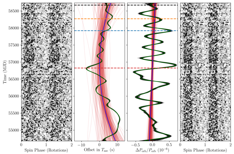
Figure 1: Results from gamma-ray timing analysis. Left panel: photon phases after folding with the original discovery ephemeris (with a constant orbital period). The intensity of each point represents the corresponding probability weight for that photon. The apparent loss of signal around MJDs 55500 and 56800 is due to the varying orbital period. Although present throughout the entire data set, the deviations between the true orbital phase and that predicted by the constant-orbital-period folding model are at their largest at these epochs. Centre left panel: offset in the time of the pulsar’s ascending node from the initial constant orbital period ephemeris. In the timing procedure we fit for an “average” orbital phase, period and first frequency derivative, and model the orbital phase variations as a Gaussian process on top of this base model. Variations requiring a Gaussian process with a larger amplitude or more complexity suffer a Bayesian penalty factor. Black and red lines show the best-fitting orbital phase variations and the underlying “average” orbital model, respectively, for randomly selected samples from the MCMC process. Green and blue curves show the samples with the highest log marginal likelihood. The epochs of our optical observations are marked by horizontal dashed lines with the same colour as the corresponding light curves in Section 4. Centre right panel: as before but for the orbital period (i.e. derivatives of the curves in the previous panel). Right panel: photon phases after correcting for the orbital phase variations using the best-fitting parameter values.

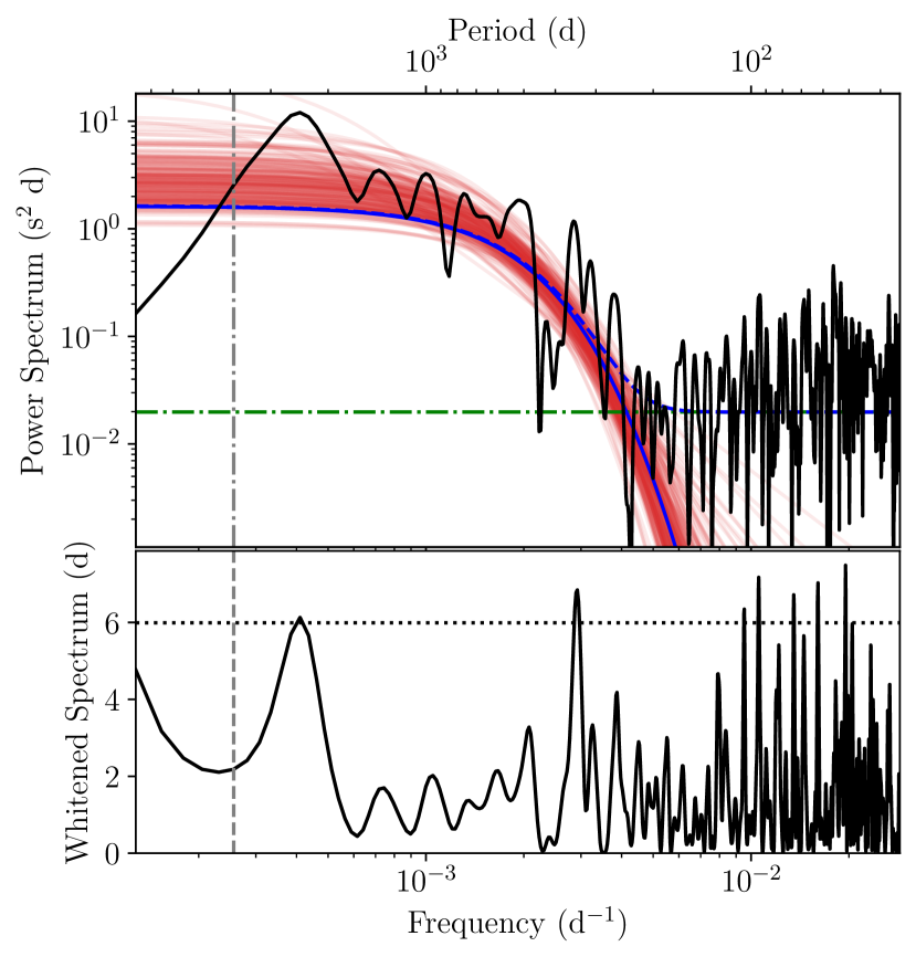
Figure 2: Power spectral density of the orbital phase noise process. The top panel shows the power spectral densities for the orbital phase variations. The green horizontal dot-dashed line shows the estimated measurement uncertainty level, to which the power spectrum breaks at high frequencies. The solid blue and red curves show the best-fitting Matérn covariance function model, and those of random samples from the MCMC process, respectively. The dashed blue line additionally includes the measurement noise level. The lower panels show the power spectra of the orbital phase residuals after whitening using the Cholesky decomposition of the model covariance matrix (i.e. accounting for the blue curve in the upper panel). The horizontal dotted line shows the estimated level which the noise power in $95$% of independent trials should be below. The vertical line in both panels shows the time span covered by the Fermi-LAT data – noise power close to and below this frequency is suppressed by our inclusion of a single orbital period derivative in the timing model.

3.3 Gamma-ray Variability

The subset of transitional redback systems has been seen to transition to and from long-lasting accretion-powered states, in which their gamma-ray flux is significantly enhanced (Stappers et al., 2014; Johnson et al., 2015; Torres et al., 2017). To check for such behaviour from J2039, we investigated potential gamma-ray variability over the course of the Fermi-LAT data span. In 4FGL, J2039 has two-month and one-year variability indices (chi-squared variability tests applied to the gamma-ray flux measured in discrete time intervals) of $44$ with $48$ degrees of freedom, and $13$ with $7$ degrees of freedom, respectively. Although the 1-year variability index is slightly higher than expected for a steady source, we note that the gamma-ray light curves in Ng et al. (2018) indicate that a flare from a nearby variable blazar candidate, 4FGL J2052.2$-$5533, may have contaminated the estimated flux from J2039 around MJD 57100. The true variability is therefore likely lower than suggested by the slightly elevated annual variability index, and indeed the two-month variability index is consistent with a non-variable source.

We also checked for a potential gamma-ray eclipse, which may occur if the binary inclination angle is high enough that the pulsar passes behind the companion star around superior conjunction, as has been observed in the transitional MSP candidate 4FGL J0427.8$-$6704 (Strader et al., 2016; Kennedy et al., 2020). For J2039, this would occur for inclinations $i\gtrsim 78\degr$, and could last for up to $7$% of an orbital period, assuming a Roche-lobe filling companion. We modelled the eclipse as a simple “top-hat” function, in which the flux drops to zero within the eclipse, and used the methods described by Kerr (2019), and applied to the eclipse of 4FGL J0427.8$-$6704 by Kennedy et al. (2020), to evaluate the log-likelihood of this model given the observed photon orbital phases. We find that an eclipse lasting longer than $0.1$% of an orbit is ruled out by the gamma-ray data with $95$% confidence. We interpret this as evidence that the pulsar is not eclipsed, and will use this to constrain the binary inclination while modelling the optical light curves in Section 4.2.

3.3.1 Gamma-ray Orbital Modulation

As noted previously, Ng et al. (2018) discovered an orbitally modulated component in the gamma-ray flux from 4FGL J2039.5$-$5617. Using the now precisely determined gamma-ray timing ephemeris (see Section 3.2) we computed the orbital Fourier power of the weighted photon arrival times, finding $P=29.7$ for a slightly more significant single-trial false-alarm probability of $p_{\rm FA}=\textrm{e}^{-P/2}\approx 4\times 10^{-7}$ compared to that found by Ng et al. (2018). Those authors found the modulation was not detected after MJD 57040 and speculated that this could be due to changes in the relative strengths of the pulsar wind and companion wind/magnetosphere. We do see a slight leveling-off in the rate of increase of $P$ with time; however it picks up again after MJD 58100. Variations in the slope of this function due to statistical (Poisson) fluctuations can appear large when the overall detection significance is low (Smith et al., 2019), and so we do not consider this to be compelling evidence for long-term flux variability from the system.

The gamma-ray and X-ray orbital light curves are shown in Figure 3. We also find no power at higher harmonics of the orbital period, indicating an essentially sinusoidal profile. The gamma-ray flux peaks at orbital phase $\Phi=0.25\pm 0.03$ (pulsar superior conjunction), almost exactly half an orbit away from the X-ray peak, and has an energy-averaged pulsed fraction of $24\pm 5$% (using the definition from Equation (14) of Clark et al., 2017). As noted by Ng et al. (2018), this phasing might suggest an inverse Compton scattering (ICS) origin, as opposed to being the high-energy tail of the population responsible for X-ray synchrotron emission from the intra-binary shock, for example, which would be phase-aligned with the X-ray modulation.

To further investigate this modulation, we performed a second spectral analysis, using the same procedure as above, but additionally separating the photons into “maximum” ($0.0<\Phi\leq 0.5$) and “minimum” ($0.5<\Phi_{\rm orb}\leq 1.0$) orbital phases. We fit the spectral parameters of J2039 separately in each component, while the parameters of other nearby sources and of the diffuse background were not allowed to vary between the two components. The results are given in Table 2 and the resulting spectral energy distributions shown in Figure 4. Subtracting the “minimum” spectrum from the “maximum” spectrum, we find an additional component peaking at around $1\,$GeV, and decaying quickly above that, whose total energy flux is around $30$% of the flux at the orbital minimum. This model has a significant log-likelihood increase of $\Delta\log L=14$ (${\rm TS}=28$ for a false-alarm probability of $5\times 10^{-6}$ given 3 degrees of freedom) compared to our earlier model where the gamma-ray flux is constant with orbital phase.

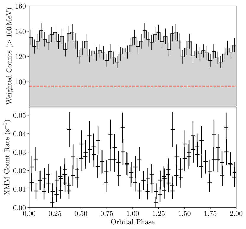
Figure 3: Orbital light curves of J2039 from XMM-Newton (lower panel) and Fermi-LAT (upper panel) observations. Data have been folded using the pulsar timing ephemeris from Section 3.2. The dashed red horizontal line on the gamma-ray light curve indicates the expected background level computed from the distribution of photon weights.

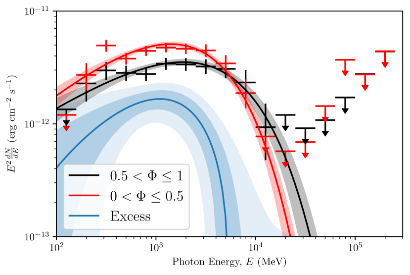
Figure 4: Gamma-ray spectral energy distributions (SEDs) for PSR J2039$-$5617, measured in two discrete orbital phase ranges around pulsar superior ($0.0<\Phi\leq 0.5$) and inferior ($0.5<\Phi\leq 1.0$) conjunctions. Error bars are derived by fitting the normalisation of a power-law spectrum with index $2$ to the flux measured in five discrete logarithmically spaced energy bands per decade. The deviating points at low energies are likely due to source confusion, as seen in the SEDs of several sources in 4FGL. The curved lines and shaded regions illustrate the best-fitting spectral models and one-sigma uncertainties in each phase interval. The blue curve and shaded regions show the difference between the spectral models measured in the two phase intervals.

Table 2: Gamma-ray spectral parameters in two orbital phase regions. Photon and energy fluxes are integrated over photon energies $E>100$ MeV. Uncertainties are at the $1\sigma$ level.

Parameter	$0<\Phi\leq 0.5$	$0.5<\Phi\leq 1$
Photon index, $\Gamma$	$1.25\pm 0.13$	$1.42\pm 0.14$
Exponential factor, $a$ ($10^{-3}$)	$9.0\pm 1.3$	$5.7\pm 1.2$
Photon flux ($10^{-8}$ cm-2 s-1)	$1.8\pm 0.2$	$1.3\pm 0.2$
Energy flux, $G_{\gamma}$ ($10^{-11}$ erg cm-2 s-1)	$1.7\pm 0.1$	$1.3\pm 0.1$

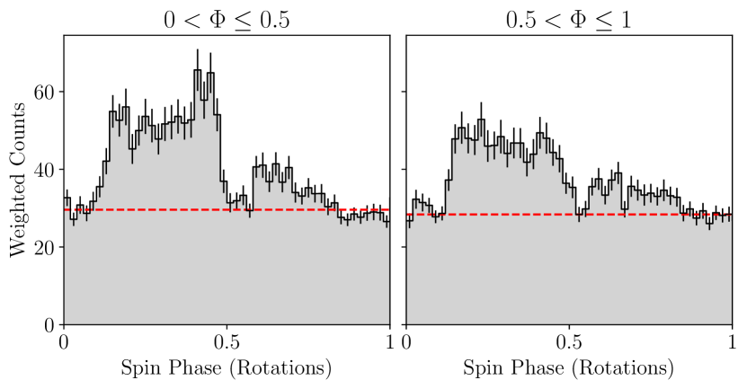
Figure 5: The gamma-ray pulse profile of PSR J2039$-$5617 measured in data taken in two equally-sized orbital phase regions around the pulsar superior (left) and inferior (right) conjunctions. The red dashed line indicates the background level, estimated independently in each orbital phase region using the distribution of photon probability weights. The gamma-ray pulse profile is clearly enhanced around superior conjunction, and there is no evidence for an unpulsed component in either orbital phase region.

Similar orbital modulation has been observed from a handful of other spider systems (Wu et al., 2012; An et al., 2017; An et al., 2018; An et al., 2020). In two of these systems the gamma-ray flux peaks at the same orbital phase as is seen here from J2039, and importantly, from the redback PSR J2339$-$0533 the orbitally modulated component appears to be pulsed in phase with the “normal” intrinsic gamma-ray pulses.

Using the timing solution from Section 3.2, we can now investigate any rotational phase dependence of the orbitally-modulated component. In Figure 5 we show the gamma-ray pulse profile, split into two equal orbital phase regions around the pulsar superior ($0<\Phi\leq 0.5$) and inferior conjunctions ($0.5<\Phi\leq 1$). We find that the estimated background levels, calculated independently in each phase region from the photon weights as $b=\sum_{j}w_{j}-w_{j}^{2}$ (Abdo et al., 2013), are very similar between the two orbital phase selections, that the pulse profile drops to the background level in both, and that the gamma-ray pulse is significantly brighter around the pulsar superior conjunction. There is therefore no evidence for an unpulsed component to the gamma-ray flux from J2039, and the extra flux at the companion inferior conjunction is in fact pulsed and in phase with the pulsar’s intrinsic pulsed gamma-ray emission.

We consider two possible explanations for this orbitally-modulated excess. In these models, charged particles are accelerated in an inclined, fan-like current sheet at the magnetic equator that rotates with the pulsar. The intrinsic pulsed gamma-ray emission is curvature radiation seen when the current sheet crosses the line of sight. In the first scenario, the additional component is ICS from relativistic leptons upscattering the optical photon field surrounding the companion star. In the second, these leptons emit synchrotron radiation in the companion’s magnetosphere. These processes cause the normally unseen flux of relativistic leptons that is beamed towards the observer when the current sheet crosses the line of sight to become detectable as an additional pulsed gamma-ray flux that is coherent in phase with the intrinsic emission. We shall defer a full treatment of this additional emission component to a future work (Voisin, G. et al. 2020, in prep), and instead discuss some broad implications of the detection.

In the ICS scenario, it appears unlikely that the ICS population and the population responsible for the intrinsic (curvature) emission share the same energy. Indeed, the typical energy of the scattered photons, about $E_{s}\sim 1$ GeV, suggests scattering in the Thomson regime (for leptons) with $E_{s}\sim\gamma_{s}^{2}E_{b}$, where $\gamma_{s}$ is the typical Lorentz factor of the scatterer and $E_{b}\sim 1$eV is the energy of soft photons coming from the companion star. This implies $\gamma_{s}\sim 3\times 10^{4}$ which fulfils the condition $E_{s}\ll\gamma_{s}mc^{2}$ necessary for Thomson regime scattering. On the other hand, the Lorentz factor required to produce intrinsic gamma rays at an energy $E_{i}\sim 2$ GeV is about $\gamma_{i}\sim 10^{7}$ assuming the mechanism is curvature radiation (as is favoured by Kalapotharakos et al., 2019). We assumed a curvature radius equal to the light-cylinder radius $r_{\mathrm{LC}}=126\,$km and a magnetic field intensity equal to $B_{\mathrm{LC}}=7\times 10^{4}\,$G in these estimates. Thus, the ICS scenario requires two energetically distinct populations of leptons in order to explain the orbital enhancement. Under this interpretation, the more relativistic curvature-emitting population would also produce an ICS component peaking around 10 TeV, which may be detectable by future ground-based Cherenkov telescopes.

The synchrotron scenario, on the other hand, allows for the possibility that the same particle population responsible for intrinsic pulsed gamma-ray (curvature) emission can produce the orbital flux enhancement, provided the companion magnetic field strength is on the order of $10^{3}$ G (Wadiasingh et al., 2018). The synchrotron critical frequency in a $10^{3}$ G field of the companion magnetosphere is $\sim 1$ GeV for a Lorentz factor of $\gamma_{i}=10^{7}$, while the cooling timescale is about $10^{-5}$ – $10^{-4}$ s, i.e. leptons cool almost immediately after crossing the shock, and phase coherence can be maintained. Moreover, the particles are energetic enough to traverse the shock without being greatly influenced, and would emit in less than a single gyroperiod, so emission would likely be beamed in the same direction as the intrinsic curvature radiation.

For the pulsed orbital modulation in PSR J2339$-$0533, An et al. (2020) also consider an alternative scenario in which intrinsic pulsed emission is absorbed around the pulsar’s inferior conjunction. This model explains the softer spectrum around the maximum, as leptons in the pulsar wind have a higher scattering cross section for low-energy gamma rays. However, they conclude that the pair density within the pulsar wind is far too low to provide sufficient optical depth.

4 Optical observations and Modelling

4.1 New optical observations

We performed optical photometry of J2039 with the high-speed triple-beam CCD camera ULTRACAM (Dhillon et al., 2007) on the NTT on 2017 June 18, 2018 June 02 and 2019 July 07. The first two observations each covered just over one full orbital period, while the third was affected by intermittent cloud cover throughout before being interrupted by thick clouds after 70% of an orbit had been observed. We observed simultaneously in $u_{s},g_{s}$ and $i_{s}$, with 13 s exposures (65 s in $u_{s}$) and negligible dead time between frames. Each image was calibrated using a bias frame taken on the same night and a flat-field frame taken during the same observing run.

All reduction and calibration was performed using the ULTRACAM software pipeline (GROND images were first converted to the ULTRACAM pipeline’s data format). Instrumental magnitudes were extracted using aperture photometry, with each star’s local per-pixel background count rate being estimated from a surrounding annulus and subtracted from the target aperture.

To calibrate the photometry, we took ULTRACAM observations of two Southern SDSS standard fields (Smith, J.A., et al. 2007, AJ, submitted) on 2018 June 01 and 2018 June 04. The resulting zeropoints were used to calibrate the ULTRACAM observations of J2039. Zeropoint offsets between 2017, 2018 and 2019 observations and frame-to-frame transparency variations were corrected via “ensemble photometry” (Honeycutt, 1992) using a set of 15 stars that were present in all ULTRACAM and GROND images of J2039.

To calibrate the archival GROND data, we computed average magnitudes for 5 comparison stars that were covered in $g_{s}$ and $i_{s}$ by the ULTRACAM observations, and fit for a linear colour term between the GROND and ULTRACAM filter sets. Neither $r^{\prime}$ nor $z^{\prime}$ were covered by ULTRACAM. In $r^{\prime}$ we therefore used magnitudes of 4 stars from the APASS catalogue (Henden et al., 2018). No catalogues contained calibrated $z^{\prime}$ magnitudes for stars within the GROND images. We therefore adopted the reference GROND zeropoint in this band. The $g^{\prime}$, $r^{\prime}$ and $i^{\prime}$ the GROND calibrations agreed with these reference zeropoints to within $0.07$ mag. As a cross-check we derived alternative zeropoints using a set of stars in the images which have magnitudes listed in the APASS catalogue. For both GROND and ULTRACAM the APASS-derived zeropoints agree with the calibrations using the ULTRACAM standard-derived zeropoints to within $0.06$ mag in both $g_{s}$ and $i_{s}$.

The resulting light curves in the $g_{s}$ and $i_{s}$ bands (the only two bands covered by all 4 observations) are shown in Figure 6. The long-term changes in the light curve are clearly visible, with $\sim 0.2$ mag variability in the second maximum (near the companion star’s descending node) and $\sim 0.1$ mag variations in the minimum at the companion’s inferior conjunction. The apparent variations around the first maximum (companion’s ascending node), are closer to our systematic uncertainty in the relative flux calibrations.

To estimate the level of variability that can be attributed to our flux calibration, we checked the recovered mean magnitudes of the ensemble stars used to flux-calibrate the data. These all varied by less than $0.05$ mag across all sets of observations.

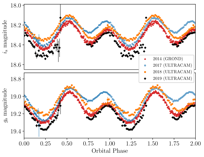
Figure 6: Folded orbital light curves of J2039 across four observing runs (2014 August 16–18 with GROND, 2017 June 18, 2018 June 02 and 2019 July 07 with ULTRACAM). For clarity, the ULTRACAM data points have been combined into $250$ s integrations. The folded light curves are repeated twice, with uncertainties shown only in the first cycle. These are mostly smaller than the corresponding markers. Here, and throughout this paper, orbital phase zero corresponds to the pulsar’s ascending node. The GROND light curves have been corrected to the ULTRACAM magnitude system via colour corrections computed from the magnitudes of comparison stars in the field.

4.2 Light curve modelling

To estimate physical properties of the binary system, we fit a model of the binary system to the observed light curves using the Icarus binary light curve synthesis software (Breton et al., 2012).

Icarus assumes point masses at the location of the pulsar (with mass $M_{\rm psr}$) and companion star centre-of-masses, and solves for the size and shape of the companion star’s Roche lobe, according to an assumed binary mass ratio $q\equiv M_{\rm psr}/M_{\rm c}$, inclination angle $i$, projected velocity semi-amplitude $K_{\rm c}$ and orbital period $P_{\rm orb}$. These parameters are linked through the binary mass function,

$$f(M_{\rm psr})=\frac{M_{\rm psr}\sin^{3}i}{(1+1/q)^{2}}=\frac{K_{\rm c}^{3}P_{\rm orb}}{2\pi\textrm{G}}\,,$$ (6)

and hence only 4 out of these 5 values are independent. With the pulsation detection, we have an extremely precise timing measurement of $P_{\rm orb}$, and the pulsar’s projected semi-major axis ($x$), which further fixes $q=K_{\rm c}P_{\rm orb}/2\pi x$. We therefore chose to fit for $i$ and $K_{\rm c}$, and derive $q$ and $M_{\rm psr}$ from these. For $i$, we adopted a prior that is uniform in $\cos i$ (to ensure that the prior distribution for the orbital angular momentum direction is uniform over the sphere). Since no evidence is seen for a gamma-ray eclipse (see Section 3.3), we assume that the pulsar is not occluded by the companion star, which provides an upper limit on the inclination of $i\lesssim 79\degr$ (the precise limit additionally depends on the size of the star, and was computed “on-the-fly” by Icarus while fitting). We additionally assumed a conservative lower limit of $i>40\degr$, since lower inclinations would require an unrealistically high pulsar mass ($>4\,M_{\odot}$).

The size and shape of the star within the Roche lobe is parameterised by the Roche lobe filling factor $f_{\rm RL}$, defined as the ratio between the radius from the star’s centre-of-mass in the direction towards the pulsar and the distance between the star’s centre-of-mass and the Lagrange L1 point.

Once the shape of the star has been calculated, the surface temperature of the companion star is defined by another set of parameters. The temperature model starts with the “night” side temperature of the star, $T_{\rm n}$, which is the base temperature at the pole of the star prior to irradiation. We assumed a Gaussian prior on $T_{\rm n}$ with mean $5423$ K and width $\pm 249$ K taken from the Gaia colour–temperature relation (Jordi et al., 2010). To account for gravity darkening, we modify the surface temperature at a given location for the local effective gravitational acceleration by $T_{\rm g}=T_{\rm n}(g/g_{\rm pole})^{\beta}$, where $g_{\rm pole}$ is the effective gravitational acceleration at the pole. We used a fixed value of $\beta=0.08$, which assumes that the companion star has a convective envelope (Lucy, 1967).

We account for the effect of heating from the pulsar by modelling it as an isotropically emitting point source of heating flux, with luminosity $L_{\rm irr}$ (although note that the pulsar’s beam is generally more concentrated towards the equator, see Draghis et al. 2019 who account for this when fitting black-widow light curves). In Icarus, heating is parameterised by the “irradiation temperature” $T_{\rm irr}=L_{\rm irr}/(4\pi\sigma A^{2})$, where $\sigma$ is the Stefan-Boltzmann constant and $A=x(1+q)/\sin i$ is the orbital separation. In the later discussion, we will compare this luminosity with the pulsar’s total spin-down power via the heating efficiency, $\epsilon=L_{\rm irr}/\dot{E}$ (Breton et al., 2013) which absorbs several unknown quantities such as the stellar albedo, and the “beaming factor” accounting for the pulsar’s non-isotropic emission. A location on the stellar surface which is a distance $r$ from the pulsar, and whose normal vector is at an angle $\chi$ from the vector pointing to the pulsar, receives heating power of $\sigma T_{\rm irr}^{4}\cos\chi A^{2}/r^{2}$ per unit area. We assume that the star remains in thermal equilibrium, and so this flux is entirely re-radiated, and hence the surface temperature at this location is raised to $T=(T_{\rm g}^{4}+\cos\chi T_{\rm irr}^{4}A^{2}/r^{2})^{1/4}$. To account for the light curve asymmetry and variability, we require additional parameters describing deviations from this direct-heating temperature model; these will be discussed below.

Given this set of parameters, Icarus computes model light curves in each band by solving for the stellar equipotential surface, generating a grid of elements covering this surface, calculating the temperature of each element as above, and simulating the projected flux (including limb darkening) from every surface element at a given inclination angle and at the required orbital phases. For the flux simulation, we used the model spectra from the Göttingen Spectral Library (Husser et al., 2013) produced by the PHOENIX (Hauschildt et al., 1999) stellar atmosphere code. We integrated these model spectra over the transmission curves of the observing setups to obtain flux models in the ULTRACAM and GROND filters.

The flux was rescaled in each band for a distance $d$ and reddening due to interstellar extinction, parameterised by the V-band extinction, $A_{\rm V}$, for which we assumed a uniform prior between $0.0<A_{\rm V}<0.14$, with the (conservative) upper limit being twice that found by Romani (2015) from fits to the X-ray spectrum. Since the Gaia parallax measurement is marginal, we followed the recommendations of Luri et al. (2018) to derive a probability distribution for the distance by multiplying the Gaussian likelihood of the parallax measurement, $p(\varpi|d)$, by an astrophysically motivated distance prior for MSPs. For this, we take the density of the Galactic MSP population along the line of sight to J2039 according to the model of Levin et al. (2013). This model has a Gaussian profile in radial distance from the Galactic centre ($r$) with width $r_{0}=4.5$ kpc, and an exponential decay with height $z$ above the Galactic plane, with scale height $z_{0}=0.5$ kpc. The transverse velocity distribution for binary MSPs in the ATNF Pulsar Catalogue (Manchester et al., 2005) is well approximated by an exponential distribution with mean $v_{0}=100$ km s^-1, which we apply as an additional distance prior. In total, the distance prior is,

$$p(d)\propto p(\varpi\,|\,d)\,d^{2}\,\exp\left[-\frac{v(d)}{v_{0}}-\frac{z(d)}{z_{0}}-\frac{1}{2}\left(\frac{r(d)}{r_{0}}\right)^{2}\right]\;,$$ (7)

where the $d^{2}$ term arises from integrating the Galactic MSP density model at each distance over the 2D area defined by the Gaia localization region. Finally, we used the radio dispersion measure, $\textrm{DM}=24.6$ pc cm^-3 (see Paper II) as an additional distance constraint. The Galactic electron density model of Yao et al. (2017, hereafter YMW16) gives an estimated distance of $d=1.7$ kpc, with nominal fractional uncertainties of $\pm 45$%. We therefore multiplied the distance prior by a log-normal distribution with this mean value and width. This overall prior gives a 95% confidence interval of $1.2\,\textrm{kpc}<d<3.0\,\textrm{kpc}$, with expectation value $\hat{d}=1.9$ kpc.

In our preliminary Icarus models, constructed prior to the spectroscopic observations by Strader et al. (2019) and the pulsation detection presented here, we jointly fit all three light curves, and additionally fit for $P_{\rm orb}$ and $T_{\rm asc}$. For this we used a Gaussian prior on $P_{\rm orb}$ according to the best-fitting period and uncertainty from the Catalina Surveys Southern periodic variable star catalogue (Drake et al., 2017, see Section 2), and refolded the optical observations appropriately. The resulting posterior distributions on $P_{\rm orb}$, $T_{\rm asc}$ and on $x$ were used to constrain the parameter space for the gamma-ray pulsation search in Section 3.1.

In these preliminary models, we accounted for the light curve asymmetry and variability by describing the surface temperature of the star using an empirical spherical harmonic decomposition whose coefficients could vary between the three epochs. While this model served our initial goal of phase-aligning the light curves to constrain the orbital parameters, the spherical harmonic temperature parameterisation suffered from several deficiencies. Firstly, the decomposition had to include at least the quadrupole ($l=2$) order to obtain a satisfactory fit. Several of these coefficients were highly correlated with one another, and polar terms $(m=0)$ are poorly constrained as the system is only viewed from one inclination angle, leading to very poor sampling efficiency. Secondly, the quadrupole term naturally adds power into the second harmonic of the light curve, changing the amplitude of the two peaks in the light curve. In the base model, this amplitude depends only on the inclination and Roche-lobe filling factor, and so the extra contribution of the quadrupole term made these parameters highly uncertain.

To try to obtain more realistic parameter estimates, we instead modelled the asymmetry and variability by adding a cold spot to the surface temperature of the star. While cool star spots caused by magnetic activity are a plausible explanation for variability and asymmetry in the optical light curves (van Staden & Antoniadis, 2016), other mechanisms such as asymmetric heating from the pulsar (Romani & Sanchez, 2016; Sanchez & Romani, 2017), or heat re-distribution due to convective flows on the stellar surface (Kandel & Romani, 2020; Voisin et al., 2020c), may also explain this. Our choice to model the light curves using a cool spot came from this being a convenient parameterisation for a temperature variation on the surface of the star, rather than from assuming that variability is due to magnetic star spot activity.

In our model, this spot subtracts from the gravity-darkened temperature of the star, with a temperature difference of $\tau$ at the centre of the spot, which falls off with a 2D Gaussian profile with width parameter $\rho$ in angular distance ($\Delta$) from the centre of the spot. The spot location on the surface of the star is parameterised by the polar coordinates $(\theta,\phi)$, with $\theta=0$ aligned with the orbital angular momentum, $\phi=0$ pointing towards the pulsar and $\phi=90\degr$ aligned with the companion’s direction of motion. We assumed a sinusoidal prior on $\theta$ to ensure our priors covered the surface of the star approximately uniformly (the approximation would be exact for a spherical, i.e. non-rotating and non-tidally distorted star). The spot width was confined to be $5\degr<\rho<30\degr$. The lower limit prevents very small and very cold spots, while the upper limit ensures that the effects of spots do not extend over much more than one hemisphere.

To prevent over-fitting, we added an extra penalty factor on the total (bolometric) difference in flux that the spot adds to the model. This is, approximately, proportional to $I=\iint_{S}\,\tau^{4}e^{-(\Delta(\theta,\phi)^{2}/2\rho^{2})}\,dS$ where $S$ is the surface of the star. In our fits we adopted a Gaussian prior on $I$, centred on $I=0$ with width parameter $\sigma_{I}=6.25\times 10^{10}\,\textrm{K}^{4}\,\textrm{sr}$, corresponding to a $-500$K spot covering 1 steradian of the star’s surface. Noting from Figure 6 that the first peak (at the pulsar’s ascending node) is always larger than the second, and that the variability seems to be strongest around the second peak, we assumed in our model that the light curve asymmetry is due to a variable cold spot ($\tau<0$ K) on the leading edge of the companion star, and confined $0\degr<\phi<180\degr$.

To investigate the light curve variability and understand what effect this has on our inference of the binary parameters, we chose to fit each light curve separately. Here we only model the three complete light curves from 2014, 2017 and 2018. The partial 2019 light curve is missing the first peak, and hence models fit only to the data around the variable second peak would have very high uncertainties on the fit parameters, making this of limited use compared to the other three light curves. We included the ULTRACAM $u_{s}$ data in our model fitting, since they were obtained simultaneously with the $i_{s}$ and $g_{s}$ data without requiring additional observing time, and provide an additional colour for temperature estimation. However, as the signal-to-noise is much lower in this band, we do not expect it to have had a large effect on the results.

To account for uncertainties in our atmosphere models, extinction, or photometric calibration, we allowed for constant offsets in the magnitudes in each band, penalising the chi-squared log-likelihoods using a Gaussian prior on the magnitude offset with a width of $0.05$ mag. As the resulting reduced chi-squared was greater than unity, we also applied rescaling factors to the uncertainties in each band. Both the band calibration offsets and uncertainty rescaling factors were computed to maximise the penalised log-likelihood.

At each sampled location in the parameter space, Icarus additionally computed the projected velocity of every surface element, and averaged these weighting by their $r^{\prime}$ flux, to obtain a simulated radial velocity curve. This filter band was chosen as it covers the sodium absorption line seen in Strader et al. (2019). The simulated radial velocity curve was compared to the measured radial velocities from Strader et al. (2019), additionally fitting for a constant systemic radial velocity, and the resulting chi-squared term added to the overall log-likelihood.

The model fits were performed using the pymultinest Python interface (Buchner et al., 2014) to the Multinest nested sampling algorithm (Feroz et al., 2013). The best fitting models and light curves are shown in Figure 7, the posterior distributions for our model parameters are shown in Figures 8, 9 and 10, and numerical results are given in Table 3. While the inferred posterior distributions from each epoch generally overlap with each other (except for the spot and heating parameters encapsulating variability), in the following discussion we take the full range covered by the 95% confidence intervals of the three posterior distributions as estimates for the model uncertainty, in the hope that biases due to variability are contained within that range.

Table 3: Icarus fit results. Numerical values are the median of the marginalised posterior distributions output by Multinest, with the $95$% confidence regions shown in sub- and superscript.

Parameter	2014 June 16–18 (GROND)	2017 June 18 (ULTRACAM)	2018 June 02 (ULTRACAM)
$\chi^{2}$ (degrees of freedom)	$958.6\,(824)$	$3930.3\,(3529)$	$3699.5\,(3330)$
Icarus fit parameters
Systemic velocity (km s-1)	$6_{-6.5}^{+6.6}$	$5.9_{-6.4}^{+6.4}$	$6.4_{-6.6}^{+6.7}$
Companion’s projected radial velocity, $K_{\rm c}$ (km s-1)	$327.3_{-8.8}^{+8.9}$	$329.6_{-8.7}^{+8.6}$	$325.4_{-8.9}^{+9}$
Distance, $d$ (kpc)	$1.7_{-0.14}^{+0.16}$	$1.69_{-0.11}^{+0.12}$	$1.8_{-0.17}^{+0.21}$
V-band extinction, $A_{V}$	$0.072_{-0.069}^{+0.064}$	$0.091_{-0.082}^{+0.047}$	$0.095_{-0.086}^{+0.043}$
Inclination, $i$ ($\degr$)	$74.5_{-5.1}^{+3.7}$	$77.1_{-3.8}^{+1.2}$	$69_{-8}^{+8.8}$
Roche-lobe filling factor, $f_{\rm RL}$	$0.835_{-0.014}^{+0.021}$	$0.821_{-0.008}^{+0.012}$	$0.839_{-0.033}^{+0.048}$
Base temperature, $T_{\rm n}$ (K)	$5451_{-57}^{+82}$	$5395_{-74}^{+87}$	$5471_{-109}^{+124}$
Irradiating temperature, $T_{\rm irr}$ (K)	$3456_{-72}^{+96}$	$3807_{-85}^{+94}$	$3700_{-141}^{+160}$
Spot central temperature difference, $\tau$ (K)	$-540_{-150}^{+170}$	$-620_{-260}^{+340}$	$-600_{-80}^{+70}$
Spot Gaussian width parameter, $\rho$ ($\degr$)	$23_{-3.9}^{+5.7}$	$14.4_{-3.7}^{+10.9}$	$28_{-3.9}^{+1.9}$
Spot co-latitude, $\theta$ ($\degr$)	$42.7_{-7.5}^{+9.1}$	$33.1_{-10.5}^{+16.1}$	$96.7_{-13.1}^{+13.2}$
Spot longitude, $\phi$ ($\degr$)	$77.9_{-4.6}^{+3}$	$73.6_{-12.4}^{+6.2}$	$56.3_{-4.6}^{+3.8}$
Derived parameters
Heating efficiency, $\epsilon$	$0.061_{-0.007}^{+0.011}$	$0.089_{-0.01}^{+0.012}$	$0.086_{-0.019}^{+0.03}$
Pulsar mass, $M_{\rm psr}$ ($M_{\odot}$)	$1.2_{-0.11}^{+0.14}$	$1.18_{-0.09}^{+0.1}$	$1.3_{-0.2}^{+0.31}$
Companion mass, $M_{\rm c}$ ($M_{\odot}$)	$0.165_{-0.012}^{+0.017}$	$0.162_{-0.008}^{+0.011}$	$0.18_{-0.026}^{+0.041}$
Mass ratio, $q\equiv M_{\rm psr}/M_{\rm c}$	$7.27_{-0.2}^{+0.2}$	$7.32_{-0.19}^{+0.19}$	$7.22_{-0.2}^{+0.2}$
Volume-averaged companion density (g cm-3)	$4.38_{-0.14}^{+0.1}$	$4.48_{-0.09}^{+0.07}$	$4.35_{-0.27}^{+0.25}$
Spot integral, $I$ ($10^{10}$ K4 sr)	$8.4_{-5.7}^{+8.8}$	$6.0_{-5.3}^{+9.4}$	$18.1_{-6.5}^{+8.3}$

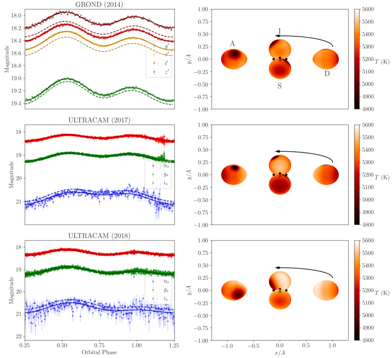
Figure 7: Best-fitting optical light curve models for J2039. Each row shows the best-fitting model for a given epoch. Left panels show the observed light curves and uncertainties (coloured error bars) in each band. The fluxes in each band predicted by the best-fitting Icarus model are shown as dashed curves. When fitting these models we allowed for small offsets in the flux calibration of the observed light curves. The solid curves show the model light curves after applying these calibration offsets. Right panels show the Icarus model according to the best-fitting parameters at the pulsar’s ascending (A) and descending (D) nodes, and superior (S) and inferior (I) conjunctions, marked on the top right panel, with the direction of motion shown by an arrow. The pulsar’s position at each phase is shown by a black dot. Phase zero in the light curves corresponds to the pulsar’s ascending node. The axes are in units of the orbital separation ($A$). The surface temperature of the companion star is shown by the colour bar.

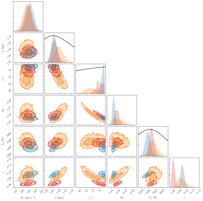
Figure 8: Posterior distributions for the Icarus model parameters. Red, blue and orange histograms and contours show the posterior distributions from fits to the GROND, ULTRACAM (2017) and ULTRACAM (2018) light curves, respectively. Contour lines are shown at $1\sigma$ and $2\sigma$ levels. Where a non-uniform prior is assumed, this is shown as a black curve on the corresponding parameter’s 1-dimensional histogram.

5 Results and Discussion

5.1 Binary Inclination and Component Masses

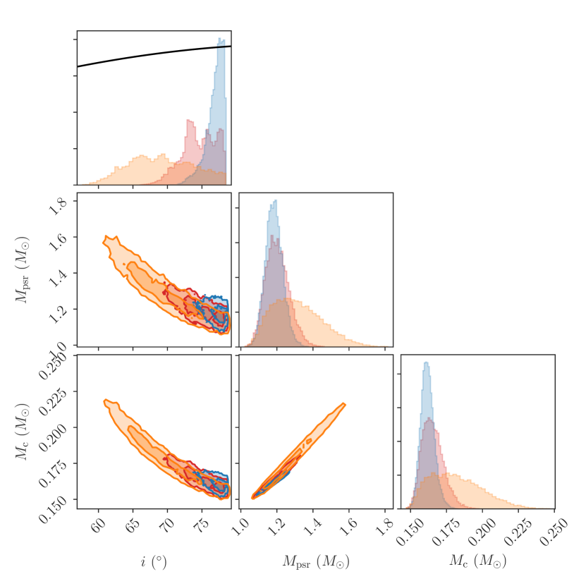
Figure 9: Posterior distributions from Icarus model fitting, as in Figure 8, but for the binary inclination, pulsar and companion masses.

Perhaps one of the more important questions is whether or not we are able to obtain a reliable measurement of the mass of the neutron star in the system. The maximum neutron star mass is a crucial unknown quantity which can discriminate between different nuclear equations-of-state (see Özel & Freire, 2016, and references therein). Recent works (van Kerkwijk et al., 2011; Linares et al., 2018) have found very heavy pulsar masses for spider pulsars, and there are hints that these systems may in general contain heavier neutron stars than e.g. double neutron star systems (Strader et al., 2019).

Combining the radial velocity curve measured via spectroscopy by Strader et al. (2019) with our pulsar timing measurement of the pulsar’s projected semi-major axis constrains the mass ratio to $q=7.3\pm 0.2$. Hence, all parameters in the binary mass function (Equation 6) are relatively well measured, with the exception of the binary inclination angle. Measuring this by modelling the optical light curves was therefore a key goal for our study of this system. The observed asymmetry and variability in the light curve are significant complicating factors for this, as estimates for the inclination angle are determined by the amplitude of the ellipsoidal peaks. In J2039, these do not have equal amplitudes, and vary over time.

Our optical model fits to all three complete orbital light curves consistently preferred high inclinations, hitting the upper limit of ($i\lesssim 79\degr$) imposed by our assertion that the pulsar is not eclipsed at superior conjunction. The second ULTRACAM light curve results in the widest $95$% confidence interval, with $61\degr<i<78\degr$. Marginalising over the uncertainty in the radial velocity amplitude, the corresponding pulsar mass range is $1.1M_{\odot}<M_{\rm psr}<1.6M_{\odot}$, with a median of $M_{\rm psr}\approx 1.3M_{\odot}$, but the models for the other two epochs give narrower ranges $1.1\,M_{\odot}<M_{\rm psr}<1.35\,M_{\odot}$. The posterior distributions on these parameters are shown in Figure 9.

Inclination angles derived from optical light curve fits are highly dependent on the chosen temperature and irradiation models and priors. In particular, we caution that there is likely to be a large (but unknown) systematic uncertainty underlying our inclination estimates, caused by our simplifying assumption that the variability and asymmetry can be modelled by one cold spot on the leading face of the star. Other models for light curve asymmetry, e.g. intra-binary shock heating models or models featuring convective winds on the stellar surface (Romani & Sanchez, 2016; Kandel & Romani, 2020; Voisin et al., 2020c), may give different results. Pulsar masses derived from optical light curve modelling should therefore be treated with caution, as the results can be highly model-dependent. For instance, if part of the asymmetry is caused by excess heating on the trailing face of the star rather than a cool spot on the leading face, then the leading peak of the light curve will be larger than predicted by the direct-heating model, and the model’s inclination angle will increase to compensate. Nevertheless, our results suggest that a high inclination and fairly low pulsar mass is compatible with the observed light curves.

Our resulting mass is rather lower than those inferred from other redback systems, which Strader et al. (2019) found to cluster around $1.8\,M_{\odot}$, but has a range similar to that found for PSR J1723$-$2837 ($M_{\rm psr}<1.4\,M_{\odot}$) by van Staden & Antoniadis (2016). While some of the redback masses compiled by Strader et al. (2019) do have strict lower limits (i.e. for edge-on orbits) that are above our inferred mass range, it is possible that unmodelled asymmetries and variability may be systematically biasing optical-modelling based inclination measurements to lower values, and hence biasing the redback pulsar mass distribution towards higher values.

By generating and fitting a flux-averaged radial velocity curve, our binary system model additionally corrects for possible biases in the observed radial velocity curve due to a difference between the centre of mass of the companion star and the position on the surface where spectral lines contribute most strongly to the observed spectra (e.g., Linares et al., 2018). For J2039, heating has a fairly small effect on the light curve, and the resulting correction to the radial velocity curve is small: the epoch with the largest inferred centre-of-mass radial velocity amplitude (2017 June 18) has $K_{2}=330\pm 5$ km s^-1, compared to $K_{2}=324\pm 5$ km s^-1 that Strader et al. (2019) found from a simple sinusoidal fit. This implies that the required $K_{2}$-correction is only $\Delta K_{2}/K_{2}\lesssim 2$%, and only increases the inferred pulsar mass by $\Delta M_{\rm psr}/M_{\rm psr}\lesssim 6$%. While here this additional bias is far lower than that caused by our uncertainty on the inclination, this is not true in general for other redback systems. Large changes in the heating of redback companions have been observed (Cho et al., 2018), and so reliable centre-of-light corrections require photometry observations to be taken as close in time as possible to spectroscopic radial velocity measurements to mitigate possible errors due to variations in heating.

Our pulsar mass range is lower than that estimated by Strader et al. (2019) ($M_{\rm psr}>1.8M_{\odot}$) from similar fits to the GROND light curve. Prior to our pulsation detection, the binary mass ratio was unconstrained, and so this was an additional free parameter in their model. The authors used two large cold spots in their model, which were both found to lie towards the unheated side of the star. These spots will affect the amplitudes of both ellipsoidal peaks, and therefore will affect the estimation of the inclination angle, filling factor and mass ratio that are constrained by these amplitudes. Their fits found a much lower mass ratio than is obtained from the pulsar’s semi-major axis measurement ($q<5.3$ vs. $q=7.3\pm 0.2$ here) and a nearly Roche-lobe filling companion $f_{\rm RL}\approx 95$%. Both of these parameter differences will increase the amplitude of the ellipsoidal modulations, allowing for a more face-on inclination and thus a heavier pulsar, explaining our disagreement.

The inferred inclination angle is also (qualitatively) consistent with the observed gamma-ray pulse profile. Since the pulsar has been spun-up via accretion its spin axis should be aligned to the orbital axis, and hence the pulsar viewing angle (the angle between the line-of-sight and the pulsar’s spin axis) will match the orbital inclination. The gamma-ray pulse profile features one broad main peak, with a smaller trailing peak. This therefore rules out an equatorial viewing angle to the pulsar, and hence an edge-on orbital inclination $i\sim 90\degr$ as in that case the gamma-ray pulse should exhibit two similar peaks approximately half a rotation apart. The detection of radio pulsations enables a full investigation of this, fitting both the gamma-ray pulse profile shape and its phase relative to the radio pulse using theoretical pulse emission models. This will be described in detail in Paper II, but we note here that these models suggest a lower viewing angle of $i\sim 67\degr$, for a pulsar mass of $M_{\rm psr}\sim 1.4\,M_{\odot}$.

For the companion mass, we find $0.15M_{\odot}<M_{\rm c}<0.22{\rm M}_{\odot}$. Our Icarus model fits gave the companion star base temperature $T_{\rm n}\approx 5400\,$K and volume-averaged radius $R_{\rm c}\approx 0.4$ R_⊙. These are both significantly larger than would be expected for a main-sequence star of the same mass. Indeed, this is not surprising, as the accretion required to recycle the MSP will have stripped the majority of the stellar envelope, while tidal forces and heating from the pulsar continue to add additional energy into the companion star (Applegate & Shaham, 1994), causing a further departure from ordinary stellar evolution.

5.2 Distance and Energetics

The Icarus fits to our three light curves all returned consistent distance estimates around $d=1.7^{+0.3}_{-0.1}$ kpc, consistent with the Gaia parallax and YMW16 DM distance estimates. Assuming a fiducial distance of $d=1.7$ kpc, the Gaia proper motion measurement implies a transverse velocity of $v_{\rm T}\approx 125$ km s^-1. This transverse velocity will induce an apparent linear decrease in both the spin and orbital frequencies due to the increasing radial component of the initially transverse velocity (hereafter referred to as the Shklovskii effect after Shklovskii, 1970). This effect accounts for around $20$% of the observed spin-down rate. An additional contribution to the observed spin-down rate comes from the pulsar’s relative acceleration due to the Galactic rotation and gravitational potential. Using the formula given by Matthews et al. (2016) and references therein, we estimate this accounts for less than 1% of the observed spin-down rate. At the fiducial distance the gamma-ray flux corresponds to a luminosity of $L_{\gamma}=5\times 10^{33}$ erg s^-1, or a Shklovskii-corrected gamma-ray efficiency of $\eta_{\gamma}=L_{\gamma}/\dot{E}=21$%, which is typical for gamma-ray MSPs (Abdo et al., 2013). Recently, Kalapotharakos et al. (2019) discovered a “fundamental plane” linking pulsars’ gamma-ray luminosities to their spin-down powers, magnetic field strengths and spectral cut-off energies (Kalapotharakos et al., 2019). For J2039, this predicts $L_{\gamma,\textrm{FP}}=1.3\times 10^{34}\,\textrm{erg s}^{-1}$, or $0.4\,\textrm{dex}$ above the observed value, consistent with the scatter about the fundamental plane seen by Kalapotharakos et al. (2019).

In our Icarus model, we assume that the inner side of the companion star is heated directly by flux from the pulsar. For PSR J2039$-$5617, our optical models hint that the heating flux reaching the companion star may be variable, and is on the order of a few percent of the total spin-down luminosity of the pulsar, with $\epsilon=L_{\rm irr}/\dot{E}\sim 0.05$ to $0.12$. This is a somewhat lower efficiency than is typically observed in spider systems, where heating normally accounts for around $20$% of the pulsar’s spin-down power (Breton et al., 2013; Draghis et al., 2019).

The precise nature of the mechanism by which redback and black-widow pulsars heat their companions is currently unclear. For J2039, the inferred gamma-ray luminosity is larger than the heating power, and so we may infer that gamma rays are a sufficient heating mechanism in this case. For other spiders, this is not always true, with heating powers found to be much larger than gamma-ray luminosities (e.g., Nieder et al., 2019). Some discrepancy between the two can be explained by underestimated distances, or beamed (i.e. non-isotropic) gamma-ray flux that is preferentially emitted in the equatorial plane, although heating efficiencies and gamma-ray efficiencies remain only loosely correlated even with these corrections (Draghis et al., 2019). This may indicate that another mechanism, e.g. high-energy leptons in the pulsar wind, is responsible for heating the companion star. Note that both $\eta_{\gamma}$ and $\epsilon$ are fractions of $\dot{E}$, so while $\dot{E}$ is an order-of-magnitude estimate dependent on the chosen value for the pulsar moment of inertia, the ratio between $\eta_{\gamma}$ and $\epsilon$ is independent of this.

5.3 Optical light curve asymmetry and variability

In the above heating efficiency calculation, we only included direct heating i.e. flux from the pulsar that is immediately thermalised and re-radiated from the surface of the companion star at the location on which it impinges. For J2039 the asymmetry of the light curve, and relative lack of variability on the leading peak may suggest that some heating is being re-directed toward the trailing face of the companion star, keeping this side at a more constant temperature. However, with only three optical light curves covering this orbital phase this is purely speculative, and requires additional optical monitoring to check for variability in the leading peak.

Nevertheless, similar light curve asymmetry, with the leading peak typically appearing as the brighter of the two, seems to be common in many types of close binary systems (e.g. cataclysmic variables (CVs) and W UMa-type eclipsing binaries), where it is often referred to as the O’Connell effect (after O’Connell, 1951). Several processes have been proposed to explain this in general, and in redbacks in particular, but so far without consensus. Possible processes include: reprocessing of the pulsar wind by a swept-back asymmetric intra-binary shock (Romani & Sanchez, 2016); channeling of charged particles in the pulsar wind onto the poles of a companion’s misaligned dipolar magnetic field (Sanchez & Romani, 2017; Wadiasingh et al., 2018); or heat redistribution due to fluid motion in the outer layers of the star (Martin & Davey, 1995; Kandel & Romani, 2020; Voisin et al., 2020c).

For J2039, the presence of an intra-binary shock wrapping around the pulsar is required to explain the observed orbital modulation of X-rays. Following the model of Romani & Sanchez (2016), it therefore seems plausible that extra heating flux could be directed at the trailing face of the companion star, and could at least partially explain the observed light-curve asymmetry. We are then left to explain the variability in the light curve. Cho et al. (2018) observe similar variability in the light curves of three other redback systems, attributing this to variability in the stellar wind and hence in the intra-binary shock.

An alternative explanation for redback variability is that magnetic activity in the companion leads to large cool star spots on the stellar surface, which migrate around the star and may appear and disappear over time. This star-spot interpretation has been invoked to explain the similar optical variability seen in long-term monitoring of the redback system PSR J1723$-$2837 (van Staden & Antoniadis, 2016). A periodogram analysis of these light curves found a component with a period slightly shorter than the known orbital period, which the authors interpret as being due to asynchronous (i.e. non-tidally locked) rotation of the companion star. Alternatively, this could also be due to differential rotation of the stellar surface, as seen in sun spots, and observed e.g. in CV secondaries via Roche tomography (e.g., Hill et al., 2014). Given the year-long time intervals between our ULTRACAM light curves of J2039 we cannot perform the same analysis to track a single variable component over time to confirm this picture, but this may be possible in the future with sufficient monitoring. Another interesting question that may be addressed with additional monitoring is whether or not the optical variability correlates with the variations in the orbital period, as both may be linked through magnetic cycles in the stellar interior.

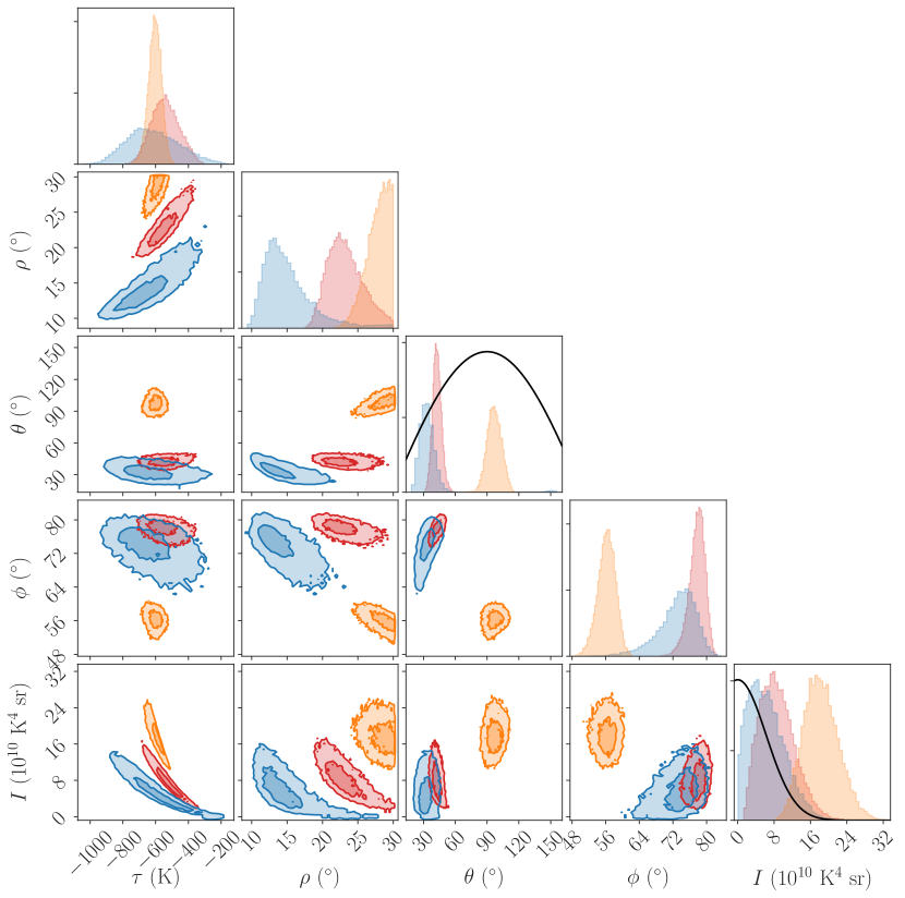
Figure 10: Posterior distributions from Icarus model fitting, as in Figure 8, but for the parameters of the cold spot added to the companion’s surface. These parameters account for the significant variability observed in the light curves, hence the rather different values recovered.

To create our binary system models, we used a toy model for the stellar surface temperature that included a variable cold spot to account for the asymmetry and variability. The posterior distributions on the parameters of these spots are shown in Figure 10. This model is certainly an over-simplification of the truth, and so we will avoid placing much emphasis on the numerical results for these parameters, noting that our goal was instead to marginalise over the variability to retrieve estimates for more tangible quantities such as the inclination and filling factor. Our chosen prior, which aims to minimise the bolometric flux $\propto\tau^{4}\sigma^{2}$ subtracted by the cool spot, penalises small but very cold spots over larger and warmer spots. This prevents our model reaching the very cold spot temperatures ($\tau\sim-2000$ K) that have been observed in well-studied main-sequence stars (Berdyugina, 2005). Instead, our model prefers large spots (close to our upper limit of $\rho=30\degr$) with a central temperature difference between $\tau\sim-300$ K to $\tau\sim-700$ K. While such a temperature reduction could be plausibly explained by magnetic star spot activity, we are hesitant to interpret these as “true” star spots, but rather consider them to be areas of decreased temperature due to unknown variable effects, e.g. asymmetric heating from the pulsar, or heat re-distribution due to convective flows on the stellar surface. Continued photometric monitoring of J2039 to test the star-spot explanation may reveal evidence that these cool areas migrate across the surface of the star, as they do in PSR J1723$-$2837 (van Staden & Antoniadis, 2016). We discuss this possibility further below. Furthermore, a dedicated study of the spectra observed by Strader et al. (2019) may be able to detect the presence of spectral lines associated with cooler temperatures to further investigate the star-spot hypothesis.

We also note that a better understanding of variability in rotationally powered redback systems may offer insight into some of the most extreme behaviour exhibited by binary MSP systems: the sudden (dis)appearance of accretion discs in transitional MSP systems (tMSPs, Archibald et al., 2009; Papitto et al., 2013; Bassa et al., 2014; Stappers et al., 2014). To provide material to power a tMSP’s accretion state, the companion star must be overfilling its Roche lobe. However, optical modelling of PSR J1023$+$0038 somewhat surprisingly suggests a companion that significantly underfills its Roche lobe (McConnell et al., 2015; Shahbaz et al., 2019). This therefore requires a significant change in the radius of the companion star, and the timescale on which this takes place is currently unknown. For J2039, we also find that the companion star is significantly smaller than its Roche lobe ($f_{\rm RL}\approx 0.83$), and do not find any evidence for variations in the stellar radius over the three light curves.

5.4 Orbital Period Variability

In Section 3.2 we measured the orbital period of J2039, finding significant deviations in the orbital phase from a constant-period model. Such variations are common among redback systems (e.g., Deneva et al., 2016; Archibald et al., 2009; Pletsch & Clark, 2015). This phenomenon has been attributed to the Applegate mechanism (Applegate & Patterson, 1987; Applegate & Shaham, 1994), originally invoked to explain period variations in eclipsing Algol-type and CV binaries, in which periodic magnetic activity cycles in the convective zone of the companion star introduce a varying quadrupole moment, which couples with the orbital angular moment to manifest as variations in the orbital period.

Using our new Gaussian process description for the orbital phase variations, we can hope to quantify the required changes in the quadrupole moment using the best-fitting values for the hyperparameters of the Gaussian process used to model the orbital phase variations in Section 3.2.

Under the Applegate model, the change in orbital period is directly related to the change in the companion star’s gravitational quadrupole moment $Q$ (Applegate & Patterson, 1987),

$$\frac{\Delta P_{\rm orb}}{P_{\rm orb}}=-9\frac{\Delta Q}{M_{\rm c}A^{2}}\,,$$ (8)

where $A=x(1+q)/\sin i$ is the orbital separation. For comparison, the total quadrupole moment induced by the spin of the companion star and the tidal distortion in the pulsar’s gravitational field is (Voisin et al., 2020a)

$$\frac{Q}{M_{\rm c}A^{2}}=-\frac{2}{9}k_{2}\left(\frac{R_{\rm c}}{A}\right)^{5}\left(4q+1\right)\,,$$ (9)

where $R_{c}$ is the radius of the companion star and $k_{2}$ is the apsidal motion constant, a parameter describing the deformability of the companion star (Sterne, 1939). For solar-type stars $k_{2}\sim 0.035$ (Ogilvie, 2014), while if we assume that redback companions are akin to the companions in CV systems whose outer envelopes have also been stripped through accretion then we may expect a smaller value $k_{2}\sim 10^{-3}$ (Cisneros-Parra, 1970). For J2039, the hyperparameter $h=3.9^{+2.2}_{-1.2}$ s corresponds to the typical fractional amplitude for the variations in orbital phase. Taking the simpler squared exponential covariance function of Equation (4) corresponding to $n\to\infty$ then the deviations in orbital period have covariance function,

$$\begin{split}K_{\Delta P_{\rm orb}/P_{\rm orb}}(t_{1},t_{2})&=\frac{\partial^{2}K}{\partial t_{1}\partial t_{2}}\\ &=\frac{h^{2}}{l^{2}}\exp\left(-\frac{(t_{1}-t_{2})^{2}}{2\ell^{2}}\right)\left(1-\frac{(t_{1}-t_{2})^{2}}{\ell^{4}}\right)\,.\end{split}$$ (10)

The typical (fractional) amplitude of the orbital period variations is therefore $\Delta P_{\rm orb}/P_{\rm orb}\sim h/\ell=(3\pm 1)\times 10^{-7}$, corresponding to $\Delta Q/Q\sim 3\times 10^{-5}k_{2}^{-1}$. The time-varying component to the gravitational quadrupole moment is therefore required to be of order a few percent of the total expected quadrupole moment at most to explain the observed orbital period variations. From this, it seems plausible that the observed period variations can be powered by quadrupole moment changes, without requiring that a large fraction of the star be involved in the process. The required fractional quadrupole moment changes are very similar to those recently calculated for the companion to the black widow PSR J2051$-$0827 by Voisin et al. (2020b), despite the large difference in their masses.

For our assumed Matérn covariance function, the parameter $n$ is related to how smooth the noise process is: random walks in orbital phase, period or period derivative would manifest as noise processes with $n=1/2,\,3/2$ or $5/2$ respectively (Kerr et al., 2015). This hyperparameter may therefore encode information about the source of the orbital period variation. If the quadrupole moment exhibits random walk behaviour (i.e. the stellar structure switches rapidly between different states), we would expect to see a random walk in orbital period ($n=3/2$). Alternatively, if the system is affected by a variable torque (e.g. variable mass loss, or magnetic braking) then this would manifest as a random walk in the orbital period derivative or higher orders ($n\gtrsim 5/2$).

Unfortunately, Figure 2 illustrates that we are insensitive to the value of $n$, as the variability quickly falls below the measurement uncertainty level for periods shorter than $\ell\approx 130$ d, preventing measurement of the power-law slope above the corner frequency. We find only that a very shallow power-law spectrum $n<1$ is ruled out with $95\%$ confidence, but models with finite $n>1.5$ fit the data equally well as the squared exponential kernel corresponding to $n\to\infty$.

We also find marginal evidence for an excess in the noise power at periods longer than the 11-years of Fermi-LAT data. This is not well accounted for by a longer correlation timescale $\ell$ and shallower spectral index, as this leaves excess power at intermediate frequencies, and we do find that a break in the spectrum is preferred, with $\ell\ll T_{\rm obs}$. One explanation could be that instead of breaking to a constant power level at low frequencies, the noise process breaks to a shallower power law. However, with only a handful of independent frequencies below the corner frequency, this slope is hard to probe, although this may be worth revisiting as the timing baseline grows.

Alternatively, this low-frequency excess could be explained by a steadily increasing orbital period, which would introduce a quadratic term in the orbital phase that would appear as noise power at a period longer than the observation timespan. In Section 3.2, we accounted for this by including a constant orbital period derivative $\dot{P}_{\rm orb}=(8\pm 5)\times 10^{-12}$.

While there are several physical processes which could lead to a long term increase in the orbital period on top of the Applegate-style stochastic variability, the magnitude of the effect here is hard to reconcile. For example, the Shklovskii-induced orbital period derivative is $\dot{P}_{\rm orb,Shk}=v_{\rm T}^{2}P_{\rm orb}/cd=2\times 10^{-14}$, almost three orders of magnitude smaller than the measured value. Other incompatible explanations for an apparent period derivative include acceleration in the Galactic potential ($\dot{P}_{\rm orb,acc}=-6\times 10^{-16}$), or loss of angular momentum due to gravitational wave emission, which would decrease the orbital period and hence has the wrong sign here.

In principle, a long-term increase in the orbital period could be explained by steady mass loss from the system. Under this model, the inferred mass-loss rate would be $\dot{M}=-0.5\,(M_{\rm c}+M_{\rm psr})\,\dot{P}_{\rm orb}/P_{\rm orb}=-8\times 10^{-9}\,M_{\odot}$ yr^-1. This is an extremely high rate, and implies that the companion star would be completely ablated after just $19$ Myr, assuming a constant mass-loss rate. If we assume that such a mass loss is driven by material ablated from the companion star by the pulsar, then the total power budget available for this process should be similar to the spin-down power of the pulsar. Centrifugal effects from the orbital motion reduce the gravitational potential difference which must be overcome for matter to escape the system. Denoting the potential at the stellar surface, and the maximum potential within the system as $\varphi_{\rm c}$ and $\varphi_{\rm esc}$, respectively, then an estimate for the maximum possible mass-loss rate due to ablation, assuming 100% efficiency and isotropic emission from the pulsar, is,

$$\dot{M}_{\dot{E}}=\frac{\dot{E}\,R_{\rm c}^{2}}{4A^{2}}\frac{1}{\varphi_{\rm c}-\varphi_{\rm esc}}\,.$$ (11)

Calculating $\varphi_{\rm c}$ and $\varphi_{\rm esc}$ using Icarus, we find for J2039 $\left|\dot{M}_{\dot{E}}\right|\lesssim 1.5\times 10^{-8}\,M_{\odot}$ yr^-1, and so at first glance it seems that mass-loss through ablation by the pulsar may be sufficient to explain the observed $\dot{P}_{\rm orb}$. However, studies of radio eclipses in redback and black widow systems, in which radio pulsations are absorbed, dispersed and scattered by diffuse plasma in an extended region outside the companion star’s Roche lobe, typically infer mass-loss rates on the order of $\dot{M}\sim 10^{-12}\,M_{\odot}$ yr^-1 or lower (e.g., Polzin et al., 2018, 2019). These mass-loss rates are therefore clearly incompatible with a mass-loss interpretation for the potential long-term period increase. Radio eclipses have been observed from J2039, and these will be investigated in Paper II.

Another alternative mechanism that could lead to a significant $\dot{P}_{\rm orb}$ is that considered by van Staden & Antoniadis (2016), in which asynchronous rotation of the companion star leads to a tidal force that transfers angular momentum from the star to the orbit. If the star spins down at a constant rate, $\dot{\Omega}_{\rm c}$, then conserving total angular momentum gives

$$\dot{P}_{\rm orb}=-3I_{\rm c}\,\dot{\Omega}_{\rm c}\,M_{\rm psr}\,M_{\rm c}\left(\frac{2\pi\,(M_{\rm psr}+M_{\rm c})\,P^{2}}{G^{2}}\right)^{1/3}\,,$$ (12)

where $I_{\rm c}$ is the companion star’s rotational moment of inertia. Following Zahn (1977), if the star rotates with an angular frequency $\Delta\Omega_{\rm c}$ larger than the synchronous frequency $\Omega_{0}\simeq\Omega$, which we can approximate by the orbital frequency $\Omega$ due to the much larger angular momentum of the orbit compared to the spin of the star, then tidal forces will reduce $\Delta\Omega_{\rm c}$ to zero over the synchronisation timescale,

$$t_{\rm sync}=-\frac{\Delta\Omega_{\rm c}}{\dot{\Omega}_{\rm c}}=\frac{I_{\rm c}}{6k_{2}q^{2}M_{\rm c}R_{\rm c}^{2}}\left(\frac{M_{\rm c}R_{\rm c}^{2}}{L_{\rm c}}\right)^{1/3}\left(\frac{A}{R_{\rm c}}\right)^{6}\,,$$ (13)

where $L_{\rm c}$ is the star’s luminosity. This expession assumes that the star has a large convective envelope. Rearranging for $\dot{P}_{\rm orb}$, we find $\dot{P}_{\rm orb}\sim 10^{-8}\,(k_{2}/10^{-3})\,(\Delta\Omega_{\rm c}/\Omega)$. For the asynchronous rotation of the companion star to the redback PSR J1723$-$2837, van Staden & Antoniadis (2016) found $(\Delta\Omega_{\rm c}/\Omega)\approx 3\times 10^{-3}$. Adopting a similar asynchronicity here results in an expected $\dot{P}_{\rm orb}\sim 3\times 10^{-11}$, of similar magnitude to that observed from J2039.

Unfortunately, we are unable to measure an asynchronicity of this magnitude with existing data. Assuming $\Delta\Omega_{\rm c}/\Omega=3\times 10^{-3}$, the star will undergo one extra rotation with respect to the co-rotating orbital frame every $75$ days, therefore completing several cycles between each of our light curves. Since the numbers of such cycles in between our observations are unknown and unmeasurable, we cannot unambiguously measure the asynchronous rotation by comparing the spot longitudes in each of our light curves. Indeed, we cannot even be sure that the same spot is present on each of our observing epochs. The asynchronous rotation also cannot be measured from the orbital period variations seen in Section 3.2, as these effects are caused by variations in the internal structure, and can occur even in the case of a tidally-locked companion star.

Thus, a tempting (although highly speculative!) picture emerges, in line with that proposed by van Staden & Antoniadis (2016), where many of the variable phenomena seen from J2039 are due to magnetic activity and asynchronous rotation in the companion star. In this picture, the magnetic activity leads to large star spots, explaining the asymmetry in the optical light curve, and to quadrupole moment variations in the stellar envelope, explaining the short-term orbital period variations. Asynchronous rotation of the spotted surface then leads to the observed optical variability, and introduces a tidal force that is responsible for the putative long-term increase in the orbital period. A large stellar magnetic field would also be consistent with the synchrotron explanation for the orbital gamma-ray modulation described in Section 3.3.1. Investigating this picture in the future will require several more years of timing measurements to confirm or refute the long-term $\dot{P}_{\rm orb}$, and high-cadence (e.g. monthly) optical monitoring to test for evidence for asynchronous rotation in the form of a periodicity in the optical variability.

5.5 Prospects for binary gamma-ray pulsar searches

Over the course of the Fermi-LAT mission, a number of candidate redback systems, similar to J2039, have been discovered within unidentified LAT sources (e.g., Strader et al., 2014; Li et al., 2016; Linares et al., 2017; Salvetti et al., 2017; Halpern et al., 2017; Li et al., 2018; Swihart et al., 2020). Our detection of gamma-ray pulsations from J2039 shows that, with sufficiently precise orbital constraints, gamma-ray pulsation searches are a viable method to confirm their redback natures.

However, the orbital period variations common in redbacks, and present here for J2039, will make them more difficult to detect. Indeed, J2039 is the first spider MSP exhibiting rapid orbital period variations to have been discovered in a gamma-ray search. Due to the low photon flux from a typical pulsar, multiple years of LAT gamma-ray data are required for a discovery in a directed search. On such timescales the pulsar’s ascending node can shift back and forth by more than $15$ s for some redback pulsars (see e.g., Pletsch & Clark, 2015; Deneva et al., 2016). In a pulsation search, we are forced to assume a constant orbital period. The fact that orbital period variations are common in redbacks therefore has two major implications, which we illustrate in Figure 11.

Firstly, the recovered signal-to-noise ratio drops significantly. As shown in Figure 11, the maximum signal strength found in the search for J2039 was $66\%$ smaller than the signal strength obtained after accounting for the orbital period variations in our timing analysis. The reason for this is visible from the left panel of Figure 1, where it can be seen that the signal becomes clearer as the offset in $T_{\rm asc}$ decreases, while at epochs where the offset is largest ($\Delta T_{\rm asc}\sim\pm 10$ s), the signal disappears entirely. Despite this, J2039 was still easily detected above the statistical noise level, but for fainter pulsars in future searches this could reduce the signal strength below detectable levels.

Secondly, the signal is spread over a larger parameter volume compared to a signal from a pulsar with a constant orbital period. This could actually be beneficial to future searches: assuming the signal is strong enough to remain detectable over small portions of the LAT data, the orbital period variations may actually allow pulsations to be detected over a larger range in $P_{\rm orb}$ and $T_{\rm asc}$, as can be seen in Figure 11. This could be exploited to reduce the computing cost of future searches by using less dense grids over the orbital parameter space. Another option could be to search the results for a clustering that indicates a wider-than-expected spread of a signal. We intend to investigate both options.

Figure 11: Fraction of maximum signal power recovered as a function of offsets in $P_{\rm orb}$ and $T_{\rm asc}$ from the timing solution in Table 1. The origin is the point in parameter space giving the highest signal power for J2039 using a model for orbital motion with constant period. Red contour lines show the expected fraction of signal power recovered according to the metric approximation used to construct the search grid, which assumes that the signal has a constant orbital period. The effect of the orbital period variations is to reduce the maximum signal power, and to spread it over a larger region of the parameter space. The black contour lines show the actual recovered signal power as a function of $P_{\rm orb}$ and $T_{\rm asc}$. Blue crosses show parameter space locations at which a significant signal was detected in our search. Note that the $90\%$ ellipse was used for the grid generation in the search described in this work. A search grid designed to take into account the smearing effect of the orbital period variations could feasibly have been several times sparser in these parameters without missing the signal.

6 Conclusions

Using a directed search for gamma-ray pulsations running on the distributed volunteer computing system Einstein@Home, we have confirmed the redback nature of the candidate binary system within 4FGL J2039.5$-$5617. This is the first redback pulsar to be discovered through its gamma-ray pulsations, providing hope that a number of similar redback candidates identified in Fermi-LAT sources might be confirmed in this way in the near future, even though their orbital periods display large variability.

Optical observations of variations in the orbital light curve, and gamma-ray timing observations of its changing orbital period, add another example to a growing body of evidence that redback companions have activity on super-orbital timescales. A better understanding of variable phenomena in redback companions is required both to ensure that the properties inferred from optical light-curve modelling (e.g. inclination angles, pulsar and companion mass estimates) are reliable, and to better understand their evolution.

The origin of the light curve variability remains unclear, but requires temperature variations of a few hundred K over a reasonably large fraction of the visible surface of the star. We speculate on a few possible origins for these temperature variations, including reprocessing of the pulsar’s heating flux in a variable intra-binary shock, variable convective flows on the stellar surface, or magnetic star spot activity. The latter picture fits well with the interpretation of orbital period variations being caused by quadrupole moment variations driven by magnetic activity in the companion star.

To quantify the orbital period variations, we have developed a new gamma-ray pulsation timing method that treats the orbital phase as a stochastically varying function, and provides statistical estimates of the amplitude and characteristic timescale of the variability. We find that the magnitude of the orbital period variations requires only a small fractional change (a few percent) in the stellar quadrupole moment, suggesting that this is indeed a plausible scenario. However, due to the sparsity of optical observations, we are so far unable to probe correlations between the optical light curve variability and changes in the orbital period. Based on these phenomena, we are pursuing long-term monitoring of redback companions to reveal whether or not optical variability is correlated with quadrupole moment variations. Future light curves, ideally obtained with a denser (e.g. monthly) observing cadence, may also allow us to track variable light curve components as they evolve over time, providing a probe for possible asynchronous rotation.

We modelled the optical light curves, using the new timing measurement of the projected semi-major axis of the pulsar’s orbit to constrain the binary mass function. Although our modelling is complicated and likely biased by the unexplained variability and light-curve asymmetry, the gamma-ray data significantly rule out any substantial eclipse and set a maximum inclination of $i\lesssim 78\degr$, and we find that an inclination of $i\sim 75\degr$ provides a consistent fit to all light curves with an inclination as low as $i\sim 60\degr$ being consistent with one single-epoch light curve. This implies a fairly low pulsar mass $1.1M_{\odot}<M_{\rm psr}<$ 1.6 $M_{\odot}$, and companion mass $0.15M_{\odot}<M_{\rm c}<0.22M_{\odot}$. Additional light curves may help to reduce the inclination and mass uncertainties by “marginalising out” the variability, although these will remain highly model-dependent and subject to systematic biases without an independent method to validate with. The joint radio and gamma-ray pulse profile modelling described in Paper 2 is one such method, and broadly agrees with our results here.

We also find that an orbitally modulated component to the gamma-ray flux is in fact pulsed emission in phase with the magnetospheric gamma-ray pulses, rather than being an additional unpulsed component. We speculate that this could be due to inverse Compton scattering or synchrotron radiation from the high-energy pulsar wind. This is the second redback from which such an effect has been detected, and this may prove to be a valuable probe of the pulsars’ high-energy winds in future studies.

7 Data Availability

The Fermi-LAT data are available from the Fermi Science Support Center (http://fermi.gsfc.nasa.gov/ssc). The XMM-Newton data are available from the XMM-Newton Science Archive (http://nxsa.esac.esa.int). The ULTRACAM data are available in Zenodo (https://doi.org/10.5281/zenodo.3964204). The GROND data are available from the ESO Science Archive Facility (http://archive.eso.org/).

References

- Abdo et al. (2009) Abdo A. A., et al., 2009, Science, 325, 848
- Abdo et al. (2013) Abdo A. A., et al., 2013, ApJS, 208, 17
- Abdollahi et al. (2020) Abdollahi S., et al., 2020, ApJS, 247, 33
- Acero et al. (2015) Acero F., et al., 2015, ApJS, 218, 23
- Allen et al. (2013) Allen B., et al., 2013, ApJ, 773, 91
- Alpar et al. (1982) Alpar M. A., Cheng A. F., Ruderman M. A., Shaham J., 1982, Nature, 300, 728
- An et al. (2017) An H., Romani R. W., Johnson T., Kerr M., Clark C. J., 2017, ApJ, 850, 100
- An et al. (2018) An H., Romani R. W., Kerr M., 2018, ApJ, 868, L8
- An et al. (2020) An H., Romani R. W., Kerr M., Fermi-LAT Collaboration 2020, ApJ, 897, 52
- Applegate & Patterson (1987) Applegate J. H., Patterson J., 1987, ApJ, 322, L99
- Applegate & Shaham (1994) Applegate J. H., Shaham J., 1994, ApJ, 436, 312
- Archibald et al. (2009) Archibald A. M., et al., 2009, Science, 324, 1411
- Arzoumanian et al. (1994) Arzoumanian Z., Fruchter A. S., Taylor J. H., 1994, ApJ, 426, L85
- Atwood et al. (2012) Atwood W., et al., 2012, in Brandt T. J., Omodei N., Wilson-Hodge C., eds, Proceedings of the 4th Fermi Symposium. eConf C121028. p. 8
- Bassa et al. (2014) Bassa C. G., et al., 2014, MNRAS, 441, 1825
- Berdyugina (2005) Berdyugina S. V., 2005, Living Reviews in Solar Physics, 2, 8
- Breton et al. (2012) Breton R. P., Rappaport S. A., van Kerkwijk M. H., Carter J. A., 2012, ApJ, 748, 115
- Breton et al. (2013) Breton R. P., et al., 2013, ApJ, 769, 108
- Bruel et al. (2018) Bruel P., Burnett T. H., Digel S. W., Johannesson G., Omodei N., Wood M., 2018, arXiv e-prints, p. arXiv:1810.11394
- Buchner et al. (2014) Buchner J., et al., 2014, A&A, 564, A125
- Camilo et al. (2015) Camilo F., et al., 2015, ApJ, 810, 85
- Cho et al. (2018) Cho P. B., Halpern J. P., Bogdanov S., 2018, ApJ, 866, 71
- Cisneros-Parra (1970) Cisneros-Parra J. U., 1970, A&A, 8, 141
- Clark et al. (2017) Clark C. J., et al., 2017, ApJ, 834, 106
- Clark et al. (2018) Clark C. J., et al., 2018, Science Advances, 4, eaao7228
- Clemens et al. (2004) Clemens J. C., Crain J. A., Anderson R., 2004, in Moorwood A. F. M., Iye M., eds, Proc. SPIEVol. 5492, Ground-based Instrumentation for Astronomy. pp 331–340, doi:10.1117/12.550069
- Coles et al. (2011) Coles W., Hobbs G., Champion D. J., Manchester R. N., Verbiest J. P. W., 2011, MNRAS, 418, 561
- Csató & Opper (2002) Csató L., Opper M., 2002, Neural Computation, 14, 641
- Deneva et al. (2016) Deneva J. S., et al., 2016, ApJ, 823, 105
- Dhillon et al. (2007) Dhillon V. S., et al., 2007, MNRAS, 378, 825
- Dhillon et al. (2018) Dhillon V., et al., 2018, in Ground-based and Airborne Instrumentation for Astronomy VII. p. 107020L (arXiv:1807.00557), doi:10.1117/12.2312041
- Draghis et al. (2019) Draghis P., Romani R. W., Filippenko A. V., Brink T. G., Zheng W., Halpern J. P., Camilo F., 2019, arXiv e-prints, p. arXiv:1908.00992
- Drake et al. (2017) Drake A. J., et al., 2017, MNRAS, 469, 3688
- Edwards et al. (2006) Edwards R. T., Hobbs G. B., Manchester R. N., 2006, MNRAS, 372, 1549
- Fehrmann & Pletsch (2014) Fehrmann H., Pletsch H. J., 2014, Phys. Rev. D, 90, 124049
- Feroz et al. (2013) Feroz F., Hobson M. P., Cameron E., Pettitt A. N., 2013, preprint, (arXiv:1306.2144)
- Foreman-Mackey et al. (2013) Foreman-Mackey D., Hogg D. W., Lang D., Goodman J., 2013, PASP, 125, 306
- Gaia Collaboration et al. (2016) Gaia Collaboration et al., 2016, A&A, 595, A1
- Gaia Collaboration et al. (2018) Gaia Collaboration et al., 2018, A&A, 616, A1
- Greiner et al. (2008) Greiner J., et al., 2008, PASP, 120, 405
- Halpern et al. (2017) Halpern J. P., Strader J., Li M., 2017, ApJ, 844, 150
- Harry et al. (2009) Harry I. W., Allen B., Sathyaprakash B. S., 2009, Phys. Rev. D, 80, 104014
- Hauschildt et al. (1999) Hauschildt P. H., Allard F., Baron E., 1999, ApJ, 512, 377
- Henden et al. (2018) Henden A. A., Levine S., Terrell D., Welch D. L., Munari U., Kloppenborg B. K., 2018, in American Astronomical Society Meeting Abstracts #232. p. 223.06
- Hill et al. (2014) Hill C. A., Watson C. A., Shahbaz T., Steeghs D., Dhillon V. S., 2014, MNRAS, 444, 192
- Honeycutt (1992) Honeycutt R. K., 1992, PASP, 104, 435
- Husser et al. (2013) Husser T.-O., Wende-von Berg S., Dreizler S., Homeier D., Reiners A., Barman T., Hauschildt P. H., 2013, A&A, 553, A6
- Johnson et al. (2015) Johnson T. J., et al., 2015, ApJ, 806, 91
- Jordi et al. (2010) Jordi C., et al., 2010, A&A, 523, A48
- Kalapotharakos et al. (2019) Kalapotharakos C., Harding A. K., Kazanas D., Wadiasingh Z., 2019, ApJ, 883, L4
- Kandel & Romani (2020) Kandel D., Romani R. W., 2020, arXiv e-prints, p. arXiv:2002.12483
- Kennedy et al. (2020) Kennedy M. R., et al., 2020, MNRAS, 494, 3912
- Kerr (2011) Kerr M., 2011, ApJ, 732, 38
- Kerr (2019) Kerr M., 2019, ApJ, 885, 92
- Kerr et al. (2015) Kerr M., Ray P. S., Johnston S., Shannon R. M., Camilo F., 2015, ApJ, 814, 128
- Knispel et al. (2010) Knispel B., et al., 2010, Science, 329, 1305
- Lazaridis et al. (2011) Lazaridis K., et al., 2011, MNRAS, 414, 3134
- Levin et al. (2013) Levin L., et al., 2013, MNRAS, 434, 1387
- Li et al. (2016) Li K.-L., Kong A. K. H., Hou X., Mao J., Strader J., Chomiuk L., Tremou E., 2016, ApJ, 833, 143
- Li et al. (2018) Li K.-L., et al., 2018, ApJ, 863, 194
- Linares et al. (2017) Linares M., Miles-Páez P., Rodríguez-Gil P., Shahbaz T., Casares J., Fariña C., Karjalainen R., 2017, MNRAS, 465, 4602
- Linares et al. (2018) Linares M., Shahbaz T., Casares J., 2018, ApJ, 859, 54
- Lucy (1967) Lucy L. B., 1967, Z. Astrophys., 65, 89
- Luo et al. (2018) Luo J., et al., 2018, in American Astronomical Society Meeting Abstracts #231. p. 453.09
- Luri et al. (2018) Luri X., et al., 2018, A&A, 616, A9
- Manchester et al. (2005) Manchester R. N., Hobbs G. B., Teoh A., Hobbs M., 2005, AJ, 129, 1993
- Martin & Davey (1995) Martin T. J., Davey S. C., 1995, MNRAS, 275, 31
- Matthews et al. (2016) Matthews A. M., et al., 2016, ApJ, 818, 92
- McConnell et al. (2015) McConnell O., Callanan P. J., Kennedy M., Hurley D., Garnavich P., Menzies J., 2015, MNRAS, 451, 3468
- Ng et al. (2018) Ng C. W., Takata J., Strader J., Li K. L., Cheng K. S., 2018, ApJ, 867, 90
- Nieder et al. (2019) Nieder L., et al., 2019, ApJ, 883, 42
- Nieder et al. (2020a) Nieder L., Allen B., Clark C. J., Pletsch H. J., 2020a, ApJ, 901, 156
- Nieder et al. (2020b) Nieder L., et al., 2020b, ApJ, 902, L46
- O’Connell (1951) O’Connell D. J. K., 1951, Publications of the Riverview College Observatory, 2, 85
- Ogilvie (2014) Ogilvie G. I., 2014, ARA&A, 52, 171
- Özel & Freire (2016) Özel F., Freire P., 2016, ARA&A, 54, 401
- Papitto et al. (2013) Papitto A., et al., 2013, Nature, 501, 517
- Pletsch & Clark (2014) Pletsch H. J., Clark C. J., 2014, ApJ, 795, 75
- Pletsch & Clark (2015) Pletsch H. J., Clark C. J., 2015, ApJ, 807, 18
- Pletsch et al. (2012) Pletsch H. J., et al., 2012, Science, 338, 1314
- Polzin et al. (2018) Polzin E. J., et al., 2018, MNRAS, 476, 1968
- Polzin et al. (2019) Polzin E. J., Breton R. P., Stappers B. W., Bhattacharyya B., Janssen G. H., Osłowski S., Roberts M. S. E., Sobey C., 2019, MNRAS, 490, 889
- Ransom et al. (2002) Ransom S. M., Eikenberry S. S., Middleditch J., 2002, AJ, 124, 1788
- Rasmussen & Williams (2005) Rasmussen C. E., Williams C. K. I., 2005, Gaussian Processes for Machine Learning (Adaptive Computation and Machine Learning). The MIT Press
- Ray et al. (2012) Ray P. S., et al., 2012, in A. M., ed., Proceedings of the 2011 Fermi Symposium. eConf C110509. p. 8
- Ray et al. (2013) Ray P. S., et al., 2013, ApJ, 763, L13
- Ray et al. (2020) Ray P. S., et al., 2020, Research Notes of the AAS, 4, 37
- Roberts (2013) Roberts M. S. E., 2013, in van Leeuwen J., ed., IAU Symposium Vol. 291, Neutron Stars and Pulsars: Challenges and Opportunities after 80 years. pp 127–132 (arXiv:1210.6903), doi:10.1017/S174392131202337X
- Romani (2015) Romani R. W., 2015, ApJ, 812, L24
- Romani & Sanchez (2016) Romani R. W., Sanchez N., 2016, ApJ, 828, 7
- Romani et al. (2014) Romani R. W., Filippenko A. V., Cenko S. B., 2014, ApJ, 793, L20
- Salvetti et al. (2015) Salvetti D., et al., 2015, ApJ, 814, 88
- Salvetti et al. (2017) Salvetti D., et al., 2017, MNRAS, 470, 466
- Sanchez & Romani (2017) Sanchez N., Romani R. W., 2017, ApJ, 845, 42
- Seiferth et al. (2017) Seiferth D., Chowdhary G., Mühlegg M., Holzapfel F., 2017, in 2017 American Control Conference (ACC). pp 3134–3140, doi:10.23919/ACC.2017.7963429
- Shahbaz et al. (2019) Shahbaz T., Linares M., Rodríguez-Gil P., Casares J., 2019, MNRAS, 488, 198
- Shklovskii (1970) Shklovskii I. S., 1970, Soviet Ast., 13, 562
- Smith et al. (2019) Smith D. A., et al., 2019, ApJ, 871, 78
- Stappers et al. (2014) Stappers B. W., et al., 2014, ApJ, 790, 39
- Sterne (1939) Sterne T. E., 1939, MNRAS, 99, 451
- Strader et al. (2014) Strader J., Chomiuk L., Sonbas E., Sokolovsky K., Sand D. J., Moskvitin A. S., Cheung C. C., 2014, ApJ, 788, L27
- Strader et al. (2016) Strader J., Li K.-L., Chomiuk L., Heinke C. O., Udalski A., Peacock M., Shishkovsky L., Tremou E., 2016, ApJ, 831, 89
- Strader et al. (2019) Strader J., et al., 2019, ApJ, 872, 42
- Swihart et al. (2020) Swihart S. J., et al., 2020, ApJ, 892, 21
- Torres et al. (2017) Torres D. F., Ji L., Li J., Papitto A., Rea N., de Oña Wilhelmi E., Zhang S., 2017, ApJ, 836, 68
- Voisin et al. (2020a) Voisin G., Breton R. P., Summers C., 2020a, MNRAS, 492, 1550
- Voisin et al. (2020b) Voisin G., Clark C. J., Breton R. P., Dhillon V. S., Kennedy M. R., Mata-Sánchez D., 2020b, MNRAS, 494, 4448
- Voisin et al. (2020c) Voisin G., Kennedy M. R., Breton R. P., Clark C. J., Mata-Sánchez D., 2020c, MNRAS, 499, 1758
- Wadiasingh et al. (2017) Wadiasingh Z., Harding A. K., Venter C., Böttcher M., Baring M. G., 2017, ApJ, 839, 80
- Wadiasingh et al. (2018) Wadiasingh Z., Venter C., Harding A. K., Böttcher M., Kilian P., 2018, ApJ, 869, 120
- Wood et al. (2017) Wood M., Caputo R., Charles E., Di Mauro M., Magill J., Perkins J. S., Fermi-LAT Collaboration 2017, International Cosmic Ray Conference, 35, 824
- Wu et al. (2012) Wu E. M. H., Takata J., Cheng K. S., Huang R. H. H., Hui C. Y., Kong A. K. H., Tam P. H. T., Wu J. H. K., 2012, ApJ, 761, 181
- Yao et al. (2017) Yao J. M., Manchester R. N., Wang N., 2017, ApJ, 835, 29
- Zahn (1977) Zahn J. P., 1977, A&A, 500, 121
- van Kerkwijk et al. (2011) van Kerkwijk M. H., Breton R. P., Kulkarni S. R., 2011, ApJ, 728, 95
- van Staden & Antoniadis (2016) van Staden A. D., Antoniadis J., 2016, ApJ, 833, L12