Machine learning phases and criticalities without using real data for training

Abstract

We study the phase transitions of three-dimensional (3D) classical $O(3)$ model and two-dimensional (2D) classical XY model, as well as both the quantum phase transitions of 2D and 3D dimerized spin-1/2 antiferromagnets, using the technique of supervised neural network (NN). Moreover, unlike the conventional approaches commonly used in the literature, the training sets employed in our investigation are neither the theoretical nor the real configurations of the considered systems. Remarkably, with such an unconventional set up of the training stage in conjunction with some semi-experimental finite-size scaling formulas, the associated critical points determined by the NN method agree well with the established results in the literature. The outcomes obtained here imply that certain unconventional training strategies, like the one used in this study, are not only cost-effective in computation, but are also applicable for a wild range of physical systems.

I Introduction

The applications of artificial intelligence (AI) methods and techniques to the studies of many-body systems have recently inspired the communities of physics, applied physics and physical chemistry. Moreover, many important and exciting achievements have been obtained using the AI approach in the last a few years Rup12 ; Sny12 ; Mon13 ; Pil13 ; Mer14 ; Sch14 ; Li15 ; Baldi:2014pta ; Mnih:2015jgp ; Lan16 ; Lee16 ; Searcy:2015apa ; Castro:2015rrx ; Baldi:2016fzo ; Baldi:2016fql ; Tor16 ; Wan16 ; Att16 ; Oht16 ; Hoyle:2015yha ; Car16 ; Tro16 ; Wu17 ; Bro16 ; Chn16 ; Barnard:2016qma ; Tan16 ; Tubiana:2016zpw ; Nie16 ; Mott:2017xdb ; Liu16 ; Tam17 ; Xu16 ; Wan17 ; Zevin:2016qwy ; Liu17 ; Liu17.1 ; Che17 ; Nag17 ; Kol17 ; Den17 ; Pon17 ; Kasieczka:2017nvn ; Zha17 ; Zha17.1 ; Hu17 ; Li18 ; Chn18 ; Lu18 ; George:2016hay ; Bea18 ; Pang:2016vdc ; Sha18 ; Art18 ; But18 ; Bar18 ; Zha18 ; Gra18 ; Butter:2017cot ; Gao18 ; Zha19 ; Gre19 ; Ren:2017ymm ; Don19 ; Cavaglia:2018xjq ; Dav19 ; Yoo19 ; Conangla:2018nnn ; Fluri:2019qtp ; Can19 ; Li19 ; Cha19 ; Lia19 ; Zhu19 ; Meh19 ; Sch19 ; Car19 ; Oht20 ; Has20 ; Jin20 ; Larkoski:2017jix ; Han:2019wue ; Tan20.1 . Among these achievements, first principles calculations of properties of materials and analyzing the signals from colliders in high energy physics are two such notable examples. Yet another significant accomplishment is the success of investigating critical phenomena using both the supervised and unsupervised neural networks (NN).

By employing the dedicated convolutional neural network techniques (CNN) which can capture certain characteristics of the studied models, it has been demonstrated that the phase transitions associated with many classical and quantum systems, including the Ising model, the XY models, as well as the Hubbard model have been studied with various extent of satisfaction. Because of these numerous successful examples mentioned, it is optimistically believed that with the ideas of AI one may be able to uncover features of certain systems that cannot be obtained by the conventional methods. Even those days, seeking devoted AI techniques to surpass the success that the traditional approaches can reach is still vigorous.

The standard procedure, i.e., the most considered scheme, of investigating the phase transitions of physical models by supervised NN consists of three steps Car16 ; Meh19 ; Car19 , namely the training, the validation, and the testing stages. Among these three stages, the training is the most flexible one and various strategies have be used for this step Car16 ; Nie16 ; Li18 ; Tan20.1 . Typically real configurations of the studied systems obtained from certain numerical methods are employed as the training sets. In addition, the training has been applied to various chosen temperatures $T$ (relevant parameter) across the transition temperature $T_{c}$ (critical point). This indicates that in principle $T_{c}$ (or the critical point) should be known in advance before one can employ the NN techniques. Such a training approach has led to success in studying the critical phenomena associated with several many-body systems such as the Ising and the Hubbard models. Other schemes for which the locations of the critical points are not required are introduced as well Li18 ; Rod19 ; Tan20.1 ; Sin20 . For instance, the method of using the theoretical ground state configurations in the ordered phase as the training sets are demonstrated to be valid for ferromagnetic and antiferromagnetic Potts models. For the readers who are interested in the details of these training processes, see Refs. Car16 ; Li18 ; Meh19 ; Car19 ; Tan20.1 .

The strategy of considering the theoretical ground states in the ordered phase as the training sets requires only one training and the knowledge of the associated critical point(s) is not needed. This approach has been applied to both the ferromagnetic and the antiferromagnetic Potts models, and the obtained outcomes show that the idea is effective Li18 ; Tan20.1 . In particular, numerical evidence strongly suggests that with this method, the computational demanding for the training stage is tremendously reduced, and its applicability is broad.

Despite the NN results of estimating the critical points associated with the Potts models, using the method of considering the ground state configurations in the ordered phase as the training sets, is impressive, an interesting question arises. Specifically, is this approach applicable for studying the zero temperature phase transitions of quantum spin systems, as well as the phase transitions of models with continuous variables such as the classical $O(3)$ model?

To answer the crucial question outlined in the previous paragraph, here we study the phase transitions of three-dimensional (3D) classical $O(3)$ (Heisenberg) model and two-dimensional (2D) classical XY model, as well as the quantum phase transitions of 2D and 3D dimerized spin-1/2 antiferromagnets, using the simplest deep learning neural network, namely the multilayer perceptron (MLP). In particular, unlike the conventional or the unconventional training procedures introduced previously, in this investigation, following the idea of using the theoretical ground states in the ordered phase as the training sets, we have adopted an alternative strategy for the training. In particular, the training sets employed here belong to neither the theoretical nor the real configurations of the considered systems.

The motivation for using the simplest deep learning NN in the study is that whether a NN idea is valid or not should not depend on the detailed infrastructure of the built NN. Hence a MLP made up of only three layers are employed here. One can definitely considered a more complicated (and dedicated as well) NN such as CNN for the associated investigations. This will be left for future work.

Remarkably, even using the extraordinary training sets mentioned above and some semi-experimental finite-size scaling (which will be introduced later), the constructed MLP can effectively detect the critical points of all the studied classical and quantum physical systems. The intriguing outcomes obtained here strongly suggest that the approach of investigating the targeted physical systems before employing any objects for the training, such as those done here and in Li18 ; Tan20.1 , is not only cost-effective in computation, but also leads to accurate determination of the associated critical points. Finally, it is amazing that the simple procedure described here is not only valid for studying the phase transitions associated with spontaneous symmetry breaking (SSB), but also works for those related to topology.

This paper is organized as follows. After the introduction, the studied microscopic models and the employed NN are described. In particular, the NN training sets and labels are introduced thoroughly. Following this the resulting numerical results determined by applying the NN techniques are presented. Finally, a section concludes our investigation.

    

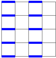
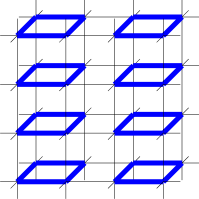
Figure 1: The studied dimerized quantum antiferromagnetic Heisenberg models: 2D ladder (left) and 3D plaquette (right) models. The bold and thin bonds shown in both sub-figures represent $J^{\prime}$ and $J$ couplings, respectively.

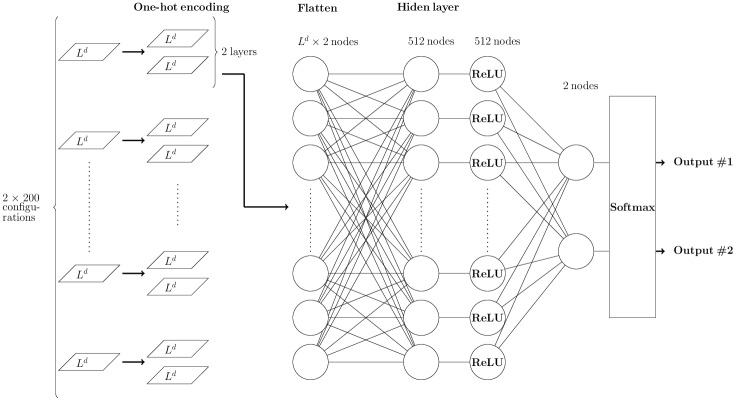
Figure 2: The NN (MLP), which consists of one input layer, one hidden layer, and one output layer, used here and in Ref. Tan20.1 . In the figure $d$ is the dimensionality of the considered system. In addition, the objects in the input layer are made up of 200 copies of only two configurations for all the studied models. Finally, there are 512 (or 1024) nodes in the hidden layer and each of these nodes is independently connected to every object in the input layer. Before each training object is connected to the nodes in the hidden layer, the steps of one-hot encoding and flatten are applied. The activation functions (ReLU and softmax) and where they are employed are demonstrated explicitly. For all the considered systems, the output layers consist of two elements.

II The microscopic models and observables

II.1 The 3D classical $O(3)$ (Heisenberg) and 2D classical XY model

The Hamiltonian $H_{O(3)}$ of the 3D classical $O(3)$ (Heisenberg) model on a cubical lattice considered in our study is given by

$$\beta H_{O(3)}=-\beta\sum_{\left<ij\right>}\vec{s}_{i}\cdot\vec{s}_{j},$$ (1)

where $\beta$ is the inverse temperature and $\left<ij\right>$ stands for the nearest neighboring sites $i$ and $j$. In addition, in Eq. (1) $\vec{s}_{i}$ is a unit vector belonging to a 3D sphere $S^{3}$ and is located at site $i$.

Starting with an extremely low temperature, as $T$ rises, the classical $O(3)$ system will undergo a phase transition from an ordered phase, where majority of the unit vectors point toward the same direction, to a disordered phase for which these mentioned vectors are oriented randomly. Relevant observables used here to signal out the phenomenon of this phase transition are the first and the second Binder ratios ($Q_{1}$ and $Q_{2}$) defined by

$$Q_{1} = \langle|m|\rangle^{2}/\langle m^{2}\rangle,$$ (2)

$$Q_{2} = \langle m^{2}\rangle^{2}/\langle m^{4}\rangle,$$ (3)

where $m=\frac{1}{L^{3}}\sum_{i}\vec{s}_{i}$ and $L$ is the linear box size of the system Bin81 .

The Hamiltonian of the 2D classical XY model on the square lattice has the same expression as $H_{O(3)}$, except that the corresponding unit vector $\vec{s}_{i}$ at site $i$ belongs to a (2D) circle instead of a 3D sphere.

II.2 The 2D and 3D dimerized quantum antiferromagnetic Heisenberg models

The 2D and 3D dimerized quantum antiferromagnetic Heisenberg model share a similar form of Hamiltonian given as

$$H=\sum_{\langle i,j\rangle}J_{ij}\vec{S}_{i}\cdot\vec{S_{j}},$$ (4)

where again $\langle i,j\rangle$ stands for the nearest neighboring sites $i$ and $j$, $J_{ij}>0$ is the associated antiferromagnetic coupling (bond) connecting $i$ and $j$, and $\vec{S}_{i}$ is the spin-1/2 operator located at $i$. The cartoon representation, in particular the spatial arrangement of the antiferromagnetic couplings, of the studied models are shown in fig. 1 (In this study, these quantum spin models will be called 2D ladder and 3D plaquette models if no confusion arises). From the figure one sees that, as the ratios $J^{\prime}/J$ (of both models) being tuned, quantum phase transitions from ordered to disordered states will take place in these models when $g\coloneqq J^{\prime}/J$ exceed certain values $g_{c}$. Relevant observables considered in our investigation for studying the quantum phase transitions are again the first and the second Binder ratios described above. For the studied spin-1/2 systems, $Q_{1}$ and $Q_{2}$ have the following definitions

$$Q_{1} = \langle|M_{s}|\rangle^{2}/\langle M_{s}^{2}\rangle,$$ (5)

$$Q_{2} = \langle M_{s}^{2}\rangle^{2}/\langle M_{s}^{4}\rangle,$$ (6)

$$M_{s} = \frac{1}{L^{d}}\sum_{i}(-1)^{i_{1}+i_{2}}S_{i}^{z},$$ (7)

here $d$ is the dimensionality of the studied models.

These mentioned $g_{c}$ of the quantum spin systems, as well as the $T_{c}$ of the 3D classical $O(3)$ and 2D classical XY models introduced previously, have been calculated with high accuracy in the literature Hol92 ; Cam02 ; Has05 ; San10 ; Tan18 .

III The constructed supervised Neural Networks

In this section, we will review the supervised NN, namely the multilayer perceptron (MLP) used in our study. The employed training sets and the associated labels for the studied models will be described as well.

III.1 The built multilayer perceptron (MLP)

The MLP used in our investigation is already detailed in Ref. Tan20.1 . Specifically, using the NN library keras kera , we construct a supervised NN which consists of only one input layer, one hidden layer of 512 (or 1024) independent nodes, and one output layer. In addition, The algorithm, optimizer, and loss function considered in our calculations are the minibatch, the adam, and the categorical cross entropy, respectively. To avoid overfitting, we also apply $L_{2}$ regularization at various stages. The activation functions employed here are ReLU and softmax. The details of the constructed MLP, including the steps of one-hot encoding and flatten (and how these two processes work) are shown in fig. 2 and are available in Ref. Tan20.1 .

Finally, for the three studied models, results calculated using 10 sets of random seeds are all taken into account when presenting the final outcomes. We would like to point out that in the testing stage, each of these 10 calculations uses the same set of configurations produced from the Monte Carlo simulations. Later we will come back to this and make a comment about it.

III.2 Training set and output labels for the 3D classical $O(3)$ and 2D classical XY models

Regarding the training set employed in the calculations, instead of using real configurations obtained from simulations or the theoretical ground states in the ordered phase of the considered system, here we use a slightly different alternative. Specifically, to train the NN on a $L$ by $L$ by $L$ cubical lattice for the 3D classical $O(3)$ model, the training set consists of only two configurations. In addition, 0 is assigned to every site of one configuration and the other configuration is made up by giving each of its sites the value of 1. As a result, the output labels are the vectors of $(1,0)$ and $(0,1)$. The same configurations and labels are employed for the 2D classical XY model as well. The motivation for considering such training sets will be explained in next subsection.

III.3 The expected output vectors for the 3D classical $O(3)$ and 2D classical XY models at various $T$

It should be pointed out that an $O(3)$ configuration is specified completely by the associated two parameters, namely $\theta$ and $\psi$ at each site of the underlying cubical lattice. At an extremely low temperature $T$, all the unit vectors of a $O(3)$ configuration point toward a particular direction. Under such a circumstance, $\psi$ mod $\pi$ is either 0 or 1 for every unit vector (of an $O(3)$ configuration). The employed training set described in the previous subsection is motivated by this observation. As a result, the magnitude $R$ of the output vector for a ground state $O(3)$ configuration is 1. When the temperature rises, one expects that $R$ diminishes with $T$ and for $T\geq T_{c}$, $R$ takes its possible minimum value $1/\sqrt{2}$. Consequently, studying the magnitude of the NN output vectors as a function of $T$ can reveal certain relevant information of $T_{c}$.

Here we would like to emphasize the fact that $\psi$ rather than $\theta$ is considered in our investigation. This is because for any two given fixed values of $\psi$, their related arc length on the 3D unit sphere are the same. For $\theta$, this is not the case. Therefore, with $\psi$ one should arrive at more accurate outcomes.

The same scenario described above for the 3D classical $O(3)$ model applies to the 2D classical XY model as well.

III.4 Training set and output labels for the 2D and 3D quantum spin models

For the 2D and 3D dimerized quantum antiferromagnetic Heisenberg models investigated here, their associated classical ground state configurations (in the order phase) are adopted as the training set. Specifically, the training set for each of these two models consists of two configurations. Moreover, the spin value of every lattice site is either 1 or -1 and they are arranged alternatively. In other words, for a site which has a spin value 1 (-1), the spin values for all of its nearest neighbor sites are -1 (1). With such set up of the training sets, the employed output vectors should be $(1,0)$ and $(0,1)$ naturally.

We would like to emphasize the fact that the training sets considered for the studied 2D and 3D quantum spin models are not even among any of the possible ground state configurations of these two systems.

III.5 The expected output vectors for the 2D and 3D dimerized quantum spin models at various $g$

Due to quantum fluctuations, it is not possible to assign any definite spin configurations for these investigated quantum spin models when $g=1$ and $g>g_{c}$. Therefore, how the corresponding output vectors behave with respect to the dimerized strength $g$ will be treated classically here. Consequently, $R$ should be 1 and $1/\sqrt{2}$ for $g=1$ and $g\geq g_{c}$, respectively. As we will demonstrate shortly, the $R$ (magnitude) of the outputs associated with the NN studies of these quantum spin systems follow these rules (i.e., the values of $R$ are 1 and $1/\sqrt{2}$ for $g=1$ and $g>g_{c}$, respectively) in a satisfactory manner, hence lead to fairly good estimations of the critical points.

IV The numerical results

The configurations associated with the considered systems, namely the 3D (classical) $O(3)$, the 2D classical XY, the 3D plaquette, as well as the 2D ladder models are generated by the Wolff and the stochastic series expansion (SSE) algorithms Wol89 ; San99 ; San10 . In addition, for each of the studied model, the corresponding configurations are recorded once in (at least) every two thousand Monte Carlo sweeps after the thermalization, and at least one thousand configurations are produced. These spin compositions are then used for the calculations of NN. A semi-experimental finite-size scaling, which is adopted to estimate the critical points, will be introduced as well in this section.

IV.1 Results of 3D classical $O(3)$ model

In fig. 3, the observable first Binder ratio $Q_{1}$ are considered as functions of $\beta$ for $L=8,12,16$. As can be seen from the figure, the curves corresponding to various $L$ intersect at a value of $\beta$ close to the predicted critical point $\beta_{c}=0.6929$ Hol92 ; Cam02 .

For a $O(3)$ configuration obtained from the simulation, all the $S^{3}$ vectors associated with it are converted to $\psi$ mod $\pi$ and the resulting configuration is then fed into the trained NN.

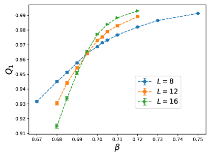
Figure 3: $Q_{1}$ as functions of $\beta$ for the 3D classical $O(3)$ model.

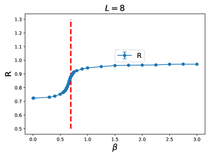
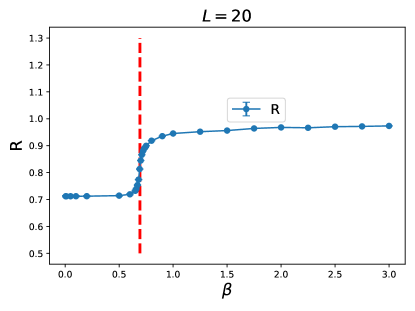
Figure 4: $R$ as functions of $\beta$ for the 3D classical $O(3)$ model. The top and bottom panels are for $L=8$ and $L=20$, respectively.

$R$ as functions of $\beta$ for $L=8$ and $L=20$ are shown in fig. 4. While it is clear that both panels of fig. 4 imply $R$ change rapidly close to $\beta_{c}=0.6929$, $\beta_{c}$ cannot be calculated unambiguously when only the information of $R$ is available.

If one assumes that $R$ diminishes linearly with $\beta$ in the critical region, then $\beta_{c}$ can be approximately estimated by the intersection of the curves of $R$ and $1/\sqrt{2}+1-R$. Such an idea has been used in Ref. Tan20.1 to calculate the $T_{c}$ of the 3D 5-state ferromagnetic Potts model as well as the $g_{c}$ of the 3D plaquette model (the latter will be studied in more detail here). Here we adopt a more appropriate approach for the determination of the considered critical points by taking into account the deviation between the theoretical and the calculated $R$.

Ideally, at extremely low temperature region, the obtained $R$ should be 1. To fulfill this criterion, an overall shift $\Delta$, which is the difference between $1$ and the $R$ from the simulation with the largest $\beta$, is conducted delta . Figures 5 and 6 demonstrate the associated curves made up of considering the data of $R+\Delta$ and $1/\sqrt{2}+1-R-\Delta$ as functions of $\beta$ for $L=4,8,12,20,24$. As can be seen from the figures, the intersections of these two curves for all the $L$ (except the one of $L=4$) are in good agreement with the theoretical prediction $\beta_{c}\sim 0.693$ (which are the vertical dashed lines in these figures). While for large $L$, the estimated values of $\beta$ at which the mentioned two curves intersect are slightly away from $\beta_{c}=0.6929$, the results shown in figs. 5 and 6 indicate that the idea of estimating $\beta_{c}$ by considering the intersection of the curves associated with $R+\Delta$ and $1/\sqrt{2}+1-R-\Delta$ is an effective approach. In particular, considering the simplicity of both the training procedure and the semi-experimental method of calculating $\beta_{c}$ (for any finite $L$) employed in this study, the achievement reaches here for the determination of the $T_{c}$ of the complicated 3D classical $O(3)$ model is remarkable.

The success of calculating the $T_{c}$ of 3D classical $O(3)$ model through the idea of only considering $\psi$ mod $\pi$ indicates that partial information of the model is sufficient to estimate its associated critical point accurately.

To calculate the critical points of the studied models with high precision using the intersections described above, one may apply certain forms of finite-size scaling to those crossing points. Based on the outcomes demonstrated in figs. 5 and 6, it is clear that the $R$ associated with the 3D classical $O(3)$ model receives mild finite-size effect. Apart from this, accurate determination of the crossing places in the relevant parameter space, particularly high precision estimated uncertainties for these crossing points, is needed in order to carry out the fits. Hence we postpone such an analysis to a latter subsection where 2D 3-state ferromagnetic Potts model and 2D classical XY models on the square lattices are discussed.

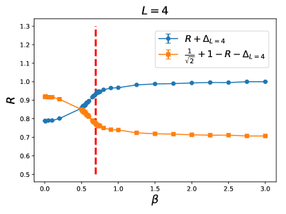
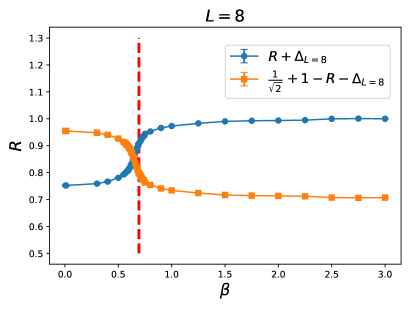
Figure 5: $R+\Delta$ and $1/\sqrt{2}-\Delta+1-R$ as functions of $\beta$ for the 3D classical $O(3)$ model. The top and bottom panels are for $L=4$ and $L=8$, respectively.

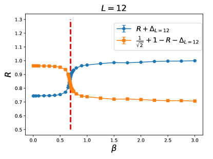
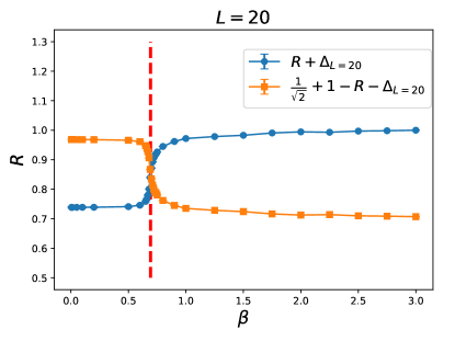
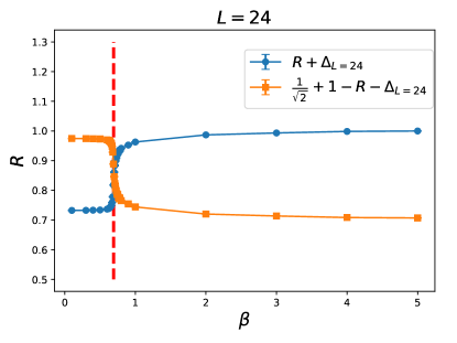
Figure 6: $R+\Delta$ and $1/\sqrt{2}-\Delta+1-R$ as functions of $\beta$ for the 3D classical $O(3)$ model. The top, middle, and bottom panels are for $L=12$, $L=20$, and $L=24$, respectively.

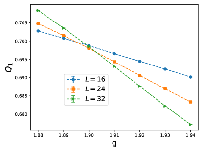
Figure 7: $Q_{1}$ (of $L=16,24,32$) as functions of $g$ for the 2D dimerized quantum ladder model.

IV.2 Results of 2D quantum spin system

The first Binder ratio $Q_{1}$ close to $g_{c}$ for the studied 2D dimerized spin-1/2 antiferromagnet (2D ladder model) are shown in fig. 7. Similar to the case of 3D classical $O(3)$ model, various curves of large $L$ tend to intersect at a value of $g$ around 1.9. The estimated intersection $g\sim$ 1.9 matches nicely with the known result $g_{c}=1.90948(5)$ in the literature San10 . Of course, a better determination of $g_{c}$ requires the performance of a dedicated finite-size scaling analysis.

For the 2D ladder model, the associated $R$ as functions of $g$ for $L=24,48$ are shown in fig. 8. Moreover, by using the idea of estimating $\beta_{c}$ for the 3D classical $O(3)$ model, the curves resulting from treating $R+\Delta$ and $1/\sqrt{2}+1-R-\Delta$ as functions of $g$ are demonstrated in figs. 9 ($L=24,32$) and 10 ($L=48,64$). The vertical dashed lines in these figures are the theoretical $g_{c}$. Here $\Delta$ is the difference between the theoretical and the calculated values of $R$ at $g=1$. As can be seen from the figures, when box size $L$ increases, the $g$ at which the mentioned two curves intersects is approaching the theoretical $g_{c}$. Hence the outcomes demonstrated in the figures support the fact that our method of determining the critical points is also valid for the investigated quantum (spin) system.

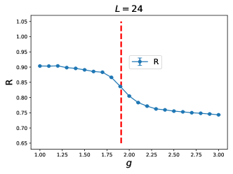
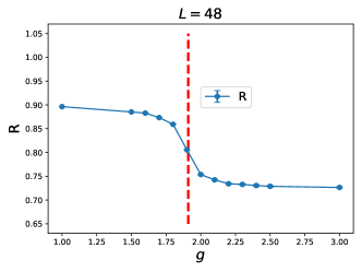
Figure 8: $R$ as functions of $g$ for the 2D dimerized quantum ladder model. The top and bottom panels are for $L=24$ and $L=48$, respectively.

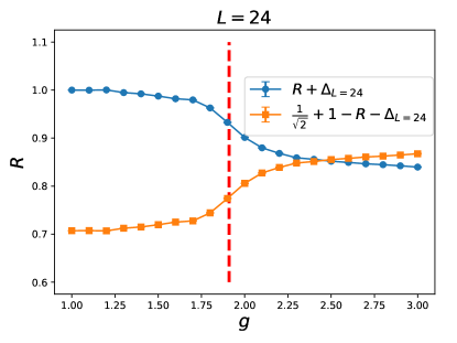
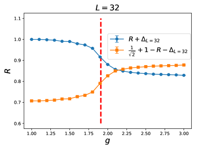
Figure 9: $R+\Delta$ and $1/\sqrt{2}-\Delta+1-R$ as functions of $g$ for the 2D dimerized quantum ladder model. The top and bottom panels are for $L=24$ and $L=32$, respectively.

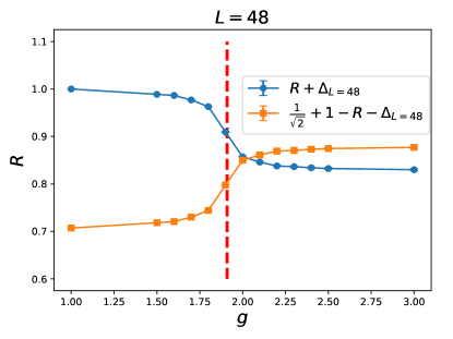
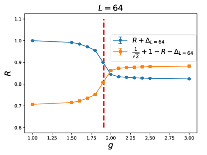
Figure 10: $R+\Delta$ and $1/\sqrt{2}-\Delta+1-R$ as functions of $g$ for the 2D dimerized quantum ladder model. The top and bottom panels are for $L=48$ and $L=64$, respectively.

IV.3 Results of 3D quantum spin system

The $g_{c}$ of the 3D plaquette model studied in Ref. Tan18 can be determined by considering the Néel temperatures $T_{N}$ of various $g$ close to $g_{c}$. Specifically, if the logarithmic correction is not taken into account, then close to $g_{c}$, $T_{N}$ can be described by $T_{N}\sim A|g-g_{c}|^{c}+B|g-g_{c}|^{2c}$, here $A$, $B$, and $c$ are some constants. As a result, $g_{c}$ can be calculated by fitting the data of $T_{N}$ of various $g$ to this form. The $g_{c}$ estimated by this approach lies between 4.35 and 4.375, see fig. 11. This obtained $g_{c}$ will be used to examine the effectiveness of the NN method of calculating the $g_{c}$ of the 3D plaquette model.

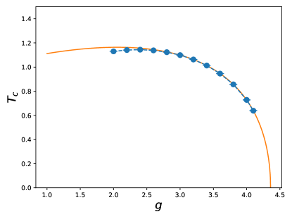
Figure 11: $T_{N}$ as a function of $g$ for the 3D dimerized quantum plaquette model. The solid line shown in the figure is obtained by using the results from a fit.

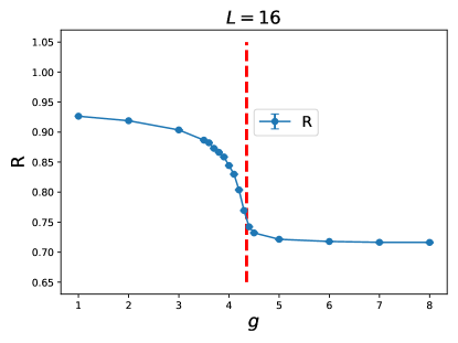
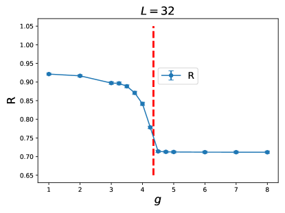
Figure 12: $R$ as functions of $g$ for the 3D dimerized quantum plaqutte model. The top and bottom panels are for $L=16$ and $L=32$, respectively.

$R$ as functions of $g$ for $L=16$ and 32 for the 3D plaquette model are shown in fig. 12. In addition, the curves resulting from considering $R+\Delta$ and $1/\sqrt{2}+1-R-\Delta$ as functions of $g$ are demonstrated in fig. 13 ($L=16,32$). The vertical dashed lines in these figures are 4.35 which is the estimated lower bound for $g_{c}$ discussed in the previous paragraph. Here $\Delta$ is again the difference between the theoretical and the calculated values of $R$ at $g=1$.

Remarkably, just like what we have found for the 2D quantum ladder model, the results shown in the figure clearly reveal the message that our NN method is valid for 3D quantum spin model as well.

It is interesting to notice that the crossing points in both panels of fig. 13 are slightly below the critical point calculated from $T_{N}$. We attribute this to the facts that the systematic influence of some tunable parameters of NN as well as certain corrections to the employed finite-size scaling method are not taken into account here.

Nevertheless, based on the outcomes associated with both the investigated 2D and 3D dimerized quantum antiferromagnetic Heisenberg models, it is beyond doubt that the NN approach employed here can be used to estimate the critical points of quantum phase transitions efficiently.

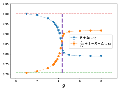
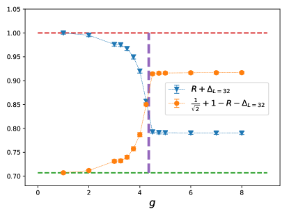
Figure 13: $R+\Delta$ and $1/\sqrt{2}-\Delta+1-R$ as functions of $g$ for the 3D dimerized quantum plaquette model. The top and bottom panels are for $L=16$ and $L=32$, respectively.

IV.4 Verification of the semi-experimental finite-size scaling formulas: 2D three-state ferromagnetic Potts model and 2D classical XY model on the square lattices

IV.4.1 2D three-state ferromagnetic Potts model

In previous subsections, it is shown that the critical point can be obtained by considering the intersection of two curves made up of quantities associated with $R$. To obtain a high precision estimation for the critical point using the crossing points, one can apply certain expression of finite-size scaling to fit the data (of the crossing points). Here we use the data of the 2D 3-state ferromagnetic Potts model on the square lattice available in Ref. Li18 to carry out such an investigation. For each $L$, the data are obtained using a single set of relevant NN parameters. As a result, the quoted errors are associated with the Potts configurations themselves.

Figure 14 shows that data of $R+\Delta$ and $1/\sqrt{3}+1-R-\Delta$ as functions of $T$ for various $L$ for the 2D 3-state ferromagnetic Potts model on the square lattice Li18 . A fit of the form $a+b/L^{c}$, where $a$, $b$, and $c$ are some to be determined constants ($a$ is exactly the desired $T_{c}$), is used to fit the data of the crossing points obtained from $L=10,20,40,80,120,240$ (The data of $L=120$ and 240 are not presented in fig. 14). When carrying out the fits, Gaussian noises are considered in order to estimate the corresponding errors of the constants $a$, $b$, and $c$.

The fits lead to $a=0.995(3)$ which agrees quantitatively with the theoretical prediction $T_{c}\sim 0.99497$, see fig. 15. This in turn confirms the validity of calculating the critical points using the NN approach presented in this study.

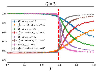
Figure 14: $R+\Delta$ and $1/\sqrt{3}+1-R-\Delta$ as functions of $T$ for various $L$ for the 2D 3-state ferromagnetic Potts model on the square lattice.

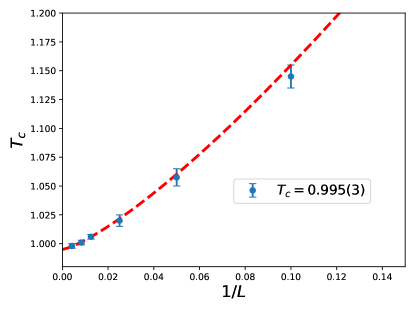
Figure 15: Fit of the crossing points (of various finite $L$) to the ansatz $a+b/L^{c}$. The data are associated with the 3-state ferromagnetic Potts model on the square lattice Li18 and the dashed line in the figure is obtained by using the results of the fits.

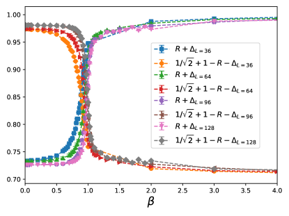
Figure 16: $R+\Delta$ and $1/\sqrt{2}+1-R-\Delta$ as functions of $\beta$ for various $L$ for the 2D classical XY model on the square lattice.

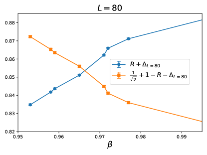
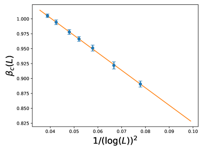
Figure 17: (Top) Estimation of the crossing point for $L=80$. (Bottom) Fit of $\beta_{c}(L)$ to the ansatz $a_{1}+b_{1}/\left(\log(L)\right)^{2}$. The solid line is obtained using the results from the fit.

IV.4.2 2D classical XY model

The $R+\Delta$ and $1/\sqrt{2}+1-R-\Delta$ as functions of $\beta$ for several $L$ of the 2D classical XY model are demonstrated in fig. 16. Similar to the analysis done for the 2D 3-state ferromagnetic Potts model, we would like to calculate the crossing points for various $L$ and use some kind of finite-size scaling to fit the obtained data so that one can determine the associated $\beta_{c}$ (or $T_{c}$). After obtaining coarse estimations of the crossing points for various $L$ from fig. 16, more simulations are carried out in order to reach a better precision for these crossing points. These refined $\beta_{c}(L)$ are then fitted to the same formula (i.e. $a+b/L^{c}$) as that used for the 3-state Potts model. We find that the obtained results are not satisfactory. This can be expected since the topological characteristics of the Kosterlitz-Thouless transition should reflect on $R$.

Motivated by the finite-size scaling formulas used in Refs. Bea18 ; Has05 ; Hsi13 for the 2D classical XY model, we use a ansatz of the form $a_{1}+b_{1}/(\log(L))^{2}$ (here $a_{1}$ is the $\beta_{c}$) to fit the newly obtained data of crossing points. The outcome is good and we find the $\beta_{c}$ is given by $\beta_{c}=1.119(7)$ (see both panels of fig. 17) which match very well with the known result $\beta_{c}\sim 1.1199$ in the literature. It is intriguing that the simple NN procedure used here works for the phase transition(s) associated with topology as well.

Before ending this subsection, we would like to point out that in principle the supervised NN method is a optimization procedure. As a result, to obtain a more accurate estimation of the critical point in a (supervised) NN investigation, the systematic impact associated with the tunable parameters of a built NN, such as the number of epoch, batchsize, nodes in the hidden layers and so on, should be examined.

V Discussions and Conclusions

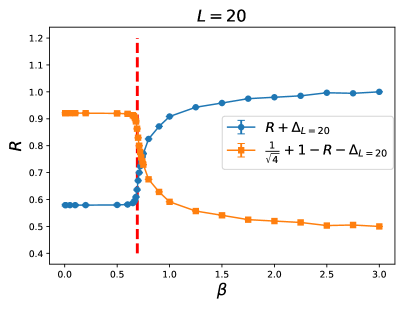
Figure 18: $R+\Delta$ and $1/\sqrt{4}-\Delta+1-R$ as functions of $\beta$ for the 3D classical $O(3)$ model. The results are obtained from the calculations which use 4 configurations as the training set.

In this study we investigate the phase transitions of 3D classical $O(3)$ model and 2D classical XY model, as well as the quantum phase transitions of both 2- and 3-D dimerized spin-1/2 antiferromagnetic Heisenberg models using the simplest deep learning NN, namely a MLP that is made up of only one input layer, one hidden layer, as well as one output layer.

In our investigation, the training set for each of the studied models consists of only two objects. In particular, none of the used training objects belongs to the theoretical or the real configurations of the considered physical systems.

Remarkably, with such an unconventional approach of carrying out the training processes in conjunction with semi-experimental finite-size scaling formulas, the resulting outcomes from the built MLP lead to very good estimations of the targeted critical points. The results reached here as well as that shown in Refs. Li18 ; Tan20.1 provide convincing evidence that the performance of certain unconventional strategies, such as employing the theoretical ground state configurations as the training sets, are impressive. Particularly, the simplicity of these approaches make them cost-effective in computation. It is amazing that the simple procedures used in Refs. Li18 ; Tan20.1 and here are not only valid for phase transitions associated with SSB, but also work for those related to topology.

We would like to point out that for the 3D classical $O(3)$ model, the training set used here consists of two configurations (their elements are either all 1 or all 0). In principle, one can consider training set made up of three, four, or even five configurations following the same idea as that of two objects training set. To examine whether using the training sets, which constitute more than two objects, one can arrive at the same level of success as that shown in the previous section, we have performed three more NN calculations using $n=3$, $n=4$, and $n=5$ training sets. Here $n$ denotes the number of objects containing in the training set. Interestingly, the precision of the estimated $T_{c}$ of the 3D classical $O(3)$ model obtained from these additional calculations is becoming slightly less satisfactory with $n$, see fig. 18 for a outcome related to $n=4$ and $L=20$. Intuitively, this can be understood as follows. Let us assume that initially all the unit vectors belong to a category of the classification scheme implemented in the training stage. Then any local fluctuation will have greater impact on the resulting NN outputs if the training set contains more types of objects. Despite this, it is beyond doubt that the outcomes associated with training sets consisting of only 2 configurations, including those from all the three studied models, strongly suggest the effectiveness of the approach presented in this study.

The NN results related to all the models considered here are obtained using 10 sets of random seeds with other parameters of NN being fixed in the calculations. For several $L$ of the studied 3D $O(3)$ and 2D ladder models, we have performed analysis using only one of the 10 trained NNs. Some of the resulting outcomes are shown in figs. 19, 20 (The errors of the data shown in these new figures are associated with the configurations determined from QMC simulations). These new figures match nicely with that determined with 10 sets of random seeds. Apart from this, we have also carried out several calculations using various batchsize, epoch, and nodes in the hidden layer. These new calculations lead to very good agreement with that shown explicitly in this study as well, see fig. 21 for one result from these new calculations. The additional investigations introduced in this paragraph imply that the tunable parameters of NN have very mild effects on the resulting outcomes of $R$ for the considered models. Hence the obtained conclusion here should be reliable. Of course, as already being pointed out before, considering other systematic impacts are required if a highly accurate estimation of the targeted critical point is desirable.

Figure 19: $R+\Delta$ and $1/\sqrt{2}-\Delta+1-R$ as functions of $\beta$ for the 3D classical $O(3)$ model. The data are obtained using only one set of random seeds. The top and bottom panels are for $L=4$ and $L=24$, respectively.

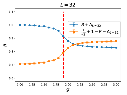
Figure 20: $R+\Delta$ and $1/\sqrt{2}-\Delta+1-R$ as a function of $g$ for the 2D ladder model. The data are obtained using only one set of random seeds.

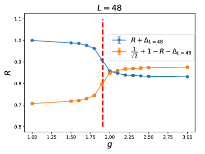
Figure 21: $R+\Delta$ and $1/\sqrt{2}-\Delta+1-R$ as a function of $g$ for the 2D ladder model. The data are obtained using different NN parameters from that shown in the previous subsection.

Although in this study we have focused on studying the phase transitions of several models, it is probable that simple NN approaches, similar to the one(s) considered here, are available for investigating other physical properties of many-body systems. Finally, we would like to emphasize the motivations for the series of our studies of applying the NN techniques to investigate the phase transitions of several physical systems, as shown in Refs. Li18 ; Tan20.1 and here. Conventionally, the application of a supervised NN to explore the critical phenomenon of a specific system has a caveat, namely the knowledge of the critical point is required in advance before one can employ the methods of NN for the investigation. Hence for systems with unknown critical points, it may not be easy to apply such standard NN procedures to the studies in a straightforward manner. The approaches considered in Refs. Li18 ; Tan20.1 and here definitely can take care of this issue, hence promote the use of NN methods in various fields of many-body systems. In particular, these unconventional methods are adequate for carrying out any NN investigations of examining whether certain proposed theories are relevant for a real and unexplored physical system.

References

- (1) Matthias Rupp, Alexandre Tkatchenko, Klaus-Robert Müller, and O. Anatole von Lilienfeld, Phys. Rev. Lett. 108 058301 (2012).
- (2) John C. Snyder, Matthias Rupp, Katja Hansen, Klaus-Robert Müller, and Kieron Burke, Phys. Rev. Lett. 108 253002 (2012).
- (3) Grégoire Montavon, Matthias Rupp, Vivekanand Gobre, Alvaro Vazquez-Mayagoitia, Katja Hansen Alexandre Tkatchenko, Klaus-Robert Muller, and O. Anatole von Lilienfeld, New Journal of Physics 15 (2013) 095003.
- (4) Pilania, G., Wang, C., Jiang, X. et al., Sci Rep 3, 2810 (2013).
- (5) B. Meredig, A. Agrawal, S. Kirklin, J. E. Saal, J. W. Doak, A. Thompson, K. Zhang, A. Choudhary, and C. Wolverton, Phys. Rev. B 89, 094104 (2014).
- (6) K. T. Schütt, H. Glawe, F. Brockherde, A. Sanna, K. R. Müller, and E. K. U. Gross, Phys. Rev. B 89, 205118 (2014).
- (7) Zhenwei Li, James R. Kermode, and Alessandro De Vita, Phys. Rev. Lett. 114, 096405 (2015)
- (8) P. Baldi, P. Sadowski and D. Whiteson, Phys. Rev. Lett. 114, 111801 (2015).
- (9) V. Mnih, K. Kavukcuoglu, D. Silver, A. A. Rusu, J. Veness, M. G. Bellemare, A. Graves, M. Riedmiller, A. K. Fidjeland, G. Ostrovski, S. Petersen, C. Beattie, A. Sadik, I. Antonoglou, H. King, D. Kumaran, D. Wierstra, S. Legg and D. Hassabis, Nature 518, no.7540, 529-533 (2015).
- (10) Tobias Lang, Florian Flachsenberg, Ulrike von Luxburg, and Matthias Rarey, J. Chem. Inf. Model. 2016, 56, 1, 12–20.
- (11) Joohwi Lee, Atsuto Seko, Kazuki Shitara, Keita Nakayama, and Isao Tanaka, Phys. Rev. B 93, 115104 (2016).
- (12) J. Searcy, L. Huang, M. A. Pleier and J. Zhu, Phys. Rev. D 93, no.9, 094033 (2016).
- (13) T. Castro, M. Quartin and S. Benitez-Herrera, Phys. Dark Univ. 13 (2016), 66-76.
- (14) P. Baldi, K. Cranmer, T. Faucett, P. Sadowski and D. Whiteson, Eur. Phys. J. C 76, no.5, 235 (2016).
- (15) P. Baldi, K. Bauer, C. Eng, P. Sadowski and D. Whiteson, Phys. Rev. D 93, 094034 (2016).
- (16) Giacomo Torlai and Roger G. Melko, Phys. Rev. B 94, 165134 (2016).
- (17) Lei Wang, Phys. Rev. B 94, 195105 (2016)
- (18) M. Attarian Shandiz and R. Gauvin Computational Materials Science 117 (2016) 270-278.
- (19) Tomoki Ohtsuki and Tomi Ohtsuki, J. Phys. Soc. Jpn. 85, 123706 (2016).
- (20) B. Hoyle, Astron. Comput. 16, 34-40 (2016).
- (21) Juan Carrasquilla, Roger G. Melko, Nature Physics 13, 431–434 (2017).
- (22) Giuseppe Carleo, Matthias Troyer, Science 355, 602 (2017)
- (23) Zhenqin Wu, Bharath Ramsundar, Evan N. Feinberg, Joseph Gomes, Caleb Geniesse, Aneesh S. Pappu, Karl Leswing and Vijay Pande, Chem. Sci., 2018, 9, 513.
- (24) Peter Broecker, Juan Carrasquilla, Roger G. Melko, and Simon Trebst, Scientific Reports 7, 8823 (2017).
- (25) Kelvin Ch’ng, Juan Carrasquilla, Roger G. Melko, and Ehsan Khatami, Phys. Rev. X 7, 031038 (2017).
- (26) J. Barnard, E. N. Dawe, M. J. Dolan and N. Rajcic, Phys. Rev. D 95, 014018 (2017).
- (27) Akinori Tanaka, Akio Tomiya, J. Phys. Soc. Jpn. 86, 063001 (2017).
- (28) Evert P.L. van Nieuwenburg, Ye-Hua Liu, Sebastian D. Huber, Nature Physics 13, 435–439 (2017)
- (29) A. Mott, J. Job, J. R. Vlimant, D. Lidar and M. Spiropulu, Nature 550, no.7676, 375-379 (2017).
- (30) Junwei Liu, Huitao Shen, Yang Qi, Zi Yang Meng, Liang Fu, Phys. Rev. B 95, 241104(R) (2017).
- (31) Tomoyuki Tamura et al (2017) Modelling Simul. Mater. Sci. Eng. 25 075003.
- (32) J. Tubiana and R. Monasson, Phys. Rev. Lett. 118, 138301 (2017).
- (33) Xiao Yan Xu, Yang Qi, Junwei Liu, Liang Fu, Zi Yang Meng, Phys. Rev. B 96, 041119(R) (2017).
- (34) Li Huang and Lei Wang, Phys. Rev. B 95, 035105 (2017).
- (35) M. Zevin, S. Coughlin, S. Bahaadini, E. Besler, N. Rohani, S. Allen, M. Cabero, K. Crowston, A. Katsaggelos, S. Larson, T. K. Lee, C. Lintott, T. Littenberg, A. Lundgren, C. Østerlund, J. Smith, L. Trouille and V. Kalogera, Class. Quant. Grav. 34, no.6, 064003 (2017).
- (36) Junwei Liu, Yang Qi, Zi Yang Meng, Liang Fu, Phys. Rev. B 95, 041101 (2017).
- (37) Yue Liu, Tianlu Zhao. Wangwei Ju, Siqi Shi, J. Materiomics 3 (2017) 159-177.
- (38) Qianshi Wei, Roger G. Melko, Jeff Z. Y. Chen, Phys. Rev. E 95, 032504 (2017).
- (39) Yuki Nagai, Huitao Shen, Yang Qi, Junwei Liu, and Liang Fu Phys. Rev. B 96 161102 (2017).
- (40) Kolb, B., Lentz, L. C. and Kolpak, A. M., Sci Rep 7, 1192 (2017).
- (41) Dong-Ling Deng, Xiaopeng Li, and S. Das Sarma, Phys. Rev. B 96 195145 (2017).
- (42) Pedro Ponte and Roger G. Melko, Phys. Rev. B 96, 205146 (2017).
- (43) G. Kasieczka, T. Plehn, M. Russell and T. Schell, JHEP 05, 006 (2017).
- (44) Yi Zhang, Roger G. Melko, and Eun-Ah Kim Phys. Rev. B 96, 245119 (2017).
- (45) Yi Zhang and Eun-Ah Kim, Phys. Rev. Lett. 118, 216401 (2017)
- (46) Wenjian Hu, Rajiv R. P. Singh, and Richard T. Scalettar, Phys. Rev. E 95, 062122 (2017).
- (47) C.-D. Li, D.-R. Tan, and F.-J. Jiang, Annals of Physics, 391 (2018) 312-331.
- (48) Kelvin Ch’ng, Nick Vazquez, and Ehsan Khatami, Phys. Rev. E 97, 013306 (2018).
- (49) Lu, S., Zhou, Q., Ouyang, Y. et al., Nat Commun 9, 3405 (2018).
- (50) D. George and E. A. Huerta, Phys. Rev. D 97, 044039 (2018).
- (51) Matthew J. S. Beach, Anna Golubeva, and Roger G. Melko, Phys. Rev. B 97, 045207 (2018).
- (52) L. G. Pang, K. Zhou, N. Su, H. Petersen, H. Stöcker and X. N. Wang, Nature Commun. 9, no.1, 210 (2018).
- (53) Phiala E. Shanahan, Daniel Trewartha, and William Detmold, Phys. Rev. D 97, 094506 (2018).
- (54) Nongnuch Artrith, Alexander Urban, and Gerbrand Ceder, J. Chem. Phys. 148, 241711 (2018).
- (55) Keith T. Butler, Daniel W. Davies, Hugh Cartwright, Olexandr Isayev, and Aron Walsh, Nature 559, 547–555 (2018).
- (56) Albert P. Bartoḱ, James Kermode, Noam Bernstein, and Gab́or Csańyi, Phys. Rev. X 8, 041048 (2018).
- (57) Pengfei Zhang, Huitao Shen, and Hui Zhai, Phys. Rev. Lett. 120, 066401 (2018).
- (58) Jake Graser, Steven K. Kauwe, and Taylor D. Sparks Chem. Mater. 2018, 30, 11, 3601–3612.
- (59) A. Butter, G. Kasieczka, T. Plehn and M. Russell, SciPost Phys. 5, no.3, 028 (2018).
- (60) Jun Gao et al. Phys. Rev. Lett. 120, 240501 (2018).
- (61) Wanzhou Zhang, Jiayu Liu, and Tzu-Chieh Wei, Phys. Rev. E 99, 032142 (2019).
- (62) Jonas Greitemann, Ke Liu, and Lode Pollet, Phys. Rev. B 99, 060404 (2019).
- (63) J. Ren, L. Wu, J. M. Yang and J. Zhao, Nucl. Phys. B 943, 114613 (2019).
- (64) Xiao-Yu Dong, Frank Pollmann, and Xue-Feng Zhang, Phys. Rev. B 99, 121104 (2019).
- (65) M. Cavaglia, K. Staats and T. Gill, Commun. Comput. Phys. 25, no.4, 963-987 (2019).
- (66) Daniel W. Davies, Keith T. Butler, and Aron Walsh, Chem. Mater. 2019, 31, 18, 7221–7230.
- (67) G. P. Conangla, F. Ricci, M. T. Cuairan, A. W. Schell, N. Meyer and R. Quidant, Phys. Rev. Lett. 122, 223602 (2019)
- (68) Boram Yoon, Tanmoy Bhattacharya, and Rajan Gupta, Phys. Rev. D 100, 014504 (2019).
- (69) J. Fluri, T. Kacprzak, A. Lucchi, A. Refregier, A. Amara, T. Hofmann and A. Schneider, Phys. Rev. D 100, 063514 (2019).
- (70) Askery Canabarro, Felipe Fernandes Fanchini, André Luiz Malvezzi, Rodrigo Pereira, and Rafael Chaves, Phys. Rev. B 100, 045129 (2019).
- (71) Limeng Li, Yang You, Shunbo Hu, Yada Shi, Guodong Zhao, Chen Chen, Yin Wang, Alessandro Stroppa and Wei Ren, Appl. Phys. Lett. 114, 083102 (2019).
- (72) Henry Chan, Badri Narayanan, Mathew J. Cherukara, Fatih G. Sen, Kiran Sasikumar, Stephen K. Gray, Maria K. Y. Chan, and Subramanian K. R. S. Sankaranarayanan, J. Phys. Chem. C 2019, 123, 12, 6941–6957.
- (73) Wenqian Lian et al. Phys. Rev. Lett. 122, 210503 (2019).
- (74) Linyang Zhu, Weiwei Zhang, Jiaqing Kou, and Yilang Liu, Physics of Fluids 31, 015105 (2019).
- (75) Pankaj Mehta, Marin Bukov, Ching-Hao Wang, Alexandre G.R. Day, Clint Richardson, Charles K. Fisher, and David J. Schwab, Phys. Rep. 810, (2019) 1-124.
- (76) Schutt, K.T., Gastegger, M., Tkatchenko, A. et al., Nat Commun 10, 5024 (2019).
- (77) Joaquin F. Rodriguez-Nieva and Mathias S. Scheurer, Nat. Phys. 15, 790–795 (2019).
- (78) Giuseppe Carleo, Ignacio Cirac, Kyle Cranmer, Laurent Daudet, Maria Schuld, Naftali Tishby, Leslie Vogt-Maranto, and Lenka Zdeborová, Rev. Mod. Phys. 91, 045002 (2019).
- (79) T. Ohtsuki et al. J. Phys. Soc. Jpn. 89, 022001 (2020)
- (80) Wataru Hashimoto, Yuta Tsuji, and Kazunari Yoshizawa J. Phys. Chem. C 2020, 124, 18, 9958–9970.
- (81) Ryosuke Jinnouchi, Ferenc Karsai, and Georg Kresse Phys. Rev. B 101, 060201(R) (2020).
- (82) A. J. Larkoski, I. Moult and B. Nachman, Phys. Rept. 841, 1-63 (2020).
- (83) X. Han and S. A. Hartnoll, Phys. Rev. X 10, 011069 (2020).
- (84) D.-R. Tan et al. 2020 New J. Phys. 22 063016
- (85) Japneet Singh, Vipul Arora, Vinay Gupta, and Mathias S. Scheurer, arXiv:2006.11868.
- (86) K. Binder, Z. Phys. B bf 43, 119 (1981).
- (87) Christian Holm and Wolfhard Janke, Phys. Lett. A173 (1993) 8.
- (88) Massimo Campostrini, Martin Hasenbusch, Andrea Pelissetto, Paolo Rossi, and Ettore Vicari, Phys. Rev. B 65, 144520 (2002).
- (89) Martin Hasenbusch, J. Phys. A 38 (2005) 5869-5884.
- (90) A. W. Sandvik, AIP Conf. Proc. 2397, 135 (AIP, New York, 2010).
- (91) D.-R. Tan and F.-J. Jiang, Phys. Rev. B 97, 094405 (2018).
- (92) U. Wolff, Phys. Rev. Lett. 62, 361 (1989).
- (93) A. W. Sandvik, Phys. Rev. B 66, R14157 (1999).
- (94) https://keras.io
- (95) Based on the employed training sets, the correction should be calculated at the obtained with the largest for the 3D classical and 2D classical XY models. Similarly, the associated with the studied quantum spin models are determined at the corresponding to .
- (96) Yun-Da Hsieh, Ying-Jer Kao, A. W. Sandvik, J. Stat. Mech. (2013) P09001.