The SHIR Model: Realistic Fits to COVID-19 Case Numbers

Abstract

We consider a global (location independent) model of pandemic growth which generalizes the SIR model to accommodate important features of the COVID-19 pandemic, notably the implementation of pandemic reduction measures. This “SHIR” model is applied to COVID-19 data, and shows promise as a simple, tractable formalism with few parameters that can be used to model pandemic case numbers. As an example we show that the average time dependence of new COVID-19 cases per day from 15 Central and Western European countries is in good agreement with the analytic, parameter-free prediction of the model.

I Epidemic Models

I.1 SIR Models

In the models typically employed in epidemiology to follow the evolution of a pandemic Roc2014 , one begins by partitioning a total population of N individuals into a complete set of disjoint subsets, according to their medical histories. The simplest models of this type have only a few categories, such as 1) the susceptible but as yet uninfected population S, 2) the infected but not recovered population I, who can infect S, and 3) the recovered population R, who can no longer infect S, and can themselves no longer be infected. First-order ordinary differential equations (ODEs) in time are assumed to describe the coupling between these groups. Once the appropriate initial conditions are specified, these ODEs can be integrated, which gives predictions for the subsequent evolution of the group populations.

In this example, given constant rates $\{r_{ij}\}$ for the two assumed transitions, $\rm S\to\rm I$ and $\rm I\to\rm R$, the resulting ODEs for this simple “SIR” model are

$$d{\rm S}/dt =-r_{\rm S\to\rm I}\rm S$$ (1)

$$d{\rm I}/dt =+r_{\rm S\to\rm I}\rm S-r_{\rm I\to\rm R}\rm I$$ (3)

$$d{\rm R}/dt =+r_{\rm I\to\rm R}\rm I$$ (5)

We will refer to these two rate coefficients as $r_{\rm S\to\rm I}=r_{\rm I}$ and $r_{\rm I\to\rm R}=r_{\rm R}$. On adding these equations we find that

$$d{\rm S}/dt+d{\rm I}/dt+d{\rm R}/dt=d{\rm N}/dt=0\ ,$$ (6)

so the total number of individuals is a constant, $\rm N_{0}$.

Since these equations are linear and homogeneous, it is convenient to divide by $\rm N_{0}$ and solve for the fraction of individuals in each category, such as $f_{\rm S}={\rm S}/\rm N_{0}$. R or $f_{\rm R}$ can be inferred from the other two populations, using $\rm R=\rm N_{0}-\rm S-\rm I$, or equivalently $f_{\rm R}=1-f_{\rm S}-f_{\rm I}$, so we need only solve the set (9),

$$df_{\rm S}/dt =-r_{\rm I}f_{\rm S}\ ,$$ (7)

$$df_{\rm I}/dt =+r_{\rm I}f_{\rm S}-r_{\rm R}f_{\rm I}\ .$$ (9)

We will assume that the entire population is initially in category S (susceptible but not infected or recovered), so that $f_{\rm S}(t=0)=1$ and $f_{\rm I}(t=0)=0$. Given these initial conditions we can solve the equations (9), which also imply $f_{\rm R}$ through $f_{\rm R}=1-f_{\rm S}-f_{\rm I}$, with the results

$$f_{\rm S}(t) =e^{-r_{\rm I}t}$$ (10)

$$f_{\rm I}(t) =\frac{r_{\rm I}}{r_{\rm R}-r_{\rm I}}\Big{(}e^{-r_{\rm I}t}-e^{-r_{\rm R}t}\Big{)}$$ (12)

$$f_{\rm R}(t) =1-\frac{1}{r_{\rm R}-r_{\rm I}}\Big{(}r_{\rm R}e^{-r_{\rm I}t}-r_{\rm I}e^{-r_{\rm R}t}\Big{)}.$$ (14)

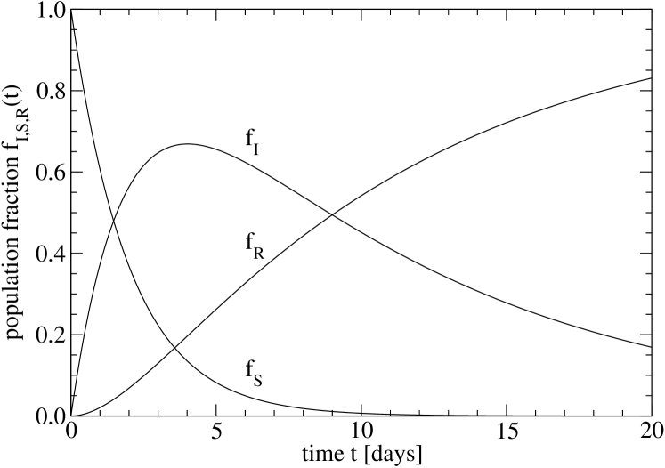
Figure 1: An example of a solution of the SIR equations (9), starting with the initial conditions that the fraction of susceptibles is $f_{\rm S}=1.0$ (all), and the infection rate $r_{\rm I}=0.5$ [days^-1] is five times the recovery rate, $r_{\rm R}=0.1$ [days^-1].

The behavior of this system is just what one would expect from the dynamics described in the SIR-type defining equations (5): The initial population of susceptibles ($\rm S$) decays exponentially at the specified rate $r_{\rm I}$ as they transition into infected ($\rm I$); the infected fraction increases to a maximum fI_max , and then declines as it populates the final, recovered population ($\rm R$). As $t\to\infty$ one asymptotically approaches a state in which all of the population has transitioned to recovered, $f_{\rm R}(t=+\infty)=1$. As anticipated, at any intermediate time $0<t<+\infty$, $f_{\rm S}(t)+f_{\rm I}(t)+f_{\rm I}(t)=1$.

As a specific example, the time dependence predicted by this SIR model is shown in Fig.1, for $r_{\rm I}=0.5$ [days^-1] and $r_{\rm R}=0.1$ [days^-1] (an infection rate of five times the recovery rate).

I.2 A “SHIR” Model for COVID-19

Two important modifications to this simple pedagogical SIR model appear appropriate for a more realistic description of the COVID-19 pandemic. One is that the rate of transitions from susceptible (S) to infected (I) should be proportional to the product of these two populations, since their interaction determines this rate. This modifies the second evolution equation for the population fraction $f_{\rm I}(t)$ to

$$df_{\rm I}/dt=+r_{\rm I}f_{\rm S}f_{\rm I}-r_{\rm R}f_{\rm I}\ .$$ (15)

This “second-order reaction kinetics” in the infection process is a standard assumption in epidemic models Roc2014 ; Ker1927 .

A second, more novel modification of the SIR model is to incorporate the effects of a social response to a high-profile pandemic such as COVID-19. In this case there has been strong encouragement from governments and medical authorities to reduce the growth of the pandemic by implementing social distancing and related measures. In this SHIR model these actions reduce the susceptible population by transferring them to a new category of “hidden” individuals (H) who are not susceptible to infection, which is populated from the original group of susceptibles (S) through another rate process,

$$df_{\rm H}/dt=+r_{\rm H}f_{\rm S}\ .$$ (16)

The individuals in ${\rm H}$ are not only the physically sequestered; simply changing behavior, such as avoiding public assemblies, crowded schools and public transportation, implementing rigorous hygienic practices, and many other measures contribute to the continued reduction of the effective susceptible population fraction $f_{\rm S}$ Hbox .

We consider $\tau=1/r_{\rm H}$, the “social response time,” to be a measure of how quickly a society responds to a developing pandemic threat. We shall subsequently find that there are interesting differences between countries in the fitted values of this parameter.

The partner DE for $f_{\rm S}$, similarly modified to include a second-order infection rate process as well as the new first-order social response transition term for ${\rm S}\to{\rm H}$, is

$$df_{\rm S}/dt=-r_{\rm I}f_{\rm S}f_{\rm I}-r_{\rm H}f_{\rm S}\ .$$ (17)

The final “recovery” DE for $d{\rm R}/dt$ is unchanged from the SIR model formula in (5). However since the ${\rm R}$ cases in practice include mortality as well as recovery, we will instead refer to the ${\rm R}$ population as “resolved” Ard .

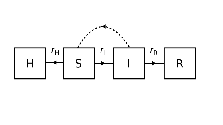
Figure 2: A block diagram of the “SHIR” model, which generalizes SIR by introducing a “hidden” population H and an ${{\rm S}\to{\rm H}}$ rate constant $r_{\rm H}$.

Collecting these results gives our complete set of SHIR model DEs,

$$df_{\rm H}/dt =+r_{\rm H}f_{\rm S}$$ (18)

$$df_{\rm S}/dt =-r_{\rm I}f_{\rm S}f_{\rm I}-r_{\rm H}f_{\rm S}$$ (20)

$$df_{\rm I}/dt =+r_{\rm I}f_{\rm S}f_{\rm I}-r_{\rm R}f_{\rm I}$$ (22)

$$df_{\rm R}/dt =+r_{\rm R}f_{\rm I}\ .$$ (24)

Note that one recovers the three original pandemic DEs of Kermack et al. Ker1927 (their Eqs.(29)) through the substitutions $f_{(\rm S,\rm I,\rm R)}\to(x,y,z)/{\rm N}$ and $(r_{\rm I},r_{\rm R})\to(\kappa,\ell)$, and removing the “hidden population” of the SHIR model by setting $r_{\rm H}=0$ and $f_{\rm H}=0$.

We note in passing that the infected (and still infective) individuals (all those in box ${\rm I}$) are also referred to in the literature as the “active” cases, numbering ${\rm A}(t)$. Here, ${\rm I}(t)$ and ${\rm A}(t)$ are identical; any individuals in box ${\rm I}$ who are no longer infective are immediately reclassified as “resolved,” and moved to box R.

Since (24) is a nonlinear set of ODEs for the four population fractions $f_{\rm S,\rm H,\rm I,\rm R}$, an exact analytical solution will not be possible, except in certain limits and approximations. However some important results can still be proven for this nonlinear system. One such result, obtained by adding the 4 equations in (24), is that the sum of the four populations fractions $f$ is a constant of motion. Thus $f_{\rm H}+f_{\rm S}+f_{\rm I}+f_{\rm R}=1$, or ${\rm H+\rm S+\rm I+\rm R}$ remains a constant, ${\rm N}_{0}$.

Another useful result is that the population fractions of the two groups H “hidden” and R “resolved” can be expressed simply in terms of the susceptible (S) and infected (I) fractions $f_{\rm S}$ and $f_{\rm I}$,

$$f_{\rm H}(t)=f_{\rm H}(t_{0})+r_{\rm H}\int_{t_{0}}^{t}f_{\rm S}(t^{\prime})dt^{\prime}$$ (25)

and

$$f_{\rm R}(t)=f_{\rm R}(t_{0})+r_{\rm R}\int_{t_{0}}^{t}f_{\rm I}(t^{\prime})dt^{\prime}\ .$$ (26)

Our principle task will therefore be to solve the two coupled equations for $f_{\rm S}(t)$ and $f_{\rm I}(t)$, the second and third equations in the set (24).

Since the rate of increase of the infected fraction $df_{\rm I}/dt$ is proportional to the product $f_{\rm I}f_{\rm S}$, a trivial solution of the model follows from an initial condition of no infections, $f_{\rm I}(t=0)=0$; this implies $f_{\rm I}(t)=0$, i.e. that there are no infections at any later (or earlier) time. In this limit all that happens is that the initial fully susceptible population $f_{\rm S}(t=0)=1$; $f_{\rm H}(t=0)=0$ evolves into an increasingly hidden population, as a decaying exponential;

$$f_{\rm S}(t) =e^{-r_{\rm H}t}\ ,$$ (27)

$$f_{\rm H}(t) =1-e^{-r_{\rm H}t}\ .$$ (29)

In practice the fraction of infected individuals $f_{\rm I}(t)$ will usually be much smaller than the fraction of susceptibles $f_{\rm S}(t)$. This suggests that we use the no-infection limit (29) for $f_{\rm S}(t)$ as a first approximation in determining $f_{\rm I}(t)$ in the small-$f_{\rm I}(t)$ limit. With this substitution, we find that the increase in $df_{\rm I}/dt$, the fractional rate of new cases per day, will be

$$\lim_{{\rm S}>>{\rm I}}df^{(in)}_{\rm I}/dt=+r_{\rm I}e^{-r_{\rm H}t}f_{\rm I}\ .$$ (30)

For completeness we note that the rate of decrease of the “active” (still infective) population fraction $f_{\rm I}(t)$ per day due to transitions from “infected” to “resolved” status is given by

$$df^{(out)}_{\rm I}/dt=-r_{\rm R}f_{\rm I}$$ (31)

so the full DE for $f_{\rm I}(t)$ in this small-$f_{\rm I}(t)$ limit is

$$\lim_{{\rm S}>>{\rm I}}df_{\rm I}/dt=+(r_{\rm I}e^{-r_{\rm H}t}-r_{\rm R})f_{\rm I}\ .$$ (32)

The formula for the fractional “new cases per day” (cpd) growth rate in the small-$f_{\rm I}(t)$ approximation, Eq.(30), is attractive for several reasons. First, it is easily compared to data, since there is copious information available from many countries regarding the number of new cases per day. (This quantity is simply ${\rm N}_{0}$ times the $df^{(in)}_{\rm I}/dt$ above.) Second, since (32) is a linear, homogeneous, first-order differential equation involving only $f_{\rm I}(t)$, and the associated integral over time is tractable, we may solve for $f_{\rm I}(t)$ analytically in this small-$f_{\rm I}(t)$ approximation.

In the early and intermediate stages of a pandemic in which the infected fraction still dominates the resolved fraction, we can ignore the assumed slower transition of infected to resolved by setting $r_{\rm R}=0$, which gives

$$\lim_{{\rm S}>>{\rm I}>>{\rm R}}df_{\rm I}/dt=+r_{\rm I}e^{-r_{\rm H}t}f_{\rm I}\ .$$ (33)

This relation is especially amenable to comparison with data, as it relates two observed quantities, the number of new cases per day (${\rm N}_{0}df_{\rm I}(t)/dt$) and the cumulative number of cases (${\rm N}_{0}f_{\rm I}(t)$), assuming that ${\rm N}_{0}f_{\rm R}(t)$ can be neglected. The SHIR model in this small-infected-fraction limit predicts that this ratio should be a decaying exponential in time,

$$\lim_{{\rm S}>>{\rm I}>>{\rm R}}\frac{df_{\rm I}/dt}{f_{\rm I}}=+r_{\rm I}e^{-r_{\rm H}t}\ .$$ (34)

In the following section we will compare the expected time dependence of several pandemic models to COVID-19 data, including the SHIR model prediction (34). We will follow this with more detailed SHIR-model calculations of the cumulative case numbers ${\rm N}_{0}f_{\rm I}(t)$ and especially the new cases per day (cpd), ${\rm N}_{0}df_{\rm I}(t)/dt$, and will describe detailed fits of these functions to COVID-19 data from a range of countries.

II Pandemic Dynamics

II.1 Simple models versus COVID-19 data

Here we will first discuss the time dependence predicted by two familiar dynamic models of pandemics, and will show how these models can be compared to COVID-19 data. We will find that there are serious difficulties in applying these simple models to COVID-19.

In this discussion we will consider only the cumulative number of cases as a function of time (here called ${\rm P}(t)$), and the rate of appearance of new cases per day, $d{\rm P}/dt$. These numbers are widely reported for COVID-19, and require little interpretation. One important point is that the number of cumulative cases to time $t$, ${\rm P}(t)$, is the sum of the infected ${\rm I}(t)$ and the resolved ${\rm R}(t)$ populations distinguished in the previous section;

$${\rm P}={\rm I}+{\rm R}\ .$$ (35)

As a first, simplest model of the growth of a pandemic, one can assume that the rate of change of the number of cases $d{\rm P}/dt$ is proportional to the number of cases ${\rm P}$,

$$\frac{d{\rm P}}{dt}\equiv\dot{\rm P}=\lambda{\rm P}\ .$$ (36)

The solution of this differential equation is an exponential times the number of cases at some arbitrary initial time,

$${\rm P}(t)={\rm P}(0)\;e^{\lambda t}\ .$$ (37)

This simple model clearly makes unrealistic assumptions, notably that there are infinitely many potential cases. It also neglects spatial dependence or other “local” aspects of the problem, as well as the effect of transitions from infected to resolved individuals who are no longer infective. This exponential model predicts that the ratio of new cases per day to cumulative cases should be a constant,

$$\frac{d{\rm P}/dt}{\rm P}=\lambda\ .$$ (38)

In Fig.3 we compare this expectation to the ratio of new cases reported per day ($\Delta{\rm P}/\Delta t$) to the cumulative number of cases (${\rm P})$ for the UK, using data from Ref.WCU over the period 18 Mar - 04 May 2020. Evidently this ratio is far from constant; it falls by about a factor of 10 over the 47-day period shown.

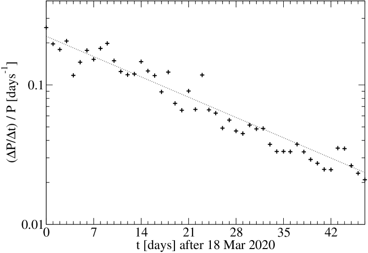
Figure 3: The ratio of new cases per day to cumulative cases in UK COVID-19 data. The exponential model prediction of a constant ratio (38) evidently disagrees strongly with this data. The dotted line shows an alternative fit to a decaying exponential, which appears as a straight line on this log/linear plot.

The simple exponential model can be improved through the introduction of a limit in the number of the population that can be infected, ${\rm P}_{max}$. One can assume that the infection rate is initially equivalent to the exponential model, but later in the pandemic is suppressed in proportion to the number of uninfected individuals remaining, ${\rm P}_{max}-{\rm P}$. A simple DE with these properties is the “logistic model,” defined by

$$\frac{d{\rm P}}{dt}=\lambda{\rm P}(1-{\rm P}/{\rm P}_{max})\ .$$ (39)

The solution of this model, which is symmetric about ${\rm P}={\rm P}_{max}/2$, is the inverse of an exponential plus a constant, translated by a $t_{0}$ that is determined by the initial conditions;

$${\rm P}(t)=\frac{{\rm P}_{max}}{\big{(}1+e^{-\lambda(t-t_{0})}\big{)}}\ .$$ (40)

This logistic model can also easily be tested by comparison with data on the ratio of new cases per day to cumulative cases. In this case, the model predicts that this ratio should be a simple, linear function of ${\rm P}$,

$$\frac{d{\rm P}/dt}{\rm P}=\lambda(1-{\rm P}/{\rm P}_{max})\ .$$ (41)

So, when data on this ratio (y-axis) is plotted against ${\rm P}$ (x-axis), this model anticipates linear ${\rm P}$-dependence, with an x-axis intercept (where $d{\rm P}/dt=0$) at ${\rm P}={\rm P}_{max}$.

In Fig.4 we show an example of this plot for COVID-19 data, using the USA cumulative cases and new cases per day data from Ref.WCU through 15 July 2020. Although this ratio initially has some qualitative resemblance to the logistic model form (41), (see Fig.4 upper left), the more recent data (lower right) is clearly inconsistent with (41), and cannot be extrapolated linearly to zero $d{\rm P}/dt$.

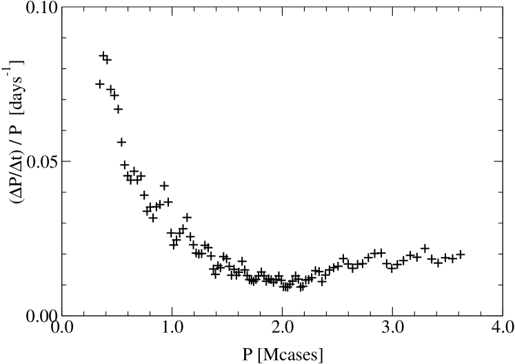
Figure 4: The ratio of new cases per day to cumulative cases in USA COVID-19 data (y-axis), plotted against total cumulative cases (x-axis).

A study of the pandemic time dependence predicted by the logistic model shows another specific aspect of the model that makes it unrealistic for COVID-19; the rate of new cases $d{\rm P}/dt$ predicted by this model is symmetric about the maximum, at the ${\rm P}(t)$ inflection point $t=t_{0}$. We shall see that in contrast the rate of new cases $d{\rm P}/dt$ observed in the COVID-19 data is rather skewed, and has a faster rise to maximum than the subsequent decline.

II.2 The SHIR model versus COVID-19 data

Here we will test a third prediction for time dependence, which is the form predicted by the SHIR model of the previous section. There we noted that the infected fraction ${f_{\rm I}}$ of the population is predicted to satisfy the differential equation

$$\frac{df_{\rm I}/dt}{f_{\rm I}}=+r_{\rm I}e^{-r_{\rm H}t}$$ (42)

in the limits of a small fraction of the population being infected (${f_{\rm I}}<<1$) and the resolved fraction being small relative to the infected fraction (${f_{\rm R}}<<f_{\rm I}$). The existing COVID-19 data suggests that these are both reasonable approximations in the early and intermediate stages of the COVID-19 pandemic.

The expectation (42) can immediately be compared to data, since $(df_{\rm I}/dt)/f_{\rm I}$ is just the ratio shown on the y-axis of Fig.3. The dotted line in the figure shows a decaying exponential fit of exactly the form (42), which evidently gives a very good description of the data. The parameter values found in this fit are $r_{\rm I}=0.233$ [days^-1] and $\tau\equiv 1/r_{\rm H}=20.9$ [days].

Motivated by the good agreement between the SHIR model prediction of a decaying exponential in time for $(df_{\rm I}/dt)/f_{\rm I}$ and the COVID-19 data evident in Fig.3, we will subsequently discuss SHIR model predictions in more detail, and will show fits of this model to COVID-19 data from many European countries. This will follow a short discussion of some general aspects of mathematically similar models, which will be used in the detailed discussion of SHIR results.

II.3 General results for a class of pandemic models

The results discussed above motivate the consideration of generalizations of the simplest “pure exponential” pandemic model, in which the constant $\lambda$ of that model (38) is replaced by an explicit function of time,

$$\frac{d{\rm P}/dt}{\rm P}\equiv\lambda(t)\ .$$ (43)

For a given function $\lambda(t)$, the defining differential equation (43) gives the predicted growth of case numbers as

$${\rm P}(t)={\rm P}(0)\;e^{\int_{0}^{t}\lambda(t^{\prime})dt^{\prime}}.$$ (44)

Formally this may be regarded as exponential growth in a new (nonlinear) time variable $u$, defined by $du=\lambda(t)dt$.

Since this is a model of the growth of a pandemic, the cumulative number of cases (44) can only increase, or become flat when the pandemic has been completely halted, which occurs if and when we reach a time $t_{f}$ for which $\lambda(t_{f})=0$. Accordingly we constrain $\lambda(t)$ to be positive (pandemic ongoing, $t<t_{f}$) or zero ($t=t_{f}$, pandemic halted).

The inflection point of ${\rm P}(t)$ is of considerable importance, since this is the time of peak pandemic growth. The time $t_{infl}$ of the inflection point is specified by the rate of change of case numbers $d{\rm P}/dt$ reaching a maximum; this occurs when the second derivative $d^{2}{\rm P}/dt^{2}$ is zero,

$$\frac{d^{2}{\rm P}(t)}{dt^{2}}\Big{|}_{t=t_{infl}}=0\ .$$ (45)

On substituting the general solution ${\rm P}(t)$ from (44) into this constraint, we find an equivalent definition of the inflection point in terms of the proportional growth function $\lambda(t)$,

$$\Bigg{\{}\frac{d\lambda(t)}{dt}+\lambda(t)^{2}\Bigg{\}}\Bigg{|}_{t=t_{infl}}=0\ .$$ (46)

III Predictions of the SHIR model

III.1 Cumulative cases ${\rm P}(t)$ and cases per day (cpd) $d{\rm P}/dt(t)$

In Sec.I.B. we introduced the “SHIR” model as a generalization of the SIR model, with the effects of pandemic reduction measures incorporated through a “hidden” population (H) that migrates from the initial susceptible population (S) with a rate constant $r_{\rm H}$. In the limit of a small infected population fraction ($f_{\rm I}<<1$) relative to the remaining fraction of susceptibles ($f_{\rm S}$), and assuming that the resolved fraction $f_{\rm R}$ can be neglected, we showed that the infected fraction satisfies a differential equation of the form

$$\lim_{{\rm S}>>{\rm I}>>{\rm R}}\frac{df_{\rm I}/dt}{f_{\rm I}}=\lambda(t)$$ (47)

where the SHIR growth rate function is a decaying exponential in time,

$$\lambda(t)=+r_{\rm I}e^{-r_{\rm H}t}\ .$$ (48)

The rate coefficients $r_{\rm H}$ and $r_{\rm I}$ can be interpreted respectively as a characteristic “social response time” $\tau=1/r_{\rm H}$ for the implementation of pandemic reduction measures, and an initial condition (at some $t=0$) on the growth rate function $\lambda(t)$;

$$\lambda(t)=\lambda(0)\,e^{-t/\tau}\ .$$ (49)

If we multiply the infected fraction $f_{\rm I}$ by the total population ${\rm N}_{0}$,

$${\rm P}(t)={\rm N}_{0}\cdot f_{\rm I}$$ (50)

and similarly scale the fractional new cases per day,

$$d{\rm P}/dt={\rm N}_{0}\cdot df_{\rm I}/dt\;,$$ (51)

we can compare the results for the cumulative cases ${\rm P}(t)$ and new cases per day $d{\rm P}/dt$ directly to the data as normally reported.

Given the form (49), on solving (47) we find that the predicted number of cases as a function of time in the SHIR model is a nested exponential,

$${\rm P}(t)={\rm P}_{max}/\exp\big{(}\lambda(0)\tau\,e^{-t/\tau}\big{)}.$$ (52)

This may be simplified by replacing the $t=0$ initial condition $\lambda(0)$ by an equivalent time shift

$$t_{0}=\tau\ln(\lambda(0)\tau)\ ,$$ (53)

which gives a simple three-parameter form for the general solution of the cumulative number of cases in the SHIR model,

$${\rm P}(t)={\rm P}_{max}/\exp\big{(}e^{-(t-t_{0})/\tau}\big{)}.$$ (54)

This function increases monotonically from ${\rm P}=0$ at $t=-\infty$ to ${\rm P}_{max}$ at $t=+\infty$, and has a single inflection point at $t=t_{0}$. This is an example of a Gompertz Gom1832 curve, $y=ab^{q^{x}}$Wei ; these are often encountered in problems in which a proportional rate of growth $\dot{f}/f$ is driven by an exponential.

The rate of appearance of new cases per day (cpd) in the model, $d{\rm P}/dt$, can be evaluated directly from ${\rm P}(t)$ above, and is

$$\frac{d{\rm P}}{dt}=\frac{{\rm P}_{max}}{\tau}\cdot e^{-(t-t_{0})/\tau}/\exp\big{(}e^{-(t-t_{0})/\tau}\big{)}.$$ (55)

This rate of growth is zero at $t=-\infty$, increases to a maximum value at the ${\rm P}(t)$ inflection point $t_{0}$, and then decreases with time, approaching zero exponentially as $t\to+\infty$. $d{\rm P}/dt$ integrates to a finite number of cases ${\rm P}_{max}$ as $t\to+\infty$. The maximum number of cases per day, at the time $t_{0}$ of the ${\rm P}(t)$ inflection point, is given by

$$\frac{d{\rm P}}{dt}\bigg{|}_{t=t_{infl}=t_{0}}=\frac{{\rm P}_{max}}{e\tau}\ .$$ (56)

The three parameters that specify a solution of the SHIR model, ${\rm P}_{max}$, $\tau$ and $t_{0}$, all have simple interpretations; they are respectively the height, width scale, and time shift of the pandemic profile ${\rm P}(t)$ (or of the rate of new cases, $d{\rm P}/dt$). ${\rm P}_{max}$ is by definition the maximum value of ${\rm P}(t)$, and gives the total number of cases, which is ${\rm P}(t)$ at $t=+\infty$. The social response time $\tau$ sets the scale for all time-interval features of ${\rm P}(t)$ and $d{\rm P}/dt$, since changing $t_{0}$ only translates these functions. The time shift $t_{0}$ is the time of the inflection point of ${\rm P}(t)$,

$$t_{infl}=t_{0}=\tau\ln(\lambda(0)\tau).$$ (57)

This inflection point $t_{0}$ may be considered the peak of the local pandemic, since the number of new cases per day estimated by the fit is then a maximum.

For discussion purposes a convenient choice for $t_{0}$ in (54) and (55) is $t_{0}=0$, which places the inflection point of ${\rm P}(t)$ at $t=0$. Plotting ${\rm P}(t)$ or $d{\rm P}/dt$ against $t$ in units of $\tau$, normalized to their maximum values, gives a parameter-independent “universal profile” for each of these functions. The universal form for ${\rm P}(t)$, scaled by its maximum value ${\rm P}_{max}$, is shown in Fig.5. The inflection point of ${\rm P}(t)$ at $t=0$ is indicated, where both ${\rm P}(0)/{\rm P}_{max}$ and its slope (in the dimensionless time variable $t/\tau$) equal $e^{-1}$. This last property implies that the total number of cases ${\rm P}_{max}$ and the cumulative number of cases at the time of the ${\rm P}(t)$ inflection point (pandemic maximum), ${\rm P}(t_{0})$, are related by

$${\rm P}_{max}=e\cdot{\rm P}(t_{0})\ .$$ (58)

This provides a simple estimate of the total expected cases ${\rm P}_{max}$ from the number observed up to the pandemic peak, ${\rm P}(t_{0})$, which may already be known.

Some additional times of interest are those at which ${\rm P}(t)$ has reached $10\%$, $50\%$, $90\%$ and $99\%$ of the total cumulative cases; these are respectively $(t-t_{0})/\tau=-0.8340,+0.3665,+2.250,$ and $+4.600$.

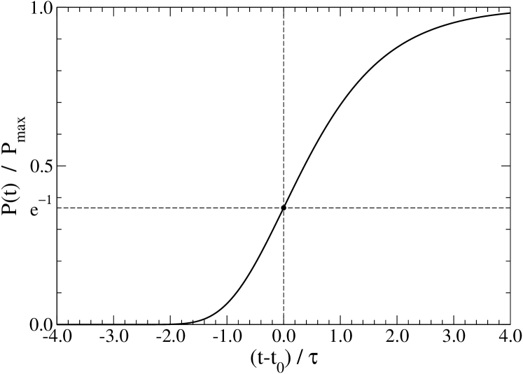
Figure 5: A “universal” plot of the cumulative case numbers ${\rm P}(t)$ predicted by the SHIR model (54). To the extent that the model is accurate, all cumulative case number data should follow this curve.

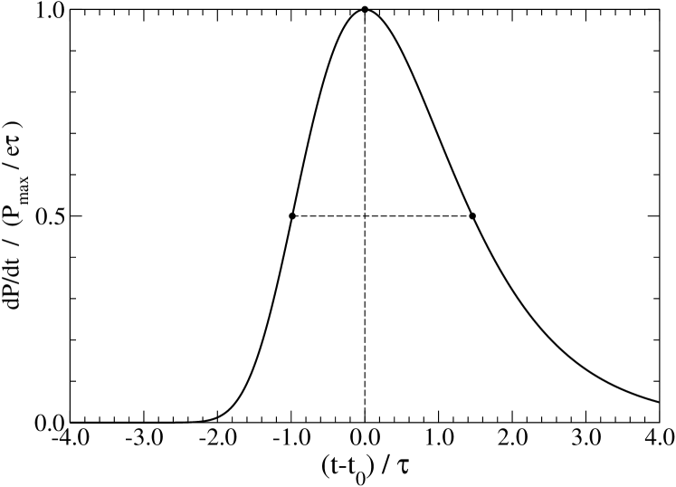
Figure 6: The corresponding universal plot of new cases per day (cpd), $d{\rm P}/dt$, predicted by the SHIR model (55). The cpd data should follow this curve if the SHIR model is accurate.

The universal curve for $d{\rm P}/dt$, the new cases per day, is shown in Fig.6, scaled by its maximum value of ${\rm P}_{max}/e\tau$. The mean and variance of $t$ for this distribution are $<t>=\gamma\tau$ ($\gamma$ is Euler’s constant) and $\sigma=(\pi/\sqrt{6})\tau$. The skewness def_skewness of $d{\rm P}/dt$ is $12\sqrt{6}\,\zeta(3)/\pi^{3}\approx+1.140$, a positive value indicating a more heavily weighted RHS. Several additional interesting features of $d{\rm P}/dt$ are the FWHM, $2.446\tau$ (indicated in Fig.6), the rise time of $d{\rm P}/dt$ from half-max to peak, which is $0.985\tau$; and the much slower decline of $d{\rm P}/dt$ from peak to half-max, which requires $1.461\tau$.

The asymptotic approach of ${\rm P}(t)$ to ${\rm P}_{max}$ cases at large times is exponential,

$$\lim_{t\to\infty}{\rm P}(t)/{\rm P}_{max}=1-e^{-(t-t_{0})/\tau},$$ (59)

as is the (decreasing) rate of growth of new cases at large times,

$$\lim_{t\to\infty}\frac{d{\rm P}}{dt}=({\rm P}_{max}/\tau)\,e^{-(t-t_{0})/\tau}\ .$$ (60)

We note in passing that these results suggest an improved estimate of the asymptotic total number of cases ${\rm P}_{max}$ which has accelerated convergence,

$$\lim_{t\to\infty}\Big{(}{\rm P}(t)+\tau\frac{d{\rm P}}{dt}\Big{)}={\rm P}_{max}+O(e^{-2(t-t_{0})/\tau}),$$ (61)

although this improved behavior would likely be masked in practice by the background of sporadic cases.

IV Application of the SHIR model to COVID-19 Data

IV.1 Goals of the Fitting Exercise

In this section we will show results from fitting the predicted early pandemic time dependence from the SHIR model as derived in Sec.IIIA to data for the confirmed COVID-19 case numbers from many different countries. We will primarily consider fits of the new case numbers per day (cpd) to the SHIR model prediction, Eq.(55). As an initial example we will show results for Austria, including fits to both the cpd and the cumulative case numbers. Following this we will give the results of SHIR model fits to the cpds reported by a representative set of Western countries, and will compare and contrast these results. We will also discuss procedures for fitting more complicated datasets that show evidence for multiple infection sites, and will show examples of such fits. Finally we will show how datasets from multiple countries can be combined, and will use this procedure to test the predicted SHIR model profile for new cases per day, displayed as a universal (parameter-free) curve.

IV.2 SHIR model single country fits: Europe

As a first application we will fit the three-parameter SHIR model to the data on the number of new daily COVID-19 cases per day in Austria, as reported on the Worldometer website, Ref.WCU . Austria was chosen because it represents one of the earliest COVID-19 outbreaks in Europe, so their data allows us to follow both the earlier and later stages of the pandemic. For this fit we will use the entire Austrian cpd dataset from the initial website date of 15 Feb 2020 through 06 May 2020, comprising a nominal 82 data points. (For most countries we consider, including Austria, there are actually many “null” or zero entries in the early dates.)

As a reminder, in the small fraction of infections limit assumed here one may solve the model for the cumulative case numbers of infected people ${\rm P}(t)$ and hence the rate of new cases per day $d{\rm P}/dt$ in closed form, given by Eqs.(54,55). The three free parameters in these functions are ${\rm P}_{max}$ (total number of cases), $\tau$ (social response time), and $t_{0}$ (the ${\rm P}(t)$ inflection point; time of the maximum cases per day). Our common $t=0$ reference time in all these numerical fits and discussions is taken to be 18 Mar 2020. The fits are all simple, unweighted least-squares without data errors.

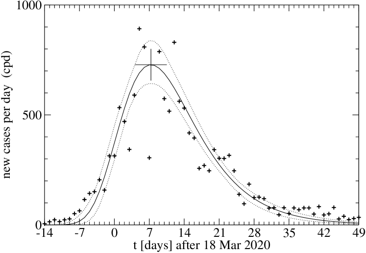
Figure 7: New COVID-19 cases per day reported for Austria over the period 15 Feb - 06 May 2020, with a SHIR model fit (solid line). The maximum new case rate and associated time (the ${\rm P}(t)$ inflection point, $t_{0}$) in the model are indicated by a single large point. Estimated 95% CL limits are shown as dotted lines.

The result of this fit for Austria is shown in Fig.7. This is a surprisingly good fit to the full range of the cpd data, including the rapid initial rise after the early cases, the peak region, and the subsequent slower decline; all are reasonably well described by the model AusNorWCUpts .

The SHIR model parameters resulting from this fit to the cpd data from Austria are given below.

$${\rm P}_{max} =14.9(8)k\ [\hbox{\rm cases}]$$ (62)

$$\tau =7.54(50)\ [\hbox{\rm days}]$$ (63)

$$t_{0} =7.32(49)\ [\hbox{\rm days}]\ .$$ (64)

These and other fitted parameters are typically quoted to three-place accuracy in this paper, to allow numerical tests such as debugging of numerical routines and checking analytic results.

There is evidently reasonable agreement between the SHIR model and the data with these parameters for the number of new cases per day, although there is considerable scatter in the data. The numerical value of the peak predicted cpd, ${\rm P}_{max}/e\tau$, and the time of the peak, $t_{infl}=t_{0}$ are indicated by a single large point in Fig.7. These values are respectively 728 [cases/day] and 7.32 [days] (measured from $t=0$ on 18 Mar 2020), giving 25 Mar 2020 as the peak date for new cases per day in Austria implied by this fit.

The fitted value of the Austrian “social response time,” $\tau\approx 7.5$ [days], is of special note. This is the smallest value (hence the fastest social response) we have found in our fits to the COVID-19 pandemic numbers from a large set of 15 representative Central and Western European countries (see Table 1). This suggests that Austria deployed an especially rapid and effective response to this pandemic, which presumably had a strongly limiting effect on the total number of cases.

A minor discrepancy between the model and data is evident at the early times in Fig.7 that are characterized by small case numbers. (See times before about $t=-4$ [days] in the figure.) The number of early cases is clearly underpredicted by the fit. This may represent their growth from a small number of initial cases, closely monitored and hence developing rather slowly, which were evident before the primary pandemic contribution became dominant. We will note a similar, more prominent effect in the early data from Denmark and Norway at about the same date.

An alternative approach would be to fit the cumulative number of reported cases as a function of time, which is typically reported together with the new cases per day. Since one is the derivative of the other, these should give similar parameter values. Of course the results will not be identical, because the model is not exact, and the cumulative cases data will give higher fitting weight to the later stages of the pandemic.

The choice of which dataset to fit, cumulative cases or new cases per day, may be suggested by the subject of greatest interest; the peak of the pandemic is best determined by fitting the new cases per day, but the final number of cases will be best determined if constrained by the large total case numbers reported in the later stages of the pandemic.

Here as an example of the second fit we give the SHIR model results that follow from fitting the cumulative case numbers from Austria. We again use a set of 82 points of Austrian data WCU from the initial reporting date of 15 Feb 2020 through the fitting date, 06 May 2020. The SHIR model fit to the Austrian cumulative cases data is shown in Fig.8. The parameters resulting from this cumulative cases fit are

$${\rm P}_{max} =15.54(5)k\ [\hbox{\rm cases}]$$ (65)

$$\tau =8.18(11)\ [\hbox{\rm days}]$$ (66)

$$t_{0} =6.53(7)\ [\hbox{\rm days}]$$ (67)

Evidently the SHIR model also provides a reasonably accurate description of the cumulative cases for Austria.

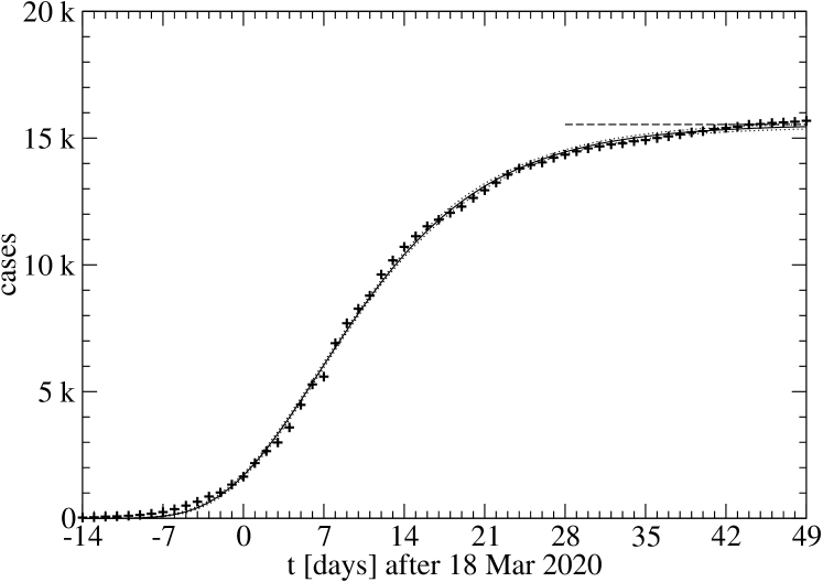
Figure 8: A fit of the SHIR model to Austrian cumulative COVID-19 cases, showing the data and the corresponding model results for ${\rm P}(t)$ (solid line). Estimated 95% CL limits are included as dotted lines, but are very close to the central curve. The asymptotic number of cases predicted by this fit, $15.54k$, is shown as a horizontal dashed line.

The parameter values resulting from the two fits, to cpd data (64) and cumulative cases data (67), are quite similar cas_fit . The total case numbers ${\rm P}_{max}$ differ from their mean by $\pm 2\%$, the fitted social response times $\tau$ differ from their mean by $\pm 4\%$, and the fitted times of the Austrian inflection point (maximum rate of new cases) in the two fits differ by just 0.8 [days].

Next we will follow the same procedure described in the first Austrian fit above, and will fit the SHIR model to the cpd data for each of a representative set of Central and Western European countries. For each fit, as discussed for Austria, we have again used 82 pts of daily new case numbers per day WCU for the period 15 Feb - 06 May 2020 as the only input data. This data fitted to the three-parameter SHIR model form for $d{\rm P}(t)/dt$, (55). This fixes the three model parameters ${\rm P}_{max}$ (with units of [cases]), $\tau$ [days], and the inflection point $t_{infl}=t_{0}$ [days] (measured from $t=0$ on 18 Mar 2020) separately for each country.

The fitted parameter values for the entire set of 15 Central and Western European countries considered here are given in Table.1, together with the calendar date of the inflection point $t_{0}$, and the fitted peak number of new cases per day, which occurs at $t_{0}$.

Country	${\rm P}_{max}$	$\tau$	$t_{0}$	peak date	max cpd
Austria	14.9$k$	7.54	7.32	25 Mar	0728
Iceland	1.80$k$	8.69	7.55	26 Mar	0076
Switzerland	30.2$k$	10.1	8.02	26 Mar	1100
Norway∗	6.95$k$	10.1	8.71	27 Mar	0252
France	175$k$	10.5	16.3	03 Apr	6100
Germany	172$k$	11.3	12.0	30 Mar	5590
Ireland	24.0$k$	11.8	26.2	13 Apr	0750
Portugal	28.6$k$	13.2	17.6	05 Apr	0599
Belgium	57.4$k$	14.2	19.8	07 Apr	1491
Spain	273$k$	14.2	14.4	01 Apr	7010
Denmark∗	10.2$k$	14.3	19.6	07 Apr	0262
Netherlands	46.9$k$	15.2	18.0	05 Apr	1140
Italy	232$k$	16.1	9.72	28 Mar	5310
UK	302$k$	20.4	30.9	18 Apr	5450
Sweden	40.9$k$	25.7	33.8	21 Apr	0586

Table 1: The result of fitting the SHIR model to the data on COVID-19 new cases per day from 15 representative Central and Western European countries. The first two model parameters shown are the predicted total cumulative COVID-19 cases ${\rm P}_{max}$ and the social response time $\tau$. The entries are ordered by $\tau$. The final three columns give the fitted inflection point $t_{0}$ (the pandemic peak) [days after 18 Mar 2020] and date, and the fitted maximum cpd (at $t_{0}$).      ^∗See discussion.

IV.3 Implications of European Single Country Fits

Perhaps the most remarkable aspect of the SHIR model fits to 15 Central and Western European countries in Table.1 is the wide range of values found for the “social response time” $\tau$, and how it appears to correlate with national coronavirus policy. As $\tau$ sets the width of the pandemic peak, it is a measure of how long a country will have to endure the pandemic. (Recall for example that the FWHM of the new cases per day, $d{\rm P}/dt$, is about $2.4\cdot\tau$.) The extreme cases are Austria ($\tau\approx 7.5$ days) and Sweden ($\tau\approx 26$ days), over 3 times longer than Austria. The Swedish cpd data and fit are shown in Fig.9.

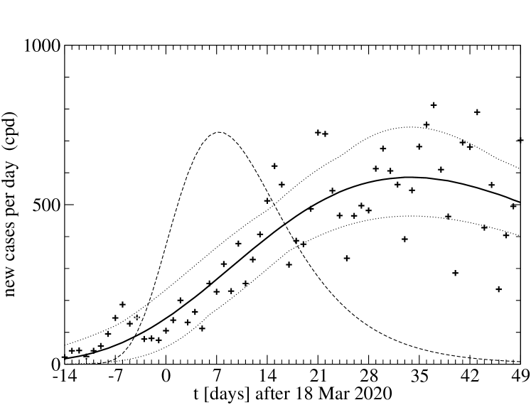
Figure 9: The SHIR model fit to the Swedish COVID-19 new cases per day data over the period 15 Feb - 06 May 2020. Estimated 95% CL limits are shown as dotted lines. The corresponding fit to the Austrian cpd data of Fig.7 is shown for comparison as a dashed line.

The very slow Swedish response time is apparently the result of a rather controversial COVID-19 policy promoted by the Swedish State Epidemiologist, A. Tegnell Sweden_policy , which did not impose the strict school closings, border controls, and restrictions on large gatherings that characterized the policies of other Scandinavian countries. Tegnell instead advocated a more open society during the pandemic, to promote herd immunity and a quick economic recovery. Although the Swedish policy was evidently successful in broadening the curve, their per capita number of cases is over twice that of Denmark and Norway, and the Swedish fatalities per capita are larger by a similar amount. This argues that an aggressive national policy of minimizing the social response time $\tau$, for example through contact tracing, extensive testing, rapid medical response and isolation of positive cases through quarantine, may be the most effective in reducing the total case and fatality numbers. It may also prove easier to sustain a strict policy over a short period of time than a more lax one over a longer period.

The UK and Dutch social response times $\tau$ are also quite large, and can also be correlated with their early national policies that promoted “flattening the curve” and developing herd immunity. To quote the Dutch Prime Minister regarding COVID-19 policy in a national address Netherlands_policy , (in translation) “… we can slow down the spread of the virus while at the same time building group immunity in a controlled way.” In a national address UK_policy the UK Prime Minister stated that “It is vital to slow the spread of the disease. That is the way we reduce the number of people needing hospital treatment at any one time.”

Of course the argument that slowing the spread of the pandemic is advantageous because it “flattens the curve” is specious. This tacitly assumes that the total number of cases ${\rm P}_{max}$ is constant, so a broader rate curve must have a lower mean. In practice there is instead evidence that a longer $\tau$ may result in more infections per capita, as seen in comparing Sweden with Denmark and Norway. If so, flattening the curve by slowing the spread of the pandemic unfortunately increases the total number of cases and fatalities. This complicated and perhaps counterintuitive issue certainly merits careful future investigation.

IV.4 SHIR model single country fits: North America

We have also carried out fits of the SHIR model to COVID-19 data for three North American countries, Canada, Mexico and the USA. These three countries were treated as a separate exercise because of concerns that European and North American policies differed considerably, which might lead to very different fit parameters and pandemic curves. This was indeed found to be the case.

Most of the fits of the SHIR model to European countries described above were carried out in May 2020, using 82-point Worldometer coronavirus datasets WCU covering the period 15 Feb - 06 May 2020. Initially we used the same procedures and datasets for the three North American countries. This appeared satisfactory for Canada and the USA, however the data for Mexico showed that this country was still in the early stages of the pandemic, and had a very long social response time of about 63 days, with a predicted pandemic peak in late July. For this reason we decided to carry out a fit to Mexico incorporating later data, specifically a 151-point Worldometer cpd dataset for the period 15 Feb - 14 July 2020, and have fitted the corresponding data for Canada as well.

Recent developments in the USA have shown a dramatic departure from a single peak model, which suggests that the USA should be treated as a superposition of several more localized outbreaks. Accordingly, here we quote SHIR model fit results for New York State alone, as a representative component of the USA with an effective social response. The cpd data in this case is available from 12 Mar 2020, so we fitted a dataset covering the period 12 Mar - 14 July 2020, comprising 125 data points.

The results of these fits are given in Table.2. The social response times $\{\tau\}$ for North America extend from near to well beyond the upper end of the European range; the values for New York State and Canada are comparable to the highest values observed in Europe, near the 16 [days] and 26 [days] found for Italy and Sweden respectively. This suggests comparably extended periods of pandemic in these North American countries. The $\tau$ value of about 65 [days] found in the fit to Mexico is remarkable, much longer than that of any other country considered in this study. (A fit to Brazilian data, not included here, finds a similar value for $\tau$.) This SHIR model fit for Mexico (to the 15 Feb - 14 July 2020 cpd data) predicts that their pandemic peak will occur on 31 July 2020, and anticipates just over a million total cases.

Region	${\rm P}_{max}$	$\tau$	$t_{0}$	peak date	max cpd
NY State	404$k$	15.7	20.6	08 Apr	9480
Canada	112$k$	24.6	35.4	22 Apr	1680
Mexico	1.11$M$	65.2	135.2	31 Jul	6280

Table 2: The result of fitting the SHIR model to data on COVID-19 new cases per day in North American countries, ordered by social response time $\tau$. The entries are as in Table.1.

IV.5 Fits to countries with multiple events

Of course each of the national pandemic datasets we are studying is in some sense the sum of multiple events, displaced in time and encountering special local conditions. In the USA for example the early data is dominated by events on the West Coast, but these were superseded by the major outbreak involving New York City, and then by a smaller event in New Jersey, and a larger number of local events in the Midwest and South. Fitting the data from many local outbreaks as a single event is clearly problematic. A series of local events separated in time but still overlapping significantly, if fitted as a single outbreak, could give a misleadingly large $\tau$. Separating the individual events will require accurate local data, and a more detailed investigation.

Despite this concern, the SHIR model does nonetheless allow a reasonably accurate fit to most of the national datasets we have considered. Of the 15 European countries we have discussed here, just two showed clear evidence of a more complicated pandemic history that could not be fitted as a single-peak event. These were Denmark and Norway. In both countries there was evidence of an early, short-lived outbreak, which led to about 800 cases of COVID-19 in each country, both during the period of 10-13 Mar 2020. In both countries this early outbreak was rapidly suppressed, presumably through contact tracing and quarantine.

We found that the cpd data from Denmark and Norway could be described by using Eq.(55) to represent two independent outbreaks, a short, early one, with a very short $\tau\approx 1.2$ [days], and a dominant second outbreak, with the more typical COVID-19 parameters listed in Table.1. The resulting two-peak fit for Norway is shown in Fig.10 AusNorWCUpts .

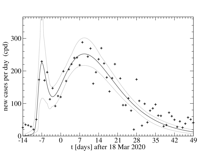
Figure 10: A two-peak fit to the COVID-19 cpd data of Norway, using the form (55) with two independent parameter sets. Estimated 95% CL limits are shown as dotted lines.

The fitted parameters for the early Norwegian peak are ${\rm P}_{max}=764$ [cases], $\tau=1.44$ [days], and $t_{0}=-7.06$ [days]. The very similar early peak in Denmark gave the parameters ${\rm P}_{max}=778$ [cases], $\tau=1.22$ [days], and $t_{0}=-7.21$ [days]. The total cases predicted for Denmark and for Norway are simply the sum of the early and later peaks, thus $11.01k$ and $7.72k$ cases respectively.

IV.6 SHIR model fits to multiple countries

The idea of simultaneously fitting multiple countries to the SHIR model seems appealing, particularly as this model gives a good description of the case numbers from many different European countries. Unfortunately there are complications with this procedure; individual countries vary considerably in the fitted values of the total cases ${\rm P}_{max}$, the characteristic social response time $\tau$, and the local time of the pandemic peak, $t_{0}$. These differences suggest a scaling approach, in which we determine these parameters separately for each country in a SHIR model fit, and then translate (by $t_{0}$) and scale (by ${\rm P}_{max}$ and $\tau$) the datasets for each country separately. If the model and the data are both accurate, these translated and scaled datasets should provide points that fall on the universal curves shown in Figs.5 and 6. Of course there are indications that the COVID-19 data itself is occasionally problematic, with considerable scatter, single-bin spikes, and in some countries a modulation with a 7-day period that may reflect a weekly reporting regimen. Nonetheless it is of interest to generate this translated and scaled scatterplot, to see whether a common pandemic profile is indeed evident in the European data.

This scatterplot is shown in Fig.11 for the 82-point cpd datasets of all 15 European countries in Table.1. Each national dataset was translated and scaled separately by its particular values of $t_{0}$, ${\rm P}_{max}$, and $\tau$ (as given in the table) before being added to this figure. The data from Denmark and Norway before 20 Mar 2020 was excluded from the plot, to suppress contributions from their initial early outbreaks.

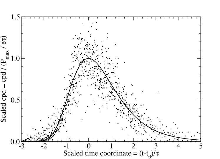
Figure 11: A universal scatterplot of 1162 cpd data points from the 15 European countries of Table.1, translated and scaled to fit on the universal plot for $d{\rm P}/dt$, Fig.6. The (parameter-free) SHIR model prediction for $d{\rm P}/dt$, Eq.(68), is shown as a solid line in this figure.

The scaled, centered universal curve for $d{\rm P}/dt$ is shown as a solid line in Fig.11, and is given by

$$\frac{d{\rm P}}{dt}\Bigg{/}\frac{{\rm P}_{max}}{e\tau}=\frac{e^{-((t-t_{0})/\tau\,-1)}}{\exp(e^{-(t-t_{0})/\tau})}\ .$$ (68)

We can use this scatterplot to combine the data from the 15 European countries we have considered, since they have now been superimposed through translating in time and scaling both axes. On binning in the scaled time variable $(t-t_{0})/\tau$, we can calculate the average and variance of the scaled cpd datapoints in each bin, which provides an average and error for $d{\rm P}/dt$ at that value of $(t-t_{0})/\tau$. As an example, we have used bins of width $\Delta(t-t_{0})/\tau=0.5$, centered on $t-t_{0}=0$, which gives the result shown in Fig.12. This appears approximately consistent with the parameter-free SHIR model result for $d{\rm P}/dt$ (68), although there may be relatively minor discrepancies at onset ($(t-t_{0})/\tau\approx-2$) and well after peak ($(t-t_{0})/\tau\approx 3-4$).

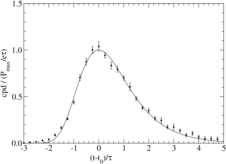
Figure 12: A country-averaged curve for $d{\rm P}/dt$ obtained by binning the 15 datasets in Fig.11 and averaging within each time bin. The resulting $d{\rm P}/dt$ values are shown together with the parameter-free SHIR model prediction (68).

The Europe-averaged COVID-19 data for the new cases per day shown as points with errors in Fig.12 can be used to calculate expectation values under this common COVID-19 $d{\rm P}/dt$ distribution. Some of these results are given in Table.3, where they are compared to theoretical values predicted by the SHIR model $d{\rm P}/dt$, Eq.(68). Evidently the simpler expected values are in reasonably good agreement, notably the displaced value of the mean from the maximum. There is however a discrepancy in the cubic expected values, which are sensitive to the relatively less well determined wings of the distribution at larger $|t-t_{0}|/\tau$.

Quantity	SHIR theory	SHIR num.	COVID data
Area	e	2.7180	002.787 (25)
$x$	$\gamma$	0.5772	000.5746 (28)
$x^{2}$	$\gamma^{2}+\pi^{2}/6$	1.9780	001.996 (52)
$\sigma$	$\pi/\sqrt{6}$	1.2830	001.291 (8)
$x^{3}$	$\gamma^{3}+\gamma\pi^{2}/2+2\,\zeta(3)$	5.4400	004.57 (9)
skewness	$12\sqrt{6}\,\zeta(3)/\pi^{3}$	1.1400	000.70 (19)

Table 3: Expected values of several quantities calculated using the theoretical SHIR model cases per day distribution function $d{\rm P}/dt$ (68), compared to the results found using the Europe-averaged COVID-19 data shown in Fig.12. Here for simplicity we abbreviate $(t-t_{0})/\tau=x$.

IV.7 Future prospects

We have shown that a SHIR (generalized SIR) model and its associated differential equations give rather good closed-form results for the COVID-19 data on new cases per day and cumulative cases, when solved under certain assumptions. These assumptions can be relaxed in future studies.

One important assumption was to ignore the effects of the “resolved” population fraction ${f_{\rm R}}$. This quantity, which is certainly of interest in planning economic recovery, is simple to evaluate from the “infected” fraction we have discussed here; it is simply the integral in Eq.26. This can be evaluated analytically, together with the full DE for ${f_{\rm I}}$, including the $r_{\rm R}$ term, to accommodate transitions out of “infected” and into “resolved.” The cumulative case numbers ${\rm P}(t)$ discussed in relation to COVID-19 data should then be defined by ${\rm P}(t)={\rm N}_{0}(f_{\rm I}+f_{\rm R})$, i.e. “infected” plus “resolved,” since $f_{\rm R}$ is no longer assumed to be negligible.

Calculations of mortality rates are certainly of interest, and are implicitly included in the transition from the infected population ${\rm I}$ (or ${\rm I}_{\rm S}$) to the resolved population ${\rm R}$. Mortality can easily be treated separately, for example by specifying separate ${\rm I}\to{\rm R}$ rate parameters for mortality and for recovery. In the extended SHIR model of Fig.13, mortality would presumably only contribute to the combined rate for ${\rm I}_{\rm S}\to{\rm R}$. The mortality rate coefficients may of course depend strongly on the procedures followed at each country’s medical facilities.

Numerical methods can be used to extract SHIR model results for the full model, including the ${\rm S}-{\rm I}$ quadratic infection term, and can test the importance of the “small fraction of infections” approximation used here.

A straightforward generalization of the model could accommodate the effect of “asymptomatic” infected individuals on the dynamics of the COVID-19 pandemic. Recent antibody results from Italy Lav20 suggest that the asymptomatic cases are a large but not dominant fraction of all COVID-19 cases. Once better data on the number of asymptomatic cases becomes available, it may prove useful to extend the model to include this population. This group follows a progression ${\rm S}\to{\rm I}_{\rm A}\to{\rm R}$, and while in the ${\rm I}_{\rm A}$ population presumably contributes to the infection of other individuals still in ${\rm S}$. Although adding this branch to the model may indicate that the fraction of resolved individuals ${f_{\rm R}}$ is much larger than the SHIR model alone suggests, the pathway through symptomatic cases will remain as before. The most visible predictions of the model, for the number of symptomatic cases (now ${\rm I}_{\rm S}$), may not change significantly. A block diagram of this extended SHIR model is shown in Fig.13.

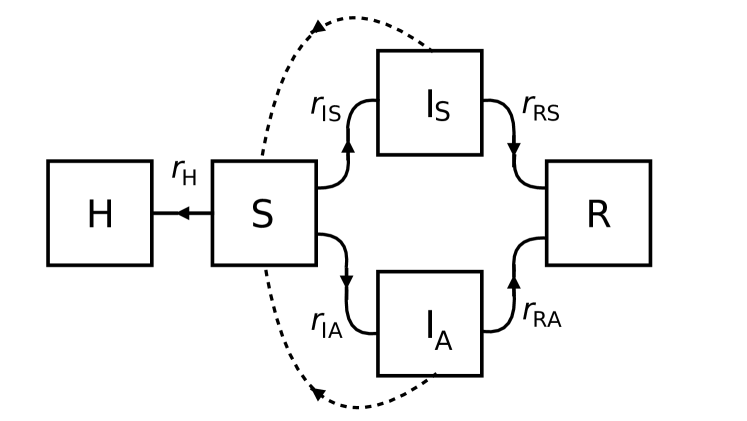
Figure 13: An extended SHIR model block diagram including an asymptomatic line.

Finally, although we have primarily considered COVID-19 in Central and Western European countries, largely because of an assumed similarity in standards for reporting data, there is extensive data available from many other countries which could be addressed using this type of model, undoubtedly with interesting results.

V Summary and Conclusions

In this paper we have introduced a generalization of the SIR model in order to incorporate the effects of pandemic reduction measures. This “SHIR” model adds a rate process that allows transitions from the susceptible population (S) to a new “hidden” population (H), which we assume is not susceptible to infection. We have solved this model analytically in the limit of a small infected population fraction, and showed that the predicted time dependence of cumulative cases and new cases per day is in surprisingly good agreement with COVID-19 data. (We primarily considered Central and Western European countries in this study.) The solution of the model with our approximations involves three free parameters; one is the “social response time” $\tau$, which varies widely between countries, in a manner that correlates with their coronavirus policies.

VI Acknowledgments

We are happy to acknowledge useful communications with and suggestions from P.Ardanuy, D.Arovas, F.E.Close, E.Kioski, S.Nagler, M.Osmann, J.-L.Rosenthal, M.Savage, M.Shinn, D.J.Smith, D.A.Spong and E.S.Swanson during the production of this manuscript. We are also grateful to E.S.Swanson for assistance with calculations of expected values and errors in the SHIR model, and with the model block diagrams.

References

- (1) K. Rock, S. Brand, J. Moir and M.J.Keeling, “Dynamics of infectious diseases” Rep. Prog. Phys. 77, 026602 (2014). http://doi.org/10.1088/0034-4885/77/2/026602
- (2) In this simple SIR model the time at which is a maximum and that maximum value can be solved for analytically, and are respectively and , where .
- (3) W. O. Kermack and A. G. McKendrick, “A contribution to the mathematical theory of epidemics” Proc. R. Soc. Lond. A115, 700 (1927). http://doi.org/10.1098/rspa.1927.0118.
- (4) Protected groups similar to the “H” box of Fig.2 have previously been considered in generalizations of the SIR model. For example, the effects of vaccination are discussed using an SIRV model Roc2014 , and the 2003 SARS model of Lipsitch et al. Lipsitch2003 introduces an XQ population to model quarantine.
- (5) M. Lipsitch et al., “Transmission Dynamics and Control of Severe Acute Respiratory Syndrome.” Science 3000 (5627), 1966-1970; doi: 10:1126/science.1086616.
- (6) The use of “resolved” for the post-infected population , the sum of deceased and recovered, was suggested by P.Ardaury. This population is also referred to as “closed cases” in the Worldometer COVID-19 database WCU .
- (7) “Worldometer Coronavirus Updates” URL: www. worldometers. info / coronavirus / countries .
- (8) B. Gompertz, “On the Nature of the Function Expressive of the Law of Human Mortality, and on a New Mode of Determining the Value of Life Contingencies.” Phil. Trans. Roy. Soc. London 123, 513-585, (1832).
- (9) Eric W. Weisstein, “Gompertz Curve.” From MathWorld – A Wolfram Web Resource. https:// mathworld. wolfram. com / GompertzCurve.html .
- (10) Skewness is a dimensionless property of a distribution, and is defined by , where the averages here are taken using the distribution .
- (11) We note in passing that a single “outlier” point in the Austrian cpd data, 1321 new cases on 26 Mar 2020, lies above the upper cutoff of 1000 cases per day in Fig.7. It was of course included in the fit. Similarly, the Norwegian cpd data includes an outlier of 399 new cases on 27 Mar 2020 and a negative entry of -44 new cases on 08 Apr 2020, which we assume was a correction to the data. These points were included in the Norwegian fit shown in Fig.(10).
- (12) It is notable that the estimated parameter errors in the cumulative “cas” data fit are much smaller than in the preceding new cases per day “cpd” fit. The cas parameter errors are likely underestimated, since the cas data points represent a running sum, and are therefore highly correlated. The cpd parameter errors are presumably more realistic, since they are not correlated in this manner. Note that the differences between the fitted cpd and cas parameters are comparable to the cpd errors.
- (13) M. Paterlini, Nature 580, 574 (2020). doi: 10.1038/ d41586-020-01098-x .
- (14) Prime Minister M. Rutte, National Address (16 Mar 2020), https:// www.rijksoverheid.nl/ documenten/ toespraken/ 2020/03/16/ tv-toespraak-van-minister-president-mark-rutte. English translation, https:// nltimes.nl/ 2020/03/16/ coronavirus-full-text-prime-minister-ruttes-national-address.
- (15) British Prime Minister Boris Johnson Coronavirus Address (23 Mar 2020). https:// www.c-span.org/ video/ ?470622-1/ british-prime-minister-announces-lockdown-televised-address.
- (16) Lavezzo, E. et al., “Suppression of a SARS-CoV-2 outbreak in the Italian municipality of Vo’.” Nature https:// doi.org/10.1038/s41586-020-2488-1 (2020).