A computational study for the inventory routing problem

Abstract

In this work we compare several new computational approaches to an inventory routing problem, in which a single product is shipped from a warehouse to retailers via an uncapacitated vehicle. We survey exact algorithms for the Traveling Salesman Problem (TSP) and its relaxations in the literature for the routing component. For the inventory control component we survey classical mixed integer linear programming and shortest path formulations for inventory models. We present a numerical study comparing combinations of the two empirically in terms of cost and solution time.

1 Introduction

The inventory routing problem (IRP) is a distribution problem combining inventory control and vehicle routing. In an IRP products are shipped from a warehouse to several geographically dispersed retailers by means of vehicles (the routing component). The warehouse and retailers must manage their inventories without causing stock-outs (the inventory control component). IRPs try to answer the following questions:

• When should products be delivered to the retailers?

• What product quantities should be delivered to each visited retailer?

• Which routes should be taken?

• Which time periods should be replenishment periods?

The objective is to minimize the sum of expected inventory and transportation costs during the planning horizon.

The routing component alone makes the IRP a challenging problem. It reduces to the traveling salesman problem (TSP) when the planning horizon is one, the inventory costs are zero, the vehicle capacity is infinite, and all customers need to be served. Even with only one customer some variants remain computationally hard

The IRP has several variations: the planning horizon can be finite or infinite; the number of products can be one or more; inventory holding cost can be taken into account or not, and can be charged at the warehouse, at the retailers or both; trucks, warehouses and retailers may be capacitated or uncapacitated; and demands for each retailer can be deterministic or stochastic, stationary or non-stationary. The IRP variation treated in this paper is as follows: there is a set of retailers with deterministic but time varying demands; a single product; trucks, warehouses and retailers have unlimited capacity; dispatching a truck has a fixed cost; there are transportation costs associated with the route followed by the truck to reach a given retailer. The problem is to determine the optimal replenishment plan for each retailer and vehicle routes for each replenishment period, while minimising total expected cost.

Most IRP research assumes capacitated warehouse, retailers and trucks, but even without capacity constraints the problem is NP-hard because of the TSP component. It is surprising that no study in the literature has investigated the uncapacitated case, which simply integrates a TSP and a Wagner-Whitin inventory model. There are several formulations in the literature for both of these problems, and investigating their possible combinations could yield useful guidance for future IRP research. Our contribution to the literature is as follows:

• We model the uncapacitated IRP routing component as a TSP and the inventory component as a dynamic lot-sizing problem.

• We explore several combinations of TSP formulations and inventory control models from the relevant literatures.

• We present a numerical study comparing these combinations empirically, in terms of cost and solution time.

The rest of paper is organized as follows. Section 2 introduces the relevant literature. Section 3 explains the relevant TSP and inventory control models. Section 4 provides the definition of our IRP. Section 5 presents the numerical study. Finally, Section 6 draws conclusions.

2 Background

The paper of Federgruen and Zipkin (1984) was among the first to investigate the integration of inventory management and vehicle routing problems. They consider a warehouse with several retailers and a scarce resource available for a single period. They use a fleet of vehicles with limited capacity to deliver product. The demand for each retailer is assumed to be a random variable. The objective is to determine vehicle routes and replenishment quantities while minimizing the expected sum of transportation and inventory costs, the latter including holding and shortage costs. They propose a non-linear mixed integer programming model for this problem, and use generalized Benders’ decomposition that decomposes the problem into (i) an inventory allocation problem with holding and shortage costs, and (ii) a routing problem that can be computed as a TSP for each vehicle with transportation costs.

Dror and Ball (1987) investigate reducing the long-term planning of inventory routing problem to a short-term planning. They consider the case of capacitated vehicles, and present a mixed-integer linear programming (MILP) model under deterministic demands.

Campbell et al. (1998) explore how to model the long-term effects of short-term decisions, and propose two short-term planning approaches. They use a heuristic implemented in a rolling horizon framework that determines a distribution strategy, while minimizing average distribution cost over the planning horizon without causing stock-outs at any retailer.

Anily and Federgruen (1990) analyze the case of a single product and an infinite horizon. The product is shipped from warehouse to retailers that have deterministic demands by using a fleet of capacitated trucks. They propose a heuristic method to determine long-term replenishment and routing plans while minimising transportation and inventory costs.

Chandra and Fisher (1994) consider a plant that produces several products delivered by a fleet of capacitated vehicles. They present a computational study which compares two approaches under deterministic demands: one solves the production scheduling and routing problems seperately, while the other combines the two problems into a single model.

Bertazzi et al. (2002) present a policy called the deterministic order-up-to policy for an IRP. The demand of each retailer is deterministic and can vary over time. Each retailer has a minimum and maximum inventory level and must be visited before its inventory reaches its minimum level. When a retailer is visited the inventory level is increased up to the maximum level. They propose a heuristic to determine a shipping policy that minimizes transportation cost and inventory costs both at the supplier and the retailers. Archetti et al. (2007) present a MILP model for this problem and solve the model optimally.

Gaur and Fisher (2004) tackle a real-world problem for Albert Heijn (a supermarket chain in the Netherlands). They assume that a single product with deterministic time-varying demand is delivered via a fleet of capacitated vehicles. They present a solution method for a periodic IRP: first they determine the delivery times and vehicle routes; then trucks are assigned to the routes; finally, workload balancing is used to adjust the departure times.

Bertazzi et al. (2008) analyse how transportation and inventory costs affect the optimal cost, and the impact of vehicle capacity and inventory holding capacity on distribution strategies, under deterministic demands.

As can be seen from this survey, no previous studies have explored the usefulness of TSP/Wagner-Whitin formulation combinations.

3 Formulations of TSP and Inventory Control Models

This section surveys known MILP formulations for the two components of the IRP.

3.1 Formulations of TSP

A large number of TSP formulations have been presented in the literature, and we survey several MILP formulations.

The objective is to find the shortest route that starts from an initial city, visits every city exactly once and returns back to the initial city. The integer linear program (ILP) formulation of Dantzig et al. (1954) was one of the first. $R=\{1,2,\ldots,r\}$ is the set of cities which are visited and $c_{ij}$ the distance between each pair of cities. $x_{ij}$ is a binary decision variable which takes the value 1 if and only if the salesman travels from city $i$ to city $j$. The formulation of Dantzig et al. (1954) is as follows:

$$\text{Minimize}\quad\quad\sum_{i=1}^{r}\sum_{j=1}^{r}(x_{ij}c_{ij})\hfill$$ (1)

$$\text{Subject to}\quad\sum_{i=1i\neq j}^{r}x_{ij}=1\quad\forall j\in R\hfill$$ (2)

$$\quad\sum_{j=1i\neq j}^{r}x_{ij}=1\quad\forall i\in R\hfill$$ (3)

$$\sum_{i,j\in S}x_{ij}\leq|S|-1\quad\forall S\subseteq R,\quad 2\leq S\leq r-2\hfill$$ (4)

$$x_{ij}\in\{0,1\}\hfill$$ (5)

Eq. (2) and Eq. (3) are called assignment constraints. Eq. (2) ensures that the salesman must leave each city once while Eq. (3) ensures that the salesman must enter each city once. Eq. (4) are called subtour elimination constraints, and prevent the formation of subtours (tours involving proper subsets of the cities).

Miller et al. (1960) proposed a MILP formulation by introducing a new continuous variable $u_{i}$ to reduce the number of subtour elimination constraints. $u_{i}$ denotes sequence number in which retailer $i$ is visited. While the objective function Eq. (1) and assignment constraints Eq. (2) and Eq. (3) remain the same, the subtour eliminiation costraints are as follows:

$$u_{i}-u_{j}+rx_{ij}\leq r-1\quad\forall i,j=2,3,\ldots,r\quad i\neq j$$ (6)

Desrochers and Laporte (1991) proposed an alternative subtour elimination constraints with a stronger relation between $u_{i}$ and $x_{ij}$ improving the constraints of Miller et al. (1960).

$$u_{i}-u_{j}+(r-1)x_{ij}-(r-3)x_{ji}\leq r-2\\ \quad\forall i,j=2,3,\ldots,r\quad i\neq j$$ (7)

Gavish and Graves (1978) presented a flow-based formulation which can be used for some transportation problems as well as the TSP. They introduced new continuous variables $y_{ij}$ to represent the flow between cities $i$ and $j$ to reformulate the subtour elimination constraints. In their formulation, called the single commodity flow formulation by Orman and Williams (2006), objective function Eq. (1) and assignment constraints Eq. (2) and Eq. (3) are retained while subtour elimination constraints as follows:

$$y_{ij}\leq(r-1)x_{ij}\quad\forall i\in R\quad\forall j\in R\quad i\neq j$$ (8)

$$\sum_{j\neq 1}^{r}y_{1j}=r-1$$ (9)

$$\sum_{j=1i\neq j}^{r}y_{ij}-\sum_{j=2i\neq j}^{r}y_{ji}=1\quad i=2,3,\ldots,r$$ (10)

$$y_{ij}\geq 0$$ (11)

Finke et al. (1984) proposed an integer formulation taking the form of two commodity network flow problems. They introduced continuous variables $y_{ij}$ to represent the flow of commodity 1 between cities $i$ and $j$, and$z_{ij}$ to represent the flow of commodity 2 between cities $i$ and $j$. They retain the objective Eq. (1) and assignment constraints Eq. (2) and Eq. (3), while the subtour elimination constraints are:

$$\sum_{j=2}^{r}(y_{1j}-y_{j1})=(r-1)$$ (12)

$$\sum_{j=2}^{r}(z_{1j}-z_{j1})=-(r-1)$$ (13)

$$\sum_{j=1}^{r}(y_{ij}-y_{ji})=-1\quad i=2,\ldots,r\quad\forall i\neq j$$ (14)

$$\sum_{j=1}^{r}(z_{ij}-z_{ji})=1\quad i=2,\ldots,r\quad\forall\neq j$$ (15)

$$\sum_{j=1}^{r}(y_{ij}+z_{ji})=r-1\quad i=1,\ldots,r\quad\forall i\neq j$$ (16)

$$(y_{ij}+z_{ij})=(r-1)x_{ij}\quad i,j=1,\ldots,r\quad\forall i\neq j$$ (17)

$$y_{ij},z_{ij}\geq 0$$ (18)

Bektaş and Gouveia (2014) proposed a systematic way to find a generalization of the inequalities of Miller et al. (1960) (referred to as MTZ) and Desrochers and Laporte (1991) (referred to as DL), via a polyhedral approach that studies and analyzes the convex hull of feasible sets. Because MTZ has a weak linear programming (LP) relaxation, they proposed new inequalities with a strong LP relaxation. First they implemented this approach for two sets and reinvented the MTZ and DL inequalities. Then they obtained a generalization of these inequalities which implies the constraints proposed by Dantzig et al. (1954), referred to as CLIQUE for three-node subsets. A weaker version of constraints Dantzig et al. (1954) are the CIRCUIT inequalities which are given as follows:

$$\sum x_{ij}\leq|C|-1\quad\forall C\in G_{v_{1}}$$ (19)

where $G_{v_{1}}$ is the complete graph induced by the set of nodes $v_{1}=2,\ldots,r$ and $C$ is any set of arcs defining an elementary circuit in $G_{v_{1}}$.

They illustrate a two-node version of the CLIQUE constraints (2CLQ) as follows:

$$x_{ij}+x_{ji}\leq 1\quad i,j=2,\ldots,r$$ (20)

The DL inequalities generalized to three nodes are:

$$u_{i}-u_{k}+(r-1)(x_{ij}+x_{jk})+(r-3)(x_{kj}+x_{ji})\\ +rx_{ik}+(r-4)x_{ki}\leq 2r-4$$ (21)

$$2u_{i}-u_{j}-u_{k}+(2r-2)(x_{ij}+x_{ik})+(2r-8)(x_{ji}+x_{ki})+\\ (2r-5)(x_{jk}+x_{kj})\leq 4r-10$$ (22)

$$-2u_{i}+u_{j}+u_{k}+(2r-8)(x_{ij}+x_{ik})+(2r-2)(x_{ji}+x_{ki})+\\ (2r-5)(x_{jk}+x_{kj})\leq 4r-10$$ (23)

The CLIQUE constraints can be obtained for three nodes (3CLQ) by adding Eq. (22) for triple $(i,j,k)$ to Eq. (23) for the same triple. The new constraints Eq. (21) and Eq. (22) for triples $(i,j,k)$, $(k,i,j)$ and $(j,k,i)$ are respectively called non-radical (NR) and radical (R) constraints. A different class of inequalities called 2PATH constraints are also presented in Bektaş and Gouveia (2014):

$$u_{i}-u_{k}+(2r-3)x_{ik}+(r-4)x_{ki}+\\ (r-1)(x_{ij}+x_{jk})\leq 2r-4\quad i\neq j\neq k$$ (24)

$$u_{k}-u_{i}+(2r-7)x_{ik}+(r-1)x_{ki}+\\ (r-4)(x_{ij}+x_{jk})\leq 2r-6\quad i\neq j\neq k$$ (25)

These constraints imply a lifted version of the CIRCUIT inequalities Eq. (19), and the summation of constraints Eq. (24) and Eq. (25) for $(i,j,k)$ gives the lifted circuit inequalities (L3).

3.2 Inventory Control Models

Inventory control has an important role in terms of matching supply and demand effectively. Its aim is to determine the time and quantity of replenishment orders while minimizing inventory costs. In this section we focus on two deterministic inventory models for the well-known Wagner and Whitin (1958) problem.

We first give a MILP formulation for the Wagner and Whitin (1958) problem. Consider an $N$-period planning horizon indexed by $t\in\{1,2,\ldots,N\}$. Assume that demand $d_{t}$ in period $t$ is deterministic. A fixed holding cost $h$ is incurred if any item is carried from one period to the next. A unit cost $v$ is incurred for each item ordered. A fixed ordering cost $K$ is incurred each time an order is placed. The decision variables in this problem are as follows: $q_{t}$ represents the quantity ordered at period $t$. $I_{t}$ represents inventory level at period $t$. $\delta_{t}$ is a binary decision variable that takes value 1 if and only if an order is placed at period $t$. The formulation is:

$$\text{Minimize}\quad\quad\sum_{t=1}^{n}(K\delta_{t}+hI_{t}+vq_{t})$$ (26)

$$\text{Subject to}\quad\quad I_{t}=\begin{cases}I_{0}+q_{t}-d_{t},&\text{if $t=1$}.\\ I_{t-1}+q_{t}-d_{t},&\text{otherwise}.\end{cases}\\ \quad t=1,2,\ldots,n\\$$ (27)

$$q_{t}\leq\sum_{k=t}^{n}d_{k}\delta_{k}\quad\textrm{for}\quad t=1,2,\ldots,n$$ (28)

$$I_{t},q_{t}\geq 0,\quad t=1,2,\ldots,n$$ (29)

The dynamic programming formulation proposed by Wagner and Whitin (1958) can also be formulated as shortest path network flow. The objective of the shortest path problem is to determine the shortest route between source and destination. The network is a directed acyclic graph with several nodes between source and destination. It consists of $N+1$ nodes representing periods to take into account the cost of the last period. The first period represented by node 1 is the source and the destination is node $N+1$. Arc $(i,j)$ is traversed if an order is placed at period $i$ to cover demands from period $i$ to period $j-1$, and at period $j$ the next order is placed. So $\omega(i,j)$ can refer to the inventory cost including ordering costs and holding cost incurred from period $i$ to period $j-1$ (see Muckstadt and Sapra (2010)).

$$\omega(i,j)=K+\sum_{k=i}^{j}vd_{k}+h\sum_{k=i}^{j}(k-i)d_{k}\quad i,j=1,\ldots,n+1\quad i<j$$ (30)

The decision variable $w_{ij}$ determines whether an order is placed at period $i$ to satisfy demand of period $i,i+1,\ldots,j-1$. Hence the shortest path LP formulation for the inventory control problems is given as follows:

Minimize

$$\sum_{i,j\in N}\omega(i,j)w_{ij}$$ (31)

Subject to

$$\sum_{j\in N+1}w_{ij}-\sum_{j\in N+1}w_{ji}=\begin{cases}1&\text{if $i=1$}\\ -1&\text{if $i=n+1$}\\ 0&\text{Otherwise}\\ \end{cases}\quad\quad i,j=1,\ldots,n+1\\$$ (32)

$$w_{ij}\geq 0$$ (33)

4 Definition of the Inventory Routing Problem

We consider a system which a single product is shipped from a warehouse (W) to a set of retailers $R=\{1,2,\ldots,r\}$ over a finite planning horizon $N$. We assume that for each period $t\in\{1,2,\ldots,N\}$ the demand $d_{ti}$ of any retailer $i\in\{1,2,\ldots,R\}$ is known. A truck departs from the warehouse, visits all the retailers which are replenished once, then returns back to the warehouse via the route with minimum distance. The truck does not necessarily visit all retailers at each period. It is assumed that the capacities of the warehouse, truck, and retailers are unlimited.

The parameters of the problem are defined as follows. A holding cost $h_{i}$ is incurred if any item is carried from one period to the next by any retailer (we ignore unit ordering cost $v$ in this problem). A fixed ordering cost $K$ is incurred each time an order is placed by any retailer. The distance $c_{ij}$ between retailers $i$ and $j$ is known. The decision variables of the problem are as follows: $x_{tij}$ is a binary decision variable from the TSP component that determines whether the truck travels from city $i$ to $j$ in period $t$. From the inventory component, $q_{ti}$ represents the quantity ordered at retailer $i$ in period $t$, and $I_{ti}$ represents the inventory level of retailer $i$ at the end of period $t$. Retailers have zero initial and final inventory levels. Also from the inventory component, $\delta_{ti}$ is a binary decision variable which takes the value 1 if an order is placed by retailer $i$ in period $t$, and $w_{itk}$ determines whether an order is placed at period $t$ to satisfy demand at period $t,t+1,\ldots,k-1$ for retailer $i$ in the shortest path formulation.

We aim to find the optimal replenishment plan and vehicle routes that minimize the total cost, including inventory cost and transportation cost, without stock-outs at any retailers. We use TSP formulations to determine routing for each replenishment period and inventory control models to determine replenishment quantity for each retailer mentioned in Section 3. We combine the MTZ, DL and TSP models proposed by Bektaş and Gouveia (2014) with the Wagner and Whitin’s MILP inventory model by using assignment constraints (Eq. (2) and Eq. (3)).

$$\sum_{i=1i\neq j}^{r+1}x_{ij}=\delta_{tj}\quad\forall j\in R\cup\{W\}\hfill$$ (34)

$$\quad\sum_{j=1i\neq j}^{r+1}x_{ij}=\delta_{ti}\quad\forall i\in R\cup\{W\}\hfill$$ (35)

Eq. (34) and Eq. (35) ensure that if there is an order at a retailer then the truck must visit that retailer. For the combination of single commodity (SC) flow formulation and Wagner and Whitin’s MILP, we use the following equations in addition to assignment constraints:

$$\sum_{j=1i\neq j}^{r+1}y_{ij}-\sum_{j=2i\neq j}^{r+1}y_{ji}=\delta_{ti}\quad i=2,3,\ldots,r+1$$ (36)

$$\sum_{j\neq 1}^{r}y_{1j}=(r-1)\delta_{tj}$$ (37)

For the combination of the two commodity (2C) flow formulation and Wagner and Whitin’s MILP, the assignment constraints remain the same while the linking constraints are:

$$\sum_{j=2}^{r+1}(y_{1j}-y_{j1})=(r-1)\delta_{ti}$$ (38)

$$\sum_{j=2}^{r+1}(z_{1j}-z_{j1})=-(r-1)\delta_{ti}$$ (39)

$$\sum_{j=1}^{r+1}(y_{ij}-y_{ji})=-1\delta_{ti}\quad i=2,\ldots,r+1\quad\forall i\neq j$$ (40)

$$\sum_{j=1}^{r+1}(z_{ij}-z_{ji})=1\delta_{ti}\quad i=2,\ldots,r+1\quad\forall\neq j$$ (41)

$$\sum_{j=1}^{r+1}(y_{ij}+z_{ji})=(r-1)\delta_{ti}\quad i=1,\ldots,r+1\quad\forall i\neq j$$ (42)

For models relying on the shortest path network flow formulation of Wagner and Whitin (1958) model the linking constraints are redefined by using decision variables $w_{itk}$.

5 Numerical Study

In this section we conduct two types of numerical study to compare the solution times of optimal algorithms, and evaluate the strengths of linear relaxation models.

First we consider the instance set proposed by Archetti et al. (2007). There are two types of planning horizon lengths $N\in\{3,6\}$. We have one warehouse and ten possible values of retailers such that $r=5k$ ($k=1,2,\ldots,10$) when the planning horizon is $3$. If the planning horizon is $6$ then we have six possible values of retailers such that $r=5k$ ($k=1,2,\ldots,6$). We assume that the warehouse has sufficient product for its retailers, and that there is no initial inventory at any retailer. The demand for each retailer is deterministic and constant for each period. The demand is a uniformly distributed random integer in the interval $[10,100]$. There are different holding costs for each retailer, uniformly randomly distributed in the interval $[0.01,0.05]$. There is no holding cost for the warehouse. We consider inventory costs at retailers and transportation costs between warehouse and retailers. The fixed ordering cost is $10$. The distance $c_{ij}$ between retailers $i$ and $j$ is given by Euclidean geometry: $c_{ij}=\sqrt{(x_{i}-x_{j})^{2}+(y_{i}-y_{j})^{2}}$ where coordinates $(x_{i},y_{i})$ and $(x_{j},y_{j})$ are uniformly distributed random integers in the interval $[0,500]$. In this numerical design the complexity of TSP dominates that of the inventory component, and the computational times depend mainly on the configuration of retailers (Tables I—R).

In our second numerical design, based on instances derived from the academic literature on the TSP and inventory management, we focus instead on problems in which inventory control occurs over a longer planning horizon of 15. We have one warehouse and one type of retailer set of 16 retailers (TSPLIB ). A truck with unlimited capacity delivers products. We assume that the demand of any retailer is deterministic for each period, but with three demand patterns. In the first demand pattern each retailer has the same stationary demand (STA) of 100 in each period. In the second demand pattern retailers have different stationary demand patterns: the demand for five retailers is 100 for each period, the demand for six other retailers is 50 and for the rest 75 for each period. The last demand pattern is a combination of stationary demand pattern, two life cycle patterns (LCY1 and LCY2), two sinusoidal patterns (SIN1 and SIN2) and a random pattern (RAND). We adopt demand patterns from Rossi et al. (2015). Figure A illustrates these demand patterns. We consider three types of fixed ordering cost $K$: first, no fixed ordering cost; secondly, a fixed ordering cost of 1000 for each retailer; finally, a fixed ordering cost of 500 for five retailers, 1000 for six other retailers and 2000 for the remaining five retailers. In this numerical design we also have dispatching cost $D$ which is incurred if the truck visits any nonzero number of retailers. We have two types of dispatching cost $D\in\{0,15000\}$. We assume that the warehouse has sufficient product to deliver to retailers, and that there is no initial inventory at any retailer. There is no holding cost for the warehouse, and the holding cost is 1 for each retailer. For each combination of $K$, $D$ and demand patterns we generate 18 scenarios.

The results are presented in Tables B–H which show the computational times (in seconds) and optimality gap (%) of different combinations. We set a time limit of 1 hour and record the optimality gap if a problem is not solved optimally. CMILP and SP respectively denote classical MILP and shortest path formulations for inventory control. MTZ, MTZ+2Clq, DL, SC and 2C denote the exact TSP algorithms mentioned in Section 3. In Scenarios 1–3 we assume that there is no fixed ordering cost and dispatching cost. Retailers have three types of demand pattern; same STA demand, different STA demand and combination of STA, LCY1, LCY2, SIN1, SIN2 and RAND. In Scenarios 4–6 there is a fixed ordering cost of 1000 and no dispatching cost. Three demand patterns are used. In Scenarios 7–9 we have the same demand patterns and retailers have different fixed ordering costs: 500 for five retailers, 1000 for six others and 2000 for the remaining five retailers. There is no dispatching cost. In Scenarios 10–18 we assume that the dispatching cost is 15000 and we use the same combinations as in Scenarios 1–9.

Table B and Table B show the same information. Table B shows that the CMILP+MTZ, CMILP+MTZ+2CLQ and CMILP+DL combinations do not yield optimal solutions within the time limit. However, the results of Scenarios 4–9 (in the presence of fixed ordering cost only) are very close to optimal. CMILP+SC yields optimal solutions for all scenarios except 1. CMILP+2C is very close to optimal in most scenarios. Table B provides similar results but its computational times are longer.

Tables C and D show the optimality gaps for the LP relaxations of the combination of inventory models and TSP algorithms. As expected, the LP relaxation of CMILP+MTZ is furthest from optimal. The LP relaxations of CMILP+MTZ+2CLQ and CMILP+DL combinations have the same optimality gap. As indicated in Bektaş and Gouveia (2014) the LP relaxation of CMILP+MTZ+2CLQ provides a better approximation than that of CMILP+MTZ. The LP relaxations of CMILP+SC and CMILP+2C combinations yield the same optimality gap. Although the LP relaxations of CMILP+SC and CMILP+2C are slightly worse than those of CMILP+MTZ+2CLQ and CMILP+DL for Scenarios 1–9, the LP relaxations of CMILP+SC and CMILP+2C are best for Scenarios 10–18. Regarding computation times, the LP relaxations of CMILP+MTZ+2CLQ and CMILP+DL are faster than those of CMILP+SC and CMILP+2C for Scenarios 1–12. We also observe that the computation times for the LP relaxation of CMILP+MTZ are greater with the third demand pattern and fixed ordering cost (Scenarios 6, 9, 15 and 18). If we analyse the LP relaxations, SP+SC and SP+2C LP relaxations yield the best approximations for all scenarios, while SP+MTZ gives the biggest optimality gap. The computation times are similar for all combinations and scenarios.

Tables E and G show the optimality gaps for the LP relaxations of the inventory models and TSP formulations proposed by Bektaş and Gouveia (2014). Tables F and H show computation times for these combinations. From Table E and Table G we see that most combinations yield the same optimality gap. While the LP relaxation of CMILP+TSP formulations proposed by Bektaş and Gouveia (2014) provide better approximations than the LP relaxation of CMILP+MTZ, CMILP+MTZ+2CLQ and CMILP+DL, the computational times for the LP relaxations of the CMILP+TSP formulations proposed by Bektaş and Gouveia (2014) are very high. The LP relaxation of the SP+TSP formulations proposed by Bektaş and Gouveia (2014) give slightly better approximations than those of SP+MTZ, SP+MTZ+2CLQ and SP+DL. Comparing the combinations of CMILP and SP with TSP formulations proposed by Bektaş and Gouveia (2014), the CMILP combinations give better approximations but greater computational times.

6 Conclusion

In this paper, we presented combinations of optimal and near-optimal TSP algorithms and inventory models from the literature, to solve an inventory routing problem under deterministic demand over a finite planning horizon.

We tested these algorithms empirically on two types of scenario and found the following results:

• For the combination of exact TSP algorithms and inventory models, CMILP+TSP combinations are faster than SP+TSP combinations and the fastest algorithm is CMILP+SC.

• CMILP+SC and SP+SC combinations are more sensitive as fixed ordering and dispatching cost increase.

• The combinations of TSP formulations proposed by Bektaş and Gouveia (2014) with inventory models provide better approximations than MTZ formulations.

Appendix

In this appendix we illustrate demand patterns used in our computational study and the results of our experiments.

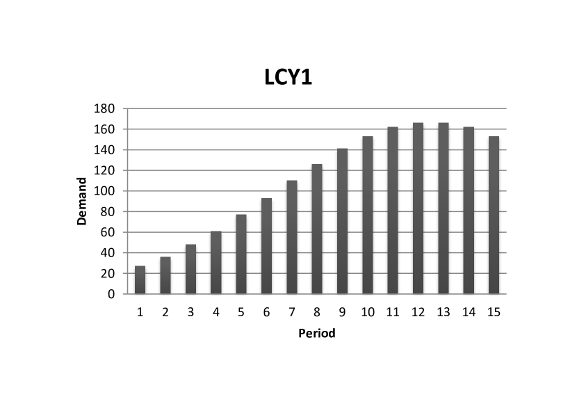
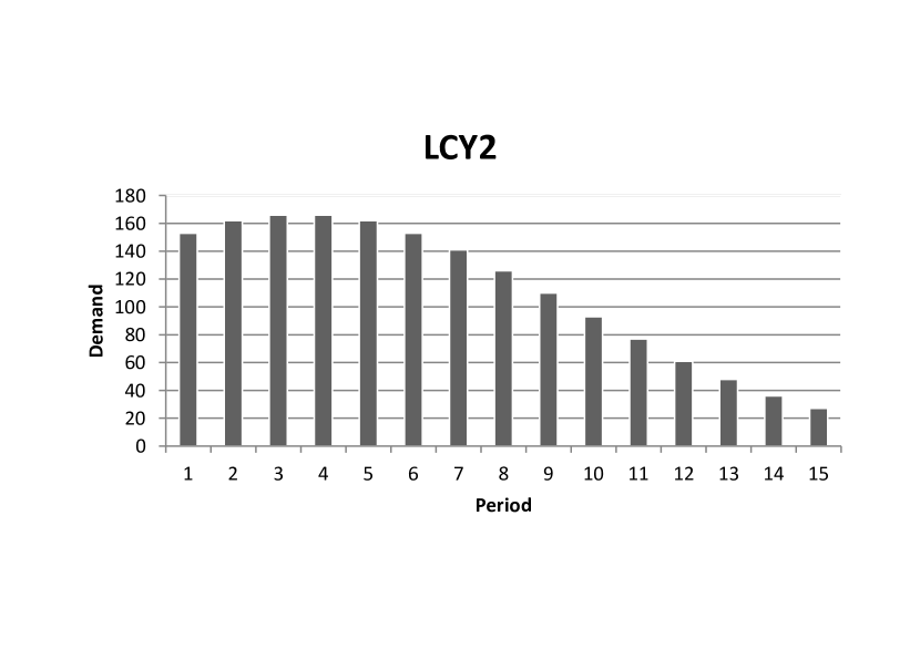
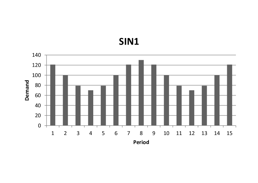
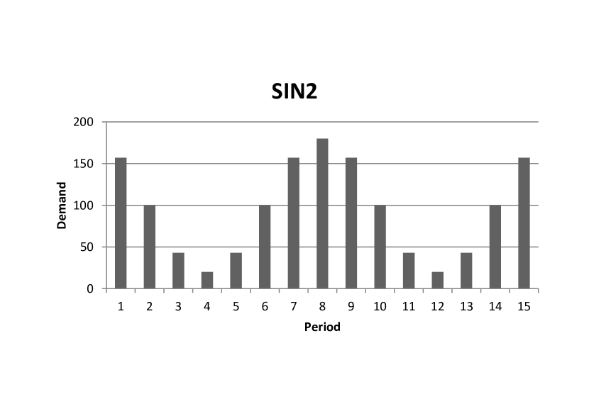
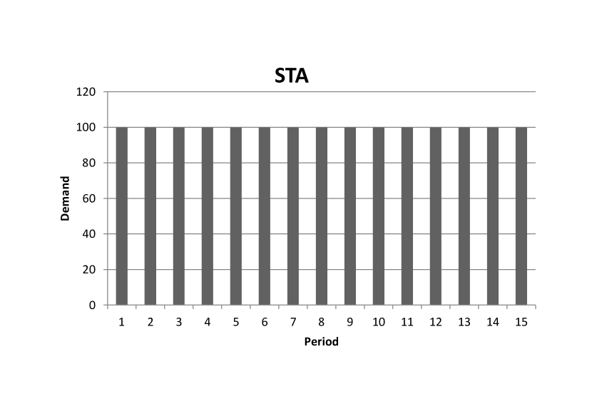
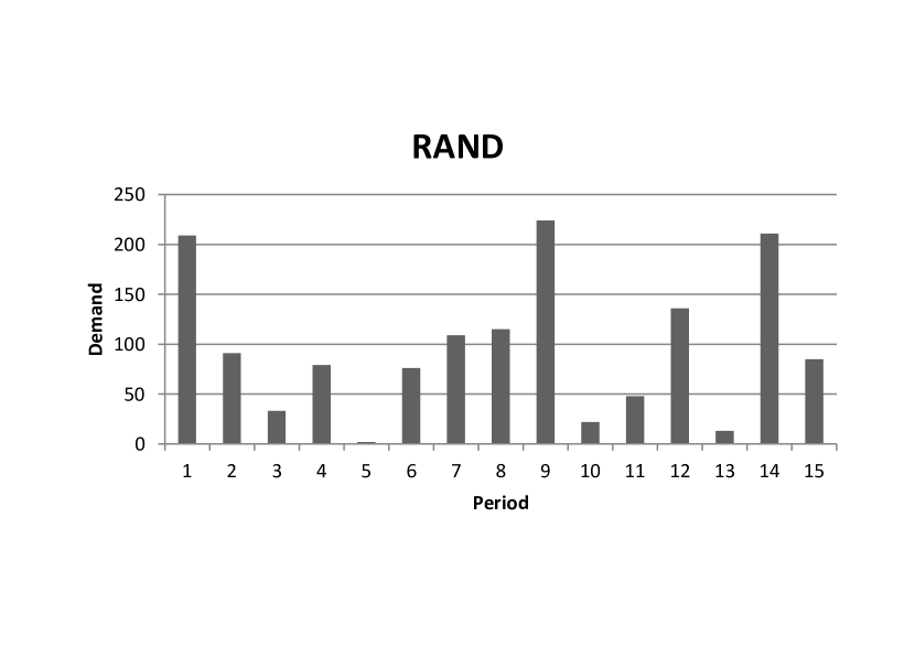
Figure A: Demand Patterns

Table A: The combinations of CMILP and exact algorithms of TSP

	CMILP+MTZ			CMILP+MTZ+2Clq			CMILP+DL			CMILP+SC			CMILP+2C
	Time (sec)	%Gap	Best solution	Time (sec)	%Gap	Best solution	Time (sec)	%Gap	Best solution	Time (sec)	%Gap	Best solution	Time (sec)	%Gap	Best solution
Scenario 1	3600.00	42.60	31000	3600.00	40.16	29740	3600.00	40.63	30360	3600.00	0.33	28740	3600.00	13.85	29120
Scenario 2	3600.00	41.83	28435	3600.00	38.38	27035	3600.00	46.15	30115	190.13	0.00	26265	3600.00	13.12	26435
Scenario 3	3600.00	42.55	30491	3600.00	39.64	29331	3600.00	38.85	29120	241.54	0.00	28027	3600.00	11.54	28145
Scenario 4	3600.00	1.26	103020	3600.00	1.69	103020	3600.00	1.37	103020	132.01	0.00	103020	3600.00	0.74	103020
Scenario 5	3600.00	2.30	90220	3600.00	2.70	90785	3600.00	1.87	90220	149.13	0.00	90220	3600.00	0.95	90220
Scenario 6	3600.00	1.95	102119	3600.00	1.94	102119	3600.00	1.86	102119	186.08	0.00	102119	3600.00	1.10	102328
Scenario 7	3600.00	4.16	111780	3600.00	3.06	110860	3600.00	3.52	111420	245.04	0.00	110520	3600.00	1.81	111140
Scenario 8	3600.00	2.46	94775	3600.00	2.86	94975	3600.00	2.67	94975	199.46	0.00	94775	3600.00	1.04	94775
Scenario 9	3600.00	3.05	108239	3600.00	2.92	108132	3600.00	2.85	108019	218.36	0.00	107893	3600.00	1.72	107989
Scenario 10	3600.00	81.92	101860	3600.00	81.33	101620	3600.00	83.36	113080	168.49	0.00	100020	3600.00	0.65	100020
Scenario 11	3600.00	81.91	92390	3600.00	82.62	98025	3600.00	80.89	88625	154.35	0.00	87270	3600.00	0.46	87270
Scenario 12	3600.00	83.18	110143	3600.00	82.09	104604	3600.00	84.7	118467	423.20	0.00	99808	3600.00	1.21	99808
Scenario 13	3600.00	31.23	148020	3600.00	31.48	148020	3600.00	31.19	148020	134.97	0.00	145080	3600.00	0.16	145080
Scenario 14	3600.00	32.82	131305	3600.00	30.37	126605	3600.00	32.94	131305	87.31	0.00	124255	3600.00	0.10	124255
Scenario 15	3600.00	31.61	145898	3600.00	34.72	153045	3600.00	30.89	144459	199.41	0.00	144279	3600.00	0.10	144279
Scenario 16	3600.00	31.47	157180	3600.00	32.94	160440	3600.00	28.28	150080	140.67	0.00	150080	3600.00	0.25	150080
Scenario 17	3600.00	36.18	143355	3600.00	36.04	143355	3600.00	36.08	143355	116.10	0.00	129255	1970.35	0.00	129255
Scenario 18	3600.00	31.30	152744	3600.00	31.44	152804	3600.00	30.43	150838	161.46	0.00	149279	3600.00	0.15	149279

Table B: The combinations of SP and exact exact algorithms of TSP

	SP+MTZ			SP+MTZ+2Clq			SP+DL			SP+SC			SP+2C
	Time (sec)	%Gap	Best solution	Time (sec)	%Gap	Best solution	Time (sec)	%Gap	Best solution	Time (sec)	%Gap	Best solution	Time (sec)	%Gap	Best solution
Scenario 1	3600.00	55.15	34400.00	3600.00	48.54	30140.00	3600.00	44.69	30380.00	3600.00	30.83	30220.00	3600.00	26.77	30040.00
Scenario 2	3600.00	46.64	28270.00	3600.00	44.82	27755.00	3600.00	47.27	29700.00	3600.00	27.59	26940.00	3600.00	28.86	28055.00
Scenario 3	3600.00	54.20	31808.00	3600.00	47.48	30349.00	3600.00	44.25	29789.00	3600.00	26.69	29187.00	3600.00	30.03	29130.00
Scenario 4	3600.00	1.87	103020.00	3600.00	1.86	103020.00	3600.00	1.69	103020.00	3600.00	0.48	103020.00	3600.00	0.94	103020.00
Scenario 5	3600.00	2.23	90220.00	3600.00	2.44	90220.00	3600.00	2.55	90220.00	3600.00	0.47	90220.00	3600.00	1.00	90220.00
Scenario 6	3600.00	2.51	102179.00	3600.00	2.55	102119.00	3600.00	2.42	102119.00	3600.00	0.75	102119.00	3600.00	1.72	102119.00
Scenario 7	3600.00	3.40	110860.00	3600.00	3.14	110760.00	3600.00	3.17	110980.00	3600.00	0.90	110520.00	3600.00	2.05	110860.00
Scenario 8	3600.00	2.53	94775.00	3600.00	2.41	94775.00	3600.00	2.83	94775.00	3600.00	0.49	94775.00	3600.00	1.60	94775.00
Scenario 9	3600.00	3.41	107989.00	3600.00	4.03	108385.00	3600.00	4.28	108955.00	3600.00	1.28	107893.00	3600.00	1.67	107893.00
Scenario 10	3600.00	86.91	127700.00	3600.00	88.04	136980.00	3600.00	87.48	141600.00	3600.00	0.59	100020.00	3600.00	0.76	100020.00
Scenario 11	3600.00	83.01	93515.00	3600.00	84.36	101725.00	3600.00	83.70	99195.00	3600.00	0.29	87270.00	3600.00	1.13	87270.00
Scenario 12	3600.00	85.87	117240.00	3600.00	88.22	136899.00	3600.00	85.51	119571.00	3600.00	1.83	99808.00	3600.00	0.64	99808.00
Scenario 13	3600.00	31.20	146520.00	3600.00	34.63	154680.00	3600.00	31.97	148200.00	2875.52	0.00	145080.00	3600.00	0.28	145080.00
Scenario 14	3600.00	33.11	131365.00	3600.00	33.02	131485.00	3600.00	30.78	127085.00	111.88	0.00	124255.00	3600.00	0.31	124255.00
Scenario 15	3600.00	35.50	153853.00	3600.00	32.75	147938.00	3600.00	32.22	146438.00	1615.71	0.00	144279.00	3600.00	0.04	144279.00
Scenario 16	3600.00	29.52	152600.00	3600.00	31.87	157900.00	3600.00	31.55	156740.00	879.27	0.00	150080.00	3600.00	0.40	150080.00
Scenario 17	3600.00	29.36	130035.00	3600.00	29.47	130155.00	3600.00	29.24	129735.00	1635.82	0.00	129255.00	3600.00	0.00	129255.00
Scenario 18	3600.00	30.82	151138.00	3600.00	31.42	152398.00	3600.00	30.90	151378.00	3600.00	0.04	149279.00	3438.31	0.00	149279.00

Table C: LP relaxation of CMILP+TSP combinations

	CMILP+MTZ		CMILP+MTZ+2Clq		CMILP+DL		CMILP+SC		CMILP+2C
	Time (sec)	%Gap	Time (sec)	%Gap	Time (sec)	%Gap	Time (sec)	%Gap	Time (sec)	%Gap
Scenario 1	28.50	0.93	32.82	0.62	30.47	0.62	29.80	0.62	31.98	0.62
Scenario 2	28.78	0.93	29.39	0.59	28.38	0.59	30.45	0.59	33.20	0.59
Scenario 3	27.98	0.93	30.29	0.61	29.26	0.61	30.61	0.64	34.00	0.64
Scenario 4	34.07	0.06	42.37	0.04	40.41	0.04	54.90	0.05	74.40	0.05
Scenario 5	46.83	0.07	47.45	0.04	51.04	0.04	93.50	0.05	66.15	0.05
Scenario 6	72.37	0.08	49.84	0.04	82.76	0.04	222.77	0.06	110.68	0.06
Scenario 7	60.86	0.07	49.15	0.04	54.49	0.04	282.69	0.05	151.99	0.05
Scenario 8	52.07	0.08	49.23	0.05	50.50	0.05	119.69	0.06	67.32	0.06
Scenario 9	87.54	0.08	59.45	0.05	70.93	0.05	251.33	0.06	214.50	0.06
Scenario 10	28.95	0.95	31.53	0.87	29.13	0.87	34.17	0.05	45.02	0.05
Scenario 11	28.95	0.95	31.14	0.85	30.48	0.85	32.46	0.06	36.59	0.06
Scenario 12	29.21	0.95	31.08	0.87	30.93	0.87	37.73	0.05	35.18	0.05
Scenario 13	34.69	0.33	53.46	0.31	62.54	0.31	37.50	0.02	39.96	0.02
Scenario 14	42.15	0.32	41.15	0.30	50.80	0.30	32.85	0.03	33.30	0.03
Scenario 15	69.61	0.34	43.10	0.32	78.40	0.32	36.80	0.02	36.36	0.02
Scenario 16	96.88	0.31	49.32	0.29	54.45	0.29	42.30	0.02	35.11	0.02
Scenario 17	53.57	0.32	45.97	0.30	58.71	0.30	37.59	0.02	33.40	0.02
Scenario 18	119.05	0.33	48.88	0.31	56.04	0.31	41.63	0.02	35.51	0.02

Table D: LP relaxation of SP+TSP combinations

	SP+MTZ		SP+MTZ+2Clq		SP+DL		SP+SC		SP+2C
	Time (sec)	%Gap	Time (sec)	%Gap	Time (sec)	%Gap	Time (sec)	%Gap	Time (sec)	%Gap
Scenario 1	39.94	0.98	42.80	0.86	39.89	0.86	40.18	0.62	43.87	0.62
Scenario 2	41.27	0.98	42.13	0.86	41.08	0.86	39.39	0.59	44.37	0.59
Scenario 3	39.93	0.98	42.03	0.85	41.21	0.85	40.13	0.64	45.10	0.64
Scenario 4	40.82	0.07	44.06	0.06	42.62	0.06	43.38	0.05	47.01	0.05
Scenario 5	42.93	0.08	46.39	0.06	42.35	0.06	40.55	0.06	46.65	0.06
Scenario 6	42.53	0.09	45.83	0.08	43.40	0.08	41.31	0.07	47.30	0.07
Scenario 7	42.49	0.08	48.25	0.07	43.40	0.07	43.86	0.06	46.53	0.06
Scenario 8	42.37	0.09	43.55	0.08	43.47	0.08	39.99	0.07	46.58	0.07
Scenario 9	42.62	0.09	43.86	0.08	43.50	0.08	39.02	0.07	46.64	0.07
Scenario 10	41.95	0.96	40.60	0.93	43.49	0.93	39.16	0.05	44.58	0.05
Scenario 11	40.49	0.97	42.10	0.93	41.46	0.93	39.37	0.06	45.03	0.06
Scenario 12	40.54	0.97	43.30	0.93	39.80	0.93	38.38	0.08	45.72	0.08
Scenario 13	42.67	0.33	44.11	0.32	42.59	0.32	40.02	0.02	46.80	0.02
Scenario 14	42.62	0.32	43.33	0.32	41.61	0.32	40.34	0.03	46.82	0.03
Scenario 15	43.06	0.35	44.43	0.34	43.71	0.34	40.53	0.04	47.26	0.04
Scenario 16	42.41	0.31	43.51	0.31	41.71	0.31	39.97	0.03	47.08	0.03
Scenario 17	42.44	0.33	43.96	0.32	43.17	0.32	40.14	0.03	46.36	0.03
Scenario 18	42.70	0.34	44.49	0.33	41.88	0.33	41.51	0.05	46.62	0.05

Table E: The Optimality gap(%) for the combinations of CMILP+TSP algorithms proposed by Bektaş and Gouveia (2014)

	CMILP+	CMILP+	CMILP+	CMILP+	CMILP+	CMILP+	CMILP+	CMILP+	CMILP+DL+
	DL+3CLQ	DL+NR	DL+L3	DL+2P	DL+R	R+2P	NR+2P	NR+R+2P	NR+R+2P
Scenario 1	0.38	0.38	0.45	0.44	0.38	0.38	0.38	0.38	0.38
Scenario 2	0.38	0.38	0.44	0.43	0.38	0.38	0.38	0.38	0.38
Scenario 3	0.37	0.37	0.44	0.43	0.37	0.37	0.37	0.37	0.37
Scenario 4	0.02	0.02	0.03	0.03	0.02	0.02	0.02	0.02	0.02
Scenario 5	0.03	0.03	0.03	0.03	0.03	0.03	0.03	0.03	0.03
Scenario 6	0.02	0.02	0.03	0.02	0.02	0.02	0.02	0.02	0.02
Scenario 7	0.03	0.03	0.03	0.03	0.03	0.03	0.03	0.03	0.03
Scenario 8	0.03	0.03	0.04	0.04	0.03	0.03	0.03	0.03	0.03
Scenario 9	0.03	0.03	0.03	0.03	0.03	0.03	0.03	0.03	0.03
Scenario 10	0.82	0.82	0.83	0.83	0.82	0.82	0.82	0.82	0.82
Scenario 11	0.81	0.81	0.82	0.82	0.81	0.81	0.81	0.81	0.81
Scenario 12	0.82	0.82	0.83	0.83	0.82	0.82	0.82	0.82	0.82
Scenario 13	0.30	0.30	0.31	0.31	0.30	0.30	0.30	0.30	0.30
Scenario 14	0.29	0.29	0.29	0.29	0.29	0.29	0.29	0.29	0.29
Scenario 15	0.30	0.30	0.31	0.30	0.30	0.30	0.30	0.30	0.30
Scenario 16	0.28	0.28	0.28	0.28	0.28	0.28	0.28	0.28	0.28
Scenario 17	0.29	0.29	0.29	0.29	0.29	0.29	0.29	0.29	0.29
Scenario 18	0.29	0.29	0.30	0.29	0.29	0.29	0.29	0.29	0.29

Table F: The Computational times (in seconds) for the combinations of CMILP+TSP algorithms proposed by Bektaş and Gouveia (2014)

	CMILP+	CMILP+	CMILP+	CMILP+	CMILP+	CMILP+	CMILP+	CMILP+	CMILP+DL+
	DL+3CLQ	DL+NR	DL+L3	DL+2P	DL+R	R+2P	NR+2P	NR+R+2P	NR+R+2P
Scenario 1	75.45	78.29	99.69	1843.28	94.02	1068.07	1007.02	1102.41	1179.68
Scenario 2	84.46	93.12	97.34	1015.32	92.38	785.65	732.02	806.16	1106.99
Scenario 3	74.43	80.65	99.15	945.24	84.08	1314.85	851.35	1089.17	841.18
Scenario 4	83.80	117.16	99.31	404.86	100.57	583.09	432.10	553.32	549.28
Scenario 5	92.67	103.63	206.72	679.27	116.69	578.77	491.48	661.66	530.19
Scenario 6	140.14	291.42	1656.04	3600.00	171.18	1556.72	1972.35	1532.07	2355.09
Scenario 7	105.10	122.92	382.10	962.92	108.51	716.02	533.80	733.65	638.82
Scenario 8	99.67	109.36	231.97	1443.81	96.63	644.46	473.48	667.46	751.39
Scenario 9	168.84	213.07	2531.54	3600.00	204.64	1610.78	1894.70	2014.20	1226.56
Scenario 10	70.23	79.24	102.26	3600.00	79.84	668.84	747.70	657.56	702.15
Scenario 11	78.94	110.33	125.01	1289.42	96.20	808.04	728.27	711.57	909.68
Scenario 12	75.30	84.28	126.38	2600.50	85.05	584.08	581.21	631.57	659.13
Scenario 13	98.09	110.87	139.36	403.24	87.18	464.86	480.90	545.68	575.52
Scenario 14	90.75	111.42	215.81	584.06	95.43	648.40	498.00	581.33	573.13
Scenario 15	426.08	327.40	1646.94	3600.00	457.77	2308.55	3205.38	3600.00	2722.97
Scenario 16	88.15	98.21	941.78	3036.53	103.56	600.14	715.69	726.25	755.38
Scenario 17	89.60	122.05	295.00	1875.84	107.27	612.66	717.07	578.27	725.89
Scenario 18	348.92	324.75	3600.00	3600.00	397.32	3600.00	3600.00	3600.00	3600.00

Table G: The optimality gap(%) for the combinations of SP+TSP algorithms proposed by Bektaş and Gouveia (2014)

	SP+	SP+	SP+	SP+	SP+	SP+	SP+	SP+	SP+DL+
	DL+3CLQ	DL+NR	DL+L3	DL+2P	DL+R	R+2P	NR+2P	NR+R+2P	NR+R+2P
Scenario 1	0.80	0.80	0.82	0.82	0.80	0.80	0.80	0.80	0.80
Scenario 2	0.81	0.81	0.83	0.82	0.81	0.81	0.81	0.81	0.81
Scenario 3	0.79	0.79	0.81	0.81	0.79	0.79	0.79	0.79	0.79
Scenario 4	0.05	0.05	0.05	0.05	0.05	0.05	0.05	0.05	0.05
Scenario 5	0.06	0.06	0.06	0.06	0.06	0.06	0.06	0.06	0.06
Scenario 6	0.07	0.07	0.07	0.07	0.07	0.07	0.07	0.07	0.07
Scenario 7	0.06	0.06	0.07	0.07	0.06	0.06	0.06	0.06	0.06
Scenario 8	0.07	0.07	0.07	0.07	0.07	0.07	0.07	0.07	0.07
Scenario 9	0.07	0.07	0.08	0.08	0.07	0.07	0.07	0.07	0.07
Scenario 10	0.91	0.91	0.92	0.92	0.91	0.91	0.91	0.91	0.91
Scenario 11	0.92	0.92	0.92	0.92	0.92	0.92	0.92	0.92	0.92
Scenario 12	0.92	0.92	0.92	0.92	0.92	0.92	0.92	0.92	0.92
Scenario 13	0.32	0.32	0.32	0.32	0.32	0.32	0.32	0.32	0.32
Scenario 14	0.31	0.31	0.31	0.31	0.31	0.31	0.31	0.31	0.31
Scenario 15	0.34	0.34	0.34	0.34	0.34	0.34	0.34	0.34	0.34
Scenario 16	0.31	0.31	0.31	0.31	0.31	0.31	0.31	0.31	0.31
Scenario 17	0.32	0.32	0.32	0.32	0.32	0.32	0.32	0.32	0.32
Scenario 18	0.33	0.33	0.33	0.33	0.33	0.33	0.33	0.33	0.33

Table H: The Computational times the combinations of SP+TSP algorithms proposed by Bektaş and Gouveia (2014)

	SP+	SP+	SP+	SP+	SP+	SP+	SP+	SP+	SP+DL+
	DL+3CLQ	DL+NR	DL+L3	DL+2P	DL+R	R+2P	NR+2P	NR+R+2P	NR+R+2P
Scenario 1	99.01	100.96	63.56	101.94	91.97	163.14	162.29	232.10	232.11
Scenario 2	73.59	89.31	55.44	94.64	86.92	163.70	161.20	233.89	233.39
Scenario 3	76.70	88.88	56.38	95.48	87.54	162.60	162.18	234.02	233.79
Scenario 4	75.43	90.08	57.30	95.10	89.39	164.44	162.33	237.56	235.32
Scenario 5	75.75	90.79	57.13	96.28	89.09	165.49	162.92	241.00	234.40
Scenario 6	75.23	90.41	57.11	99.28	89.02	167.30	165.85	236.17	234.28
Scenario 7	76.15	91.19	58.00	96.86	88.63	162.82	162.20	232.74	240.71
Scenario 8	76.61	89.99	57.72	96.49	88.59	163.16	160.94	235.30	238.08
Scenario 9	77.21	94.47	57.99	97.31	91.04	163.12	161.66	233.00	237.38
Scenario 10	74.50	94.04	56.49	94.77	88.29	162.72	159.88	297.86	302.65
Scenario 11	74.04	88.95	55.90	94.01	87.88	161.29	159.53	301.19	296.99
Scenario 12	74.64	100.79	56.04	94.61	87.50	160.86	160.88	311.06	303.91
Scenario 13	75.89	88.23	57.76	97.21	88.63	163.77	161.68	299.14	307.28
Scenario 14	74.92	88.01	57.05	96.45	88.85	164.64	163.49	305.52	306.08
Scenario 15	80.32	88.43	57.36	97.13	89.36	163.00	164.67	310.07	300.93
Scenario 16	76.34	88.20	57.41	97.59	88.80	164.03	163.04	307.31	244.32
Scenario 17	76.58	91.58	57.29	96.40	89.02	163.77	169.32	300.15	244.89
Scenario 18	76.43	88.27	57.31	97.39	89.08	163.01	165.25	299.23	248.05

Table I: The average computational times (in seconds) of combination of CMILP and exact algorithms of TSP on 80 instances

n	r	CMILP+MTZ	CMILP+MTZ+2Clq	CMILP+DL	CMILP+SC	CMILP+2C
3	5	0.43	0.78	0.46	0.48	0.50
3	10	0.71	0.78	0.72	0.88	1.10
3	15	2.13	1.88	1.88	2.32	2.63
3	20	25.96	27.39	22.46	4.82	5.89
3	25	227.72	255.11	385.28	9.27	11.65
3	30	37.27	46.44	46.52	17.82	21.97
3	35	3495.71	1363.08	1108.21	31.65	36.34
3	40	120.75	127.70	154.93	53.32	59.40
3	45	98.77	83.54	70.79	86.12	101.78
3	50	1673.92	816.66	1425.62	131.76	160.49
6	5	0.52	0.52	0.49	0.62	0.67
6	10	0.97	1.06	0.97	1.62	2.07
6	15	3.06	3.26	2.94	5.81	6.18
6	20	53.23	48.17	43.15	14.95	15.38
6	25	519.55	762.68	972.94	32.48	36.12
6	30	77.10	72.25	74.25	66.70	72.07

Table J: The average computational times (in seconds) combination of SP and exact algorithms of TSP on 80 instances

n	r	SP+MTZ	SP+MTZ+2Clq	SP+DL	SP+SC	SP+2C
3	5	0.26	0.28	0.24	0.18	0.28
3	10	0.74	0.75	0.75	0.59	0.86
3	15	2.02	2.28	2.29	1.77	2.37
3	20	28.08	28.59	25.35	4.06	6.18
3	25	493.88	363.27	332.72	9.04	11.61
3	30	65.49	66.73	64.61	17.96	21.28
3	35	1341.61	1420.89	1157.47	30.44	37.04
3	40	336.16	378.16	278.05	50.86	61.89
3	45	166.06	195.10	175.75	86.43	106.65
3	50	3501.72	1670.40	9706.89	138.82	155.53
6	5	0.51	0.52	0.44	0.39	0.48
6	10	1.74	1.83	1.76	1.57	1.75
6	15	5.75	5.69	5.79	5.10	5.96
6	20	54.08	56.77	55.41	14.36	15.91
6	25	2769.00	892.08	1220.27	31.84	35.04
6	30	144.56	142.35	131.43	62.63	70.48

Table K: The average optimality gap(%) between LP relaxation solution (%) and optimal solution of CMILP and TSP combination on 80 instances

n	r	CMILP+MTZ	CMILP+MTZ+2Clq	CMILP+DL	CMILP+SC	CMILP+2C
3	5	0.11	0.06	0.06	0.05	0.05
3	10	0.17	0.05	0.05	0.08	0.08
3	15	0.19	0.06	0.06	0.13	0.13
3	20	0.23	0.09	0.09	0.16	0.16
3	25	0.20	0.11	0.11	0.13	0.13
3	30	0.16	0.05	0.05	0.12	0.12
3	35	0.18	0.08	0.08	0.13	0.13
3	40	0.19	0.01	0.06	0.15	0.15
3	45	0.17	0.05	0.05	0.13	0.13
3	50	0.15	0.06	0.06	0.11	0.11
6	5	0.10	0.05	0.05	0.05	0.05
6	10	0.15	0.05	0.05	0.07	0.07
6	15	0.17	0.05	0.05	0.11	0.11
6	20	0.20	0.08	0.08	0.14	0.14
6	25	0.17	0.09	0.09	0.11	0.11
6	30	0.13	0.04	0.04	0.10	0.10

Table L: The average computational times (in seconds) of LP relaxation of CMILP+TSP combination on 80 instances

n	r	CMILP+MTZ	CMILP+MTZ+2Clq	CMILP+DL	CMILP+SC	CMILP+2C
3	5	0.43	0.45	0.47	0.54	0.59
3	10	0.88	0.79	0.75	1.12	1.30
3	15	1.27	1.37	1.36	2.36	2.72
3	20	1.92	2.25	2.00	4.85	5.23
3	25	2.78	3.22	3.22	9.29	10.64
3	30	3.99	4.30	4.09	17.54	19.11
3	35	4.70	4.82	5.23	30.65	32.83
3	40	6.62	7.73	6.91	51.00	54.83
3	45	7.32	10.06	9.06	81.03	85.52
3	50	9.36	12.08	11.16	124.67	133.41
6	5	0.54	0.50	0.49	0.60	0.69
6	10	1.06	1.09	1.05	1.83	2.07
6	15	1.90	2.05	1.91	5.39	5.93
6	20	3.11	3.63	3.24	14.38	14.93
6	25	4.96	5.34	5.15	32.67	33.08
6	30	7.52	8.46	7.70	64.91	64.08

Table M: The average optimality gap(%) between LP relaxation solution (%) and optimal solution of combination SP+TSP on 80 instances

n	r	SP+MTZ	SP+MTZ+2Clq	SP+DL	SP+SC	SP+2C
3	5	0.11	0.06	0.06	0.05	0.05
3	10	0.17	0.05	0.05	0.08	0.08
3	15	0.19	0.06	0.06	0.13	0.13
3	20	0.23	0.09	0.09	0.16	0.16
3	25	0.20	0.11	0.11	0.13	0.13
3	30	0.16	0.05	0.05	0.12	0.12
3	35	0.18	0.08	0.08	0.13	0.13
3	40	0.19	0.06	0.06	0.15	0.15
3	45	0.17	0.05	0.05	0.13	0.13
3	50	0.15	0.06	0.06	0.11	0.11
6	5	0.10	0.05	0.05	0.05	0.05
6	10	0.15	0.05	0.05	0.07	0.07
6	15	0.17	0.05	0.05	0.11	0.11
6	20	0.20	0.08	0.08	0.14	0.14
6	25	0.17	0.09	0.09	0.11	0.11
6	30	0.13	0.04	0.04	0.10	0.10

Table N: The average computational times (in seconds) of LP relaxation of SP+TSP combination on 80 instances

n	r	SP+MTZ	SP+MTZ+2Clq	SP+DL	SP+SC	SP+2C
3	5	0.13	0.13	0.12	0.13	0.17
3	10	0.53	0.41	0.40	0.41	0.59
3	15	1.21	1.29	1.23	1.33	1.59
3	20	3.10	3.21	3.09	3.20	3.65
3	25	6.89	6.93	6.79	6.95	8.00
3	30	13.86	13.70	13.71	13.69	15.30
3	35	25.60	24.92	26.88	25.18	27.69
3	40	44.75	43.31	42.67	43.53	48.62
3	45	70.97	71.13	69.49	74.01	78.79
3	50	107.14	108.67	108.66	114.25	121.47
6	5	0.28	0.40	0.33	0.30	0.49
6	10	1.24	1.36	1.34	1.38	1.64
6	15	4.27	4.38	4.60	4.57	5.14
6	20	11.94	12.65	12.52	13.13	13.78
6	25	27.80	28.40	29.18	29.88	31.84
6	30	57.31	62.79	59.70	61.39	64.24

Table O: The average optimality gap(%) for the combinations of CMILP+TSP algorithms proposed by Bektaş and Gouveia (2014) on 80 instances

		CMILP+	CMILP+	CMILP+	CMILP+	CMILP+	CMILP+	CMILP+	CMILP+	CMILP+DL+
n	r	DL+3CLQ	DL+NR	DL+L3	DL+2P	DL+R	R+2P	NR+2P	NR+R+2P	NR+R+2P
3	6	0.06	0.06	0.06	0.06	0.06	0.06	0.06	0.06	0.06
3	11	0.05	0.05	0.05	0.05	0.05	0.05	0.05	0.05	0.05
3	16	0.04	0.04	0.04	0.04	0.04	0.04	0.04	0.04	0.04
3	21	0.06	0.06	0.06	0.06	0.06	0.06	0.06	0.06	0.06
3	26	0.06	0.06	0.07	0.07	0.06	0.06	0.06	0.06	0.06
3	31	0.03	0.03	0.04	0.04	0.03	0.03	0.03	0.03	0.03
3	36	0.04	0.04	0.05	0.05	0.04	0.04	0.04	0.04	0.04
3	41	0.03	0.03	0.04	0.04	0.03	0.03	0.03	0.03	0.03
3	46	0.04	0.04	0.04	0.04	0.04	0.04	0.04	0.04	0.04
3	51	0.04	0.04	0.04	0.04	0.04	0.04	0.04	0.04	0.04
6	6	0.05	0.05	0.05	0.05	0.05	0.05	0.05	0.05	0.05
6	11	0.04	0.04	0.04	0.04	0.04	0.04	0.04	0.04	0.04
6	16	0.03	0.03	0.03	0.03	0.03	0.03	0.03	0.03	0.03
6	21	0.05	0.05	0.05	0.05	0.05	0.05	0.05	0.05	0.05
6	26	0.05	0.05	0.06	0.06	0.05	0.05	0.05	0.05	0.05
6	31	0.03	0.03	0.03	0.03	0.03	0.03	0.03	0.03	0.03

Table P: The average computational times (in seconds) for the combinations of CMILP+TSP algorithms proposed by Bektaş and Gouveia (2014) on 80 instances

		CMILP+	CMILP+	CMILP+	CMILP+	CMILP+	CMILP+	CMILP+	CMILP+	CMILP+DL+
n	r	DL+3CLQ	DL+NR	DL+L3	DL+2P	DL+R	R+2P	NR+2P	NR+R+2P	NR+R+2P
3	6	0.57	0.58	0.44	0.57	0.57	0.51	0.52	0.70	0.74
3	11	2.21	2.73	1.43	2.66	2.68	4.59	4.32	6.31	6.32
3	16	6.66	8.67	3.63	8.78	9.09	16.41	15.73	23.18	23.98
3	21	15.53	20.39	8.39	22.86	20.04	42.88	41.30	65.15	65.59
3	26	31.04	40.70	16.93	50.69	41.09	98.33	94.67	154.04	155.82
3	31	56.39	73.05	32.15	98.04	73.78	198.39	198.67	308.93	311.91
3	36	97.01	129.09	58.51	204.77	125.29	397.43	385.07	623.18	632.16
3	41	165.45	205.95	104.06	374.08	208.42	724.29	711.80	1170.70	1189.32
3	46	269.28	326.19	178.89	594.52	330.80	1331.37	2306.22	2178.78	2568.61
3	51	429.35	506.52	298.81	1087.05	502.58	2290.12	2282.70	7378.42	8390.89
6	6	0.56	0.73	0.30	0.51	0.81	0.94	0.90	1.30	1.33
6	11	3.30	5.27	1.75	4.28	4.91	8.78	8.35	12.33	13.08
6	16	11.56	20.08	7.05	16.44	16.64	34.11	32.62	49.62	50.77
6	21	29.19	40.24	17.24	45.71	41.31	94.47	91.77	146.95	150.05
6	26	63.14	83.91	36.51	117.37	86.66	243.64	232.01	380.74	382.88
6	31	126.60	161.97	77.62	256.15	165.80	549.37	535.47	866.40	892.54

Table Q: The average optimality gap(%) for the combinations of SP+TSP algorithms proposed by Bektaş and Gouveia (2014) on 80 instances

		SP+	SP+	SP+	SP+	SP+	SP+	SP+	SP+	SP+DL+
n	r	DL+3CLQ	DL+NR	DL+L3	DL+2P	DL+R	R+2P	NR+2P	NR+R+2P	NR+R+2P
3	6	0.06	0.06	0.06	0.06	0.06	0.06	0.06	0.06	0.06
3	11	0.05	0.05	0.05	0.05	0.05	0.05	0.05	0.05	0.05
3	16	0.04	0.04	0.04	0.04	0.04	0.04	0.04	0.04	0.04
3	21	0.06	0.06	0.06	0.06	0.06	0.06	0.06	0.06	0.06
3	26	0.07	0.07	0.08	0.07	0.07	0.07	0.07	0.07	0.07
3	31	0.03	0.03	0.04	0.04	0.03	0.03	0.03	0.03	0.03
3	36	0.04	0.04	0.05	0.05	0.04	0.04	0.04	0.04	0.04
3	41	0.03	0.03	0.04	0.04	0.03	0.03	0.03	0.03	0.03
3	46	0.04	0.04	0.04	0.04	0.04	0.04	0.04	0.04	0.04
3	51	0.04	0.04	0.04	0.04	0.04	0.04	0.04	0.04	0.04
6	6	0.05	0.05	0.05	0.05	0.05	0.05	0.05	0.05	0.05
6	11	0.04	0.04	0.04	0.04	0.04	0.04	0.04	0.04	0.04
6	16	0.04	0.04	0.04	0.04	0.04	0.04	0.04	0.04	0.04
6	21	0.05	0.05	0.05	0.05	0.05	0.05	0.05	0.05	0.05
6	26	0.06	0.06	0.06	0.06	0.06	0.06	0.06	0.06	0.06
6	31	0.03	0.03	0.03	0.03	0.03	0.03	0.03	0.03	0.03

Table R: The average computational times (in seconds) for the combinations of SP+TSP algorithms proposed by Bektaş and Gouveia (2014) on 80 instances

		SP+	SP+	SP+	SP+	SP+	SP+	SP+	SP+	SP+DL+
n	r	DL+3CLQ	DL+NR	DL+L3	DL+2P	DL+R	R+2P	NR+2P	NR+R+2P	NR+R+2P
3	6	0.36	0.34	0.21	0.34	0.34	0.52	0.57	0.73	0.78
3	11	1.83	2.36	1.04	2.32	2.40	4.41	4.21	6.11	6.52
3	16	6.31	8.48	3.47	8.76	8.42	16.69	15.84	23.79	23.87
3	21	16.26	21.21	9.48	23.50	21.26	44.73	42.05	63.84	64.88
3	26	34.15	44.64	20.70	53.14	45.06	99.55	95.77	149.88	148.41
3	31	65.81	82.44	43.16	107.32	83.84	209.11	199.04	315.52	323.29
3	36	117.06	142.98	78.11	207.95	146.99	411.47	399.74	636.82	642.91
3	41	203.06	240.48	140.42	374.23	246.66	778.39	917.59	1204.61	1221.43
3	46	328.83	388.57	242.08	674.43	396.26	1390.94	1419.97	2291.09	2260.42
3	51	528.08	614.95	396.43	1229.09	626.53	2442.66	2578.34	3980.35	4007.79
6	6	0.59	0.65	0.38	0.61	0.68	1.01	1.01	1.42	1.43
6	11	4.02	5.05	2.28	4.91	5.16	9.18	9.04	13.16	13.34
6	16	15.74	18.17	8.81	19.13	18.98	35.88	35.64	52.29	52.90
6	21	38.83	63.85	24.93	56.57	50.07	102.75	102.27	155.33	155.32
6	26	88.07	106.35	59.02	134.84	111.04	264.43	258.25	401.40	400.82
6	31	179.65	211.39	127.40	308.35	219.98	597.99	586.00	932.82	934.03

Table S: Notation of formulations

CMILP	Classical mixed integer linear programming
SP	Shortest path flow formulation
MTZ	TSP formulation proposed by Miller et al. (1960)
DL	TSP formulation proposed by Desrochers and Laporte (1991)
SC	Single commodity flow formulation proposed by Gavish and Graves (1978)
2C	Two commodity flow formulation proposed by Finke et al. (1984)
MTZ+2CLQ
3CLQ
NR	The generalization of MTZ formulation proposed by Bektaş and Gouveia (2014)
L3
2P
R