Abstract

We present a comparative study of inflation in two theories of quadratic gravity with gauged scale symmetry: 1) the original Weyl quadratic gravity and 2) the theory defined by a similar action but in the Palatini approach obtained by replacing the Weyl connection by its Palatini counterpart. These theories have different vectorial non-metricity induced by the gauge field ($w_{\mu}$) of this symmetry. Both theories have a novel spontaneous breaking of gauged scale symmetry, in the absence of matter, where the necessary scalar field is not added ad-hoc to this purpose but is of geometric origin and part of the quadratic action. The Einstein-Proca action (of $w_{\mu}$), Planck scale and metricity emerge in the broken phase after $w_{\mu}$ acquires mass (Stueckelberg mechanism), then decouples. In the presence of matter ($\phi_{1}$), non-minimally coupled, the scalar potential is similar in both theories up to couplings and field rescaling. For small field values the potential is Higgs-like while for large fields inflation is possible. Due to their $R^{2}$ term, both theories have a small tensor-to-scalar ratio ($r\sim 10^{-3}$), larger in Palatini case. For a fixed spectral index $n_{s}$, reducing the non-minimal coupling ($\xi_{1}$) increases $r$ which in Weyl theory is bounded from above by that of Starobinsky inflation. For a small enough $\xi_{1}\leq 10^{-3}$, unlike the Palatini version, Weyl theory gives a dependence $r(n_{s})$ similar to that in Starobinsky inflation, while also protecting $r$ against higher dimensional operators corrections.

1 Motivation

In this work we present a comparative study of inflation in two theories of quadratic gravity that have a gauged scale symmetry also known as Weyl gauge symmetry. This symmetry was first present in the original Weyl quadratic gravity [2, 3, 4] (for a review [5]) that follows from an underlying Weyl conformal geometry. This is relevant in early cosmology when effective theories at short distances may become conformal. Due to their symmetry, these theories have no mass scales or dimensionful couplings - these must be generated by the vacuum expectations values (vev) of the fields and this is the view we adopt here.

The first theory is the original Weyl quadratic gravity revisited recently in [6, 7] with new results. This was in fact the first gauge theory (of scale invariance). The second theory [8] has a similar action but in the Palatini formalism [9, 10, 11, 12], which means replacing the Weyl connection by the Palatini connection. In the absence of matter the Lagrangian has the form

$$L_{0}=\sqrt{g}\Big{\{}\,\frac{\xi_{0}}{4!}\,R(\tilde{\Gamma},g)^{2}-\frac{1}{4\alpha^{2}}\,R_{[\mu\nu]}(\tilde{\Gamma})^{2}\Big{\}}$$ (1)

where $\tilde{\Gamma}$ is the Weyl or Palatini connection, respectively and $\xi_{0}$ and $\alpha$ are constants. These terms involve the (scalar and tensor) curvatures $R$ and $R_{\mu\nu}$ which are functions of $\tilde{\Gamma}$; note that $\tilde{\Gamma}$ is not determined by the metric $g_{\mu\nu}$. This is the minimal action with such gauge symmetry. More quadratic terms may be present in both cases, see later.

In both theories the connection ($\tilde{\Gamma}$) is Weyl gauge invariant. Hence this is not only a symmetry of the action, but also of the underlying geometry. Both theories have vectorial non-metricity which is due to the dynamics of the gauge field $w_{\mu}$ of scale symmetry; $w_{\mu}$ is dynamical since for $\tilde{\Gamma}$ symmetric (which we assume to be the case) the term $R_{[\mu\nu]}^{2}\!\sim\!F_{\mu\nu}^{2}$ is just a gauge kinetic term of $w_{\mu}$. And if $w_{\mu}$ is not dynamical it can easily be integrated out and both theories are Weyl integrable and metric ($\tilde{\nabla}_{\mu}g_{\mu\nu}=0$), see e.g. [6, 8]. In both theories the Weyl gauge field is related to the trace of non-metricity: $w_{\mu}\propto g^{\alpha\beta}\tilde{\nabla}_{\mu}g_{\alpha\beta}$ where $\tilde{\nabla}$ is computed with the Weyl or Palatini connection. The two theories have however a different non-metricity tensor; this leads to different inflation predictions that we discuss. We thus have a link between non-metricity and inflation predictions.

Our study of these two theories with gauged scale symmetry is motivated by:

a)  In the absence of matter both theories of quadratic gravity have spontaneous breaking of this symmetry as it was shown for the first time in [6] for Weyl quadratic theory and in [8] for the Palatini theories. In both cases the Einstein-Proca action of $w_{\mu}$ and the Planck scale emerge in the broken phase, after $w_{\mu}$ becomes massive by “eating” the Stueckelberg field (would-be Goldstone/dilaton); this is the field that “linearises” $R(\tilde{\Gamma},g)^{2}$ in the action, as we shall detail. After $w_{\mu}$ decouples near the Planck scale $M\!\sim\!\langle{\rm dilaton}\rangle$, the Einstein action is naturally obtained (together with metricity, see below). Thus, these theories provide a natural mass generation (Planck and $w_{\mu}$ masses) via a symmetry breaking mechanism.

The above result is important since it shows a new mechanism of spontaneous breaking of scale symmetry (in the absence of matter) in which the necessary scalar field is not added ad-hoc to this purpose (as usually done); instead, the Stueckelberg field is here of geometric origin, being “extracted” from the $R(\tilde{\Gamma},g)^{2}$ term. This situation is very different from previous studies that used instead e.g. modified versions of Weyl action that were linear-only in $R$ and/or used additional matter field(s) to generate the Planck scale [17, 18, 19, 20, 21, 22, 23, 24, 27, 25, 26].

b)  The breaking of Weyl gauge symmetry mentioned at a) is accompanied by a change of the underlying geometry (connection). For example in the Weyl theory after $w_{\mu}$ becomes massive it decouples, the Weyl connection becomes Levi-Civita, thus the underlying Weyl geometry becomes Riemannian and the theory becomes metric. A similar change of the underlying geometry happens in the Palatini case. Hence, the breaking of the Weyl gauge symmetry shown in [6, 8] is not the result of a mere choice of a gauge (as it happens in Weyl or conformal theories with no Weyl gauge field), but is more profound: it is accompanied by both a Stueckelberg mechanism (as mentioned) and by transformations at a geometric level.

c)  In both Weyl and Palatini theories $w_{\mu}$ has a large mass ($\sim M$) [6, 8] so the associated non-metricity scale is very high; hence, non-metricity effects are suppressed by $M$. One thus avoids long-held criticisms [2] that had assumed a massless $w_{\mu}$ (implying metricity violation at low scales or path dependence of clock’s rates/rod’s length, in contrast to experience [28]).

d)  If matter is present e.g. a Higgs-like scalar is non-minimally coupled to $R(\tilde{\Gamma},g)$, Weyl and Palatini theories have successful inflation, in addition to mass generation. The main goal of this work is to investigate comparatively their inflation predictions. We give new results in Section 3, such as the dependence $r(n_{s})$ of the tensor-to-scalar ratio $r$ on the spectral index $n_{s}$ in Weyl and Palatini cases and their relation to Starobinsky inflation [29].

e)  The Standard Model (SM) with a vanishing Higgs mass has a Weyl gauge symmetry. It is well-known that the fermions and gauge bosons do not couple to the gauge field $w_{\mu}$ [30] but scalars (Higgs) have couplings to $w_{\mu}$. Having seen that $w_{\mu}$ is massive [6, 8] it is worth studying the SM in Weyl quadratic gravity or its Palatini version. If the gauged scale symmetry is relevant for the mass hierarchy problem, it is intriguing that only the Higgs field couples directly to the gauge boson $w_{\mu}$ of scale symmetry.

f)  $w_{\mu}$ is a dark matter candidate [31] and, being part of $\tilde{\Gamma}$, it could give a geometric solution to the dark matter problem. This brings together physics beyond SM and gravity.

g)  The models with gauged scale symmetry do not have the unitarity issue (negative kinetic term) present in local scale invariant Lagrangians (without $w_{\mu}$), when generating the Einstein action from such Lagrangians: $L=(-1/12)\sqrt{g}\,[\phi^{2}R+6(\partial_{\mu}\phi)^{2}]$. See [24] for a discussion on this issue in local scale invariant models [33, 34, 32, 35, 36, 37]. In a gauged scale invariant model this negative kinetic term is cancelled and $\phi$ is “eaten” by $w_{\mu}$ which acquires mass [6, 8] à la Stueckelberg [38, 14] and decouples, to recover the Einstein action and gauge.

h)  In the gauged [6, 8] and global [39, 40, 41] cases there is an associated non-zero conserved current, unlike in some local scale invariant models where this current is trivial [42, 43].

i) A gauged scale symmetry seems stable under black-hole physics unlike a global one[44], so it is preferable when building models that include gravity. Global models are easily made gauged scale invariant by replacing their Levi-Civita connection by e.g. Weyl connection. The theories discussed can give a gauged scale invariant version of Agravity global model[45, 46].

j) Another motivation to study theories with Weyl gauge symmetry is their geodesic completeness, as emphasized in [24] and summarised here. In conformal invariant theories geodesic completeness can be achieved without the Weyl vector presence, in the (metric) Riemannian universe; there, geodesic completeness or incompleteness is related to a specific gauge choice (with singularities due to an unphysical conformal frame) [47, 48, 49, 50]. But Weyl gauge symmetry is more profound and complete: it is more than a symmetry of the action since, (unlike in conformal/Weyl invariant theory with no $w_{\mu}$), it is also a symmetry of the underlying geometry (of connection $\tilde{\Gamma}$). The geodesics are then determined by the affine structure and differential geometry demands the existence of the Weyl gauge field [51] for the construction of the affine connection, because this ensures that geodesics are invariant (as required on physical arguments). After the breaking, $w_{\mu}$ decouples, see b) above, and we return to Riemannian geometry with geodesics given by extremal proper time condition.

The above arguments, a) to j), motivated our interest in theories beyond Standard Model (SM) with Weyl gauge symmetry. Section 2 reviews the two theories, showing their similarities and differences, see [6, 8] for technical details. Section 3 studies comparatively their inflation predictions. The Appendix has technical details and an application to inflation.

2 Weyl versus Palatini quadratic gravity

2.1 The symmetry

Consider a Weyl local scale transformation $\Omega(x)$ of the metric $g_{\mu\nu}$ and of a scalar field $\phi_{1}$

$$\hat{g}_{\mu\nu}=\Omega^{2}g_{\mu\nu},\quad\sqrt{\hat{g}}=\Omega^{4}\sqrt{g},\quad\quad\hat{\phi}_{1}=\frac{1}{\Omega}\,\phi_{1}.$$ (2)

To this geometric transformation one associates a Weyl gauge field $w_{\mu}$ that transforms as

$$\hat{w}_{\mu}=w_{\mu}-\partial_{\mu}\ln\Omega^{2}.$$ (3)

Eqs.(2), (3) define a gauged scale transformation. The symmetry is a gauged dilation group isomorphic to $R^{+}$ (non-compact). It differs from internal gauge symmetries, since $\Omega$ is real.

What is the relation of the Weyl field to the underlying geometry which is defined by $g_{\mu\nu}$ and $\tilde{\Gamma}$? One can define $w_{\mu}$ via the non-metricity, but it is more intuitive to define $w_{\mu}$ as a measure of the deviation of (the trace of) $\tilde{\Gamma}$ from the Levi-Civita connection:

$$w_{\mu}=(1/2)\,(\tilde{\Gamma}_{\mu}-\Gamma_{\mu}(g)),$$ (4)

with a notation $\tilde{\Gamma}_{\mu}=\tilde{\Gamma}_{\mu\nu}^{\nu}$ and $\Gamma_{\mu}=\Gamma_{\mu\nu}^{\nu}(g)$. $\Gamma_{\mu\nu}^{\alpha}(g)$ is the Levi-Civita connection for $g_{\mu\nu}$ while $\tilde{\Gamma}_{\mu\nu}^{\alpha}$ is the connection in either Weyl or Palatini gravity. We assume a symmetric connection $\tilde{\Gamma}_{\mu\nu}^{\alpha}=\tilde{\Gamma}_{\nu\mu}^{\alpha}$ (no torsion). Note that $w_{\mu}$ is a vector under coordinate transformation ($\tilde{\Gamma}_{\mu}$ and $\Gamma_{\mu}$ are not). Finally, $\tilde{\Gamma}_{\mu\nu}^{\alpha}$ and in particular $\tilde{\Gamma}_{\mu}$ is invariant under (2), (3), in both Weyl and Palatini gravity (see also the Appendix). To check this invariance use (3) in (4) and that $\Gamma_{\mu}(g)=\partial_{\mu}\ln\sqrt{g}$; then $\Gamma_{\mu}(\hat{g})=\partial_{\mu}\ln(\sqrt{g}\,\Omega^{4})$. The change of the metric is compensated by that of $w_{\mu}$, leaving $\tilde{\Gamma}_{\mu}$ invariant.

2.2 The Lagrangian: Weyl versus Palatini

Consider next a Lagrangian with gauged scale invariance for a scalar field with non-minimal coupling, in Weyl and Palatini quadratic gravity. The analysis being similar, we present simultaneously both Weyl and Palatini theories. The main difference between them is in the coefficients $\tilde{\Gamma}_{\mu\nu}^{\alpha}$ which we do not need to specify right now. Consider then a (Higgs-like) scalar $\phi_{1}$ with non-minimal coupling $\xi_{1}\!>\!0$:

$$L=\sqrt{g}\,\Big{[}\,\frac{\xi_{0}}{4!}\,R(\tilde{\Gamma},g)^{2}-\frac{1}{4\alpha^{2}}\,F_{\mu\nu}(\tilde{\Gamma})^{2}-\frac{1}{12}\,\xi_{1}\phi_{1}^{2}\,R(\tilde{\Gamma},g)+\frac{1}{2}\,(\tilde{D}_{\mu}\phi_{1})^{2}-\frac{\lambda_{1}}{4!}\phi_{1}^{4}\Big{]},$$ (5)

with a scalar curvature $R(\tilde{\Gamma},g)$ which depends on the Weyl or Palatini connection $\tilde{\Gamma}$:

$$R(\tilde{\Gamma},g)=g^{\mu\nu}\,R_{\mu\nu}(\tilde{\Gamma}),\qquad R_{\mu\nu}(\tilde{\Gamma})=\partial_{\lambda}\tilde{\Gamma}^{\lambda}_{\mu\nu}-\partial_{\mu}\tilde{\Gamma}^{\lambda}_{\lambda\nu}+\tilde{\Gamma}_{\rho\lambda}^{\lambda}\tilde{\Gamma}^{\rho}_{\mu\nu}-\tilde{\Gamma}^{\lambda}_{\rho\mu}\tilde{\Gamma}^{\rho}_{\nu\lambda}.$$ (6)

$\tilde{\Gamma}$ is invariant under (2), (3) so $R_{\mu\nu}(\tilde{\Gamma})$ is invariant; $R(\tilde{\Gamma},g)$ transforms covariantly, (A-10)

$$\hat{R}(\tilde{\Gamma},\hat{g})=(1/\Omega^{2})\,R(\tilde{\Gamma},g).$$ (7)

With (7), the first and third term in $L$ are invariant under (2), (3).

Further, the second term in $L$ is a gauge kinetic term of $w_{\mu}$ and involves

$$F_{\mu\nu}(\tilde{\Gamma})=\tilde{\nabla}_{\mu}w_{\nu}-\tilde{\nabla}_{\nu}w_{\mu}=\!\partial_{\mu}w_{\nu}-\partial_{\nu}w_{\mu}=(\partial_{\mu}\tilde{\Gamma}_{\nu}-\partial_{\nu}\tilde{\Gamma}_{\mu})/2.$$ (8)

$\tilde{\nabla}$ is defined by $\tilde{\Gamma}$ and in the second step we used that $\tilde{\Gamma}$ is symmetric. From (8) $F_{\mu\nu}$ is invariant under (2), (3), and one verifies that the second term in $L$ is also invariant under these transformations. Since $F_{\mu\nu}(\tilde{\Gamma})^{2}=\,R_{[\mu\nu]}(\tilde{\Gamma})^{2}$ where $R_{[\mu\nu]}\equiv(R_{\mu\nu}-R_{\nu\mu})/2$, a gauged scale symmetry is naturally present in the Palatini version of $R^{2}+R_{[\mu\nu]}^{2}$ gravity.

The Weyl-covariant derivative of $\phi_{1}$ in $L$ and its transformation under (2), (3) are

$$\tilde{D}_{\mu}\phi_{1}=(\partial_{\mu}-1/2\,w_{\mu})\,\phi_{1},\qquad\hat{\tilde{D}}_{\mu}\hat{\phi}_{1}=(1/\Omega)\,\tilde{D}_{\mu}\phi_{1}.$$ (9)

Therefore $\phi_{1}$ is charged under the Weyl gauge symmetry. With (9) one checks that the kinetic term of $\phi_{1}$ is invariant under (2), (3). Finally, $\lambda_{1}\phi_{1}^{4}$ is the only potential term allowed by symmetry, so the entire $L$ is invariant.

In the absence of matter  ($\phi_{1}$), $L$ contains the first two terms only, giving the minimal action of the original Weyl quadratic gravity or its Palatini version; both actions have gauged scale symmetry and, after spontaneous breaking of this symmetry, one obtains the Einstein-Proca action for $w_{\mu}$, see [6, 8]. If only the first term is present in $L$, both theories are Weyl integrable (metric) and Einstein action is obtained with a positive cosmological constant.

Returning to $L$, we replace the first term in (5) by $\xi_{0}R(\tilde{\Gamma},g)^{2}\rightarrow-\xi_{0}\,(2\,\phi_{0}^{2}\,R(\tilde{\Gamma},g)+\phi_{0}^{4})$ where $\phi_{0}$ is an auxiliary scalar; using the equation of motion of $\phi_{0}$ (of solution $\phi_{0}^{2}=-R$) recovers onshell the term $\xi_{0}\,R^{2}$ in (5). This gives a classically equivalent $L$, linear in $R$

$$L=\sqrt{g}\,\Big{[}\,-\frac{1}{2}\,\rho^{2}\,R(\tilde{\Gamma},g)-\frac{1}{4\alpha^{2}}\,F_{\mu\nu}^{2}+\frac{1}{2}\,(\tilde{D}_{\mu}\phi_{1})^{2}-{\mathcal{V}}(\phi_{1},\rho)\Big{]},$$ (10)

where

$${\mathcal{V}}(\phi_{1},\rho)=\frac{1}{4!}\,\Big{[}\,\frac{1}{\xi_{0}}\big{(}6\rho^{2}-\xi_{1}\phi_{1}^{2}\big{)}^{2}+\lambda_{1}\phi_{1}^{4}\,\Big{]},\qquad\text{and}\qquad\rho^{2}=\frac{1}{6}\,\big{(}\xi_{1}\phi_{1}^{2}+\xi_{0}\phi^{2}_{0}).$$ (11)

We further replaced $\phi_{0}$ by radial direction $\rho$ in field space, so our new fields are now $\{\rho,\phi_{1}\}$.

$L$ has similarities to a global scale invariant Higgs-dilaton model, eqs. (2.9), (2.10) of [41] also [53, 54]; $\phi_{0}$ has a large coupling ($\xi_{0}\!>\!1$) to $R$ since the $R^{2}$ term has a perturbative coupling $1/\sqrt{\xi_{0}}\!<\!1$ and this corresponds to a Higgs of non-minimal coupling $\xi_{h}\!>\!1$ in [41].

The action in (10) depends on $\tilde{\Gamma}$ through its first three terms. We have two cases:

a).    In Weyl quadratic gravity, $\tilde{\Gamma}$ is determined by $g_{\mu\nu}$ and the gauge field $w_{\mu}$, see its expression in eq.(A-5) in the Appendix. Using this one replaces the scalar curvature in (10) in terms of the Ricci scalar of Riemannian geometry, eq.(A-11). The result is eq.(12) below.

b).    In Palatini gravity, $\tilde{\Gamma}$ is simply determined by its equation of motion from the action in (10). After solving this equation [8], we obtain the connection shown in eq.(B-2) in the Appendix; $\tilde{\Gamma}$ differs from that in Weyl case, due to different non-metricity (accounted for by $\gamma$ in eq.(12)). With this $\tilde{\Gamma}$, one computes the scalar curvature,as usually done eq.(B-5). Replacing this curvature back in action (10) one finds again $L$ below (for $\tilde{\Gamma}$ onshell):

$$L=\sqrt{g}\Big{\{}\frac{-1}{2}\Big{[}\rho^{2}R(g)+6(\partial_{\mu}\rho)^{2}\Big{]}+3\gamma\,\rho^{2}(w_{\mu}-\partial_{\mu}\ln\rho^{2})^{2}-\frac{1}{4\alpha^{2}}\,F_{\mu\nu}^{2}+\frac{1}{2}(\tilde{D}_{\mu}\phi_{1})^{2}-{\mathcal{V}}(\phi_{1},\rho)\Big{\}}$$ (12)

$${\rm where}\qquad\gamma=1/4\,\,\,\rm{for\,Weyl\,\,case};\quad\qquad\gamma=1\,\,\rm{for\,Palatini\,\,case.}$$ (13)

$R(g)$ is the Ricci scalar for the metric $g_{\mu\nu}$. This is a metric formulation equivalent to the initial Lagrangian eq.(5), invariant under transformations (2), (3); under these $\ln\rho$ transforms with a shift, $\ln\rho\!\rightarrow\!\ln\rho\!-\!\ln\Omega$, so $\ln\rho$ acts like a would-be Goldstone (“dilaton”), see later.

2.3 Einstein-Proca action as a broken phase of Weyl or Palatini gravity

Since $L$ has a gauged scale symmetry, we should “fix the gauge”. We choose the Einstein gauge corresponding to constant $\rho$; this is obtained by using a transformation (2),(3) of a particular $\Omega\!=\!\rho/\langle\rho\rangle$ which is $\rho-$dependent and sets $\hat{\rho}$ to a constant $\hat{\rho}=\langle\rho\rangle$, and so introduces a mass scale. In terms of new variables (with a hat) eq.(12) becomes

$$L=\sqrt{\hat{g}}\,\Big{\{}-\frac{1}{2}M^{2}\,R(\hat{g})+3\gamma\,M^{2}\hat{w}_{\mu}\hat{w}^{\mu}-\frac{1}{4\alpha^{2}}\hat{F}_{\mu\nu}^{2}+\frac{1}{2}(\hat{\tilde{D}}_{\mu}\hat{\phi}_{1})^{2}-{\mathcal{V}}(\hat{\phi}_{1},M)\Big{]}\Big{\}},$$ (14)

with $R(\hat{g})$ the Ricci scalar for metric $\hat{g}_{\mu\nu}$, ${\hat{\tilde{D}}}_{\mu}\hat{\phi}_{1}=(\partial_{\mu}-1/2\,\,\hat{w}_{\mu})\hat{\phi}_{1}$ and with $\nabla_{\mu}\hat{w}^{\mu}=0$; we denoted $M=\langle\rho\rangle$ which we identify with the Planck scale. The potential now depends on $\hat{\phi}_{1}$ only, see (11). This is the Einstein-Proca action for $\hat{w}_{\mu}$: this field has become massive of mass $m_{w}^{2}=6\alpha\,\gamma\,M^{2}$ by absorbing the derivative of the Stueckelberg (would-be “dilaton”) field $\partial_{\mu}\ln\rho$; then the radial direction in field space ($\rho$) is not present anymore in the action. This is a spontaneous breaking of Weyl gauge symmetry; the number $n$ of degrees of freedom other than the graviton ($n=3$) is conserved during this breaking: the initial massless scalar $\rho$ and massless vector $w_{\mu}$ are replaced by a massive gauge field $w_{\mu}$.

Note that in the absence of matter ($\phi_{1}$), the Stueckelberg field needed for breaking becomes $\ln\rho\propto\ln\phi_{0}$ and has a pure geometric origin, being simply “extracted” from the quadratic curvature term $R^{2}(\tilde{\Gamma},g)$ in the initial, symmetric action. Therefore, one does not need to add this scalar field ad-hoc as usually done to this purpose, and the breaking and mass generation ($m_{w}$, Planck scale) takes place even in the absence of matter [6, 8]. Finally, unless one is tuning the coupling $\alpha$ to small values, the mass of $\hat{w}_{\mu}$ is near the Planck scale.

2.4 Scalar potential

To obtain a standard kinetic term for $\hat{\phi}_{1}$, similar to the “unitarity gauge” in the electroweak case, we remove the coupling $\hat{w}^{\mu}\partial_{\mu}\hat{\phi}_{1}$ from the term $(\hat{\tilde{D}}_{\mu}\hat{\phi}_{1})^{2}$ in (14) by a field redefinition

$$\hat{w}_{\mu}\rightarrow\hat{w}_{\mu}+\partial_{\mu}\ln\cosh^{2}\Big{[}\frac{\varphi}{2M\sqrt{6\gamma}}\Big{]},\qquad\hat{\phi}_{1}\rightarrow 2M\sqrt{6\gamma}\,\sinh\Big{[}\frac{\varphi}{2M\sqrt{6\gamma}}\Big{]}$$ (15)

In terms of the new fields eq.(14) becomes

$$L=\sqrt{\hat{g}}\,\Big{\{}-\frac{1}{2}M^{2}R(\hat{g})+3\gamma M^{2}\cosh^{2}\Big{[}\frac{\varphi}{2M\sqrt{6\gamma}}\Big{]}\,\hat{w}_{\mu}\hat{w}^{\mu}-\frac{1}{4\alpha^{2}}\hat{F}^{2}_{\mu\nu}+\frac{\hat{g}^{\mu\nu}}{2}\partial_{\mu}\varphi\partial_{\nu}\varphi-V(\varphi)\Big{\}},$$ (16)

which is ghost-free and

$$V(\varphi)=V_{0}\,\Big{\{}\Big{[}1-(4\gamma)\,\xi_{1}\,\sinh^{2}\frac{\varphi}{2M\sqrt{6\gamma}}\Big{]}^{2}+(4\,\gamma)^{2}\,\lambda_{1}\xi_{0}\,\sinh^{4}\frac{\varphi}{2M\sqrt{6\gamma}}\,\Big{\}},\quad V_{0}\equiv\frac{3}{2}\frac{M^{4}}{\xi_{0}}.$$ (17)

Lagrangian (16) describes Einstein gravity, a scalar field $\varphi$ with canonical kinetic term and potential (17) that is $\gamma$-dependent, and a massive Proca field ($\hat{w}_{\mu}$) that decouples near the Planck scale $M$. To make obvious the mass term of $w_{\mu}$ in (16) use that $\cosh^{2}x=1+\sinh^{2}x$. Eqs.(16), (17) can be extended to more scalar fields, see second reference in [6] (eq.24).

For small field values $\varphi\ll M$, the potential in (17) becomes (recall that $M=\langle\rho\rangle$):

$$V(\varphi)=\frac{3\langle\rho\rangle^{4}}{2\xi_{0}}-\frac{1}{2}\,\frac{\xi_{1}}{\xi_{0}}\,\langle\rho\rangle^{2}\,\varphi^{2}+\frac{1}{4!}\Big{[}\lambda_{1}+\frac{\xi_{1}}{\xi_{0}}\Big{(}\xi_{1}-\frac{1}{6\gamma}\Big{)}\Big{]}\,\varphi^{4}+{\cal O}(\varphi^{6}/\langle\rho\rangle^{2}).$$ (18)

In this case the potential is similar in Weyl and Palatini cases, up to a small $\gamma$-dependence of the quartic coupling, negligible for (ultra)weak couplings $\xi_{1}/\xi_{0}\ll 1$; in this case also the quadratic coupling is suppressed (recall the perturbative couplings are $1/\sqrt{\xi}_{0}\!<\!1$ and $\xi_{1}\!<\!1$).

If we identify $\varphi$ with the Higgs field, we have electroweak symmetry breaking, since $\xi_{1}>0$. For a classical hierarchy $\xi_{1}/\xi_{0}\ll 1$ one may be able to tune the mass of $\varphi$ near the electroweak scale $m^{2}=(\xi_{1}/\xi_{0})\langle\rho\rangle^{2}$. Gravitational corrections to $\lambda_{1}$ may be negative but there is no instability: the exact form of $V(\varphi)$ is positive, even if the self-coupling $\lambda_{1}=0$!

For large $\varphi$ the potential is different in Weyl and Palatini cases due to a different $\gamma$. This potential changed from initial (5) to (17) following two steps: the “linearisation” of the $R^{2}$ term by $\phi_{0}$ that induced the $\phi_{0}^{4}$ term, then transformation (15) which decoupled the (trace of) the connection from $\partial_{\mu}\phi_{1}$ and brought the presence of $\gamma$ i.e. non-metricity dependence.

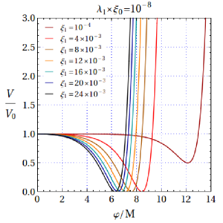
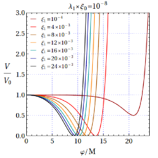
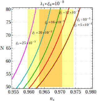
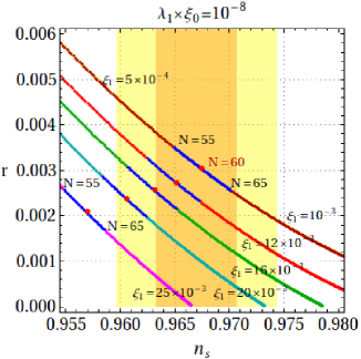
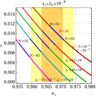
Figure 1: Left column: Weyl inflation plots; Right column: Palatini inflation plots. All figures have $\lambda_{1}\xi_{0}=10^{-8}\leq\xi_{1}^{2}$; Top plots: the potential $V/V_{0}$ in terms of $\varphi/M$ for different $\xi_{1}$; larger $\xi_{1}$ moves the curves to the left; larger $\lambda_{1}\xi_{0}$ lifts the minimum of the rightmost curves, see eq.(17); middle plots: the plots $(n_{s},N)$ for different $\xi_{1}$; bottom plots: the plots $(n_{s},r)$ for different $\xi_{1}$; curves of $\xi_{1}=5\times 10^{-4}$ and $10^{-3}$ are degenerate; along these curves the value of $N$ changes: the blue line segment has points of $55\leq N\leq 65$; red dots have $N=60$. The yellow (orange) area corresponds to the measured value of $n_{s}$ at $95\%$ CL $(68\%)$, respectively.

3 Inflation

3.1 Weyl versus Palatini

We can now use Lagrangian (16) and potential $V(\varphi)$ of (17) to study inflation with $\varphi$ as the inflaton and compare its predictions for the Weyl ($\gamma=1/4$) and Palatini ($\gamma=1$) cases. For a previous study of inflation in the Weyl case, see [70, 7]. Lagrangian (16) describes a single scalar field in Einstein gravity and the usual formalism for a single-field inflation can be used. However, notice there exists a coupling of $\varphi$ to the Weyl field $\hat{w}_{\mu}$, the second term in (16). Hence, we must first show that this coupling and $\hat{w}_{\mu}$ do not affect inflation by $\varphi$.

Firstly, we do not consider here the possibility of the Weyl vector field itself as the inflaton since it could induce a substantial large-scale anisotropy [73] which would be in conflict with CMB isotropy. The anisotropy is obvious in the stress-energy tensor contribution of $\hat{w}_{\mu}$ which is not diagonal. This issue can be avoided if one considers a large number of randomly oriented vector fields or a triplet of mutually orthogonal vector fields [73], however this is not possible in the current fixed setup.

Secondly, one may ask if the Weyl field could play the role of a curvaton with $\varphi$ as the inflaton. The scenario of a vector field as a curvaton was discussed in detail in [74, 75]; in such scenario the vector field does not drive inflation (to avoid large scale anisotropy) but becomes important after inflation when it may dominate the Universe and imprint its perturbation spectrum. A scale invariant spectrum can be generated by $\hat{w}_{\mu}$ provided that during inflation the mass-squared of $\hat{w}_{\mu}$ is negative and large in absolute value ($\sim\!H^{2}$) while after inflation is positive and the vector field engages in oscillations and behaves as pressureless matter; this means it does not lead to large-scale anisotropy when it dominates [74, 75]. This scenario cannot apply here since $m^{2}_{w}$ is always positive. Indeed, the second term in (16)

$$\Delta L=\frac{1}{2}\sqrt{\hat{g}}f(\varphi)\,\hat{w}_{\mu}\hat{w}^{\mu},\qquad f(\varphi)=6\gamma M^{2}\cosh^{2}\frac{\varphi}{2M\sqrt{\gamma}}.$$ (19)

has $f(\varphi)>0$, for any value of $\varphi$ and the effective mass-squared of $\hat{w}_{\mu}$ is always positive.

Finally, in Friedmann-Robertson-Walker (FRW) universe $\hat{g}_{\mu\nu}\!=\!(1,-a(t)^{2},-a(t)^{2},-a(t)^{2}$, the vector field background compatible with the metric is $\hat{w}_{\mu}(t)\!=\!(\hat{w}_{0}(t),0,0,0)$. However, from the equation of motion of $\hat{w}_{\mu}$ one immediately sees that $\hat{w}_{\mu}(t)\!=\!0$, (see also eq.(C-13) for details). In this case $\Delta L$ is vanishing. Therefore, we are left with potential (17) and the usual formalism of single-field inflation in Einstein gravity applies, with $\varphi$ as inflaton.

One may ask what happens at the perturbations level? One easily sees that perturbations $\delta\varphi$ of $\varphi$ do not mix with perturbations $\delta\hat{w}_{\mu}$ (of longitudinal mode/Stueckelberg field $\rho$) of massive $\hat{w}_{\mu}$. Such mixing is in principle possible, with potential impact on inflation predictions, but it vanishes since it is proportional to $\hat{w}_{\mu}(t)(=0)$, as seen from expanding $\Delta L$ to quadratic level in perturbations: $\Delta L\propto\hat{w}^{\mu}(t)\,\delta\varphi\,\delta\hat{w}_{\mu}+\cdots$ . As a result, the coupling $\Delta L$ does not affect $\delta\varphi$ and the predictions of inflation by $\varphi$. For further discussion on perturbations $\delta\varphi$ and $\delta\hat{w}_{\mu}$ see Appendix C which supports these results.

The above arguments justify our use below of single-field slow-roll formulae

$$\epsilon = \frac{M^{2}}{2}\Big{\{}\frac{V^{\prime}(\varphi)}{V(\varphi)}\Big{\}}^{2}=\frac{{4}}{3}\,\gamma\,\xi_{1}^{2}\,\sinh^{2}\frac{\varphi}{M\sqrt{6\gamma}}+{\cal O}(\xi_{1}^{3}),\,$$ (20)

$$\eta = M^{2}\,\frac{V^{\prime\prime}(\varphi)}{V(\varphi)}=-\frac{2}{3}\,\xi_{1}\,\cosh{\frac{\varphi}{M\sqrt{6\gamma}}}+\frac{8}{3}\gamma\,\xi_{1}^{2}\sinh^{2}\frac{\varphi}{2M\sqrt{6\gamma}}+{\cal O}(\xi_{1}^{3}),\,$$ (21)

The number of e-folds is

$$N=\frac{1}{M^{2}}\int_{\varphi_{e}}^{\varphi_{*}}d\varphi\,\,\frac{V(\varphi)}{V^{\prime}(\varphi)}=\Big{\{}-\frac{3}{4\,\xi_{1}}\ln\tanh^{2}\frac{\varphi}{2M\sqrt{6\gamma}}+3\gamma\ln\cosh^{2}\frac{\varphi}{2M\sqrt{6\gamma}}\Big{\}}\Big{|}_{\varphi=\varphi_{e}}^{\varphi=\varphi_{*}}.$$ (22)

with the last step in (20), (21), (22) valid in the leading approximation $\lambda_{1}\xi_{0}\ll\xi_{1}^{2}$ needed for a deep enough minimum for inflation; $\varphi_{e}$ is determined by $\epsilon(\varphi_{e})=1$ and $\varphi_{*}$ is the initial value of the scalar field. Further, the scalar spectral index

$$n_{s}\,=\,1+2\,\eta_{*}-6\,\epsilon_{*}=1-\frac{4}{3}\,\xi_{1}\,\cosh\frac{\varphi_{*}}{M\sqrt{6\gamma}}+\frac{8}{3}\,\xi_{1}^{2}\,\gamma\,\Big{[}\cosh^{2}\frac{\varphi_{*}}{M\sqrt{6\gamma}}-1\Big{]}+{\cal O}(\xi_{1}^{3}).\,$$ (23)

With the tensor-to-scalar ratio $r=16\epsilon_{*}$, then from (20), (21), (23)

$$r={12}\,\gamma\,(1-n_{s})^{2}-\frac{64\gamma}{3}\,\xi_{1}^{2}+{\cal O}(\xi_{1}^{3}).$$ (24)

The non-minimal coupling is reducing $r$, for fixed $n_{s}$. If we ignore the term $\propto\xi_{1}^{2}$ and higher orders, then the Palatini case ($\gamma=1$) has a larger $r$ than Weyl theory ($\gamma=1/4$), for the same $n_{s}$. This is confirmed by exact numerical results, see later. From (22), we also find

$$r\approx\frac{48\gamma}{\overline{N}^{2}}+\frac{64\gamma}{\overline{N}}\times O(\xi_{1});\qquad n_{s}\approx 1-\frac{2}{\overline{N}}+{\cal O}(\xi_{1})$$ (25)

with $\overline{N}\approx N+9$ and $\gamma=1/4$ in the Weyl case and $\overline{N}\approx N+28$ and $\gamma=1$ for the Palatini case. Eqs.(25) are only an approximation and ignore some $\xi_{1}$ dependence in $\overline{N}$, but give an idea of the exact behaviour (see later, Figure 2).

There is an additional constraint on the parameters space of Weyl/Palatini models, from the normalization of the CMB anisotropy $V_{0}/(24\pi^{2}M^{4}\epsilon_{*})=\kappa_{0}$, $\kappa_{0}=2.1\times 10^{-9}$ and with $r<0.07$ [78] then $\xi_{0}=1/(\pi^{2}r\kappa)\geq 6.89\times 10^{8}$. With this bound, condition $\lambda_{1}\xi_{0}\!\ll\!\xi_{1}^{2}$ is respected for any perturbative $\xi_{1}$, $1/\xi_{0}$, by choosing an ultraweak $\lambda_{1}\!\ll\!\xi_{1}^{2}/\xi_{0}$.

Let us compare eq.(24) to that in the Starobinsky model of

$${\cal L}=(-1/2)M^{2}\,R+(\xi_{0}/4!)\,R^{2},$$ (26)

giving $V\!=\!V_{0}\big{(}1-e^{-\varphi\sqrt{2/3}/M}\,\big{)}^{2}$ with $V_{0}\!=\!3M^{4}/(2\xi_{0})$; then $r\!\approx\!12/N^{2}$, $n_{s}\!\approx\!1-2/N$ and

$$r=3\,(1-n_{s})^{2}.$$ (27)

Interestingly, in eq.(24) with $\xi_{1}\!\sim\!10^{-3}$ or smaller, the term $\propto\xi_{1}^{2}$ and higher powers have a negligible correction to $r$ and $(1-n_{s})^{2}$ and can be ignored; therefore Weyl inflation ($\gamma=1/4$) recovers relation (27) of Starobinsky model [29, 78]. For larger values of $\xi_{1}$ and fixed $n_{s}$, $\xi_{1}$ reduces $r$ of Weyl inflation below that of Starobinsky model. In the Palatini case relation (27) is not possible (unless $\xi_{1}$ is tuned for every $n_{s}$) - the slope of $r(n_{s})$ is different.

3.2 Numerical results

Our exact numerical results (with no expansion in powers of $\xi_{1}$) are given by the plots of potential, $(n_{s},N)$, $(n_{s},r)$, presented in figures 1 and 2 for Weyl and Palatini cases. Their differences are due to different $\gamma$. The results show a value of $r$ smaller in the Weyl case than in Palatini case, for relevant $n_{s}$. For $n_{s}=0.9670\pm 0.0037\,(68\%{\rm CL})$ (TT, TE, EE + low E + lensing + BK14 +BAO) [78] one finds

$$\!\!\!\!{\rm Palatini:} \!\!\!\!\!N=60,\quad 0.00794\leq r\leq 0.01002,\quad$$ (28)

$${\rm Weyl:} \!\!\!\!\!N=60,\quad 0.00257\leq r\leq 0.00303.$$ (29)

and for $n_{s}$ at $95\%{\rm CL}$ one has

$$\!\!\!\!{\rm Palatini:} \!\!\!\!\!N=60,\quad 0.00700\leq r\leq 0.01002,\quad$$ (30)

$${\rm Weyl:} \!\!\!\!\!N=60,\quad 0.00227\leq r\leq 0.00303.$$ (31)

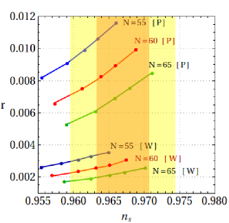
Figure 2: The dependence $r(n_{s})$ for various curves of constant $N$ (as shown), for the Palatini theory ([P]) and Weyl theory ([W]). The dots stand for $\xi_{1}$ values corresponding to the curves in the last two plots in Figure 1. The yellow (orange) area corresponds to the range measured for $n_{s}$ at $95\%$CL $(68\%)$, respectively. The curves show the largest range of values for $r$ with $\lambda_{1}\xi_{0}\ll\xi_{1}^{2}$; this range shrinks towards smaller $r$ if $\lambda_{1}\xi_{0}$ increases to $\lambda_{1}\xi_{0}\sim\xi_{1}^{2}$.

The case of Starobinsky model for $N=60$ corresponds to the upper limit of $r$ (0.003) of the Weyl model (top curve in figure 1 and highest $r$ in figure 2 for $N=60$), while in the Palatini case a larger $r$ is allowed for the same $n_{s}$, $N$.

While the plots in figure 1 have $\lambda_{1}\xi_{0}=10^{-8}$, they are actually more general. In the extreme case of $\lambda_{1}\!\sim\!0$, corresponding to a simplified potential (without the last term in (17)), the same range of values for $(n_{s},r)$ shown in this figure remains valid. However, if we increase $\lambda_{1}\xi_{0}$ to $\lambda_{1}\xi_{0}\approx\xi_{1}^{2}$, the last term in (17) becomes relatively large, the rightmost curves of $V$ (of smallest $\xi_{1}$) have their minimum lifted and the range for $(n_{s},r)$ in (28) to (31) is reduced: the smaller values $\xi_{1}\!\sim\!10^{-3}$ in Figure 1, cannot then have successful inflation.

The main results of this work are summarised in figure 2; in this figure the dependence $r(n_{s})$ is shown for different curves of constant $N$, that respect the required parametric constraint $\lambda_{1}\xi_{0}\leq\xi_{1}^{2}$. The curves $r(n_{s})$ give a numerically exact representation of the dependence in eq.(24); they are extended even outside the $95\%$ CL range for $n_{s}$. In all cases, the Palatini case has $r$ larger than in the Weyl case. This aspect and the different slope of the curves $r(n_{s})$ can be used to distinguish these models from each other and from other models in future experiments.

The small $r$ predicted by both Weyl and Palatini gravity models may be reached by the next generation of CMB experiments: CMB-S4, LiteBIRD, PICO, PIXIE [79, 83, 81, 82, 84, 80] that will reach a precision for $r$ of $\sim 5\times 10^{-4}$. Therefore they will be able to test these two inflation models.

3.3 Corrections and other models

Compared to another model with Weyl gauge symmetry [27] (figure 2) which is linear in $R(\tilde{\Gamma},g)$ and had $r\sim 0.04-0.06$, we see that the presence of the $R^{2}(\tilde{\Gamma},g)$ term in the Weyl theory reduced $r$ significantly (for a fixed $n_{s}$). Reducing $r$ by an $R^{2}$ term also exists in the Palatini models without Weyl gauge symmetry [64]. Therefore, a small measured $r\!\sim\!10^{-3}$ may indicate a preference for quadratic gravity models of inflation.

The Weyl inflation case of $\xi_{1}=10^{-3}$ or smaller is similar to the Starobinsky model. Here we have an additional scalar field, with $\varphi$ playing the role of the inflaton. The other scalar in the Weyl theory (radial direction $\rho$ in the $\phi_{0}$, $\phi_{1}$ space) is used to generate the Planck scale and the mass of $w_{\mu}$. Briefly, Weyl gravity gives a relation $r(n_{s})$ similar to that in the Starobinsky model, with similar, large $\xi_{0}$, while also providing protection against corrections to $r$ from higher dimensional operators; these are forbidden since their effective scale violates the symmetry; the Stueckelberg field cannot play the role of this scale since it was eaten by the Weyl field to all orders. Another benefit for Weyl inflation is the minimal approach: one only needs to consider the SM Higgs field in the Weyl conformal geometry; the underlying geometry provides the spontaneous breaking of the Weyl quadratic gravity action to the Einstein action and the Planck scale generation.

Despite this similarity of the Weyl and the Starobinsky models, it is possible to distinguish between them; it may happen that a curve $r(n_{s})$ corresponding to $\xi_{1}>10^{-3}$ is preferred by data (see $r(n_{s})$ curves in figure 1), in which case it is shifted below that of the Starobinsky model for the same $n_{s}$ - the two models are distinguishable. Also the Weyl model has an additional coupling, see $\Delta L$ in (19). While $\Delta L$ does not mix linear perturbations of $\delta w_{\mu}$ and of $\delta\varphi$, it can lead however to cubic interactions of the form $f^{\prime}(\varphi)\delta\varphi\delta w_{\mu}\delta w^{\mu}$. These can result in different predictions for the inflationary bispectrum compared to the pure single-field case. This can be used to further distinguish the Weyl case from the Starobinsky $R^{2}$ inflation (for $\xi_{1}\sim 10^{-3}$). The analysis of non-Gaussianity is thus interesting for further research.

The above results are subject to corrections from other operators of $d=4$ that may exist and are Weyl gauge invariant, as we discuss below.

In the Weyl case the Weyl-tensor-squared operator of Weyl geometry may be present $(1/\zeta)\tilde{C}_{\mu\nu\rho\sigma}^{2}$. This can be re-written in a metric description as the Weyl-tensor-squared term of Riemannian geometry $(1/\zeta)\,C_{\mu\nu\rho\sigma}^{2}$ plus a gauge kinetic term of $w_{\mu}$ which gives a threshold correction to our coupling $\alpha$. The Weyl tensor term is invariant under Weyl gauge transformations performed to reach the Einstein-Proca action, hence one simply adds it to the final action, eq.(14). This operator has an impact on the value of $r$ that we found numerically and in eq.(25) with $\gamma=1/4$ for Weyl case. The overall impact of the Weyl tensor term is essentially a rescaling of $r$ into $r_{c}=r\,(1+8/(\zeta\,\xi_{0}))^{1/2}$ [7]. Since our $\xi_{0}$ is large, only a low $|\zeta|\sim 1/\xi_{0}$ can increase $r$ and this comes with an instability since the mass of the associated spin-two ghost (or tachyonic) state that this operator brings is $m^{2}\sim\zeta\,M^{2}$, where $M$ is the Planck scale. Therefore, a stable Weyl gravity model up to the Planck scale will not modify the value of $r$. Other operators in Weyl gravity are topological and do not affect $r$ (classically).

In the Palatini case one should consider the remaining quadratic operators of $d=4$ [85] that are Weyl gauge invariant and have a symmetric connection. They modify the equation of motion of $\tilde{\Gamma}$ and the vectorial non-metricity (B-6); unfortunately, it does not seem possible to find in this case an analytical solution to this equation due to its modified, complex structure and new states present (ghosts, etc). Additional simplifying assumptions would be needed, making the analysis model dependent. We only mention here the interesting possibility that for a symmetric $\tilde{\Gamma}$, the solution $\tilde{\Gamma}$ may become equal to that in Weyl-geometry (A-5); if so, the Palatini approach would provide an “offshell” version of Weyl quadratic gravity that is recovered for $\tilde{\Gamma}$ onshell.

4 Conclusions

We made a comparative study of the action and inflation in two theories of quadratic gravity with Weyl gauge symmetry: the original Weyl gravity action and the Palatini version of the same action, obtained by replacing the Weyl connection by Palatini connection. The actions of these theories are non-minimally coupled to a (Higgs-like) field $\phi_{1}$.

Given the symmetry, there is no scale in these theories. Mass scales are generated by an elegant spontaneous breaking of gauged scale symmetry that happens even in the absence of matter: the necessary scalar field (Stueckelberg field $\phi_{0}$) is not added ad-hoc as usually done to this purpose, but is of geometric origin and is ”extracted” from the $R(\tilde{\Gamma},g)^{2}$ term in the action. If matter ($\phi_{1}$) is present, the Stueckelberg field is actually the radial direction ($\rho$) in the field space of $\phi_{0}$ and $\phi_{1}$; the field $\rho$ is then eaten by the Weyl gauge field $w_{\mu}$ which acquires mass $m_{w}\sim\langle\rho\rangle$ near the Planck scale. The breaking conserves the number of degrees of freedom and generates in the broken phase the Einstein-Proca action for $w_{\mu}$. In both theories, below the mass of $w_{\mu}$ the connection becomes Levi-Civita and Einstein gravity is recovered, with an “emergent” Planck scale $M\sim\langle\rho\rangle$ and a scalar potential (of the remaining, angular-variable field $\varphi$).

The potential $V(\varphi)$ is controlled by the symmetry of the theory together with effects from the non-trivial connection $\tilde{\Gamma}$, different in the two theories. For small field values, $V$ is similar in both theories; the scalar field can act as the Higgs field, in which case the potential displays electroweak symmetry breaking. For large field values, the potential has the same form in Weyl and Palatini theories up to couplings and field rescaling (due to different non-metricity) and gives successful inflation.

Our main results, comparing inflation predictions in the two theories and summarised in Figure 2, showed how a different non-metricity impacts on inflation predictions. In Weyl gravity the scalar-to-tensor ratio $0.00257\!\leq\!r\!\leq\!0.00303$, which is smaller than in Palatini case, $0.00794\!\leq\!r\!\leq\!0.01002$, for measured $n_{s}$ at 68$\%$ CL and $N=60$ e-folds. Similar results exist for $n_{s}$ at $95\%$CL or mildly different $N$, etc. Such values of $r$ will be measured by new CMB experiments that can then test and distinguish Weyl and Palatini quadratic gravity.

There are similarities of inflation in Weyl and Palatini cases to Starobinsky inflation ($R+\xi_{0}R^{2}$). In Weyl and Palatini theories one also has an $R^{2}$ term with a large $\xi_{0}$ that reduces $r$, but there is also a non-minimally coupled scalar field ($\phi_{1}$); one combination of fields is acting as the inflaton while the other (radial) combination enabled the breaking of the gauged scale symmetry and the generation of mass scales (Planck, $w_{\mu}$ mass). In both Weyl and Palatini theory, for a fixed $n_{s}$, reducing the non-minimal coupling ($\xi_{1}$) increases $r$ which in Weyl theory is bounded from above by that of Starobinsky inflation. Unlike in the Palatini theory, Weyl gravity for $\xi_{1}\leq 10^{-3}$ gives a dependence $r(n_{s})$ essentially similar to that in Starobinsky inflation, while also protecting $r$ against higher dimensional operators corrections.

—————————

Appendix

A Weyl gravity

We include here basic information on Weyl gravity used in the text. First, in the (pseudo)-Riemannian case (Einstein gravity) $\nabla_{\mu}g_{\alpha\beta}\!=\!0$ with $\nabla_{\mu}$ defined by the Levi-Civita connection

$$\Gamma_{\mu\nu}^{\rho}(g)=(1/2)\,g^{\rho\beta}\,(\partial_{\nu}g_{\beta\mu}+\partial_{\mu}g_{\beta\nu}-\partial_{\beta}g_{\mu\nu}).$$ (A-1)

Setting $\nu=\rho$ and summing over gives $\Gamma_{\mu}\equiv\Gamma_{\mu\nu}^{\nu}=\partial_{\mu}\ln\sqrt{g}$ used in the text.

In Weyl gravity and conformal geometry the theory has vectorial non-metricity, i.e.

$$\tilde{\nabla}_{\lambda}\,g_{\mu\nu}=-w_{\lambda}\,g_{\mu\nu},$$ (A-2)

so $w_{\lambda}=(-1/4)\,g^{\mu\nu}\,\tilde{\nabla}_{\lambda}g_{\mu\nu}$; here $\tilde{\nabla}_{\mu}$ is defined by the Weyl connection $\tilde{\Gamma}_{\mu\nu}^{\rho}$:

$$\tilde{\nabla}_{\lambda}g_{\mu\nu}=\partial_{\lambda}g_{\mu\nu}-\tilde{\Gamma}_{\mu\lambda}^{\rho}g_{\rho\nu}-\tilde{\Gamma}_{\nu\lambda}^{\rho}g_{\mu\rho}.$$ (A-3)

Write this for cyclic permutations of the indices and combine the three equations to find

$$\tilde{\Gamma}_{\mu\nu}^{\rho}=\Gamma_{\mu\nu}^{\rho}(g)+(1/2)\,g^{\rho\lambda}\,(\tilde{\nabla}_{\lambda}g_{\mu\nu}-\tilde{\nabla}_{\mu}g_{\nu\lambda}-\tilde{\nabla}_{\nu}g_{\lambda\mu}),$$ (A-4)

which with (A-2) gives the Weyl connection

$$\tilde{\Gamma}_{\mu\nu}^{\rho}=\Gamma_{\mu\nu}^{\rho}(g)+(1/2)\,\big{[}\delta_{\mu}^{\rho}\,w_{\nu}+\delta_{\nu}^{\rho}\,w_{\mu}-g_{\mu\nu}\,w^{\rho}\big{]}.$$ (A-5)

$\tilde{\Gamma}_{\mu\nu}^{\rho}$ are symmetric ($\tilde{\Gamma}_{\mu\nu}^{\rho}=\tilde{\Gamma}_{\nu\mu}^{\rho}$) i.e. there is no torsion. $\tilde{\Gamma}$ is invariant under transformations (2), (3) since the variation of the metric is compensated by that of $w_{\mu}$. Using that $g^{\alpha\beta}\tilde{\nabla}_{\lambda}g_{\alpha\beta}=2\tilde{\nabla}_{\lambda}\ln\sqrt{g}$ one finds for the Weyl field

$$w_{\lambda}=(-1/2)\,\,\tilde{\nabla}_{\lambda}\ln\sqrt{g}.$$ (A-6)

Setting $\nu=\rho$ in (A-5) and summing over, we recover our definition (3) in the text:

$$\tilde{\Gamma}_{\mu}=\Gamma_{\mu}(g)+2\,w_{\mu}.$$ (A-7)

The Riemann and Ricci tensors in Weyl geometry are defined as in Riemannian geometry but with the replacement of the Levi-Civita connection $\Gamma_{\mu\nu}^{\rho}(g)$ by the new $\tilde{\Gamma}_{\mu\nu}^{\rho}$

$$R^{\lambda}_{\,\mu\nu\sigma}(\tilde{\Gamma},g)=\partial_{\nu}\tilde{\Gamma}^{\lambda}_{\mu\sigma}-\partial_{\sigma}\tilde{\Gamma}^{\lambda}_{\mu\nu}+\tilde{\Gamma}^{\lambda}_{\nu\rho}\,\tilde{\Gamma}^{\rho}_{\mu\sigma}-\tilde{\Gamma}^{\lambda}_{\sigma\rho}\,\tilde{\Gamma}^{\rho}_{\mu\nu},$$ (A-8)

and

$$R_{\mu\sigma}(\tilde{\Gamma},g)=R^{\lambda}_{\,\,\mu\lambda\sigma}(\tilde{\Gamma},g),\qquad R(\tilde{\Gamma},g)=g^{\mu\sigma}\,{\tilde{R}}_{\mu\sigma}(\tilde{\Gamma},g).$$ (A-9)

Since $\tilde{\Gamma}$ is invariant under transformations (2), (3), then the Riemann and Ricci tensors of Weyl geometry are also invariant. Since the Weyl scalar curvature $R(\tilde{\Gamma},g)$ contains $g^{\mu\nu}$, it transforms covariantly

$$\hat{R}(\tilde{\Gamma},g)=(1/\Omega^{2})\,R(\tilde{\Gamma},g).$$ (A-10)

This helps build Weyl gauge invariant operators. Using the expression of $\tilde{\Gamma}$, one shows

$$R(\tilde{\Gamma},g)=R(g)-3\,\nabla_{\mu}w^{\mu}-\frac{3}{2}\,g^{\mu\nu}\,w_{\mu}w_{\nu},$$ (A-11)

where $R(g)$ is the Riemannian scalar curvature and $\nabla_{\mu}w^{\mu}$ is defined by Levi-Civita connection. Eq.(A-11) was used in the text, in going from (10) to (12) for the Weyl case.

B Palatini gravity

We present here the connection and the scalar curvature for the Palatini approach to gravity, used in the text. In this case, similarly to Weyl gravity, $\tilde{\Gamma}$ is not determined by the metric (apriori is independent of it), hence it is invariant under rescaling $g_{\mu\nu}$. The connection is determined by its equation of motion from the Lagrangian of eq.(10). Solving this equation of motion one finds [8] (eqs.23, 25, 39)

$$\tilde{\nabla}_{\lambda}(\rho^{2}g_{\mu\nu})=(-2)\rho^{2}(g_{\mu\nu}\,V_{\lambda}-g_{\mu\lambda}V_{\nu}-g_{\nu\lambda}V_{\mu}),$$ (B-1)

where $V_{\lambda}$ is some arbitrary vector, related to $w_{\lambda}$ (see below). One writes (B-1) for cyclic permutations of the three indices, then combines the equations obtained and uses the symmetry $\tilde{\Gamma}_{\mu\nu}^{\alpha}=\tilde{\Gamma}_{\nu\mu}^{\alpha}$, to find

$$\tilde{\Gamma}_{\mu\nu}^{\alpha} = \Gamma_{\mu\nu}^{\alpha}(\rho^{2}g)-\,\big{(}3\,g_{\mu\nu}\,V_{\lambda}-g_{\nu\lambda}\,V_{\mu}-g_{\lambda\mu}\,V_{\nu}\,\big{)}\,g^{\lambda\alpha},$$ (B-2)

where

$$\Gamma^{\alpha}_{\mu\nu}(\rho^{2}g)=\Gamma^{\alpha}_{\mu\nu}(g)+1/2\,\big{(}\delta_{\nu}^{\alpha}\,\partial_{\mu}+\delta_{\mu}^{\alpha}\,\partial_{\nu}-g^{\alpha\lambda}g_{\mu\nu}\,\partial_{\lambda})\ln\rho^{2},$$ (B-3)

with $\Gamma_{\mu\nu}^{\alpha}(g)$ the Levi-Civita connection for $g_{\mu\nu}$. Setting $\nu\!=\!\alpha$ in (B-2) one then finds $\tilde{\Gamma}_{\mu}\!=\Gamma_{\mu}(\phi^{2}g)+2\,V_{\mu}$ and from (B-3): $\Gamma_{\mu}(\phi^{2}g)=\Gamma_{\mu}(g)+2\,(\partial_{\mu}\ln\rho^{2})$. From these two equations and with the definition $w_{\lambda}=1/2\,(\tilde{\Gamma}_{\mu}-\Gamma_{\mu}(g))$, then $V_{\lambda}=w_{\lambda}-\partial_{\lambda}\ln\rho^{2}$. Using this relation and that found by contracting (B-1) by $g^{\mu\nu}$, then

$$w_{\lambda}=(-1/2)\tilde{\nabla}_{\lambda}\ln\sqrt{g}.$$ (B-4)

similar to (A-6), but with different $\tilde{\Gamma}$. Finally, eqs.(B-2), (B-3) together with $V_{\lambda}=w_{\lambda}-\partial_{\lambda}\ln\rho^{2}$, give the expression of $\tilde{\Gamma}$ in terms of $g_{\mu\nu}$, $\rho$ and $w_{\lambda}$ and verifies that $\tilde{\Gamma}$ is indeed invariant under a gauged scale transformation (2), (3). This is obvious since $\rho^{2}g_{\mu\nu}$ and $V_{\mu}$ are invariant in (B-2). With $\tilde{\Gamma}$ a function of $w_{\lambda}$, $\phi$, $g_{\mu\nu}$, one computes the Ricci tensor $R_{\mu\nu}(\tilde{\Gamma})$ for Palatini gravity, then the scalar curvature $R(\tilde{\Gamma},g)=g^{\mu\nu}R_{\mu\nu}(\tilde{\Gamma},g)$. The result is [8]:

$$R(\tilde{\Gamma},g)=R(g)-6g^{\mu\nu}\nabla_{\mu}\nabla_{\nu}\ln\rho-6(\nabla_{\mu}\ln\rho)^{2}-12\,\big{(}\nabla_{\lambda}V^{\lambda}+V^{\lambda}\partial_{\lambda}\ln\rho^{{2}}\big{)}-6V_{\mu}\,V^{\mu},$$ (B-5)

with $R(g)$ the Ricci scalar (Riemannian case), and $V_{\lambda}\equiv w_{\lambda}-\partial_{\lambda}\ln\rho^{2}$. Replacing (B-5) in eq.(10) for the Palatini case, one finds after some algebra eq.(12) in the text with $\gamma=1$. At the same time, the vectorial non-metricity becomes

$$\tilde{\nabla}_{\lambda}g_{\mu\nu}=(-2)\,(g_{\mu\nu}w_{\lambda}-g_{\mu\lambda}w_{\nu}-g_{\nu\lambda}w_{\mu}),$$ (B-6)

which is different from (A-2) of Weyl geometry, but has the same trace $g^{\mu\nu}\tilde{\nabla}_{\lambda}g_{\mu\nu}=-w_{\lambda}/4$.

C Inflation: perturbations to the scalar and vector fields

We discuss in detail the scalar ($\delta\phi$) and vector ($\delta w_{\mu}$) fields perturbations in a FRW universe $g_{\mu\nu}\!=\!(1,-a(t)^{2},-a(t)^{2},-a(t)^{2})$ and show that $\Delta L$ of (19) does not affect inflation by $\varphi$. To simplify notation hereafter we remove the ’hat’ ($\hat{\,}$) on $w_{\mu}$, $g_{\mu\nu}$ when we refer to action (16).

$\bullet$ Let us first review the usual case of a single scalar field, see e.g.[76], needed later. Consider

$${\cal L}_{\varphi}=\int\sqrt{g}\Big{[}\frac{1}{2}\,g^{\mu\nu}\,\partial_{\mu}\varphi\partial_{\nu}\varphi-\mathcal{V}(\varphi)\Big{]}.$$ (C-1)

The equation of motion $\nabla_{\mu}\nabla^{\mu}\varphi+\mathcal{V}^{\prime}(\varphi)=0$ gives for a FRW metric:

$$\ddot{\varphi}(\vec{x},t)+3H\dot{\varphi}(\vec{x},t)-\frac{1}{a(t)^{2}}\partial_{j}\partial_{j}\varphi(\vec{x},t)+{\mathcal{V}}^{\prime}(\varphi)=0$$ (C-2)

Expanding about $\varphi(t)$, with $\varphi(\vec{x},t)=\varphi(t)+\delta\varphi(\vec{x},t)$, one has at linear level

$$\delta\ddot{\varphi}(\vec{x},t)+3H\delta\dot{\varphi}(\vec{x},t)-\frac{1}{a(t)^{2}}\partial_{j}\partial_{j}\delta\varphi(\vec{x},t)+{\mathcal{V}}^{\prime\prime}(\varphi(t))\delta\varphi(\vec{x},t)=0$$ (C-3)

Using mode expansion $\delta\varphi(\vec{x},t)=\int d^{3}k/(2\pi)^{3/2}\delta\varphi_{k}(t)\exp(i\vec{x}\vec{k})$, then

$$\delta\ddot{\varphi}_{k}+3H\delta\dot{\varphi}_{k}+\big{[}k^{2}/a^{2}+{\mathcal{V}}^{\prime\prime}(\varphi(t))\big{]}\delta\varphi_{k}=0$$ (C-4)

or, with a notation $\delta\phi_{k}=\delta\chi_{k}/a(t)$

$$\delta\ddot{\chi}_{k}+H\delta\dot{\chi}_{k}+\big{[}k^{2}/a^{2}-\dot{H}-2H^{2}+{\mathcal{V}}^{\prime\prime}(\varphi(t))\big{]}\delta\varphi_{k}=0.$$ (C-5)

In conformal time ($\eta$) via $dt=a(t)^{2}d\eta$, this equation becomes

$$\delta\chi^{\prime\prime}_{k}+\big{[}k^{2}-(1/\eta^{2})\,(\nu^{2}-1/4)\big{]}\delta\varphi_{k}=0,\qquad\nu^{2}=9/4-{\mathcal{V}}^{\prime\prime}/H^{2}.$$ (C-6)

where we used that with $a\sim e^{Ht}$ then $a(\eta)=-1/(H\eta)$ and $2/\eta^{2}=a^{\prime\prime}/a$ with $H\sim$constant. In the subhorizon limit $-\eta\,k\gg 1$ the solution should be $\delta\chi_{k}=e^{-ik\eta}/\sqrt{2k}$. With this boundary condition, the solution is

$$\delta\chi_{k}=\frac{\sqrt{\pi}}{2}e^{i(\nu+1/2)\pi/2}\sqrt{-\eta}\,H_{\nu}^{(1)}(-\eta k)$$ (C-7)

where $H^{(1)}$ is the Hankel function of first kind. This leads to the usual power spectrum, with

$$|\delta\phi_{k}|^{2}\approx\frac{H^{2}}{2k^{3}}\Big{(}\frac{k}{aH}\Big{)}^{2\eta_{\phi}},\qquad P_{\delta\phi_{k}}=\frac{k^{3}}{2\pi^{2}}|\delta\phi_{k}|^{2}=\Big{(}\frac{H}{2\pi}\Big{)}^{2}\,\Big{(}\frac{k}{aH}\Big{)}^{2\eta_{\phi}}$$ (C-8)

with $\eta_{\phi}=3/2-\nu\approx{\mathcal{V}}^{\prime\prime}/(3H^{2})=M_{p}^{2}\,{\mathcal{V}}^{\prime\prime}/{\mathcal{V}}\ll 1$. This gives $n_{\phi}=1+2\eta_{\phi}$ ($H\sim$ constant).

For later use, we also consider solution (C-7) when ${\mathcal{V}}^{\prime\prime}(\varphi)\!>\!(9/4)\,H^{2}$ i.e. $\nu$ is imaginary, $\nu=i\tilde{\nu}$, $\tilde{\nu}$ real. In the (superhorizon) limit $(-\eta\,k)\ll 1$ one finds:

$$\delta\chi_{k}=\frac{(1+i)\,2^{-3/2-i\tilde{\nu}}e^{-\tilde{\nu}\pi/2}}{\sqrt{\pi k}\Gamma(1+i\tilde{\nu})}\Big{[}\pi(-\eta k)^{2i\tilde{\nu}}(1+\coth\pi\tilde{\nu})+2^{2i\tilde{\nu}}\tilde{\nu}\,\Gamma(i\tilde{\nu})^{2}\Big{]}.$$ (C-9)

Returning to $\delta\phi_{k}$ notation, one finds (see e.g. [76])

$$P_{\delta\phi_{k}}=\frac{\pi e^{-\pi\tilde{\nu}}}{2}\frac{H^{2}}{(2\pi)^{2}}\Big{(}\frac{k}{aH}\Big{)}^{3}\,\{....\}$$ (C-10)

where the brackets $\{...\}$ stand for terms that vanish when $\tilde{\nu}\rightarrow\infty$ (${\mathcal{V}}^{\prime\prime}(\varphi)\gg H^{2}$). Therefore, modes $\delta\phi_{k}$ of $\nu$ imaginary are exponentially suppressed [77]; this is expected since they are too massive to be excited.

$\bullet$ Consider now our action (16); its $\varphi$-dependence is described by ${\cal L}_{\varphi}$ by replacing in (C-1)

$${\mathcal{V}}(\varphi)\rightarrow{\mathcal{V}}(\varphi,w)=V(\varphi)-\frac{1}{2}f(\varphi)w_{\mu}w^{\mu}$$ (C-11)

with $V(\varphi)$ of eq.(17) and $f(\varphi)$ of eq.(19). In this case (C-2) and the equation for $\varphi(t)$ receive a correction from the last term in the rhs of (C-11). Then eq.(C-4) for the perturbations $\delta\varphi_{k}$, also with $w_{\mu}(\vec{x},t)=w_{\mu}(t)+\delta w_{\mu}(\vec{x},t)$, is now modified into

$$\delta\ddot{\varphi}_{k}+3H\delta\dot{\varphi}_{k}+\big{[}k^{2}/a^{2}+{\mathcal{V}}^{\prime\prime}(\varphi(t),w(t))\big{]}\delta\varphi_{k}=f^{\prime}(\varphi(t))w_{\mu}(t)\delta w^{\mu}(\vec{k},t),$$ (C-12)

where the second derivative ${\mathcal{V}}^{\prime\prime}$ is with respect to $\varphi$ and $\delta w_{\mu}(\vec{k},t)$ are the Fourier modes of $\delta w_{\mu}(\vec{x},t)=\int d^{3}k/(2\pi)^{3/2}\delta w_{\mu}(\vec{k},t)\exp(i\vec{k}\vec{x})$. Next, the background $w_{\mu}(t)$ compatible with the FRW metric is $w_{\mu}(t)\!=\!(w_{0}(t),0,0,0)$, while from (16), the equation of motion of $w_{\mu}$ gives

$$\frac{1}{\sqrt{g}}\,\partial_{\rho}\,\big{[}\sqrt{g}\,F^{\rho\mu}\,\big{]}+f(\varphi)\,w^{\mu}=0.$$ (C-13)

One has a trivial solution $w_{\mu}(t)\!=\!0$ ($f(\varphi)\!\not=\!0$). Therefore, in (C-12) we must replace ${\mathcal{V}}^{\prime\prime}(\varphi(t),w(t))\rightarrow{\mathcal{V}}^{\prime\prime}(\varphi(t),0)=V^{\prime\prime}(\varphi)$ while the rhs of (C-12) is vanishing. Therefore equation (C-12) of $\delta\phi_{k}$ is actually independent of $w_{\mu}$ and $\delta w_{\mu}$ and there is no mixing of $\delta\varphi$ to $\delta w_{\mu}$ . Then the calculation of $\delta\varphi_{k}$ proceeds as earlier but for potential $V(\varphi)$, see (C-8) for ${\mathcal{V}}(\varphi)\!\rightarrow\!V(\varphi)$. Thus $\Delta L$ does not impact on $\varphi$-inflation and the usual formulae of single-field inflation in Einstein gravity apply, as used in Section 3.1.

$\bullet$ We saw above that the perturbations $\delta\varphi$ do not mix with those of $w_{\mu}$ and $\varphi$-inflation decouples from $w_{\mu}$ in a FRW universe. While somewhat beyond the purpose of this work, we also examine below the vector field perturbations, following [74, 75], in the approximation $H\sim$ constant. Compatibility with the FRW metric demands computing the perturbations about a background $w_{\mu}(t)=0$ as seen earlier. In fact we may take a more general background, if initially the vector field contribution to the stress-energy tensor is negligible relative to that of the scalar, in an isotropic universe; we shall then consider a quasi-homogeneous field $\partial_{i}w^{\alpha}=0$. Our FRW case is always restored by setting anywhere below $w_{\mu}(t)=0$. Then from (C-13) for $\mu=0$ and $\mu=i$, respectively

$$w_{0}(t)=0\quad\textrm{and}\quad\ddot{w}_{i}(t)+H\dot{w}_{i}(t)+f(\varphi)\,w_{i}(t)=0.$$ (C-14)

In an expanding FRW universe the relevant physical quantity is not $w_{i}$ ($i=1,2,3$) but $q_{i}=w_{i}/a$, as also seen from the norm $w_{\mu}w^{\mu}=w_{0}^{2}-(w_{i}w_{i})/a^{2}$ (sum over $i$) and from the stress energy tensor [73, 74]. Then the last equation becomes

$$\ddot{q}_{i}+3H\dot{q}_{i}+(2H^{2}+f(\varphi))\,q_{i}=0.$$ (C-15)

Denote $m^{2}=2H^{2}+f(\varphi(t))$ where $f(\varphi)>0$ since $f(\varphi(t))=6\gamma M^{2}\{1+\sinh^{2}[\varphi(t)/(2M\sqrt{\gamma})]\}$, eq.(19). Ignoring the time dependent part in $f(\varphi)$, the solution is

$$q_{i}(t)\propto 1/a(t)^{3/2}(c_{1}\,e^{-\alpha t/2}+c_{2}\,e^{\alpha t/2}),\qquad\alpha=\sqrt{H^{2}-4m^{2}}.$$ (C-16)

with constants $c_{1,2}$. Since $\alpha$ is purely imaginary, during inflation the vector field is massive with damped oscillations (up to corrections due to $\varphi(t))$). Its contribution to the stress energy tensor ($T^{\mu}_{\nu}$) is anisotropic; the spatial part of this tensor contains off-diagonal entries of comparable size to the diagonal ones and can be made diagonal for a particular direction of the vector field. However, with $q_{i}(t)\sim 1/a(t)^{3/2}$, the contribution of the vector field to $T^{\mu}_{\nu}$ during inflation is suppressed by the scale factor $1/a(t)^{3}$ relative to that of $\varphi$.

Consider now the equations for perturbations, with $w_{\mu}(\vec{x},t)=w_{\mu}(t)+\delta w_{\mu}(\vec{x},t)$. Then eqs.(C-13) for $\mu=i$ and $\mu=0$ give

$$\ddot{w}_{i}+H\,\dot{w}_{i}-\frac{1}{a(t)^{2}}\big{[}\partial_{j}\partial_{j}w_{i}-\partial_{i}\partial_{j}w_{j}\big{]}+f(\varphi)\,w_{i} = \partial_{i}\dot{w}_{0}+H\partial_{i}w_{0}$$ (C-18)

$$\partial_{i}\dot{w}_{i}-\partial_{i}\partial_{i}w_{0}+a(t)^{2}\,f(\varphi)w_{0} = 0$$ (C-19)

with $w_{\mu}=w_{\mu}(\vec{x},t)$ and $\varphi=\varphi(\vec{x},t)$. By applying $\partial_{\mu}$ on (C-13) we find

$$i\partial_{i}\dot{w}_{0}-\frac{1}{a(t)^{2}}\partial_{i}\partial_{j}w_{j}+3H\partial_{i}w_{0}+\partial_{i}D=0$$ (C-20)

where $D\!=\!D(\vec{x},t)$ and $D\!=\!w_{0}\partial_{0}\ln f(\varphi)-1/a(t)^{2}w_{j}\partial_{j}\ln f(\varphi)$. Adding (C-18), (C-20) then

$$\ddot{w}_{i}+H\dot{w}_{i}-\frac{1}{a(t)^{2}}\partial_{j}\partial_{j}w_{i}+f(\varphi)w_{i}=-2H\partial_{i}w_{0}-\partial_{i}D.$$ (C-21)

This gives for perturbations $\delta w_{\mu}$ a linear differential equation:

$$\delta\ddot{w}_{i}+H\delta\dot{w}_{i}-\frac{1}{a(t)^{2}}\partial_{j}\partial_{j}\delta w_{i}+f(\varphi(t))\delta w_{i}=-(2H+\partial_{0}\ln f(\varphi(t)))\partial_{i}\delta w_{0}-f^{\prime}(\varphi(t))w_{j}(t)\sigma_{ij}(t)$$ (C-22)

Here $\sigma_{ij}(\vec{x},t)=[\delta_{ij}+1/(a(t)^{2}f(\varphi(t)))\,\,\partial_{i}\partial_{j}]\,\delta\varphi(\vec{x},t)$; notice that in general case of $w_{i}(t)\not\!=\!0$ (C-22) is “mixing” $\delta\varphi$ and $\delta w_{\mu}$. However, this mixing is absent in our FRW case of $w_{\mu}(t)\!=\!0$.

Further, from remaining (C-19)

$$\partial_{i}\,\delta\dot{w}_{i}(\vec{x},t)-\partial_{i}\partial_{i}\,\delta w_{0}(\vec{x},t)+a(t)^{2}\,f(\varphi(t))\,\delta w_{0}(\vec{x},t)=0.$$ (C-23)

or, in Fourier modes

$$\delta w_{0}(\vec{k},t)=-i\frac{k_{j}\delta\dot{w}_{j}(\vec{k},t)}{k^{2}+a^{2}f(\varphi(t))}.$$ (C-24)

We separate the perturbations into parallel and orthogonal directions to $\vec{k}$ (taken along OZ):

$$\delta\vec{w}^{\parallel}=\frac{\vec{k}(k_{i}\delta w_{i})}{k^{2}},\qquad\delta\vec{w}^{\perp}=\delta\vec{w}-\delta\vec{w}^{\parallel}.$$ (C-25)

We introduce the physical perturbations $\delta q_{\mu}(\vec{x},t)=(1/a(t))\,\delta w_{\mu}(\vec{x},t)$ and express (C-22) in terms of the Fourier modes $\delta q_{\mu}(\vec{k},t)$ defined by $\delta q_{\mu}(\vec{x},t)=\int d^{3}k/(2\pi)^{3/2}\delta q_{\mu}(k,t)\exp(i\vec{k}\vec{x})$. We find for the Fourier modes of parallel $\delta q_{z}^{\parallel}(\vec{k},t)$ and orthogonal $\delta q^{\perp}_{j}(\vec{k},t)$ directions

$$\delta\ddot{q}^{\parallel}_{z}+\delta\dot{q}_{z}^{\parallel}\,\Big{[}3H+\theta_{1}\Big{]}+\Big{[}\,\frac{k^{2}}{a^{2}}+2H^{2}+H\theta_{1}+f(\varphi(t))\Big{]}\delta q_{z}^{\parallel} = \theta_{2},$$ (C-26)

$$\delta\ddot{q}_{j}^{\perp}+3H\,\delta\dot{q}_{j}^{\perp}+\Big{[}\,\frac{k^{2}}{a^{2}}+2H^{2}+f(\varphi(t))\,\Big{]}\delta q_{j}^{\perp} = 0,\quad j=1,2.$$ (C-27)

where

$$\theta_{1}=\frac{k^{2}\big{(}2H+\partial_{0}\ln f(\varphi(t)))}{k^{2}+a^{2}f(\varphi(t)\big{)}},\qquad\theta_{2}=-\delta\varphi_{k}\,q_{z}(t)f^{\prime}(\varphi(t))\Big{(}1-\frac{k^{2}}{a^{2}f(\varphi(t))}\Big{)}.$$ (C-28)

Eqs.(C-26), (C-27) are similar to those in [74] (eqs.21, 22, 67) except an extra $\varphi$-dependent correction to the mass ($\sim M^{2}$) of $w_{\mu}$ that induces $\theta_{2}$ and a time derivative in $\theta_{1}$.

Eq.(C-27) is similar to that for the scalar field perturbations, eq.(C-4). We expect perturbations $\delta q_{j}^{\perp}$ be generated if their effective mass $m^{2}=2H^{2}+f(\varphi(t))<H^{2}$. This condition is not respected since $f(\varphi)>0$. The power spectrum is exponentially suppressed, as for the scalar field, eq.(C-4) with ${\mathcal{V}}^{\prime\prime}\!\rightarrow\!f(\varphi(t))+2H^{2}$ with $\nu$ imaginary and eq.(C-10).

Similar considerations apply to the perturbations to the parallel (longitudinal) mode of $w_{\mu}$. For our FRW-compatible background $q_{z}^{\parallel}(t)=0$ ($w_{\mu}(t)=0$), hence $\theta_{2}=0$. Therefore, there is no mixing of $\delta q_{z}^{\parallel}$ and $\delta\varphi_{k}$ perturbations in (C-26), in agreement with the earlier similar finding, see discussion around eq.(C-12). Note also that if $k^{2}\ll a^{2}f(\varphi)$, $\delta q_{z}^{\parallel}$ has an equation similar to the transverse modes, with $\theta_{1}\sim 0$ (with $H\sim$constant, $\dot{\varphi}^{2}\sim-2\dot{H}^{2}M^{2}$). Similar to the transverse case, the effective mass $m^{2}=2H^{2}+H\theta_{1}+f(\varphi(t))$ of $\delta q_{z}^{\parallel}$ is again larger than $H$ and its generation is exponentially suppressed. We see again that in the FRW case one can ignore the effect of $\delta w_{\mu}$ and of coupling of $w_{\mu}-\varphi$ on $\delta\phi_{k}$.

In a general background case $q_{z}^{\parallel}(t)\!\not=\!0$, then $\theta_{2}\!\not=\!0$; then a mixing of perturbations of $\varphi$ and of longitudinal mode of $w_{\mu}$ exists in (C-26) due to coupling $f(\varphi)w_{\mu}w^{\mu}$, eq.(19). However, even in this case, $q_{z}^{\parallel}$ is suppressed by the scale factor, due to eq.(C-16), and thus the same is true for the mixing.

Acknowledgements: This work was partially supported by a grant from the Romanian Ministry of Education and Research, project number PN-III-P4-ID-PCE-2020-2255.

References

- [1]
- [2] Hermann Weyl, Gravitation und elektrizität, Sitzungsberichte der Königlich Preussischen Akademie der Wissenschaften zu Berlin (1918), pp.465; Einstein’s critical comment appended, on atomic spectral lines changes.
- [3] Hermann Weyl “Eine neue Erweiterung der Relativitätstheorie” (“A new extension of the theory of relativity”), Ann. Phys. (Leipzig) (4) 59 (1919), 101-133.
- [4] Hermann Weyl “Raum, Zeit, Materie”, vierte erweiterte Auflage. Julius Springer, Berlin 1921 “Space-time-matter”, translated from German by Henry L. Brose, 1922, Methuen & Co Ltd, London.
- [5] E. Scholz, “The unexpected resurgence of Weyl geometry in late 20-th century physics,” Einstein Stud. 14 (2018) 261 [arXiv:1703.03187 [math.HO]];
- [6] D. M. Ghilencea, “Spontaneous breaking of Weyl quadratic gravity to Einstein action and Higgs potential,” JHEP 1903 (2019) 049 [arXiv:1812.08613 [hep-th]]. D. M. Ghilencea, “Stueckelberg breaking of Weyl conformal geometry and applications to gravity,” Phys. Rev. D 101 (2020) no.4, 045010 [arXiv:1904.06596 [hep-th]].
- [7] D. M. Ghilencea, “Weyl R2 inflation with an emergent Planck scale,” JHEP 1910 (2019) 209 [arXiv:1906.11572 [gr-qc]].
- [8] D. M. Ghilencea, “Palatini quadratic gravity: spontaneous breaking of gauged scale symmetry and inflation,” European Physical Journal C 80 (2020) 1147, [arXiv:2003.08516 [hep-th]].
- [9] A. Einstein, “Einheitliche Feldtheories von Gravitation und Electrizitat”, Sitzungber Preuss Akad. Wiss (1925) 414-419.
- [10] M. Ferraris, M. Francaviglia and C. Reina, “Variational formulation of general relativity from 1915 to 1925, “Palatini’s method” discovered by Einstein in 1925”, Gen. Rel. Grav. 14 (1982) 243-254.
- [11] For a review, see G. J. Olmo, “Palatini Approach to Modified Gravity: f(R) Theories and Beyond,” Int. J. Mod. Phys. D 20 (2011) 413 [arXiv:1101.3864 [gr-qc]].
- [12] Another review is: T. P. Sotiriou and S. Liberati, “Metric-affine f(R) theories of gravity,” Annals Phys. 322 (2007) 935 [gr-qc/0604006]. T. P. Sotiriou and V. Faraoni, “f(R) Theories Of Gravity,” Rev. Mod. Phys. 82 (2010) 451 [arXiv:0805.1726 [gr-qc]].
- [13] R. Percacci, “Gravity from a Particle Physicists’ perspective,” PoS ISFTG (2009) 011 [arXiv:0910.5167 [hep-th]].
- [14] R. Percacci, “The Higgs phenomenon in quantum gravity,” Nucl. Phys. B 353 (1991) 271 [arXiv:0712.3545 [hep-th]].
- [15] R. Percacci and E. Sezgin, “New class of ghost- and tachyon-free metric affine gravities,” Phys. Rev. D 101 (2020) no.8, 084040 [arXiv:1912.01023 [hep-th]].
- [16] A. Delhom, J. R. Nascimento, G. J. Olmo, A. Y. Petrov and P. J. Porfírio, “Quantum corrections in weak metric-affine bumblebee gravity,” [arXiv:1911.11605 [hep-th]].
- [17] P. A. M. Dirac, “Long range forces and broken symmetries,” Proc. Roy. Soc. Lond. A 333 (1973) 403.
- [18] L. Smolin, “Towards a Theory of Space-Time Structure at Very Short Distances,” Nucl. Phys. B 160 (1979) 253.
- [19] H. Cheng, “The Possible Existence of Weyl’s Vector Meson,” Phys. Rev. Lett. 61 (1988) 2182.
- [20] T. Fulton, F. Rohrlich and L. Witten, “Conformal invariance in physics,” Rev. Mod. Phys. 34 (1962) 442.
- [21] J. T. Wheeler, “Weyl geometry,” Gen. Rel. Grav. 50 (2018) no.7, 80 [arXiv:1801.03178 [gr-qc]].
- [22] M. de Cesare, J. W. Moffat and M. Sakellariadou, “Local conformal symmetry in non-Riemannian geometry and the origin of physical scales,” Eur. Phys. J. C 77 (2017) no.9, 605 [arXiv:1612.08066 [hep-th]].
- [23] H. Nishino and S. Rajpoot, “Implication of Compensator Field and Local Scale Invariance in the Standard Model,” Phys. Rev. D 79 (2009), 125025 [arXiv:0906.4778 [hep-th]].
- [24] H. C. Ohanian, “Weyl gauge-vector and complex dilaton scalar for conformal symmetry and its breaking,” Gen. Rel. Grav. 48 (2016) no.3, 25 [arXiv:1502.00020 [gr-qc]].
- [25] J. W. Moffat, “Scalar-tensor-vector gravity theory,” JCAP 0603 (2006) 004 [gr-qc/0506021].
- [26] W. Drechsler and H. Tann, “Broken Weyl invariance and the origin of mass,” Found. Phys. 29 (1999) 1023 [gr-qc/9802044].
- [27] D. M. Ghilencea and H. M. Lee, “Weyl symmetry and its spontaneous breaking in Standard Model and inflation,” arXiv:1809.09174 [hep-th].
- [28] For non-metricity bounds, see: A. D. I. Latorre, G. J. Olmo and M. Ronco, “Observable traces of non-metricity: new constraints on metric-affine gravity,” Phys. Lett. B 780 (2018) 294 [arXiv:1709.04249 [hep-th]]. I. P. Lobo and C. Romero, “Experimental constraints on the second clock effect,” Phys. Lett. B 783 (2018) 306 [arXiv:1807.07188 [gr-qc]].
- [29] A. A. Starobinsky “A New Type of Isotropic Cosmological Models Without Singularity,” Phys. Lett. B 91 (1980) 99 [Phys. Lett. 91B (1980) 99] [Adv. Ser. Astrophys. Cosmol. 3 (1987) 130].
- [30] K. Hayashi and T. Kugo, “Everything about Weyl’s gauge field” Prog. Theor. Phys. 61 (1979), 334
- [31] Y. Tang and Y. L. Wu, “Weyl Symmetry Inspired Inflation and Dark Matter,” Phys. Lett. B 803 (2020), 135320 [arXiv:1904.04493 [hep-ph]].
- [32] I. Bars, P. Steinhardt, N. Turok, “Local Conformal Symmetry in Physics and Cosmology,” Phys. Rev. D 89 (2014) no.4, 043515 [arXiv:1307.1848 [hep-th]] and references therein.
- [33] G. ’t Hooft, “Local conformal symmetry: The missing symmetry component for space and time,” Int. J. Mod. Phys. D 24 (2015) no.12, 1543001. “Local conformal symmetry in black holes, standard model, and quantum gravity,” Int. J. Mod. Phys. D 26 (2016) no.03, 1730006.
- [34] G. ’t Hooft, “A class of elementary particle models without any adjustable real parameters,” Found. Phys. 41 (2011), 1829-1856 [arXiv:1104.4543 [gr-qc]].
- [35] I. Bars, S. H. Chen, P. J. Steinhardt and N. Turok, “Complete Set of Homogeneous Isotropic Analytic Solutions in Scalar-Tensor Cosmology with Radiation and Curvature,” Phys. Rev. D 86 (2012), 083542 [arXiv:1207.1940 [hep-th]].
- [36] I. Bars, S. H. Chen, P. J. Steinhardt and N. Turok, “Antigravity and the Big Crunch/Big Bang Transition,” Phys. Lett. B 715 (2012), 278-281 [arXiv:1112.2470 [hep-th]].
- [37] R. Kallosh and A. Linde, “Universality Class in Conformal Inflation,” JCAP 07 (2013), 002 [arXiv:1306.5220 [hep-th]].
- [38] E. C. G. Stueckelberg, “Interaction forces in electrodynamics and in the field theory of nuclear forces,” Helv. Phys. Acta 11 (1938) 299.
- [39] P. G. Ferreira, C. T. Hill and G. G. Ross, “Inertial Spontaneous Symmetry Breaking and Quantum Scale Invariance,” arXiv:1801.07676 [hep-th].
- [40] P. G. Ferreira, C. T. Hill and G. G. Ross, “Weyl Current, Scale-Invariant Inflation and Planck Scale Generation,” Phys. Rev. D 95 (2017) no.4, 043507 [arXiv:1610.09243 [hep-th]].
- [41] F. Bezrukov, G K. Karananas, J. Rubio and M. Shaposhnikov, “Higgs-Dilaton Cosmology: an effective field theory approach,” Physical Review D 87 (2013) no.9, 096001 [arXiv:1212.4148 [hep-ph]].
- [42] R. Jackiw and S. Y. Pi, “Fake Conformal Symmetry in Conformal Cosmological Models,” Phys. Rev. D 91 (2015) no.6, 067501 [arXiv:1407.8545 [gr-qc]].
- [43] R. Jackiw and S. Y. Pi, “New Setting for Spontaneous Gauge Symmetry Breaking?,” Fundam. Theor. Phys. 183 (2016) 159 [arXiv:1511.00994 [hep-th]].
- [44] R. Kallosh, A. D. Linde, D. A. Linde and L. Susskind, “Gravity and global symmetries,” Phys. Rev. D 52 (1995), 912-935 [arXiv:hep-th/9502069 [hep-th]].
- [45] A. Salvio and A. Strumia, “Agravity,” JHEP 06 (2014), 080 [arXiv:1403.4226 [hep-ph]].
- [46] A. Salvio and A. Strumia, “Agravity up to infinite energy,” Eur. Phys. J. C 78 (2018) no.2, 124 [arXiv:1705.03896 [hep-th]].
- [47] J. v. Narlikar and A. k. Kembhavi, “Space-Time Singularities and Conformal Gravity,” Lett. Nuovo Cim. 19 (1977), 517-520
- [48] C. Bambi, L. Modesto and L. Rachwał, “Spacetime completeness of non-singular black holes in conformal gravity,” JCAP 05 (2017), 003 [arXiv:1611.00865 [gr-qc]].
- [49] L. Modesto and L. Rachwal, “Finite Conformal Quantum Gravity and Nonsingular Spacetimes,” [arXiv:1605.04173 [hep-th]].
- [50] L. Rachwał, “Conformal Symmetry in Field Theory and in Quantum Gravity,” Universe 4 (2018) no.11, 125 [arXiv:1808.10457 [hep-th]].
- [51] J. Ehlers, F. A. E. Pirani and A. Schild, “The geometry of free fall and light propagation”, in: General Relativity, papers in honour of J. L. Synge. Edited by L. O’Reifeartaigh. Oxford, Clarendon Press 1972, pp. 63–84. Republication in Gen. Relativ. Gravit. (2012) 44:1587–1609.
- [52] D. Gorbunov, V. Rubakov, “Introduction to the theory of the early Universe”, World Scientific, 2011.
- [53] C. Wetterich, “Cosmology and the Fate of Dilatation Symmetry,” Nucl. Phys. B 302 (1988), 668-696 [arXiv:1711.03844 [hep-th]].
- [54] C. Wetterich, “Cosmologies With Variable Newton’s ’Constant’,” Nucl. Phys. B 302 (1988), 645-667
- [55] T. Koivisto and H. Kurki-Suonio, “Cosmological perturbations in the palatini formulation of modified gravity,” Class. Quant. Grav. 23 (2006) 2355 [astro-ph/0509422].
- [56] F. Bauer and D. A. Demir, “Higgs-Palatini Inflation and Unitarity,” Phys. Lett. B 698 (2011) 425 [arXiv:1012.2900 [hep-ph]].
- [57] F. Bauer and D. A. Demir, “Inflation with Non-Minimal Coupling: Metric versus Palatini Formulations,” Phys. Lett. B 665 (2008) 222 [arXiv:0803.2664 [hep-ph]].
- [58] M. Shaposhnikov, A. Shkerin and S. Zell, “Quantum Effects in Palatini Higgs Inflation,” [arXiv:2002.07105 [hep-ph]].
- [59] S. Rasanen and P. Wahlman, “Higgs inflation with loop corrections in the Palatini formulation,” JCAP 1711 (2017) 047 [arXiv:1709.07853 [astro-ph.CO]].
- [60] V. M. Enckell, K. Enqvist, S. Rasanen and E. Tomberg, “Higgs inflation at the hilltop,” JCAP 1806 (2018) 005 [arXiv:1802.09299 [astro-ph.CO]].
- [61] T. Markkanen, T. Tenkanen, V. Vaskonen and H. Veermäe, “Quantum corrections to quartic inflation with a non-minimal coupling: metric vs. Palatini,” JCAP 1803 (2018) 029 [arXiv:1712.04874 [gr-qc]].
- [62] L. Järv, A. Racioppi and T. Tenkanen, “Palatini side of inflationary attractors,” Phys. Rev. D 97 (2018) no.8, 083513 [arXiv:1712.08471 [gr-qc]].
- [63] I. Antoniadis, A. Karam, A. Lykkas and K. Tamvakis, “Palatini inflation in models with an term,” JCAP 1811 (2018) 028 [arXiv:1810.10418 [gr-qc]].
- [64] V. M. Enckell, K. Enqvist, S. Rasanen and L. P. Wahlman, “Inflation with term in the Palatini formalism,” JCAP 1902 (2019) 022 [arXiv:1810.05536 [gr-qc]].
- [65] I. Antoniadis, A. Lykkas and K. Tamvakis, “Constant-roll in the Palatini- models,” JCAP 04 (2020) no.04, 033 [arXiv:2002.12681 [gr-qc]].
- [66] I. Antoniadis, A. Karam, A. Lykkas, T. Pappas and K. Tamvakis, “Rescuing Quartic and Natural Inflation in the Palatini Formalism,” JCAP 03 (2019), 005 [arXiv:1812.00847 [gr-qc]].
- [67] I. D. Gialamas, A. Karam and A. Racioppi, “Dynamically induced Planck scale and inflation in the Palatini formulation,” [arXiv:2006.09124 [gr-qc]].
- [68] I. D. Gialamas and A. B. Lahanas, “Reheating in Palatini inflationary models,” Phys. Rev. D 101 (2020) no.8, 084007 [arXiv:1911.11513 [gr-qc]].
- [69] N. Das and S. Panda, ‘Inflation in f(R,h) theory formulated in the Palatini formalism,” [arXiv:2005.14054 [gr-qc]].
- [70] P. G. Ferreira, C. T. Hill, J. Noller and G. G. Ross, “Scale-independent inflation,” Phys. Rev. D 100 (2019) no.12, 123516 [arXiv:1906.03415 [gr-qc]].
- [71] L. H. Ford, “INFLATION DRIVEN BY A VECTOR FIELD,” Phys. Rev. D 40 (1989), 967 C. M. Lewis, “Vector inflation and vortices,”
- [72] A. B. Burd and J. E. Lidsey, “An Analysis of inflationary models driven by vector fields,” Nucl. Phys. B 351 (1991), 679-694 J. E. Lidsey, “Cosmological density perturbations from inflationary universes driven by a vector field,” Nucl. Phys. B 351 (1991), 695-705
- [73] A. Golovnev, V. Mukhanov and V. Vanchurin, “Vector Inflation,” JCAP 06 (2008), 009 [arXiv:0802.2068 [astro-ph]].
- [74] K. Dimopoulos, “Can a vector field be responsible for the curvature perturbation in the Universe?,” Phys. Rev. D 74 (2006), 083502 [arXiv:hep-ph/0607229 [hep-ph]].
- [75] K. Dimopoulos and M. Karciauskas, “Non-minimally coupled vector curvaton,” JHEP 07 (2008), 119 doi:10.1088/1126-6708/2008/07/119
- [76] A. Riotto, “Inflation and the theory of cosmological perturbations,” Lectures given at the “Summer school on Astroparticle physics and cosmology” Trieste, 17 June - 5 July 2002. ICTP Lect. Notes Ser. 14 (2003), 317-413 [arXiv:hep-ph/0210162 [hep-ph]].
- [77] N. D. Birrel and P. C. W. Davies, “Quantum fields in curved space”, Cambridge University Press, 1986.
- [78] Y. Akrami et al. [Planck Collaboration], “Planck 2018 results. X. Constraints on inflation,” arXiv:1807.06211 [astro-ph.CO].
- [79] K. N. Abazajian et al. [CMB-S4 Collaboration], “CMB-S4 Science Book, First Edition,” arXiv:1610.02743 [astro-ph.CO]. https://cmb-s4.org/
- [80] J. Errard, S. M. Feeney, H. V. Peiris and A. H. Jaffe, “Robust forecasts on fundamental physics from the foreground-obscured, gravitationally-lensed CMB polarization,” JCAP 1603 (2016) no.03, 052 [arXiv:1509.06770 [astro-ph.CO]].
- [81] A. Suzuki et al., “The LiteBIRD Satellite Mission - Sub-Kelvin Instrument,” J. Low. Temp. Phys. 193 (2018) no.5-6, 1048 [arXiv:1801.06987 [astro-ph.IM]].
- [82] T. Matsumura et al, “Mission design of LiteBIRD,” J. Low Temp. Phys. 176 (2014), 733 [arXiv:1311.2847 [astro-ph.IM]].
- [83] S. Hanany et al. [NASA PICO], “PICO: Probe of Inflation and Cosmic Origins,” [arXiv:1902.10541 [astro-ph.IM]].
- [84] A. Kogut, D. Fixsen, D. Chuss, J. Dotson, E. Dwek, M. Halpern, G. Hinshaw, S. Meyer, S. Moseley, M. Seiffert, D. Spergel and E. Wollack, “The Primordial Inflation Explorer (PIXIE): A Nulling Polarimeter for Cosmic Microwave Background Observations,” JCAP 07 (2011), 025 [arXiv:1105.2044 [astro-ph.CO]].
- [85] M. Borunda, B. Janssen and M. Bastero-Gil, “Palatini versus metric formulation in higher curvature gravity,” JCAP 11 (2008), 008 [arXiv:0804.4440 [hep-th]].
- [86] D. Baumann, H. Lee and G. L. Pimentel, “High-Scale Inflation and the Tensor Tilt,” JHEP 01 (2016), 101 [arXiv:1507.07250 [hep-th]].
- [87] P. D. Mannheim, “Cosmological Perturbations in Conformal Gravity,” Phys. Rev. D 85 (2012), 124008 [arXiv:1109.4119 [gr-qc]]; A. Amarasinghe, M. G. Phelps and P. D. Mannheim, “Cosmological perturbations in conformal gravity II,” Phys. Rev. D 99 (2019) no.8, 083527 [arXiv:1805.06807 [gr-qc]].
- [88] A. S. Koshelev, L. Modesto, L. Rachwal and A. A. Starobinsky, “Occurrence of exact inflation in non-local UV-complete gravity,” JHEP 11 (2016), 067 [arXiv:1604.03127 [hep-th]].
- [89]