The Uchuu Simulations: Data Release 1 and Dark Matter Halo Concentrations

Abstract

We introduce the Uchuu suite of large high-resolution cosmological $N$-body simulations. The largest simulation, named Uchuu, consists of 2.1 trillion ($12800^{3}$) dark matter particles in a box of side-length 2.0$\,h^{-1}\rm Gpc$, with particle mass $3.27\times 10^{8}$$\,h^{-1}\rm M_{\odot}$. The highest resolution simulation, Shin-Uchuu, consists of 262 billion ($6400^{3}$) particles in a box of side-length 140$\,h^{-1}\rm Mpc$, with particle mass $8.97\times 10^{5}$$\,h^{-1}\rm M_{\odot}$. Combining these simulations we can follow the evolution of dark matter halos and subhalos spanning those hosting dwarf galaxies to massive galaxy clusters across an unprecedented volume. In this first paper, we present basic statistics, dark matter power spectra, and the halo and subhalo mass functions, which demonstrate the wide dynamic range and superb statistics of the Uchuu suite. From an analysis of the evolution of the power spectra we conclude that our simulations remain accurate from the Baryon Acoustic Oscillation scale down to the very small. We also provide parameters of a mass-concentration model, which describes the evolution of halo concentration and reproduces our simulation data to within 5 per cent for halos with masses spanning nearly eight orders of magnitude at redshift $0\leq z\leq 14$. There is an upturn in the mass-concentration relation for the population of all halos and of relaxed halos at $z\gtrsim 0.5$, whereas no upturn is detected at $z<0.5$. We make publicly available various $N$-body products as part of Uchuu Data Release 1 on the Skies & Universes site. Future releases will include gravitational lensing maps and mock galaxy, X-ray cluster, and active galactic nuclei catalogues.

1 Introduction

Over the last three decades, our knowledge of the formation of structure in the Universe and its growth has been dramatically advancing. The lambda cold dark matter ($\Lambda$CDM) paradigm is now regarded as the standard model to describe our Universe, in which structure formation occurs hierarchically. Smaller scale structures gravitationally collapse first and form dark matter halos, which repeats with time to produce larger and larger scale structures.

Luminous objects, such as galaxies and active galactic nuclei (AGN), form in the centres of halos and trace this growth in structure. From their light we can extract valuable information about the underlying cosmology. The properties of galaxies and AGN at various epochs also contain information that reveals the physics of their formation. Ongoing/upcoming wide and deep photometric/spectroscopic surveys performed by the Subaru Hyper Suprime-Cam (HSC: Miyazaki et al. 2006, 2012), the Subaru Prime Focus Spectrograph (PFS: Takada et al. 2014), and Euclid (Laureijs et al., 2011), amongst others, will offer vast amounts of data on galaxies and AGN, covering many Gpc in scale. This data revolution is driving our understand the Universe to unprecedented detail. However to be successful, such experiments require percent-level precision theoretical predictions in order to quantify potential deviations from $\Lambda$CDM, to separate out cosmological from baryonic effects, and to identify other sources of systematic error.

To extract as much information as possible from such observations, we need detailed “mock” galaxy and AGN catalogues. Traditionally, dark matter only cosmological $N$-body simulations have played a central role in this effort, especially when coupled with semi-analytic galaxy formation models (e.g., Benson, 2012; Croton et al., 2016; Makiya et al., 2016; Cora et al., 2018; Shirakata et al., 2019). Several catalogs and simulations of this sort are publicly available. These include the Millennium simulation galaxy catalogues (Springel et al., 2005; Croton et al., 2006), galaxies built on the MultiDark simulation (Prada et al., 2012; Klypin et al., 2016; Knebe et al., 2018), as well as $\nu^{2}$GC (Ishiyama et al., 2015; Makiya et al., 2016) (see, for example, http://skiesanduniverses.org/and https://tao.asvo.org.au/).

More recently, galaxy catalogues using cosmological hydrodynamical simulations have become available, such as EAGLE (Schaye et al., 2015), Horizon-AGN (Dubois et al., 2014), Illustris (Vogelsberger et al., 2014; Springel et al., 2018), and Magneticum (Dolag et al., 2015) (for a recent review see Vogelsberger et al. 2020). However, their current simulation size is typically of the order $\sim 100$$\,h^{-1}\rm Mpc$ in scale, which is much smaller than the observational surveys looking to extract cosmological information. Therefore, large $N$-body simulations and semi-analytic galaxy formation models remain an essential way to construct appropriate mock catalogues for comparison to the observations.

The challenge lies in producing the most closely matched mock catalogues as possible. For this, the simulation volume must be comparable with those covered by the surveys, and the mass resolution must be sufficient to resolve those galaxies formed in the early Universe that are expected to ultimately feature in the observations. This balance of size and resolution is critical. Nowadays, cosmological $N$-body simulations with more than $10^{11}$ particles have been achieved on large modern supercomputers (e.g., Skillman et al., 2014; Ishiyama et al., 2015; Potter et al., 2017; Cheng et al., 2020). However, none of them yet satisfy both requirements simultaneously. For example, the Euclid Flagship simulation (Potter et al., 2017) contains two trillion particles over a cosmologically large volume. But to achieve such a volume its mass resolution is $\sim 10^{9}$$\,h^{-1}\rm M_{\odot}$, a high mass limit in the early Universe where the need is to accurately resolve the progenitor galaxies that will be observed.

There are further complications. Although simulations like the Euclid Flagship simulation leverage the latest supercomputing hardware and algorithms to get ever so closer to producing an ideal mock universe, linking the evolution of the unique structures within across time remains a significant hurdle. This linking takes the form of halo/subhalo merger trees, which are required by modern semi-analytic galaxy models to construct mock catalogues. Without these, simulation teams must rely on empirical models to construct their mock universes, like abundance matching (e.g., Kravtsov et al., 2004; Vale & Ostriker, 2004; Conroy et al., 2006; Shankar et al., 2006; Moster et al., 2010; Behroozi et al., 2010; Reddick et al., 2013) and the halo occupation distribution method (e.g., Peacock & Smith, 2000; Seljak, 2000; Berlind & Weinberg, 2002; Cooray & Sheth, 2002; Zheng et al., 2007; Leauthaud et al., 2012). Such mocks thus lack evolutionary information for individual objects (halos or galaxies), and their use for analysis and interpretation of the observations can be limited. Also, given their statistical nature, empirical models are further removed from the physics of galaxy formation when compared to semi-analytic galaxy formation models.

To address these problems, we have run a suite of ultra-large cosmological N-body simulations, the Uchuu simulation suite, on which the halo/subhalo merger trees have been constructed. The largest Uchuu simulation consists of $12800^{3}\approx 2.1$ trillion dark matter particles in a box of 2.0$\,h^{-1}\rm Gpc$ side-length; this results in a mass of each dark matter particle of $3.27\times 10^{8}$$\,h^{-1}\rm M_{\odot}$. The highest resolution simulation in the suite consists of $6400^{3}$ particles in a 140$\,h^{-1}\rm Mpc$ box, with particle mass $8.97\times 10^{5}$$\,h^{-1}\rm M_{\odot}$. The cosmological parameters for all Uchuu simulations are based on the latest observational results obtained by the Planck satellite (Planck Collaboration et al., 2020). Thanks to its large volume and high mass resolution, our simulation suite provides the most accurate theoretical templates to construct galaxy and AGN catalogues to date.

In this paper, we introduce the Uchuu simulation suite and describe the public release of various $N$-body dark matter data products. These include subsets particles drawn from each simulation, matter power spectra, halo/subhalo catalogues, their merger trees, and various lensing products. These comprise data release 1 (DR1). Details of the lensing products are given in a companion paper (Metcalf et al. in preparation). Mock galaxy catalogs, constructed using three semi-analytic models – $\nu^{2}$GC (Makiya et al., 2016; Shirakata et al., 2019), SAG (Cora et al., 2018), and SAGE (Croton et al., 2016) – will be released as an official data release 2 (DR2) in the near future. All data will be made publicly available on the Skies & Universes site at http://skiesanduniverses.org/.

The current paper is organised as follows: In §2, we describe the simulation and numerical methods used to produce the Uchuu data. In §3, we present matter power spectra and mass functions as standard validations of our simulations, along with other statistics measured at the unprecedented detail Uchuu affords. To conclude, our work is summarised in §4.

2 Initial Conditions and Numerical Method

The basic properties of the cosmological $N$-body simulations that comprise the Uchuu suite are listed in Table 1. The largest simulation, simply named Uchuu, was run using $12800^{3}$ dark matter particles in a comoving box of side-length 2.0$\,h^{-1}\rm Gpc$, resulting in a dark matter particle mass resolution of $3.27\times 10^{8}$$\,h^{-1}\rm M_{\odot}$. The gravitational softening length of Uchuu is 4.27$\,h^{-1}\rm kpc$. We additionally produced two smaller volume simulations that are otherwise identical to the full Uchuu simulation. The first, named mini-Uchuu, was run with $2560^{3}$ particles in a 400$\,h^{-1}\rm Mpc$ comoving side-length box. The second, named micro-Uchuu, was run with $640^{3}$ particles in a 100$\,h^{-1}\rm Mpc$ comoving side-length box. These two simulations have a considerably smaller data footprint, and hence act as convenient testing simulations, amongst other applications. Finally, to push the resolution of Uchuu to lower mass halos, a higher-resolution simulation was run, named Shin-Uchuu, using $6400^{3}$ particles. This simulation has a comoving box of side-length 140$\,h^{-1}\rm Mpc$ and particle mass of $8.97\times 10^{5}$$\,h^{-1}\rm M_{\odot}$. Its gravitational softening length is 0.4$\,h^{-1}\rm kpc$.

Table 1: Properties of the cosmological $N$-body simulation suite presented in this work. Here, $N$, $L$, $\varepsilon$, and $m_{\rm p}$ are the total number of particles, box length, softening length, and particle mass resolution, respectively. The first four rows are for the Uchuu suite. The next is the Phi-4096 simulation used to parameterise the mass-concentration relation, as described in §3.4. Lastly is the glam simulation used to evaluate cosmic variance on the power spectrum, the details of which are given in §3.1.

Name	$N$	$L$ ($\,h^{-1}\rm Mpc$)	$\varepsilon$ ($\,h^{-1}\rm kpc$)	$m_{\rm p}$ ($\,h^{-1}\rm M_{\odot}$)
Uchuu	$12800^{3}$	2000.0	$4.27$	$3.27\times 10^{8}$
mini-Uchuu	$2560^{3}$	400.0	$4.27$	$3.27\times 10^{8}$
micro-Uchuu	$640^{3}$	100.0	$4.27$	$3.27\times 10^{8}$
Shin-Uchuu	$6400^{3}$	140.0	$0.4$	$8.97\times 10^{5}$
Phi-4096	$4096^{3}$	16.0	$0.06$	$5.13\times 10^{3}$
glam	$2000^{3}$	2000.0	$286$	$8.60\times 10^{10}$

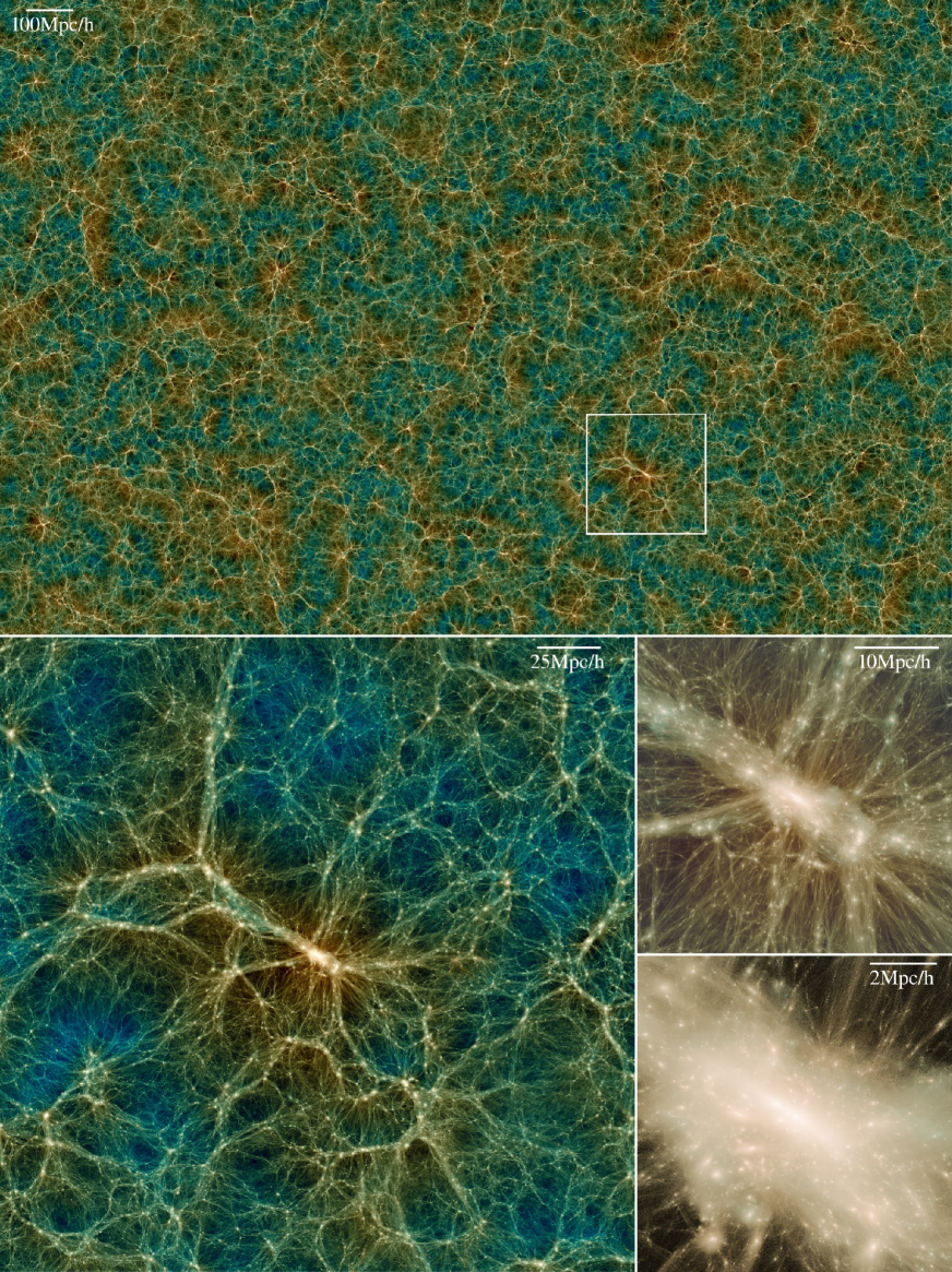
Figure 1: Dark matter distribution of the Uchuu simulation at $z=0$. The top panel shows a 2000 $\,h^{-1}\rm Mpc$ $\times$ 1333 $\,h^{-1}\rm Mpc$ slice of thickness of 25 $\,h^{-1}\rm Mpc$. The three bottom panels zoom in on largest halo in Uchuu, on scales of 250, 38, and 9.4 $\,h^{-1}\rm Mpc$ (moving clockwise). The white box in the top panel is the same region visualized in the left-bottom panel, equivalent in scale to the Bolshoi simulation (Klypin et al., 2011). The evolution of the largest halo is visualized in Figure 3.

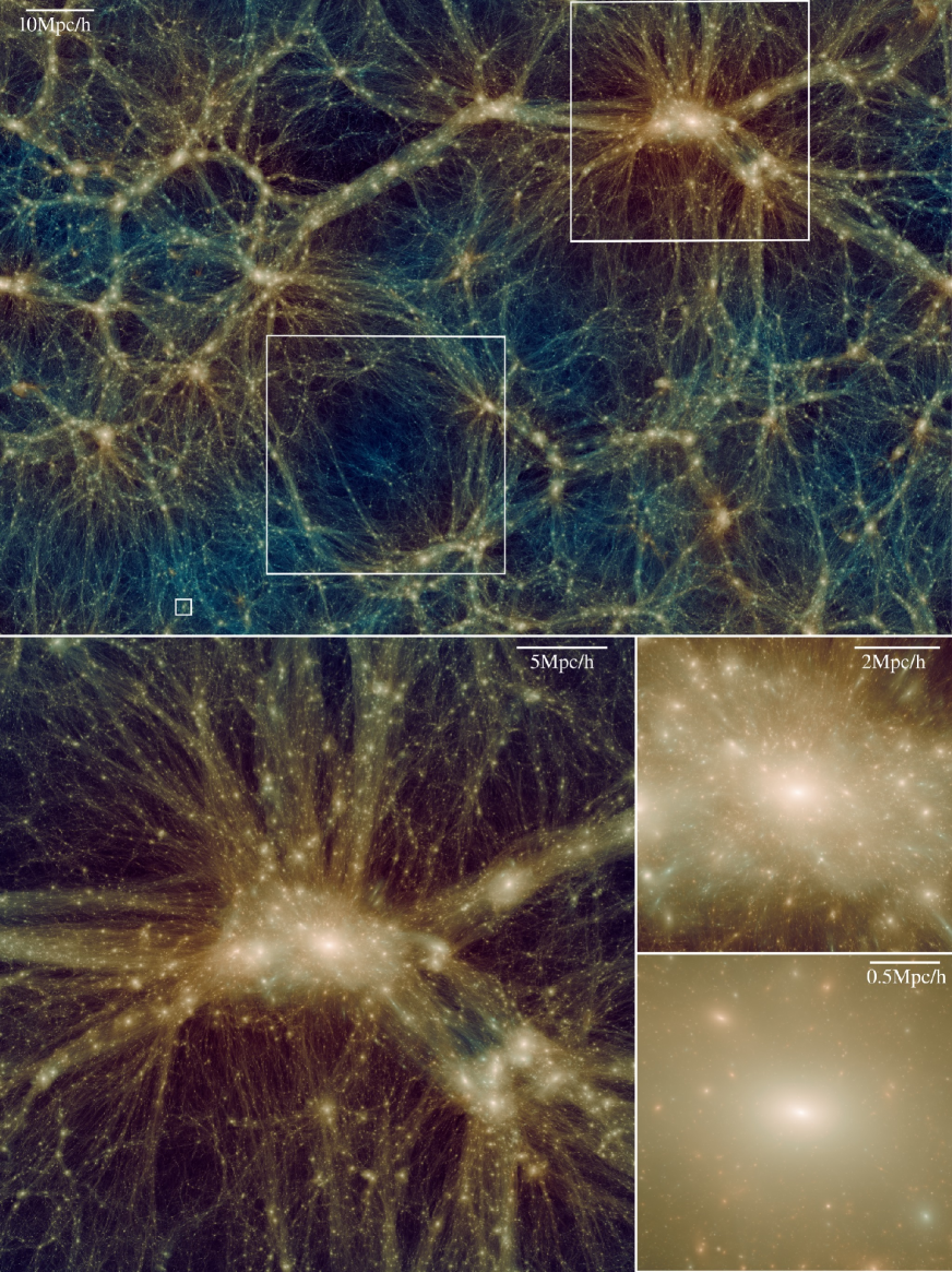
Figure 2: Dark matter distribution of the higher resolution Shin-Uchuu simulation at $z=0$. The top panel shows a 140 $\,h^{-1}\rm Mpc$ $\times$ 93 $\,h^{-1}\rm Mpc$ slice of thickness of 17.5 $\,h^{-1}\rm Mpc$. The three bottom panels zoom in on the largest halo in Shin-Uchuu, on scales of 35, 7.5, and 2.3 $\,h^{-1}\rm Mpc$ (moving clockwise). The upper-most white box in the top panel is the same region visualized in the left-bottom panel. The middle white box is a void region selected by eye, while the lower-most white box is a Milky-way sized halo. The evolutionary paths of the latter two regions are visualized in Figure 3.

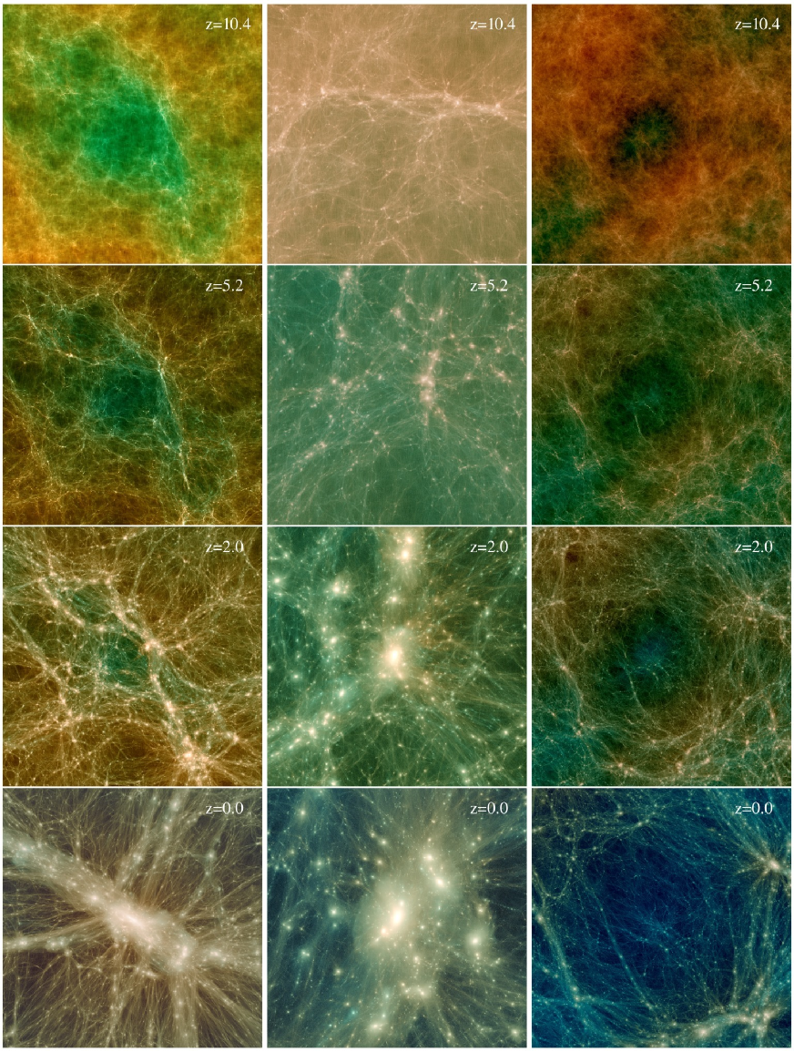
Figure 3: Evolution of three different environments drawn from the Uchuu simulation suite. Redshift is marked in each panel, $z=10.4$, 5.2, 2.0, and 0.0, from top to bottom. The three environments are: left, the largest halo in the Uchuu simulation; middle, a Milky Way sized halo in the Shin-Uchuu simulation; and right, a void selected by eye in the Shin-Uchuu simulation. The side lengths shown are 38, 2.3, and 35 $\,h^{-1}\rm Mpc$ for the left, middle, and right panels, respectively.

To generate the initial conditions for each simulation, we used the parallel 2LPTic code adopting second-order Lagrangian perturbation theory (Crocce et al., 2006). We calculated the matter transfer function using the online version of Camb (Lewis et al., 2000). Throughout, the latest cosmological parameters measured by the Planck Satellite (Planck Collaboration et al., 2020) were adopted: $\Omega_{0}=0.3089$, $\Omega_{\rm b}=0.0486$, $\lambda_{0}=0.6911$, $h=0.6774$, $n_{\rm s}=0.9667$, and $\sigma_{8}=0.8159$. The initial redshift for all simulations was 127. The gravitational evolution of each dark matter particle was calculated using the massively parallel TreePM code, GreeM (Ishiyama et al., 2009; Ishiyama et al., 2012). This was run on the Aterui II supercomputer at the Center for Computational Astrophysics (CfCA), National Astronomical Observatory of Japan, and the K computer at the RIKEN Advanced Institute for Computational Science. The evaluation of the tree forces was accelerated by the Phantom-grape software (Nitadori et al., 2006; Tanikawa et al., 2012, 2013; Yoshikawa & Tanikawa, 2018). 50 particle snapshots covering $z=14$ to 0 were written to disk.

To identify bound structures within the particle data at each snapshot, the rockstar phase space halo/subhalo finder (Behroozi et al., 2013a) was run. We then constructed merger trees using the consistent trees code (Behroozi et al., 2013b). However, by default, consistent trees does not run in parallel in a distributed memory environment. Hence, our use of consistent trees needed to be modified to make merger tree construction possible on simulations of the size of those in the Uchuu suite.

To overcome this hurdle, we split the full box of each simulation into smaller regularly spaced sub-volumes, and ran consistent trees for each sub-volume separately. In the case of the Uchuu simulation, the rockstar catalogues for each snapshot were broken into $20^{3}$ sub-catalogues of comoving volume $2000^{3}/20^{3}=100^{3}$ $(h^{-1}\rm Mpc)^{3}$. These sub-catalogues were then grouped across redshift to construct the merger trees, where sub-catalogues in each group occupy the same Euler comoving volume. However, halos and subhalos can have progenitor/descendant relationships that lie outside of such defined groups. To account for this, we added halos and subhalos to the group if they lay within a 25 $\,h^{-1}\rm Mpc$ distance from any edge of the corresponding Euler volume of the group. However, this also meant that added halos and subhalos could be duplicated in multiple groups, and after running consistent trees across all groups, multiple merger tree files constructed separately could have the same trees that contain these overlapping halos and subhalos. To correct for this, we ran a final step to clean such overlapping trees from all tree files except for one, thus removing any duplicates. In this way the merger trees are consistently and efficiently constructed for the entire box. To show the robustness of this method, in Appendix D we compare merger trees from the mini-Uchuu simulation constructed by this method and the original consistent trees code.

In addition to the Uchuu and Shin-Uchuu simulations, we use an additional small volume but ultra-high resolution simulation, Phi-4096, described in Table 1, focused on $z>7.5$. This simulation extends the halo mass range down to $10^{7}$$\rm M_{\odot}$ at high redshift and helps with the evaluation of resolution effects. Phi-4096 is also used when we later examine the halo mass-concentration relation. The cosmological parameters of Phi-4096 are slightly different from those of the Uchuu suite: 1.6 per cent larger for $\sigma_{8}$ and less than 1 per cent for the remaining parameters. Dutton & Macciò (2014) show that the average concentration of a halo increases by about 8 per cent when $\sigma_{8}$ increases by 7.9 per cent. The latter is much larger than the difference between the Uchuu and the Phi-4096 simulations, and thus we treat all simulations equally in what follows. The initial conditions of Phi-4096 were generated by the publicly available code, music (Hahn & Abel, 2011). All other numerical tools used to process and study Phi-4096 were the same as those for the Uchuu simulations.

Figure 1 shows dark matter distribution of the Uchuu simulation at $z=0$. The top panel shows a 2000 $\,h^{-1}\rm Mpc$ $\times$ 1333 $\,h^{-1}\rm Mpc$ slice of thickness of 25 $\,h^{-1}\rm Mpc$. To calculate density fields, we used the tetrahedron quadrupole particle mesh (T4PM) method (Hahn et al., 2013). Vast cosmic web structures are clearly visible. The three bottom panels are close-ups of the largest halo in the box at different zoom levels, highlighting the detail Uchuu can resolve. The mass of this halo is $\sim 5.0\times 10^{15}$$\,h^{-1}\rm M_{\odot}$. More than a thousand halos with mass greater than $\sim 1.0\times 10^{15}$$\,h^{-1}\rm M_{\odot}$ exist in Uchuu, which allows us to study such rare objects with unprecedented statistics. Each such halo is resolved by more than three million particles.

Figure 2 shows dark matter distribution of the Shin-Uchuu simulation at $z=0$. The top panel shows a 140 $\,h^{-1}\rm Mpc$ $\times$ 93 $\,h^{-1}\rm Mpc$ slice of thickness of 17.5 $\,h^{-1}\rm Mpc$. The format is the same as in Figure 1, where we again zoom in on the largest structure in the box. Figure 3 shows the evolution of three selected regions at redshifts $z=10.4$, 5.2, 2.0, and 0.0: the largest cluster halo in the Uchuu simulation, a Milky Way sized halo in the Shin-Uchuu simulation, and a void selected by eye in the Shin-Uchuu simulation. The evolution of the cosmic web leading to protocluster formation is clearly visible in the left row. In the center row, thanks to the high resolution of the Shin-Uchuu simulation we observe many progenitor halos of the Milky-Way system, even at $z>10$. More than ten thousand of Milky-Way sized halos are formed in Shin-Uchuu, which enables us to study the statistics of such halos with unprecedented resolution. In the right row, which tracks the evolution of a large cosmic void, we see how small halos form even within such an underdense environment, highlighting both the large spatial volume and the high resolution of Shin-Uchuu.

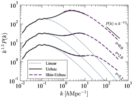
Figure 4: Power spectra of the Uchuu (solid curves) and Shin-Uchuu (dashed curves) simulations. Results are shown for $z=0.0,2.0$, and 5.2 (top to bottom), where each are multiplied by $k^{1.5}$ to more clearly highlight the BAO features. The dotted curves show the linear power spectra. At high-$k$, the power is close to $P(k)\propto k^{-2.5}$.

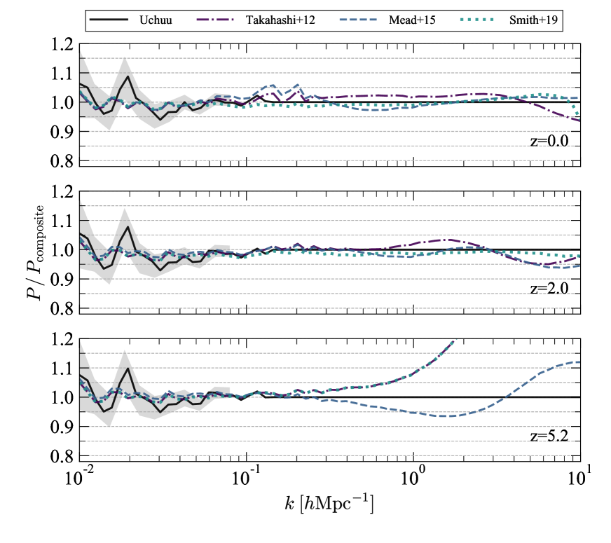
Figure 5: Comparison of power spectra at low-$k$ with predictions from three models of the non-linear matter power spectrum (Takahashi et al., 2012; Mead et al., 2015; Smith & Angulo, 2019). The top, middle, and bottom panels show the results for $z=0.0,2.0$, and $5.2$, respectively. The reference spectra, $P_{\rm composite}$, are taken from the Uchuu simulation for $k>0.1$ $\,h\,\rm Mpc^{-1}$ and an ensemble of glam simulations (Klypin & Prada, 2018) for $k<0.1$ $\,h\,\rm Mpc^{-1}$. The grey shaded regions are the estimated $1\sigma$ scatter of the Uchuu simulation.

3 Results

We first present the basic properties of halos, matter power spectra, and mass functions of the Uchuu simulations. Then we propose an accurate model of halo concentrations that describes our simulations.

3.1 Power spectrum

Large number of particles and high force resolution of Uchuu simulations allow us to measure the power spectrum of dark matter fluctuations for a very large range of wavenumbers. However, in order to use this potential advantage, we need to implement a technique that is different from traditionally used method based on a large single mesh. We start with a single mesh of size $N_{\rm g}=2400$ in one dimension. The mesh covers the whole computational box $L$. The Cloud-In-Cell technique is applied to all particles $N_{\rm p}$ to find the dark matter density on this mesh. In this process the "weight" of each particle is assumed to be $W_{1}=N_{\rm g}^{3}/N_{\rm p}$. In this case the total "weight" of all particles is simply the total number of grid points. Using the FFT we find the power spectrum of the density field. Because the mesh is not very large, it lacks information on wavenumbers larger than the Nyquist frequency $k_{\rm Ny}=(\pi/L)N_{\rm g}$ of the mesh.

On the next step we again use the $N_{\rm g}^{3}$ mesh, but this time it covers only half of the computational box, and, thus, it has box size $L/2$, and its Nyquist frequency is twice larger. When estimating the density, the coordinates of each particle are folded with the new box size: $\tilde{x}=\mod(x,L/2)$ and the same is applied for $y-$ and $z-$coordinates. The density assignment is made using the new coordinates $(\tilde{x},\tilde{y},\tilde{z})$ and the particle weight is increased by factor $2^{3/2}$. Again, we use the FFT to find the power spectrum. This time it does not have any information about waves longer than $L/2$, but it has information on frequencies that are twice higher than on the first step. We proceed with new levels each time reducing twice the box size, increasing twice the mesh Nyquist frequency and increasing particle "weight" by $2^{3/2}$. In total we have six levels of meshes with the combined range of wavenumbers from $(2\pi/L)$ to $2^{5}N_{\rm g}(2\pi/L)$.

The final power spectrum of the whole simulation is constructed from the set of six power spectra obtained for each mesh. We start with the first power spectrum corresponding to the box $L$. The power spectrum is corrected for the aliasing. All estimates are taken until we reach the points where the aliasing correction falls below $0.85$. At this moment we proceed to the results of the next mesh with twice smaller box size. The process continues for all six levels of meshes.

Figure 4 shows the evolution of the power spectra of dark matter from the Uchuu and Shin-Uchuu simulations. The Uchuu suite allows us to plot a large range of wave numbers covering five orders of magnitude. At low-$k$, the simulation follows the linear matter power spectrum. Power spectra are multiplied by $k^{1.5}$, where $k$ is the wave number, which clearly highlights the Baryon Acoustic Oscillations (BAO) features, including the first and second peaks at $k\sim 0.07$ and 0.13 $\,h\,\rm Mpc^{-1}$ for $z<2$. Other small peaks can be seen at $z>2$, but these are gradually smeared out at lower redshift as the spectra is influenced by non-linear structure growth. Both simulations agree well with each other in the overlapping region, $1<k<10$ $\,h\,\rm Mpc^{-1}$. The agreement is similar to that found by Schneider et al. (2016), who compared power spectra calculated by three different $N$-body methods and showed convergence at the one percent level for $k<1$ $\,h\,\rm Mpc^{-1}$, and three percent level for $k<10$ $\,h\,\rm Mpc^{-1}$when using standard run parameters. In their tests, gadget-3 (Springel, 2005) was adopted, and its time-stepping method and choice of run parameters are similar to what was used in the Uchuu and the Shin-Uchuu simulations.

Figure 5 shows a comparison between the Uchuu matter power spectra at low to middle-$k$ with predictions from three models of nonlinear structure evolution (Takahashi et al., 2012; Mead et al., 2015; Smith & Angulo, 2019). The spectra of Mead et al. (2015) are calculated using hmcode, and of Takahashi et al. (2012) and Smith & Angulo (2019) using ngenhalofit. We construct the reference spectra $P_{\rm composite}$ as a composite of the Uchuu power spectrum for $k>0.1$ $\,h\,\rm Mpc^{-1}$, and an average of an ensemble of 17 glam Particle-Mesh simulations (Klypin & Prada, 2018) for $k<0.1$ $\,h\,\rm Mpc^{-1}$ to ameliorate the effects of cosmic variance. The glam simulations were run in $2h^{-1}{\rm Gpc}$ side-length boxes with $2000^{3}$ particles moving in a $7000^{3}$ mesh, providing $8.6\times 10^{10}$$\,h^{-1}\rm M_{\odot}$ mass per particle resolution.

The shaded regions in Figure 5 show the estimated $1\sigma$ scatter of the Uchuu simulation, which overlaps with the composite power spectra, meaning that deviations of the simulation spectra at $k<0.1$ $\,h\,\rm Mpc^{-1}$ are due to the cosmic variance. For $k>0.1$ $\,h\,\rm Mpc^{-1}$, the model prediction of Smith & Angulo (2019) agrees remarkably well with the Uchuu simulation at $z=0$ and $z=2$, where the error is within $\sim$ 2 per cent up to $k=10$ $\,h\,\rm Mpc^{-1}$. As expected, this model fails to predict the spectra at $z=5.2$ because it is not calibrated beyond $z=3$ and reverts to that provided by Takahashi et al. (2012). The models of Takahashi et al. (2012) and Mead et al. (2015) predict the power within $\sim$ 5 per cent at $z=0.0$ and $2.0$. At $z=5.2$, Mead et al. (2015) predicts the power within $\sim$ 5 per cent at $k<4$ $\,h\,\rm Mpc^{-1}$, which is better than the others, even though it is not calibrated for such high redshifts. In general, the accuracy at high redshift reflects how the underlying models are constructed.

These results demonstrate that our simulations are accurate across a wide dynamic range, from BAO to very small scales, reinforcing their usefulness for a wide range of applications.

3.2 Halo mass function

Figure 6 shows the halo mass function multiplied by $M_{\rm vir}^{2}$ and divided by the mean cosmic density for the Uchuu and the Shin-Uchuu simulations at $z=0$, $2.0$, and $5.2$, where $M_{\rm vir}$ is the halo virial mass. We only consider halos with more than 40 particles, corresponding to a minimum mass of $1.3\times 10^{10}$$\,h^{-1}\rm M_{\odot}$ for Uchuu and $3.6\times 10^{7}$$\,h^{-1}\rm M_{\odot}$ for Shin-Uchuu. With this lower limit, the combined mass range spans approximately eight orders of magnitude, reflecting the power of our very large simulation set. The convergence between both simulations is remarkably good, within a few per cent.

Figure 6 also considers the halo mass fitting function proposed by Despali et al. (2016), shown by each solid line. The fractional difference between this function and each simulation is presented in Figure 7 for Uchuu (filled circles) and Shin-Uchuu (filled squares). This comparison highlights a 5 per cent difference at $z=0$ over a broad range of halo mass up to $M_{\rm vir}<\sim 3\times 10^{14}$$\,h^{-1}\rm M_{\odot}$. Despali et al. (2016) present different parameterisations of their fitting function specifically for halos more massive than $M_{\rm vir}>3\times 10^{13}$$\,h^{-1}\rm M_{\odot}$ (shown in their Table 3). These provide a better fit in our analysis for Uchuu halos of mass $M_{\rm vir}>2\times 10^{14}$$\,h^{-1}\rm M_{\odot}$. Overall, we find a difference of less than 10 per cent for halos with $M_{\rm vir}<10^{15}$$\,h^{-1}\rm M_{\odot}$. At $z=2.0$ and $5.2$, this difference increases to around 10 per cent. At the massive end of the mass function, the fitting function underestimates the number of massive halos, while it overestimates the number of less massive halos. We expect this is related to challenges of cosmic variance and the accuracy of the simulations used to derive the fitting function (see also Knebe et al. (2013)).

We do not perform an extensive analysis of the mass function in this paper, but leave it for a dedicated study at a later time.

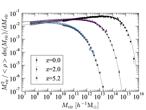
Figure 6: Mass function of distinct halos multiplied by $M_{\rm vir}^{2}$ and divided by the mean cosmic density from the Uchuu (filled symbols) and the Shin-Uchuu (open symbols) simulations at $z=0.0$, $2.0$ and $5.2$. These cover approximately eight orders of magnitude in halo mass. The error bars correspond to Poisson error. We only consider halos with more than 40 particles. Solid curves show the fitting functions proposed by Despali et al. (2016).

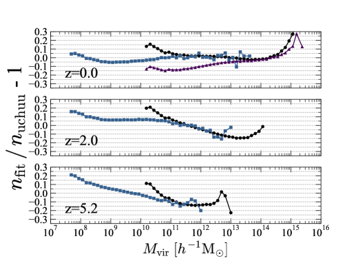
Figure 7: Comparisons of the halo mass functions of Uchuu (filled circles) and Shin-Uchuu (filled squares) with the fitting functions proposed by Despali et al. (2016). Triangles at $z=0$ compare against the specific high mass halo fitting function of (Despali et al., 2016), as described in the text.

3.3 Subhalo mass function

In Figure 8 we display the mean subhalo mass function for the Uchuu simulation at $z=0$, $N(>M_{\rm acc}/M_{\rm vir})$, computed in four narrow (5 per cent) bins of host halo mass, $M_{\rm vir}=10^{15},10^{14},10^{13},10^{12}$$\,h^{-1}\rm M_{\odot}$, where the subhalo mass $M_{\rm acc}$ is defined at the time of first accretion. Solid lines with different colors correspond to different host halo mass bins as label in the figure panel. Overall our results are in good agreement with previous simulation works and model predictions (e.g., Rodríguez-Puebla et al., 2016; Hiroshima et al., 2018; van den Bosch et al., 2018; van den Bosch & Ogiya, 2018, and references therein) that explore the subhalo mass function shape and host halo mass dependence. This figure also shows the best-fitted Schechter-like function (dotted line) to the Bolshoi Planck / MultiDark Planck subhalo mass function of host halo mass $M_{\rm vir}=10^{15}$$\,h^{-1}\rm M_{\odot}$ (see Rodríguez-Puebla et al., 2016). We highlight the remarkable agreement of the slope at the low-mass end, equal to -0.75, in agreement with previously reported works. Yet, the results obtained from Uchuu reveal a clear difference in the shape at the exponential tail, thanks to our superb statistics, with a shallow decline towards higher $M_{\rm acc}/M_{\rm vir}$ values. The $\sim 20$ per cent difference in normalisation is due to the difference in the adopted cosmological parameters among both simulation suites. A detailed study and interpretation of these results will be presented in a forthcoming paper (Moliné et al., in preparation).

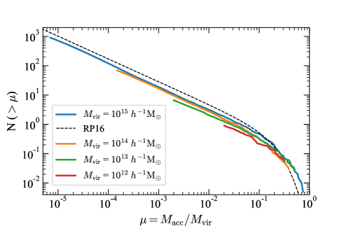
Figure 8: The Uchuu subhalo mass function at $z=0$, $N(>\mu$), for different host halos as a function of $\mu=M_{\rm acc}/M_{\rm vir}$ (solid curves). As a reference, the dashed line shows the best-fitted Schechter-like function fit to the Bolshoi Planck / MultiDark Planck simulations (Rodríguez-Puebla et al., 2016). Note the similar overall power-law slope but different shape at the exponential tail due to the much higher statistics of Uchuu.

3.4 Mass-concentration relation: all halos

The mass-concentration relation is an essential diagnostic to characterise the internal structure of halos. Many past studies have investigated the dependence of concentration on halo mass and redshift (e.g., Prada et al., 2012; Ludlow et al., 2012; Dutton & Macciò, 2014; Correa et al., 2015; Klypin et al., 2016; Okoli & Afshordi, 2016; Pilipenko et al., 2017; Child et al., 2018; Diemer & Joyce, 2019; Ishiyama & Ando, 2020). These works show that halo concentration increases with decreasing halo mass and redshift, with the exception of the most massive and rare halos for which the concentration may increase with increasing mass (e.g., Prada et al., 2012; Klypin et al., 2016; Diemer & Joyce, 2019). Halo concentration also depends on the background cosmology and the relaxation state of halos (e.g., Dutton & Macciò, 2014; Klypin et al., 2016), with relaxed halos exhibiting slightly larger concentrations.

In this paper, we extend these past works thanks to the statistical power of the Uchuu simulation suite, which covers an unprecedented range in halo mass at high resolution. For halos with an NFW profile (Navarro et al., 1997), concentration is defined as the ratio of the halo radius to the characteristic radius $r_{\rm s}$ of the NFW profile. In general, there are different ways to define the halo radius and mass. Here we use two methods, with halos defined either by the radius $r_{\rm 200}$ where the average spherical overdensity is 200 times the critical density, or by the virial overdensity that slightly evolves with the redshift. We will label quantities related to each of the definitions by the indexes "200" or "vir", respectively. Unless otherwise noted, our main results are show with $r_{\rm 200}$. An alternative definition, using $r_{500}$, is often used for galaxy cluster modeling, in which the average spherical overdensity is 500 times the critical density.

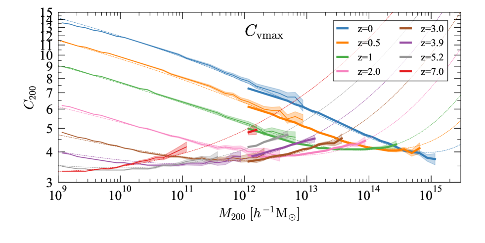
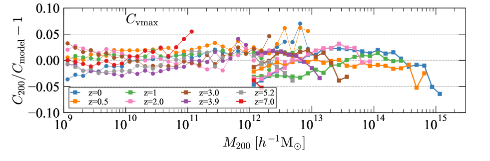
Figure 9: Top panel: Mass-concentration relation of halos for the Uchuu (thick curves) and the Shin-Uchuu (thin curves) simulations. Median values with statistical uncertainties in each mass bin are shown. The concentrations are estimated using $V_{\rm max}$ given by eq.(1). The dashed curves are predictions of the analytical model described by eq. (2) in Appendix B. Bottom panel: The fractional difference between the halo concentrations of the Uchuu (squares) and the Shin-Uchuu (circles) simulations and the model predictions. It illustrates that the analytical model provides an accurate fit to the actual concentrations with an error less $\sim 5$ per cent, for the redshift range $0<z<7$ and halo masses covering six orders-of-magnitude.

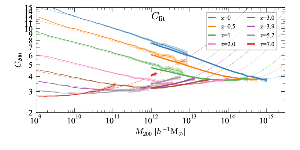
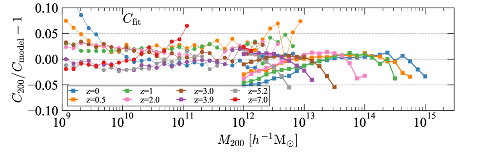
Figure 10: The same as in Figure 9 but for concentrations estimated by profile fitting. The plot shows that the main tendencies of the concentration-mass relation do not depend on the method used to find the concentration. This includes the upturn in concentration found at large masses.

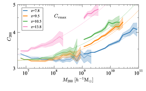
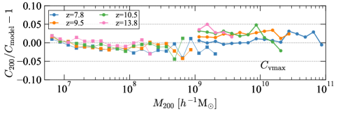
Figure 11: Halo concentrations at very large redshifts and small masses. Top panel: Mass-concentration relation for the Shin-Uchuu (thick curves) and the Phi-4096 (thin curves) simulations. In both cases, concentrations are estimated using the $V_{\rm max}$ method. Median values with statistical uncertainty in each mass bin are shown. The dashed curves provide the model prediction described by eq. (2). Bottom panel: The fractional difference between the halo concentrations of the Shin-Uchuu (circles) and the Phi-4096 (squares) simulations and the analytical model. Again, we find the model fits the simulation with an accuracy of better than $\sim 5$ per cent across a large redshift and mass range.

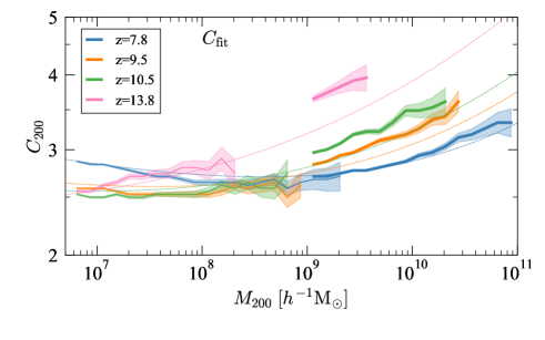
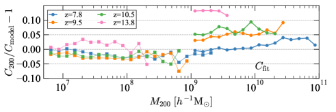
Figure 12: The same as in Figure 11, but for concentrations estimated by profile fitting.

For halos well fit by an NFW profile, two parameters – mass and concentration – uniquely define the density distribution. The situation is more complicated for halos that do not follow an NFW profile. Indeed, some halos (and especially very massive and rare ones) are better described by the Einasto profile (Navarro et al., 2004; Dutton & Macciò, 2014; Klypin et al., 2016). In this case one needs three parameters. If we still choose to use only two – mass and concentration – how do we then define the concentration? One must be careful when taking the naive association of the core radius as the radius $r_{-2}$ where the log-log slope of the density profile is -2, which is valid for the NFW profile. In this case two halos with obviously different concentrations may have the same $r_{-2}$ because they have different shape parameters of the Einasto profile. Indeed, Klypin et al. (2016) present examples that this typically happens with massive halos. We similarly show cases of halo profiles of this kind in Appendix A. Keeping the above caveats in mind, for consistency in our analysis we use the same definition of concentration and the same algorithm as in the case of the two-parameter NFW profile. For such halos the accuracy of the prediction of their density distribution is reduced. However, in practice the errors for such halos are relatively small, even in extreme cases. For example, the density profile errors are less than 5 per cent for the most massive halos at $z=0$ at radii larger than 0.01 of the halo radius.

Halo concentration also depends on the dynamical state of the halo, with relaxed halos tending to have larger concentrations (e.g., Prada et al., 2012; Ludlow et al., 2012; Klypin et al., 2016). The selection criteria for relaxed halos can differ in literature, and can introduce systematic biases. For example, Prada et al. (2012) found an upturn in the concentrations of massive halos in both their "all" and "relaxed" samples, while Ludlow et al. (2012) did not find such an upturn in their relaxed ones. In this section we use all halos regardless of their relaxation state. Relaxed halos and the upturn are discussed in the next section.

There are different methods that can be applied to the particle data to estimate halo concentration. One can construct and then fit the density profile in spherical shells. In this case the results can be affected by the quality of the fit and by the chosen binning algorithm. Alternatively, we can define the concentration by numerically solving the following equations (Klypin et al., 2011; Prada et al., 2012):

$$V_{200}=\left(\frac{GM_{200}}{R_{200}}\right)^{1/2},\quad\frac{V_{\rm max}}{V_{200}}=\left(\frac{0.216c}{f(c)}\right)^{1/2},$$ (1)

where $f(c)=\ln(1+c)-c/(1+c)$ and $V_{\rm max}$ is the maximum circular velocity. In this paper we use different notations to indicate these different methods. Concentrations obtained by fitting density profiles are labeled as $c_{\rm fit}$ while the concentrations from the $V_{\rm max}$ method are denoted as $c_{\rm vmax}$. If no explicit label is given, the concentration was obtained with the $V_{\rm max}$ method.

Appendix A presents estimates of the errors for different methods and the dependencies of the estimates on numerical effects such as the number of particles and force resolution. There is a general trend that follows from the nature of the methods. The $V_{\rm max}$ is sensitive to the mass distribution in the relatively peripheral region of a halo and it is not sensitive to the mass distribution at the center or to any local fluctuations. This is a good method, if one is interested in the main body of the halo, but not its center. The density fitting method is more sensitive to the central regions. However, it is also prone to errors produced by non-relaxed features.

Both definitions produce similar values at lower redshifts, $z<1$, where halos tend to be more relaxed. On average, the differences in concentration are less than few per cent. However, when the fraction of non-relaxed halos increases (either at high redshifts or at the high-mass end) $c_{\rm fit}$ results in smaller concentrations (Dutton & Macciò, 2014). At $z=5$, the difference between the two estimates can reach up to 15 per cent. See Appendix A for more details.

When fitting our results with different analytical models we find that the model proposed by Diemer & Joyce (2019) (with modifications) is the most accurate. However, their original calibration gave large errors that were $\sim 10$ per cent at low redshifts and $\sim 20$ per cent at high redshifts for concentrations from the $V_{\rm max}$ method. After tuning the parameters using Uchuu data covering large range of redshifts and masses, the final model showed significant improvements, even for concentrations based on $V_{\rm max}$. Following Diemer & Joyce (2019), we assume that the halo concentration has the following functional form:

$$c=C\left(\alpha_{\mathrm{eff}}\right)\times\tilde{G}\left(\frac{A\left(\alpha_{\mathrm{eff}}\right)}{\nu}\left[1+\frac{\nu^{2}}{B\left(\alpha_{\mathrm{eff}}\right)}\right]\right),$$ (2)

where $\nu=\delta_{\rm c}/\sigma(M)$ is the height of the density peak, $\delta_{\rm c}=1.686$ is the critical overdensity for spherical collapse, and $\sigma(M)$ is the rms density fluctuation. Factor $n_{\rm eff}$ is the effective slope of the $\sigma(M)$ function, and $\alpha_{\rm eff}$ is the linear growth rate of fluctuations. Parameters $A$, $C$ and $B$ depend on $n_{\rm eff}$. The function $\tilde{G}$ depends on the assumed density profile (here NFW). Appendix B gives details of the approximation. Equation 2 has six free parameters, which we find by minimizing the errors using our Uchuu suite of simulations. Table 2 presents our parameters for the analytical model. We also present the parameters for concentrations $c_{\rm vir}$ estimated using the $V_{\rm max}$ method and profile fitting.

Figure 9 (top panel) shows the mass-concentration relation of the Uchuu and Shin-Uchuu simulations and their redshift evolution. Median values with statistical uncertainty in each mass bin are shown. The concentrations are estimated using the $V_{\rm max}$ method (eq.(1)). At low redshift, the relation follows a well-known power law behaviour except at the highest masses. We observe a flattening and an upturn with increasing mass, consistent with previous findings (e.g., Prada et al., 2012). This flattening and upturn gradually shifts to lower mass at higher redshift. The Shin-Uchuu simulation produces slightly larger concentrations than Uchuu in the overlap region ($10^{12}\sim 10^{13}$$\,h^{-1}\rm M_{\odot}$) at $z<3$. However, both simulations follow the same trend. Figure 10 (top panel) also shows the mass-concentration relation, but where concentrations are estimated by the profile fitting method. Together, Figures 9 and 10 highlight that the main tendencies of the concentration-mass relation does not depend on the method to find concentration in our simulation suite. This includes the upturn in the concentration at large masses.

With the unprecedented high resolution and statistical power of the Shin-Uchuu and the Phi-4096 simulations, we can statistically study the mass-concentration relation at mass $M_{200}<10^{11}$$\,h^{-1}\rm M_{\odot}$ and redshift $z>7$ for the first time. The top panels of Figures 11 and 12 show the mass-concentration relation of the Shin-Uchuu and Phi-4096 simulations and their redshift evolution, using the $V_{\rm max}$ and profile fitting methods, respectively. For both, concentration increases with increasing mass, opposite to the behavior see at lower redshift. This should be compared to the flattening and upturn identified in Figures 9 and 10. Again, the main trends of the concentration-mass relations do not depend on the method to find concentration.

The bottom panel of both Figures 9 and 11 show residuals of the concentration estimated using the $V_{\rm max}$ method relative to the model. Across most of the halo mass and redshift range the difference is within 5 per cent, although there are a few exceptions. This highlights that the accuracy provided by the model is quite good for masses spanning nearly eight orders of magnitude. Similarly, the bottom panel of both Figures 10 and 12 show residuals using the profile fitting method. The model accuracy here is also good but slightly worse than for concentrations estimated using $V_{\rm max}$. Again, the difference is within 5 per cent for most halo masses and redshifts, although it can increase to nearly 10 per cent in places. This is prominent for rare objects at high redshift.

We also explore the concentration relation using $r_{500}$: $\rm c_{500}=r_{500}/r_{s}$. The same fitting procedure described in this Section is used to find the best fitting parameters of the mass-concentration relation. Plots for concentration-mass relation are presented in Figure 21. We present concentration estimated using only the profile fitting because it is better to describe the halo inner profile than the $V_{\rm max}$ method as shown in Appendix A. We use only data at $z\leq 7$ to ensure the fitting error within 5 per cent. Including data at $z>7$, the fitting error increases from 5 to 10 per cent.

Table 2 presents the parameters for the $c_{200}$, $c_{\rm vir}$ and $c_{500}$ halo definitions estimated using the $V_{\rm max}$ and profile fitting methods. In general, the model accuracy is very similar for $c_{200}$; the difference is within 5 per cent for most halo masses and redshifts, but is close to 10 per cent for rare objects at high redshift when concentrations are estimated by profile fitting.

Table 2: Best fitting parameters of the mass-concentration relation for the model eq. (2). Parameters are given for different methods of finding concentrations, for different halo selections, and for different halo definitions. We present concentration $c_{500}$ estimated using only the profile fitting because it is better to describe the halo inner profile than the $V_{\rm max}$ method as shown in Appendix A.

$c$	$\kappa$	$a_{0}$	$a_{1}$	$b_{0}$	$b_{1}$	$c_{\alpha}$
Vmax   All halos
$c_{200}$	1.10	2.30	1.64	1.72	3.60	0.32
$c_{\rm vir}$	0.76	2.34	1.82	1.83	3.52	$-0.18$
Fit   All halos
$c_{200}$	1.19	2.54	1.33	4.04	1.21	0.22
$c_{\rm vir}$	1.64	2.67	1.23	3.92	1.30	$-0.19$
$c_{500}$	1.83	1.95	1.17	3.57	0.91	0.26
Vmax   Relaxed halos
$c_{200}$	1.79	2.15	2.06	0.88	9.24	0.51
$c_{\rm vir}$	2.40	2.27	1.80	0.56	13.24	0.079
Fit   Relaxed halos
$c_{200}$	0.60	2.14	2.63	1.69	6.36	0.37
$c_{\rm vir}$	1.22	2.52	1.87	2.13	4.19	$-0.017$
$c_{500}$	0.38	1.44	3.41	2.86	2.99	0.42

In spite of the fact that we use the same functional form proposed by Diemer & Joyce (2019), our parameters of the approximation are quite different from theirs. Figure 13 compares predictions for such concentrations. The agreement between the predictions is remarkably good for $c_{\rm fit}$ estimates at $z=0$ with just $\sim 2$ per cent differences for masses $M<5\times 10^{14}$$\,h^{-1}\rm M_{\odot}$. The differences increase at high redshifts and become $\sim 20$ per cent at $z=10$. This is a good improvement as compared with the situation just a few years ago. For example, disagreement between Correa et al. (2015) and Diemer & Kravtsov (2015) was 20 per cent at $z=0$, $M=2\times 10^{14}$$\,h^{-1}\rm M_{\odot}$. A more detailed comparison of results provided by different publications can be found in Diemer & Joyce (2019).

3.5 Mass-concentration relation: relaxed halos

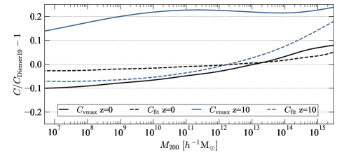
Figure 13: Comparison of the predictions of halo concentrations $c_{200}$ in this paper with those of Diemer & Joyce (2019). Both predictions use the same functional form, but different parameters.

So far we have presented mass-concentration relations for all halos regardless of their dynamical state. For some studies one may need to remove rare transient events (e.g., due to ongoing major mergers) and to study more relaxed halos (e.g., Neto et al., 2007; Prada et al., 2012; Ludlow et al., 2012; Klypin et al., 2016). There are no clear selection criteria of relaxed halos.

The first obvious choice is the virial parameter $2K/|W|-1$, where $W$ and $K$ are the potential and kinetic energies, respectively. The virial parameter should be equal to zero for objects in virial equilibrium. As such, this parameter has been extensively used in the past (e.g., Neto et al., 2007; Ludlow et al., 2012). However, many results show that otherwise relaxed halos can have systematically too large a $2K/|W|-1$, as if the kinetic energy is too big for a given potential energy. The problem is extreme with values $2K/|W|-1>0.3$ being typical for halos at redshifts $z>3$ (Davis et al., 2011; Klypin et al., 2016). If this were true, halos would have dissolved or collapsed on a dynamical time-scale. Analysis of individual and average halo profiles do not show any signs of catastrophic collapse or expansion: inner halo regions have zero average radial velocities while there are small infalling velocities close to the virial radius. This failure of the virial parameter is attributed to simplistic treatment of the virial theorem. Dark matter halos are not isolated objects. When applying the virial theorem, one must include the surface pressure term, which, for spherical halos, is $S_{\rm p}=4\pi R^{3}_{\rm vir}\rho_{\rm vir}v_{\rm r}^{2}$, where $v_{\rm r}^{2}$ is the dispersion of the radial velocity. Once this correction is applied, the virial parameter becomes significantly smaller (Shaw et al., 2006; Davis et al., 2011; Klypin et al., 2016). Furthermore, large and complicated corrections and uncertainties due to non-spherical halo shapes make the virial parameter much less useful as an indicator of non-equilibrium halos. This is why the virial parameter is currently either not utilized, or used with a very large upper limit (Correa et al., 2015; Klypin et al., 2016; Child et al., 2018).

There are other conditions for selecting relaxed halos. These include the fraction of mass in subhalos $f_{\rm sub}$, the offset parameter $X_{\rm off}$, and the spin parameter $\lambda$. We define the offset parameter as the distance between the center of halos and center of mass: $X_{\rm off}=|\vec{r}_{\rm center}-\vec{r}_{\rm cm}|/R_{\rm vir}$. The spin parameter is defined as $\lambda=J|E|^{1/2}/GM^{5/2}_{\rm vir}$, where $E$ is the total energy and $J$ is the angular momentum.

None of these parameters actually measure deviations from equilibrium, mostly because it is difficult to precisely specify what a deviation from equilibrium is. Currently used parameters in the literature all are related to the amount of substructure. For example, an on-going major merger may result in a large offset parameter. As the merger proceeds, the subhalo is tidally stripped and finally merges with the parent halo resulting in the decline of $X_{\rm off}$. A combination of restrictions on $X_{\rm off}$ and $\lambda$ typically removes large merging events. In this paper we accept a set of conditions advocated by Klypin et al. (2016), who have found that the combination of the following three conditions are a reasonable choice to select relaxed halos:

$$2K/|W|<1.5,\quad X_{\rm off}<0.07,\quad\rm and\quad\lambda<0.07.$$ (3)

Applying the same fitting procedure as described in § 3.4, we provide best fitting parameters of the mass-concentration relation of relaxed halos in Table 2.

Figure 14 compares concentrations of relaxed and all halos at $z=0$ and $z=2$ (solid curves). Here we focus on the high-mass part of the concentration-mass relation. Appendix C presents further plots of the concentration of relaxed halos. We also use another set of conditions to select relaxed halos: in addition to the main conditions in Equation (3) we also remove halos if the mass of the largest subhalo exceeds 20 per cent of halo mass (dotted curves).

The most notable feature in this figure is the dramatic difference between $z=0$ and $z=2$ concentrations. At $z=0$ there is no indication of an upturn in the concentration-mass relation, though the relation is not a power-law as is the case for much smaller halos. At $z=2$ there is a prominent upturn in the population of all halos. The upturn is weaker but still present for relaxed halos regardless of which of the two sets of conditions are used.

For all redshifts and for all halo masses halo concentration is larger for relaxed halos. The additional constraint on the mass of the largest subhalo $f_{\rm sub}<0.2$ does not affect much the concentration-mass relation. It is barely noticeable at $z=0$. At $z=2$ the effect is larger but still small. There is a good reason for this: conditions for the offset $X_{\rm off}<0.07$ and spin $\lambda<0.07$ have already removed most of the major-merger events. This can be clearly seen from the fraction of relaxed halos. For example, at $z=2$ the fraction of relaxed halos with masses $M_{\rm vir}>8\times 10^{13}$$\,h^{-1}\rm M_{\odot}$ is 43 per cent of the total 900 halos. Adding the constraint on subhalos only removes another 5 per cent of halos. We also tried to mimic one of the selection conditions used by Ludlow et al. (2012) by removing halos having their total mass of subhalos larger than 10 per cent of the halo mass. This reduces the fraction of relaxed halos to 30 per cent without much of an effect on the upturn (we find only an additional 1.7 per cent decline of halo concentration at the upturn).

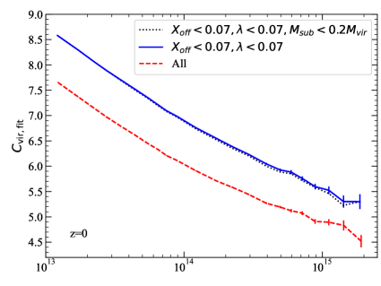
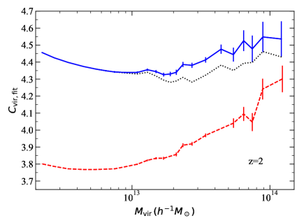
Figure 14: Comparison of concentrations of massive relaxed and all halos at $z=0$ (top panel) and $z=2$ (bottom panel). Here we use virial masses and concentrations. The full curves show concentrations of halos restricted by the offset parameter $X_{\rm off}<0.07$ and spin parameter $\lambda<0.07$. The dotted curves are for halos with an extra condition: we remove halos with the most massive subhalo exceeding 20 per cent of the mass of the central halo. The error bars show the statistical uncertainties of the average values of the concentrations. Note the dramatic difference between $z=0$ and $z=2$ concentrations: no upturn at $z=0$ and a prominent upturn at $z=2$. The upturn is weaker but still present for relaxed halos regardless of which of the two sets of conditions are used. For all redshifts and halo masses, halo concentration is larger for relaxed halos compared with the full population.

One of the contentious issues in this field is the existence and nature of an upturn in the halo concentration–halo mass relation at the massive end. It was first discovered by Klypin et al. (2011) and later confirmed by Prada et al. (2012); Dutton & Macciò (2014); Diemer & Kravtsov (2015); Klypin et al. (2016); Diemer & Joyce (2019). There is a general consensus that the phenomenon is real as far as the population of all halos is concerned. However, there are widely different opinions regarding its nature.

Analytical models for the evolution of halo concentrations so far do not help us understand the nature of the upturn. Those used by Prada et al. (2012) and Diemer & Kravtsov (2015); Diemer & Joyce (2019) assume the upturn, so it is not an argument in favor of it. Models that relate the evolution of the halo concentration with the mass accretion history (Bullock et al., 2001; Zhao et al., 2009; Correa et al., 2015) assume that the concentration increases as the halo accretes mass after an episode of major merger. Again, these models do not predict the upturn. The problem is that mass accretion history is not the only factor that defines halo concentration. Simulations of Klypin et al. (2016) clearly show that halos at the upturn have much more radial orbits when compared with halos at the declining branch of the concentration-mass relation (see, for example, Figure 14 in Klypin et al. (2016)). In turn, large radial velocities of dark matter particles result in more mass reaching small radii, which is the reason for increased concentration. We find the same effect in the Uchuu simulation.

Finding the upturn in cosmological simulations is a difficult numerical problem because it requires relatively high mass resolution and a very large simulation box to have enough statistics of massive halos. For example, Correa et al. (2015) did not find the upturn in either the total population or in relaxed halos. However, their largest computational box was only 400$\,h^{-1}\rm Mpc$. The only chance for them to see the upturn was at $z=2$: at lower redshifts the upturn is weaker and at higher redshifts their computational box and mass resolution are too small to resolve the required population. The largest halos at $z=2$ in Correa et al. (2015) had mass $\sim 10^{13}$$\,h^{-1}\rm M_{\odot}$, and statistical uncertainties for the concentration of these halos was $\sim 10$ percent. They did not see the upturn because it starts at masses larger than $M=10^{13}$$\,h^{-1}\rm M_{\odot}$ (see Figures 9 and 14).

A similar situation happens for simulations of Dutton & Macciò (2014) who had larger box of 1$\,h^{-1}\rm Gpc$ (with thus improved statistics), but a mass resolution of $4\times 10^{11}$$\,h^{-1}\rm M_{\odot}$. Thus, again we do not expect them to see the upturn because their largest halo of $M=2\times 10^{13}$$\,h^{-1}\rm M_{\odot}$ had only 50 particles – not enough to estimate the concentration. Other boxes with better mass resolution were too small to definitively find the upturn.

Our results for relaxed halos contradict those of Ludlow et al. (2012) who argue that once unrelaxed halos are removed, the concentration of the remaining massive halos declines, resulting in the disappearance of the upturn (see their Figure 1). When we remove unrelaxed halos in Uchuu simulation, the concentration increases for all halos including those in the upturn. It is interesting to explore why we have such disagreements. Ludlow et al. (2012) used three conditions to select "relaxed halos": $2K/|W|<1.3$, $X_{\rm off}<0.07$ and the fraction of mass in subhalos $f_{\rm sub}<0.1$. At first sight, these conditions are similar to what we use in Figure 14. As discussed above, as a test we also implemented the condition $f_{\rm sub}<0.1$, but it did not make much of a difference. In spite of the seemingly similar conditions the overall disagreement with Ludlow et al. (2012) is quite dramatic. This can be illustrated by comparing the fractions of relaxed halos at $z=2-3$. In Uchuu simulation, this fraction is about 30 per cent once we add a constraint on the mass of subhalos. In the case of Ludlow et al. (2012), their fraction of relaxed halos was significantly smaller: 2 per cent at $z=3$ and 11 percent at $z=1$. The reason for the small fraction of relaxed halos is due to smaller cutoff of the virial parameter used by Ludlow et al. (2012). As discussed in Sec. 3.5, without a correction for the surface pressure the virial parameter provides very biased results, giving the impression that most of the high-redshift massive halos are out of virial equilibrium, while in reality they are not. Figures 5 and 6 in Klypin et al. (2016) show the effect of this surface pressure correction, which has a strong dependence on redshift. At $z=3$, the vast majority of halos would violate the condition $2K/|W|<1.3$ used by Ludlow et al. (2012), and thus are considered unrelaxed. After the correction, most of them pass this condition and become "relaxed enough" again. Thus we can conclude that the disagreement with Ludlow et al. (2012) is due to an unrealistic constraint on the virial parameter used in their analysis.

We can also now settle another issue: is there an upturn at $z=0$? The argument for the presence of late-redshift upturn was always statistically questionable. With the large volume of the Uchuu simulation we can clearly state that there is no $z=0$ upturn.

4 Summary and Future Prospects

Ongoing and upcoming wide and deep surveys will provide vast amounts of data on galaxies and AGN over Gpc scales. To get as much information as possible from such surveys, precise mock galaxy and AGN catalogues are needed. For this purpose, we conducted a suite of ultra-large cosmological N-body simulations, the Uchuu simulation suite, and constructed halo/subhalo merger trees for them. The largest simulation in the suite, Uchuu, consists of $12800^{3}$ dark matter particles in a box of 2.0$\,h^{-1}\rm Gpc$, with particle mass $3.27\times 10^{8}$$\,h^{-1}\rm M_{\odot}$. The highest resolution simulation in the suite, Shin-Uchuu, consists of $6400^{3}$ particles in a 140$\,h^{-1}\rm Mpc$ box, with particle mass $8.97\times 10^{5}$$\,h^{-1}\rm M_{\odot}$. By combining these simulations, we can follow the evolution of dark matter halos (and subhalos) spanning the mass range from dwarf galaxies to massive galaxy clusters. Thanks to its large volume and high mass resolution, our simulation suite provides one of the the most accurate theoretical templates to date to construct galaxy and AGN catalogues.

In this paper, we have presented the basic properties of the Uchuu suite, which includes halo demographics, the matter power spectra, and halo and subhalo mass functions. These demonstrate the very large dynamic range and superb statistics of the Uchuu simulations. Then we provided an accurate model of halo concentrations that describes our simulations. The results are summarized as follows.

1. From the analysis of the evolution of power spectra, we have demonstrated that our simulations are accurate for use across a wide dynamic range, from the Baryon Acoustic Oscillation scale down to very small structures.

2. We have shown the halo mass function with a mass range spanning approximately eight orders of magnitude, reflecting the power of our very large simulation set. The convergence between simulations is remarkably good – within a few per cent – ensuring the accuracy of our results.

3. The subhalo mass function, with $M_{\rm acc}/M_{\rm vir}$ ranging about six orders of magnitude, is in good agreement with previous simulation work and various model predictions. Yet, our superb statistics reveal a clear difference at the high-mass exponential tail, with a shallow decline towards higher $M_{\rm acc}/M_{\rm vir}$ values.

4. Using the Uchuu suite, we have calibrated the parameters of the halo concentration evolution model presented in Diemer & Joyce (2019). Our fitting errors are within 5 per cent for halos with masses spanning nearly eight orders of magnitude and covering the redshift range $0\leq z\leq 14$.

5. We confirm that there is an upturn in the mass-concentration relation for the population of all halos and of relaxed halos at redshifts $z\gtrsim 0.5$. There is no upturn at lower redshifts.

The data products used in this paper form part of the Uchuu public data release 1, and can be found at http://skiesanduniverses.org/. This includes subsets of simulation particles, matter power spectra, halo/subhalo catalogues, and their merger trees. The latter will be described in an upcoming publication, and are produced by postprocessing the data with the well established tools rockstar (Behroozi et al., 2013a) and consistent trees (Behroozi et al., 2013b). Particle data is provided in the gadget-ii format (Springel, 2005); selected other products use the hdf5 format to help reduce reading and analysis times. This public data release increases the accessibility and portability of our data provides new opportunities for scientific exploitation.

The superb numerical resolution achieved by the Uchuu simulations over an extremely wide halo mass range makes them uniquely powerful to characterize the subhalo population in great detail as well. Indeed, in a forthcoming publication (Moliné et al. in preparation) the full set of Uchuu simulations in Table 1, together with the Phi-4096 high-resolution simulation described in Table 1, will be used to study subhalo concentrations, abundances and distributions. Potential dependencies of subhalo properties with, e.g., host halo mass or distance to host halo centre will also be explored. All together, we anticipate that Uchuu and Phi-4096 will allow us to test, under the same consistent framework, subhalo maximum circular velocities as low as $\rm\sim 1~{}km/s$ and as high as $\rm\sim 1800~{}km/s$ or, equivalently, subhalo masses between $\sim 10^{5}-10^{15}$ $h^{-1}M_{\odot}$, with unprecedented statistics. This impressive subhalo mass range will thus enable the study of halo hierarchy over several orders of magnitude, indeed reaching subhalos as light as $10^{-7}$ the mass of their hosts for some halos. In addition to its inherent cosmological value, this upcoming work on Uchuu halo substructure will be of particular interest to a large variety of topics currently under debate and scrutiny in adjacent fields. For instance, it may serve to elucidate the precise role of subhalos for dark matter searches, e.g., Ackermann et al. (2012); Sánchez-Conde & Prada (2014); Moliné et al. (2017); Coronado-Blázquez et al. (2019); Ishiyama & Ando (2020); or to shed further light on the actual survival of subhalos within their hosts (van den Bosch et al., 2018; van den Bosch & Ogiya, 2018; Meneghetti et al., 2020).

The Uchuu suite of simulations will be used to produce a number of gravitational lensing studies and publicly available products. Light cones of three different sizes (640, 340 and 123 deg²) and depths have been constructed from the simulation snapshots and projected onto a series of shells. Ray-tracing through these cones using a modified version of the glamer (Metcalf & Petkova, 2014; Petkova et al., 2014) code has been done to produce maps of shear, convergence and deflection for a range of source redshifts from 0 to 7 with one arcsecond resolution. For DR1, these maps are being made public along with accurate shear power spectra, correlation functions and the halo-shear correlations. In addition, source catalogs with random positions and known redshift distributions will be provided so that users can sample from them for Monte Carlo calculations. In further data releases, with semi-analytic and Halo Occupation Distribution (HOD) models for the galaxies and inter-cluster baryons, we will produce galaxy-shear lensing predictions and strong lensing statistics for surveys such as Euclid. These results will be presented in a series of companion papers.

Mock catalogs constructed using three semi-analytic models, $\nu^{2}$GC (Makiya et al., 2016; Shirakata et al., 2019), SAG (Cora et al., 2018), and SAGE (Croton et al., 2016) will be released as DR2 in the near future. All data will be made publicly available on http://skiesanduniverses.org/.

Data Availability

As data release 1, we release various $N$-body products for the Uchuu suite on http://skiesanduniverses.org/, such as subsets of simulation particles, matter power spectra, halo/subhalo catalogues, and their merger trees. Non-public data are available upon request. Under the UchuuProject on Github , we provide a collection of general tools for the community, codes / scripts / tutorials and Jupyter notebooks for the analysis of the Uchuu data.

Appendix A How accurate are estimates of halo concentration?

Here we investigate the accuracy of our methods to estimate halo concentration. We start with random realizations of dark matter halos having either NFW or Einasto density profiles. We then proceed by measuring concentrations using averaged halo profiles from the Uchuu simulation at $z=0$ and $z=1.4$. These results are compared between the Uchuu, Shin-Uchuu, and Phi-4096 simulations, each having significantly different mass resolution.

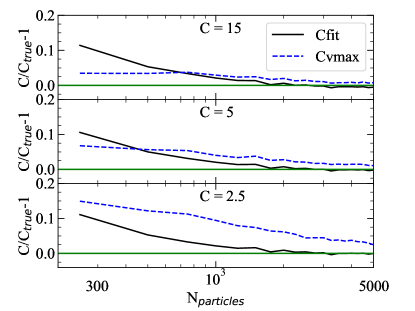
Figure 15: Accuracy of recovering the concentration for halos with random realizations of the NFW density profile. The difference between the measured and true concentration is dependent on the number of halo particles $N_{\rm particles}$, the input concentration $C_{\rm true}$, and the measurement method. For very small number of particles ($N_{\rm particles}\mbox{${\,\hbox{\hbox{$<$}\kern-8.00003pt\lower 4.30554pt\hbox{$\sim$}}\,}$}500$), the $V_{\rm max}$ method provides more accurate results. For a large number of particles ($N_{\rm particles}\mbox{${\,\hbox{\hbox{$>$}\kern-8.00003pt\lower 4.30554pt\hbox{$\sim$}}\,}$}3000$), fitting the density profile gives better results. Overall the differences are small for concentration $C\mbox{${\,\hbox{\hbox{$>$}\kern-8.00003pt\lower 4.30554pt\hbox{$\sim$}}\,}$}3$, and less than $\sim 2$ per cent for $C_{\rm true}>5$ and $N_{\rm particles}>3000$.

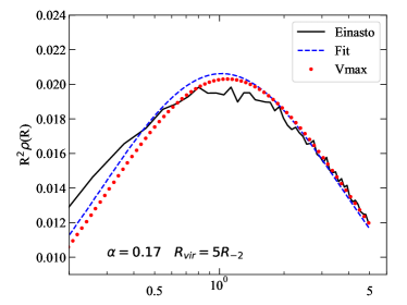
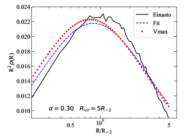
Figure 16: Two examples of fitting Einasto profiles with the NFW profile and using two methods to measure the concentration. Parameters of the Einasto profile are indicated in the panels. For both cases a halo single realization with 300,000 particles was used. The profile in the top panel has a shape parameter $\alpha=0.17$ that can be reasonably well approximated by the NFW profile for radii $R\mbox{${\,\hbox{\hbox{$>$}\kern-8.00003pt\lower 4.30554pt\hbox{$\sim$}}\,}$}0.1R_{\rm vir}$. Indeed, the error in density at those distances are less than $\sim 5$ per cent. Both methods provide similar quality fits. The bottom panel shows the case of large shape parameter, $\alpha=0.3$, which is typical for very massive halos that form in high $\nu=\delta_{\rm c}/\sigma(M)\approx 4$ density peaks. The $V_{\rm max}$ method provides a better approximation for the outer region $R>0.1R_{\rm vir}$, while the direct fitting method is slightly better in the center. In both cases, the error on the density is $\sim 10$ per cent for $R>0.1R_{\rm vir}$. Density is shown in arbitrary units.

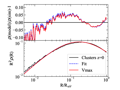
Figure 17: Fitting the halo density profile of $M_{\rm vir}=1.5\times 10^{15}$$\,h^{-1}\rm M_{\odot}$ halos at $z=0$ with the NFW profile. The true halo profile was obtained by averaging the profiles of 100 halos of this mass in the Uchuu simulation. Both halo concentration measurement methods provide nearly identical fits, with a $\sim 5$ per cent accuracy for $R=(0.01-1)R_{\rm vir}$. The lower panel shows $R^{2}\rho(R)$ in arbitrary units.

A.1 Random realizations of NFW halos

This is a simple test: make a random realization of a NFW halo with a given concentration and some number of particles. Because, by design, the concentration $C_{\rm true}$ is known, ideally the algorithm should find it. However, there is always noise in any such measurement due to the finite number of particles, and the algorithm may produce biased estimates.

We approximately follow the procedure used by the rockstar halo finder (Behroozi et al., 2013a). All particles are sorted by distance. Binning is done by constant mass so that each interval has the same number of particles (S/N). The total number of bins is 50. However the first bin is special: it always has 15 particles. We then measure the density and circular velocity for each bin. A density profile is then fitted using the NFW profile, providing a concentration value $C_{\rm fit}$. Similarly, a circular velocity curve is used to find $V_{\rm max}$, leading to an estimate of a concentration value $C_{\rm vmax}$. Many realizations (typically 300) are performed to find the average and rms measurement of each true concentration.

Figure 15 present $C/C_{\rm true}$ as a function of particle number for each method. The three panels show three selected values for the true concentration: $C_{\rm true}=15$ for high concentration halos like our Milky Way, $C_{\rm true}=5$ for intermediate halos, and $C_{\rm true}=2.5$ for very low concentrations, close to the minimum concentration of the simulations at high redshifts. The deviation from the true value is found to depend on the number of particles $N_{\rm particles}$, the input concentration $C_{\rm true}$, and the method used. For very small particle number ($N_{\rm particles}\mbox{${\,\hbox{\hbox{$<$}\kern-8.00003pt\lower 4.30554pt\hbox{$\sim$}}\,}$}500$) the $V_{\rm max}$ method provides more accurate results. For large particle number ($N_{\rm particles}\mbox{${\,\hbox{\hbox{$>$}\kern-8.00003pt\lower 4.30554pt\hbox{$\sim$}}\,}$}3000$) fitting the density profile gives better results. However the differences are small for concentrations $C\mbox{${\,\hbox{\hbox{$>$}\kern-8.00003pt\lower 4.30554pt\hbox{$\sim$}}\,}$}3$, and less than $\sim 2$ per cent for $C_{\rm true}>5$ and $N_{\rm particles}>3000$. The only substantial errors happen at very low concentration where $C_{\rm max}$ can be systematically above the true values by 10-15 per cent. The main reason for this is related to the fact that the radius corresponding to $V_{\rm max}$ is very close to the radius of the halo, and fluctuations are amplified producing an upward biased estimate.

The main take away of this test is that both methods produce nearly the same estimates of the true concentration if the density profile is NFW and the number of particles are more than 3000.

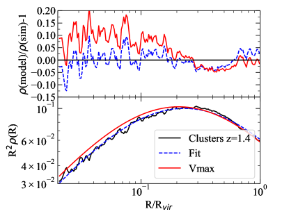
Figure 18: Fitting the halo profile of $M_{\rm vir}=1.5\times 10^{14}$$\,h^{-1}\rm M_{\odot}$ halos at $z=1.4$ with the NFW profile. The true halo profile was obtained by averaging the profiles of 100 halos of this mass in the Uchuu simulation. Both halo concentration measurement methods provide nearly identical fits in the outer halo region $R=(0.2-1)R_{\rm vir}$, accurate to $\sim 5$ per cent, while the fitting procedure does better in the center. The lower panel shows $R^{2}\rho(R)$ in arbitrary units.

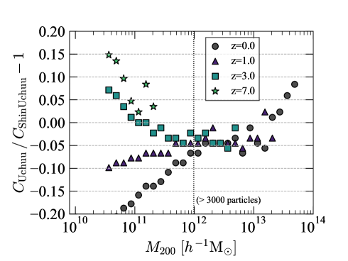
Figure 19: Relative residuals of the median values of halo concentration $c_{200}$, comparing the Shin-Uchuu (higher resolution) and Uchuu (lower resolution) simulations, at $z=0.0,1.0,3.0$, and $7.0$. Concentrations are measured using the $V_{\rm max}$ method. The vertical dotted line corresponds to a halo mass with 3,000 particles in the Uchuu simulation. At this point, residuals become larger with decreasing halo mass.

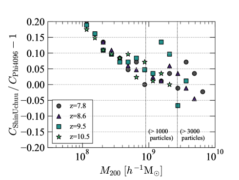
Figure 20: Relative residuals of the median values halo concentrations $c_{200}$, comparing the Phi-4096 (higher resolution) and Shin-Uchuu (lower resolution) simulations, at $z=7.8,8.6,9.5$, and $10.5$. Concentrations are measured using the $V_{\rm max}$ method. The vertical dotted lines corresponds to a halo mass with 1,000 and 3,000 particles in the Shin-Uchuu simulation.

A.2 Random realizations of Einasto halos

Halos typically have profiles that are better approximated by the more general Einasto profile. The Einasto profile has three parameters, controlling the mass via $\rho_{0}$, the radius $R_{-2}$ where the log-log density slope is -2, and the shape parameter $\alpha$, which roughly describes the width of the profile. It has the functional form

$$\rho(R)=\rho_{0}\exp\left[-\frac{2}{\alpha}\left(x^{\alpha}-1\right)\right],\quad x\equiv R/R_{-2}.$$ (4)

Figure 16 gives the example of two Einasto profiles with different shape parameters. In the top panel we show $\alpha=0.17$, which is typical for galaxy-size halos. Such halos have a relatively broad profile and are reasonably accurately fitted by the NFW profile. In the bottom panel we show $\alpha=0.30$, which is more characteristic of massive clusters or, in general, for high peaks in the initial density field. Because the shape of such halos are not NFW, there is no true concentration using the formal definitions. However, we can still apply our methods and see how accurately the density profile is described.

Not surprisingly, fits for $\alpha=0.17$, while not perfect, are relatively good. The errors where the density profile peaks (at 1/5 the halo radius) are approximately 5 per cent and increase towards very small radii. The two methods of measuring concentration produce different estimates at the 20 per cent level. However, it is not clear which one is better overall. We find the $V_{\rm max}$ method provides a slightly improved fit in the outer regions of the halo, while the fitting method is better towards the halo center.

The $\alpha=0.30$ halo is much more difficult to compare because the halo profile is far from NFW. The methods produce different concentrations, with $V_{\rm max}$ predicting higher concentration and smaller errors in the outer regions.

A.3 Average profiles of massive halos in the Uchuu simulation

Here we extend the above analysis to real halos, and measure concentrations using the averaged profiles of massive relaxed halos selected from a narrow mass interval. We define a halo to be relaxed if its offset parameter (the distance between the halo center and halo center of mass, measured in units of the virial radius) is less than 0.05, and its spin parameter less than 0.03. This is done to remove halos that experience significant non-equilibrium events. Averaging over many halos of the same mass serves the same purpose as smoothing substructures. Results are presented in Figures 17 and 18 for $100$ clusters at $z=0$ and $z=1.4$.

At $z=0$ both methods of measuring concentration produced very close estimates. Note that the halo profile we find itself is not a NFW; there are $\sim 5$ per cent systematic deviations. The errors and the shape of the average halo profile is different at $z=1.4$ compared with $z=0$. Here, the fitting method works better except at the very outer 20 per cent region near the virial radius. The difference in concentration produced by the two methods is about 10 per cent, with the $V_{\rm max}$ method predicting higher concentration.

A.4 The convergence of halo concentrations

Because we have three simulations with vastly different force and mass resolutions, we can compare estimates of halos concentration for halos of the same mass found in different simulations. We can also investigate the minimum number of particles per halo that is required to determine the halo concentration robustly.

Figure 19 shows the relative residuals of median concentration between the Uchuu and the Shin-Uchuu simulations as a function of halo mass. The difference is less than around 5 per cent for halos more massive than $\sim 10^{12}$$\,h^{-1}\rm M_{\odot}$, corresponding to 3,000 particles in the Uchuu simulation. For less massive halos, the difference increases regardless of the halo mass. Therefore, we conclude that 3,000 particles per halo is the minimum threshold for the Uchuu simulation to robustly measure concentration.

Figure 20 shows the relative residuals of median concentration between the Shin-Uchuu and the Phi-4096 simulations as the function of halo mass. Differences can be seen to increase systematically below $\sim 9.0\times 10^{8}$$\,h^{-1}\rm M_{\odot}$, corresponding to 1,000 particles in the Shin-Uchuu simulation. For more massive halos the difference is less than 5 per cent, except at $z=9.5$ where the scatter is large due to poor statistics in the Phi-4096 simulation. However, we observe no systematic trend. Therefore, we consider 1,000 particles per halo is the minimum threshold for the Shin-Uchuu simulation to robustly measure concentration. This value is smaller than that for the Uchuu simulation, reflecting that the softening length of Shin-Uchuu is much smaller. We also use this threshold for the Phi-4096 simulation because the ratio of mean particle separation to softening length is close to that of the Shin-Uchuu simulation.

Appendix B Analytical model of mass-concentration relation

Following Diemer & Joyce (2019), we model halo concentration using the analytical approximation

$$c(\nu,n_{\rm eff},\alpha_{\rm eff})=C\left(\alpha_{\mathrm{eff}}\right)\times\tilde{G}\left(\frac{A\left(n_{\mathrm{eff}}\right)}{\nu}\left[1+\frac{\nu^{2}}{B\left(n_{\mathrm{eff}}\right)}\right]\right),$$ (5)

where $\tilde{G}(x)$ is the inverse function of

$$G(x)=\frac{x}{[f(x)]^{\left(5+n_{\mathrm{eff}}\right)/6}}.$$ (6)

Here, $f(x)=\ln(1+x)-x/(1+x)$ is the mass function of the NFW profile, $\nu=\delta_{\rm c}/\sigma(M)$ is the height of the density peak, $\delta_{\rm c}=1.686$ is the critical over-density for spherical collapse, and $\sigma(M)$ is the rms density fluctuation. Variables $n_{\rm eff}$ and $\alpha_{\rm eff}$ are defined as

$$n_{\mathrm{eff}}(M)=-\left.2\frac{d\ln\sigma(R)}{d\ln R}\right|_{R=\kappa R_{\mathrm{L}}}-3,$$ (7)

and

$$\alpha_{\mathrm{eff}}(z)=-\frac{d\ln D(z)}{d\ln(1+z)}.$$ (8)

The latter is the effective exponent of linear growth $D(z)$. The former reflects the effective slope of the power spectrum, $\sigma(R)$ is the rms density fluctuation in spheres with Lagrangian radius $R_{\rm L}$ multiplied by a free parameter $\kappa$. Halo mass $M$ is directly related to $R_{\rm L}$ through

$$M=\frac{4\pi}{3}\rho_{m}R_{\rm L}^{3},$$ (9)

where $\rho_{m}(z=0)$ is the mean density at $z=0$. Terms $A(n_{\rm eff})$, $B(n_{\rm eff})$, and $C(\alpha_{\rm eff})$ in Equation 5 have the following form:

$$\begin{array}[]{l}A\left(n_{\mathrm{eff}}\right)=a_{0}\left(1+a_{1}\left(n_{\mathrm{eff}}+3\right)\right),\\ B\left(n_{\mathrm{eff}}\right)=b_{0}\left(1+b_{1}\left(n_{\mathrm{eff}}+3\right)\right),\\ C\left(\alpha_{\mathrm{eff}}\right)=1-c_{\alpha}\left(1-\alpha_{\mathrm{eff}}\right),\end{array}$$ (10)

with free parameters $a_{0},a_{1},b_{0},b_{1}$, and $c_{\alpha}$.

Appendix C Mass-concentration relation for relaxed halos and for overdensity 500 halo definition

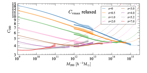
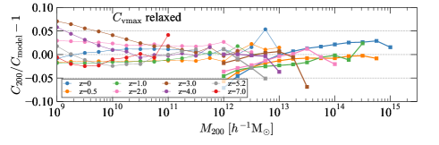
Figure 21: Concentrations for relaxed halos using $V_{\rm max}$ method. (eq.(1)) Top panel: Mass-concentration relation of relaxed halos for the Uchuu (thick curves) and the Shin-Uchuu (thin curves) simulations. The dashed curves are predictions of the analytical model described by eq. (2). Bottom panel: The fractional difference between the halo concentrations of the Uchuu (squares) and the Shin-Uchuu (circles) simulations and the model predictions.

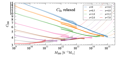
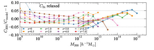
Figure 22: The same as in Figure 21 but for concentrations estimated by profile fitting.

Figure 21 shows the mass-concentration relation of the Uchuu and Shin-Uchuu simulations and their redshift evolution for only relaxed halos. The concentrations are estimated using the $V_{\rm max}$ method (eq.(1)). Overall trend is the same as the relation for all halos (Figure 9). The concentration for relaxed halos shows a well-known behaviour that relaxed halos have larger concentrations. Even for relaxed halos, we observe a flattening and an upturn with increasing mass, consistent with Klypin et al. (2016). Figure 22 also shows the mass-concentration relation, where concentrations are estimated by the profile fitting. The plot shows that the main tendencies of the concentration-mass relations do not depend on the method to find concentration. This includes the upturn in the concentration at large masses.

Bottom panels of Figure 21 and 22 show residuals of concentrations from the model. The accuracy level is similar to those for all halos (Figure 9 and 10). We also confirm that the accuracy level is also comparable at mass $M_{200}<10^{11}$$\,h^{-1}\rm M_{\odot}$ and redshift $z>7$. We also provide best fitting parameters of the mass-concentration relation with $c_{500}$ estimated by profile fitting in Table 2 and show the result in Figure 23.

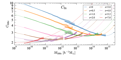
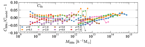
Figure 23: Evolution of concentration-mass relation for all halos. Concentrations are estimated by profile fitting and for the halo mass and concentration defined using $r_{500}$, in which the average spherical overdensity is 500 times the critical density. Labeling of curves is the same as in Figure 21.

Appendix D Validation of merger trees

Our use of consistent trees needed to be modified to make merger tree construction possible on simulations of the size of those in the Uchuu suite. As explained in §2, to overcome this hurdle, we split the full box of each simulation into smaller regularly spaced sub-volumes, and ran consistent trees for each sub-volume separately. In this Section, we compare merger trees of the mini-Uchuu simulation constructed by this method and the original consistent trees code in order to show the robustness of this method.

A number of metrics have been used to evaluate merger trees such as length of tree and mass growth history of halos (e.g., Srisawat et al., 2013), and merger rate. Visualization tools have also been provided (e.g., Smith & Lang, 2019; Poulton et al., 2018). Here, we use mean merger rate because mergers trigger a number of events in semi-analytic galaxy models. Given a halo with mass $M_{i}$ at redshift $z_{i}$, we define the merger mass ratio $\xi=M_{i-1,j}/M_{i-1,0}$, where $i$ and $j$ denote the snapshot id and progenitors of the halo, respectively. We set the progenitor with $j=0$ to be the most massive progenitor and compute the number of mergers per halo as a function of $z_{i}$, $\xi$ and the descendant halo mass $M_{i}$.

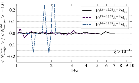
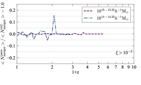
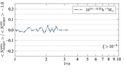
Figure 24: Comparison of mean merger rate of trees of the mini-Uchuu simulation constructed by our method ($\langle N^{\rm para}_{\rm merger}\rangle$) described in § 2 and the original consistent trees code ($\langle N^{\rm std}_{\rm merger}\rangle$) as a function of redshift for three halo mass ranges, and three merger mass ratios $\xi$.

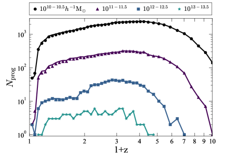
Figure 25: Total number of progenitor halos and subhalos $N_{\rm prog}$ of the tree of the largest halo at $z=0$ in the mini-Uchuu simulation as a function of redshift for four progenitor mass ranges. Symbols denote results of our method, and solid curves denote those of the original consistent trees code.

Figure 24 shows the comparison of mean merger rate of trees of the mini-Uchuu simulation constructed by our method ($\langle N^{\rm para}_{\rm merger}\rangle$) and the original consistent trees code ($\langle N^{\rm std}_{\rm merger}\rangle$) as a function of redshift for three halo mass bin and three merger mass ratio. Except for the most massive halo mass ($10^{14-14.25}$$\,h^{-1}\rm M_{\odot}$), the difference of both methods is always within five per cent, ensuring the accuracy of our method. For halos with $10^{14-14.25}$$\,h^{-1}\rm M_{\odot}$, both merger rates converge well within five per cent level with little exceptions. There are four spots for $\xi>10^{-1}$ and one spot for $\xi>10^{-2}$, where the difference exceeds ten per cent. This is because such mergers with massive halos are rare and the number difference at each redshift is only one. Thus, this large difference in ratio is not significant.

We also perform a stricter test. Figure 25 shows the comparison of the total number of progenitor halos and subhalos of the tree of the largest halo ($\sim 2.0\times 10^{15}$$\,h^{-1}\rm M_{\odot}$) at $z=0$ in the mini-Uchuu simulation as a function of redshift for four progenitor mass ranges. The number of progenitors agrees well with each other for progenitor mass more massive than $10^{12}$$\,h^{-1}\rm M_{\odot}$. For less massive progenitors there are small deviations, but which are typically only less than five percent level. We conclude that merger trees constructed by our method are equivalent to those obtained from the original consistent trees code.

References

- Ackermann et al. (2012) Ackermann M., et al., 2012, ApJ, 747, 121
- Behroozi et al. (2010) Behroozi P. S., Conroy C., Wechsler R. H., 2010, ApJ, 717, 379
- Behroozi et al. (2013a) Behroozi P. S., Wechsler R. H., Wu H.-Y., 2013a, ApJ, 762, 109
- Behroozi et al. (2013b) Behroozi P. S., Wechsler R. H., Wu H.-Y., Busha M. T., Klypin A. A., Primack J. R., 2013b, ApJ, 763, 18
- Benson (2012) Benson A. J., 2012, New Astron., 17, 175
- Berlind & Weinberg (2002) Berlind A. A., Weinberg D. H., 2002, ApJ, 575, 587
- Bullock et al. (2001) Bullock J. S., Kolatt T. S., Sigad Y., Somerville R. S., Kravtsov A. V., Klypin A. A., Primack J. R., Dekel A., 2001, MNRAS, 321, 559
- Cheng et al. (2020) Cheng S., Yu H.-R., Inman D., Liao Q., Wu Q., Lin J., 2020, arXiv e-prints, p. arXiv:2003.03931
- Child et al. (2018) Child H. L., Habib S., Heitmann K., Frontiere N., Finkel H., Pope A., Morozov V., 2018, ApJ, 859, 55
- Collette (2013) Collette A., 2013, Python and HDF5. O’Reilly
- Conroy et al. (2006) Conroy C., Wechsler R. H., Kravtsov A. V., 2006, ApJ, 647, 201
- Cooray & Sheth (2002) Cooray A., Sheth R., 2002, Phys. Rep., 372, 1
- Cora et al. (2018) Cora S. A., et al., 2018, MNRAS, 479, 2
- Coronado-Blázquez et al. (2019) Coronado-Blázquez J., Sánchez-Conde M. A., Domínguez A., Aguirre-Santaella A., Mauro M. D., Mirabal N., Nieto D., Charles E., 2019, Journal of Cosmology and Astroparticle Physics, 2019, 020
- Correa et al. (2015) Correa C. A., Wyithe J. S. B., Schaye J., Duffy A. R., 2015, MNRAS, 452, 1217
- Crocce et al. (2006) Crocce M., Pueblas S., Scoccimarro R., 2006, MNRAS, 373, 369
- Croton et al. (2006) Croton D. J., et al., 2006, MNRAS, 365, 11
- Croton et al. (2016) Croton D. J., et al., 2016, ApJS, 222, 22
- Davis et al. (2011) Davis A. J., D’Aloisio A., Natarajan P., 2011, MNRAS, 416, 242
- Despali et al. (2016) Despali G., Giocoli C., Angulo R. E., Tormen G., Sheth R. K., Baso G., Moscardini L., 2016, MNRAS, 456, 2486
- Diemer (2018) Diemer B., 2018, ApJS, 239, 35
- Diemer & Joyce (2019) Diemer B., Joyce M., 2019, ApJ, 871, 168
- Diemer & Kravtsov (2015) Diemer B., Kravtsov A. V., 2015, ApJ, 799, 108
- Dolag et al. (2015) Dolag K., Gaensler B. M., Beck A. M., Beck M. C., 2015, MNRAS, 451, 4277
- Dubois et al. (2014) Dubois Y., et al., 2014, MNRAS, 444, 1453
- Dutton & Macciò (2014) Dutton A. A., Macciò A. V., 2014, MNRAS, 441, 3359
- Hahn & Abel (2011) Hahn O., Abel T., 2011, MNRAS, 415, 2101
- Hahn et al. (2013) Hahn O., Abel T., Kaehler R., 2013, MNRAS, 434, 1171
- Hiroshima et al. (2018) Hiroshima N., Ando S., Ishiyama T., 2018, Phys. Rev. D, 97, 123002
- Hunter (2007) Hunter J. D., 2007, Computing in Science Engineering, 9, 90
- Ishiyama & Ando (2020) Ishiyama T., Ando S., 2020, MNRAS, 492, 3662
- Ishiyama et al. (2009) Ishiyama T., Fukushige T., Makino J., 2009, PASJ, 61, 1319
- Ishiyama et al. (2012) Ishiyama T., Nitadori K., Makino J., 2012, in Proc. Int. Conf. High Performance Computing, Networking, Storage and Analysis, SC’12 (Los Alamitos, CA: IEEE Computer Society Press), 5:, (arXiv:1211.4406). http://dl.acm.org/citation.cfm?id=2388996.2389003
- Ishiyama et al. (2015) Ishiyama T., Enoki M., Kobayashi M. A. R., Makiya R., Nagashima M., Oogi T., 2015, PASJ, 67, 61
- Klypin & Prada (2018) Klypin A., Prada F., 2018, MNRAS, 478, 4602
- Klypin et al. (2011) Klypin A. A., Trujillo-Gomez S., Primack J., 2011, ApJ, 740, 102
- Klypin et al. (2016) Klypin A., Yepes G., Gottlöber S., Prada F., Heß S., 2016, MNRAS, 457, 4340
- Knebe et al. (2013) Knebe A., et al., 2013, MNRAS, 435, 1618
- Knebe et al. (2018) Knebe A., et al., 2018, MNRAS, 474, 5206
- Kravtsov et al. (2004) Kravtsov A. V., Berlind A. A., Wechsler R. H., Klypin A. A., Gottlöber S., Allgood B. o., Primack J. R., 2004, ApJ, 609, 35
- Laureijs et al. (2011) Laureijs et al. R., 2011, arXiv e-prints, p. arXiv:1110.3193
- Leauthaud et al. (2012) Leauthaud A., et al., 2012, ApJ, 744, 159
- Lewis et al. (2000) Lewis A., Challinor A., Lasenby A., 2000, ApJ, 538, 473
- Ludlow et al. (2012) Ludlow A. D., Navarro J. F., Li M., Angulo R. E., Boylan-Kolchin M., Bett P. E., 2012, MNRAS, 427, 1322
- Makiya et al. (2016) Makiya R., et al., 2016, PASJ, 68, 25
- Mead et al. (2015) Mead A. J., Peacock J. A., Heymans C., Joudaki S., Heavens A. F., 2015, MNRAS, 454, 1958
- Meneghetti et al. (2020) Meneghetti M., et al., 2020, Science, 369, 1347
- Metcalf & Petkova (2014) Metcalf R. B., Petkova M., 2014, MNRAS, 445, 1942
- Miyazaki et al. (2006) Miyazaki S., et al., 2006, in Society of Photo-Optical Instrumentation Engineers (SPIE) Conference Series. , doi:10.1117/12.672739
- Miyazaki et al. (2012) Miyazaki S., et al., 2012, in Society of Photo-Optical Instrumentation Engineers (SPIE) Conference Series. p. 0, doi:10.1117/12.926844
- Moliné et al. (2017) Moliné Á., Sánchez-Conde M. A., Palomares-Ruiz S., Prada F., 2017, MNRAS, 466, 4974
- Moster et al. (2010) Moster B. P., Somerville R. S., Maulbetsch C., van den Bosch F. C., Macciò A. V., Naab T., Oser L., 2010, ApJ, 710, 903
- Navarro et al. (1997) Navarro J. F., Frenk C. S., White S. D. M., 1997, ApJ, 490, 493
- Navarro et al. (2004) Navarro J. F., et al., 2004, MNRAS, 349, 1039
- Neto et al. (2007) Neto A. F., et al., 2007, MNRAS, 381, 1450
- Nitadori et al. (2006) Nitadori K., Makino J., Hut P., 2006, New Astron., 12, 169
- Okoli & Afshordi (2016) Okoli C., Afshordi N., 2016, MNRAS, 456, 3068
- Peacock & Smith (2000) Peacock J. A., Smith R. E., 2000, MNRAS, 318, 1144
- Petkova et al. (2014) Petkova M., Metcalf R. B., Giocoli C., 2014, MNRAS, 445, 1954
- Pilipenko et al. (2017) Pilipenko S. V., Sánchez-Conde M. A., Prada F., Yepes G., 2017, MNRAS, 472, 4918
- Planck Collaboration et al. (2020) Planck Collaboration et al., 2020, A&A, 641, A6
- Potter et al. (2017) Potter D., Stadel J., Teyssier R., 2017, Computational Astrophysics and Cosmology, 4, 2
- Poulton et al. (2018) Poulton R. J. J., Robotham A. S. G., Power C., Elahi P. J., 2018, Publ. Astron. Soc. Australia, 35, 42
- Prada et al. (2012) Prada F., Klypin A. A., Cuesta A. J., Betancort-Rijo J. E., Primack J., 2012, MNRAS, 423, 3018
- Reddick et al. (2013) Reddick R. M., Wechsler R. H., Tinker J. L., Behroozi P. S., 2013, ApJ, 771, 30
- Rodríguez-Puebla et al. (2016) Rodríguez-Puebla A., Behroozi P., Primack J., Klypin A., Lee C., Hellinger D., 2016, MNRAS, 462, 893
- Sánchez-Conde & Prada (2014) Sánchez-Conde M. A., Prada F., 2014, Monthly Notices of the Royal Astronomical Society, 442, 2271
- Schaye et al. (2015) Schaye J., et al., 2015, MNRAS, 446, 521
- Schneider et al. (2016) Schneider A., et al., 2016, J. Cosmology Astropart. Phys., 2016, 047
- Seljak (2000) Seljak U., 2000, MNRAS, 318, 203
- Shankar et al. (2006) Shankar F., Lapi A., Salucci P., De Zotti G., Danese L., 2006, ApJ, 643, 14
- Shaw et al. (2006) Shaw L. D., Weller J., Ostriker J. P., Bode P., 2006, ApJ, 646, 815
- Shirakata et al. (2019) Shirakata H., et al., 2019, MNRAS, 482, 4846
- Skillman et al. (2014) Skillman S. W., Warren M. S., Turk M. J., Wechsler R. H., Holz D. E., Sutter P. M., 2014, arXiv: 1407.2600,
- Smith & Angulo (2019) Smith R. E., Angulo R. E., 2019, MNRAS, 486, 1448
- Smith & Lang (2019) Smith B. D., Lang M., 2019, Journal of Open Source Software, 4, 1881
- Springel (2005) Springel V., 2005, MNRAS, 364, 1105
- Springel et al. (2005) Springel V., et al., 2005, Nature, 435, 629
- Springel et al. (2018) Springel V., et al., 2018, MNRAS, 475, 676
- Srisawat et al. (2013) Srisawat C., et al., 2013, MNRAS, 436, 150
- Takada et al. (2014) Takada et al. M., 2014, PASJ, 66, 1
- Takahashi et al. (2012) Takahashi R., Sato M., Nishimichi T., Taruya A., Oguri M., 2012, ApJ, 761, 152
- Tanikawa et al. (2012) Tanikawa A., Yoshikawa K., Okamoto T., Nitadori K., 2012, New Astron., 17, 82
- Tanikawa et al. (2013) Tanikawa A., Yoshikawa K., Nitadori K., Okamoto T., 2013, New Astron., 19, 74
- Vale & Ostriker (2004) Vale A., Ostriker J. P., 2004, MNRAS, 353, 189
- Virtanen et al. (2020) Virtanen P., et al., 2020, Nature Methods, 17, 261
- Vogelsberger et al. (2014) Vogelsberger M., et al., 2014, MNRAS, 444, 1518
- Vogelsberger et al. (2020) Vogelsberger M., Marinacci F., Torrey P., Puchwein E., 2020, Nature Reviews Physics, 2, 42
- Yoshikawa & Tanikawa (2018) Yoshikawa K., Tanikawa A., 2018, Research Notes of the American Astronomical Society, 2, 231
- Zhao et al. (2009) Zhao D. H., Jing Y. P., Mo H. J., Börner G., 2009, ApJ, 707, 354
- Zheng et al. (2007) Zheng Z., Coil A. L., Zehavi I., 2007, ApJ, 667, 760
- van den Bosch & Ogiya (2018) van den Bosch F. C., Ogiya G., 2018, MNRAS, 475, 4066
- van den Bosch et al. (2018) van den Bosch F. C., Ogiya G., Hahn O., Burkert A., 2018, MNRAS, 474, 3043
- van der Walt et al. (2011) van der Walt S., Colbert S. C., Varoquaux G., 2011, Computing in Science Engineering, 13, 22