Constraints on Primordial Power Spectrum from Galaxy Luminosity Functions

Abstract

We derive constraints on primordial power spectrum, for the first time, from galaxy UV luminosity functions (LFs) at high redshifts. Since the galaxy LFs reflect an underlying halo mass function which depends on primordial fluctuations, one can constrain primordial power spectrum, particularly on small scales. We perform a Markov Chain Monte Carlo analysis by varying parameters for primordial power spectrum as well as those describing astrophysics. We adopt the UV LFs derived from Hubble Frontier Fields data at $z=6-10$, which enable us to probe primordial fluctuations on the scales of $k\sim 10-10^{3}~{}{\rm Mpc}^{-1}$. Our analysis also clarifies how the assumption on cosmology such as primordial power spectrum affects the determination of astrophysical parameters.

I Introduction

Probing primordial power spectrum is of prime importance in understanding the dynamics of the inflationary Universe. While observations of cosmic microwave background (CMB) have measured primordial power spectrum precisely Akrami et al. (2018), only large scales are probed by such observations, which gives us the information on the inflationary dynamics only within some limited period. To elucidate the whole inflationary dynamics, we need to probe primordial fluctuations over a much wider range of scales, which motivates the study to investigate constraints on primordial power spectrum with probes other than CMB, especially on small scales.

When one assumes a standard single-field inflation model, the primordial power spectrum ${\cal P}_{\zeta}(k)$, with $k$ being the wave number for the mode of fluctuations, can be well described by the power-law form as

$${\cal P_{\zeta}}(k)=A_{s}(k_{\ast})\left(\frac{k}{k_{\ast}}\right)^{n_{s}-1},$$ (1)

where $A_{s}(k_{\ast})$ is the amplitude at the reference scale $k_{\ast}$ and $n_{s}$ is the spectral index. However, even for a standard single-field model, $n_{s}$ is not precisely constant, and also in some models, $n_{s}$ is predicted to be scale dependent, which motivates the following description for ${\cal P}_{\zeta}$:

$${\cal P_{\zeta}}(k)=A_{s}(k_{\ast})\left(\frac{k}{k_{\ast}}\right)^{n_{s}-1+\frac{1}{2!}\alpha_{s}\ln\left(\frac{k}{k_{\ast}}\right)+\frac{1}{3!}\beta_{s}\ln\left(\frac{k}{k_{\ast}}\right)^{2}},$$ (2)

where $\alpha_{s}$ and $\beta_{s}$ are the so-called running and the running of the running parameters, respectively. When primordial power spectrum is probed over a wide range of scales, the running parameters can be well constrained due to the lever-arm effect. Furthermore, the primordial power spectrum may not be well described by a simple form such as Eq. (1) or Eq. (2) given that a wide variety of inflationary models have been proposed, some of which do not allow those kind of smooth functional forms to describe ${\cal P}_{\zeta}(k)$. Therefore it would be of great importance to investigate ${\cal P}_{\zeta}(k)$ for a broad range of scales. These considerations motivate us to look into yet other probes of primordial fluctuations, particularly on small scales. Examples of such work include primordial black holes Bugaev and Klimai (2009); Josan et al. (2009); Sato-Polito et al. (2019), ultracompact minihalos Bringmann et al. (2012); Emami and Smoot (2018), neutral hydrogen 21cm fluctuations Kohri et al. (2013); Sekiguchi et al. (2018); Muñoz et al. (2017), 21cm global signal Yoshiura et al. (2018, 2020), CMB spectral distortion Chluba et al. (2012), for which constraints on the small-scale amplitude of primordial power spectrum or the so-called the running and the running of the running parameters are investigated.

In this paper, we derive constraints on primordial power spectrum using galaxy UV luminosity functions (LFs) at high redshifts for the first time. Since the galaxy LF reflects an underlying halo mass function which depends on primordial fluctuations, one can probe primordial power spectrum by using observations of UV LFs. We adopt the LFs at high redshifts of $z=6-10$ determined from Hubble Frontier Fields data Bouwens et al. (2017); Oesch et al. (2018); Ishigaki et al. (2018), which enable us to probe primordial power spectrum on scales much smaller than CMB, around $k\sim 10-10^{3}~{}{\rm Mpc}^{-1}$. With such small scale information, one can directly constrain its amplitude on small scales and also the so-called running and running of the running parameters $\alpha_{s}$ and $\beta_{s}$.

It should be noted that the LF also depends on the assumption for astrophysics such as the fraction of galactic gas converted into stars, star formation rate and so on. To take account of such uncertainties, we perform a Markov Chain Monte Carlo (MCMC) analysis to obtain constraints on primordial power spectrum by varying both the astrophysical parameters and the ones describing primordial power spectrum.

We also emphasize that, although our primary purpose is to derive constraints on primordial power spectrum, our analysis also clarifies to what extent the determination of astrophysical parameters are affected by the assumption on primordial fluctuations. When one tries to investigate astrophysics or constrain astrophysical parameters, the standard $\Lambda$-dominated Cold Dark Matter ($\Lambda$CDM) model with power-law primordial power spectrum is usually assumed. Although almost all cosmological observations are consistent with the standard $\Lambda$CDM model, some deviations from this standard paradigm are still possible, particularly on small scales, since observations such as CMB and galaxy clustering only probe large scales. In the following analysis, we model ${\cal P}_{\zeta}(k)$ to capture its small scale feature keeping large scale power spectrum consistent with current observations including CMB. This modeling enable us to investigate how the assumption on cosmology, especially on small scales, affects the study of astrophysics.

The structure of this paper is as follows. In Section II, we give our formalism to investigate constraints on primordial power spectrum. First we provide how we model primordial power spectrum and what parameters to be constrained. Then we address the formalism to derive constraints on primordial power spectrum using the galaxy luminosity function. In Section III, we show constraints on ${\cal P}_{\zeta}(k)$ for several models from UV LFs at high redshifts. We also discuss how the uncertainties of primordial power spectrum affects the measurements of astrophysical parameters in Section IV. Finally we conclude in Section V.

II Analysis Method

In this section, we summarize the analysis method adopted in this paper. First we present our modeling of primordial power spectrum (PPS) ${\cal P}_{\zeta}$. We then give the formalism to calculate the galaxy UV LFs. The machineries to derive constraints on PPS are also presented, such as the construction of the likelihood function and a Markov Chain Monte Carlo (MCMC) analysis adopted in this paper.

II.1 Modeling of Primordial Power Spectrum

We consider several types of modeling for PPS. The first one is a power-law form which accommodates the scale dependence of the power-law index by using the so-called running parameters:

$${\cal P}_{\zeta}(k)=A_{s}(k_{\ast})\left(\frac{k}{k_{*}}\right)^{n_{s}-1+\frac{1}{2}\alpha_{s}\ln\left(\frac{k}{k_{*}}\right)+\frac{1}{6}\beta_{s}\left(\ln\left(\frac{k}{k_{*}}\right)\right)^{2}},$$

[Parametrization I] (3)

where $n_{s}$ is the spectral index, $\alpha_{s}$ is the running parameter, and $\beta_{s}$ is the running of running parameter. We adopt the reference scale of $k_{*}=0.05\rm Mpc^{-1}$. $A_{s}(k_{\ast})$ is the amplitude at the reference scale $k_{\ast}$. In our analysis, we fix the amplitude at the reference scale as $A_{s}(k_{\ast})=2.105\times 10^{-9}$ so as to be consistent with CMB observations Akrami et al. (2018). We call this modeling as “Parametrization I”.

Other types of modeling are based on the following form:

$${\cal P}_{\zeta}(k) = A_{s}(k_{\ast})\left(\frac{k}{k_{*}}\right)^{n_{s}-1}p(k),$$ (4)

where $p(k)$ describes a deviation from the standard power-law form of ${\cal P}_{\zeta}$ and parametrizes the relative amplitude of PPS on small scales. In the following, we consider 3 types of functional forms for $p(k)$.

The first one represents a step function-like form, which we denote as “Parametrization II”, and is given by

$$p(k)=\begin{cases}{p_{1}}\quad(10~{}{\rm Mpc}^{-1}<k)\\ 1~{}\quad(\rm else),\end{cases}$$

[Parametrization II] (5)

where $p_{1}$ describes the relative amplitude at the scales of $k>10~{}{\rm Mpc}^{-1}$. In this modeling, the PPS is same as the standard power-law form down to the scale of $k=10~{}{\rm Mpc}^{-1}$. We choose the transition scale to be $k=10~{}{\rm Mpc}^{-1}$ because the galaxy UV LFs are sensitive to PPS around this scale.

Another modeling is aimed at constraining the amplitude around the scale $10~{}{\rm Mpc}^{-1}<k<10^{3}~{}{\rm Mpc}^{-1}$ in more detail by separating $p(k)$ into 4 bins and parametrizing it as

$$p(k) = \begin{cases}{q_{1}}\quad(10<k<100~{}\rm Mpc^{-1})\\ {q_{2}}\quad(100<k<10^{3}~{}\rm Mpc^{-1})\\ {q_{3}}\quad(10^{3}<k~{}\rm Mpc^{-1})\\ 1~{}\quad(\rm else)\,.\end{cases}$$ (6)

[Parametrization III]

Here $q_{1}$, $q_{2}$, and $q_{3}$ correspond to relative amplitudes on the scales denoted above. We take the scale smaller than $k=10^{3}~{}{\rm Mpc}^{-1}$ as one bin because, as will be shown in the next section, our current analysis of the UV LFs is not so sensitive to scales smaller than $k=10^{3}~{}{\rm Mpc}^{-1}$, and hence this bin is not well constrained after all. We refer to this modeling as “Parametrization III”.

In addition, we consider yet another modeling of $p(k)$ which is a step function-like one similar to Parametrization II but leaves the transition scale as a parameter:

$$p(k) = \begin{cases}{r_{1}}\quad(k_{1}<k~{}\rm Mpc^{-1})\\ 1~{}\quad(\rm else)\,,\end{cases}\textrm{ [Parametrization IV]}$$

where $r_{1}$ is the relative amplitude at the scale of $k>k_{1}$. We refer to this modeling as “parametriztion IV”. This parametrization enables us to probe the transition scale at which the amplitude changes.

Finally, we also analyze the case with the standard power-law form without running parameters. We consider this modeling to compare constraints on astrophysical parameters with those in other parametrizations, which allows us to investigate how the assumption on PPS affects the study of astrophysics from UV LFs.

$${\cal P}_{\zeta}(k) = A_{s}(k_{\ast})\left(\frac{k}{k_{*}}\right)^{n_{s}-1},\textrm{[Parametrization V]}$$ (8)

We call this model as “parametriztion V”.

II.2 Halo Mass Function

Here we describe how we calculate a halo mass function (HMF) which is used to evaluate the galaxy luminosity function. We basically follow the formalism described in Ref. Murray et al. (2013).

The halo mass function is given as

$$\frac{dn}{d\ln M}=\frac{\rho_{0}}{M}f(\sigma)\left|\frac{d\ln\sigma}{d\ln M}\right|,$$ (9)

where $\rho_{0}$ is the mean matter density and $M$ is the mass scale corresponding to the filtering radius $R$ (see below). The mass variance at present time is given by

$$\sigma_{0}^{2}(R)=\frac{1}{2\pi^{2}}\int_{0}^{\infty}k^{2}P(k)W^{2}(kR)dk,$$ (10)

where $P(k)$ is the linear matter power spectrum at present time and $W(kR)$ is the window function which we describe below. The $\sigma$ at redshift $z$ is given by applying a linear growth rate as $\sigma(M,z)=\sigma_{0}(M,z=0)d(z)$, where the growth rate is

$$d(z)=\frac{D^{+}(z)}{D^{+}(z=0)},$$ (11)

with

$$D^{+}(z)=\frac{5\Omega_{m}}{2}\frac{H(z)}{H_{0}}\int_{z}^{\infty}\frac{(1+z^{\prime})dz^{\prime}}{[H(z^{\prime})/H_{0}]^{3}},$$ (12)

and $H(z)$ is given by

$$H(z)=H_{0}\sqrt{\Omega_{m}(1+z)^{3}+\Omega_{\Lambda}},$$ (13)

where $\Omega_{i}$ is the density parameter for a component $i$ and $H_{0}$ is the Hubble constant. From Eq. (10), $d\ln\sigma/d\ln M$ in the right hand side of Eq. (9) is calculated as

$$\frac{d\ln\sigma}{d\ln M} = \frac{M}{2\sigma^{2}}\frac{d\sigma^{2}}{dM}$$

$$= \frac{M}{4\pi^{2}\sigma_{0}^{2}}\int_{0}^{\infty}k^{2}P(k)\frac{dW^{2}(kR)}{dM}dk$$

$$= \frac{M}{2\pi^{2}\sigma_{0}^{2}}\int_{0}^{\infty}k^{2}P(k)W(kR)\frac{dW(kR)}{dR}\frac{dR}{dM}dk.$$

The function $f(\sigma)=f(\sigma(M,z))$ is usually evaluated by adopting a fitting function that is calibrated against $N$-body simulations. In what follows we adopt the formula of Sheth et al. Sheth et al. (2001)

$$f(\sigma) = A\sqrt{\frac{2a}{\pi}}\left[1+\left(\frac{\sigma^{2}}{a\delta_{c}^{2}}\right)^{p}\right]\frac{\delta_{c}}{\sigma}\exp{\left[-\frac{a\delta_{c}^{2}}{2\sigma^{2}}\right]},$$ (15)

where $A=0.3222$, $a=0.707$, $p=0.3$, and $\delta_{c}$ is critical density fluctuation.

The linear matter power spectrum at present time is related with primordial power spectrum ${\cal P}_{\zeta}(k)$ as

$$P(k)\propto{\cal P}_{\zeta}(k)T(k)^{2},$$ (16)

where $T(k)$ is the transfer function which can be derived by linear Boltzmann solvers such as CAMB Lewis et al. (2000) or by appropriate fitting functions (e.g., Eisenstein and Hu (1999)). Here we use python CAMB to calculate the transfer function for a given cosmological model. Since we are interested only in cosmological models that are compatible with CMB observations, the amplitude of PPS at the reference scale $A_{s}(k_{\ast}=0.05)=2.105\times 10^{-9}$ is fixed in this work. In the following analysis, other cosmological parameters that are tightly constrained by CMB observations are also fixed as $\Omega_{m}h^{2}=0.142$, $\Omega_{b}h^{2}=0.0224$, $\Omega_{\Lambda}=1-\Omega_{m}$, and $H_{0}=67.7~{}{\rm km}/{\rm s}/{\rm Mpc}$, where $h$ is the normalized Hubble constant in units of $100{\rm km}/{\rm s}/{\rm Mpc}$. This setup, especially fixing of the amplitude of PPS at the reference scale, keeps the fit to CMB data almost unchanged for our models of PPS.

Regarding the window function, we consider the following three filters: (i) top-hat filter, (ii) Gaussian filter, and (iii) smooth-$k$ filter. The top-hat window function is given by

$$W(kR)=\frac{3[\sin(kR)-kR\cos(kR)]}{(kR)^{3}}.$$ (17)

The mass $M$ is expressed as

$$M=\frac{4\pi\rho_{0}}{3}R^{3},$$ (18)

where $R$ is radius corresponding to the mass scale. The derivatives of $W(kR)$ and $M$ with respect to $R$ are given by

$$\frac{dW(kR)}{dR} = \frac{3}{kR^{2}}\left[\sin(kR)\left(1-3\frac{1}{k^{2}R^{2}}\right)+3\frac{\cos(kR)}{kR}\right]\,,$$

$$\frac{dM}{dR} = 4\pi\rho_{0}R^{2}.$$ (20)

For the Gaussian filter, we adopt the following forms for the window function and the mass

$$W(kR) = \exp\left(-\frac{k^{2}R^{2}}{2}\right),$$ (21)

$$M(R) = (2\pi)^{1.5}\rho_{0}R^{3}.$$ (22)

The derivatives are given by

$$\frac{dW(kR)}{dR} = -k^{2}R\exp{\left(-\frac{k^{2}R^{2}}{2}\right)},$$ (23)

$$\frac{dM}{dR} = 3(2\pi)^{1.5}\rho_{0}R^{2}.$$ (24)

Although the top-hat and the Gaussian filters are commonly used in the literature, we also consider the so-called smooth-$k$ filter Leo et al. (2018) which has the following form

$$W(kR) = \frac{1}{1+(kR)^{\beta}},$$ (25)

$$\frac{dW(kR)}{dR} = -\frac{\beta k(kR^{\beta-1})}{(1+(kR)^{\beta})^{2}}.$$ (26)

The mass is given by

$$M(R) = \frac{4\pi\rho_{0}}{3}(cR)^{3},$$ (27)

where $\beta$ and $c$ are free parameters in this filter. Below we fix these parameters as $\beta=2.0$ and $c=3.15$ so that the mass function becomes the same as that for the top-hat filter with the reference model at $z=0$ where the standard power-law form is assumed for PPS (Parametriztion V) and cosmological parameters given above with $n_{s}=0.968$ are adopted. We consider this filter function because it gives a good fit to $N$-body simulations for models with suppressed matter power spectrum such as the warm dark matter case Leo et al. (2018), which resembles of our analysis of PPS with enhancements or suppressions on small scales. Although the sharp-$k$ filter is another common choice of a filter (e.g., Schneider (2015)), we do not use this filter in this work because the smooth-k filter is introduced in Leo et al. (2018) as an updated form of the sharp-$k$ filter to reproduce $N$-body simulation results for power spectra truncated at small mass scales. We consider these three filters to take account of the uncertainty associated with the choice of the filter. Ultimately such choice should be checked and validated with $N$-body simulations with features of PPS as considered in this paper, which is beyond the scope of this paper.

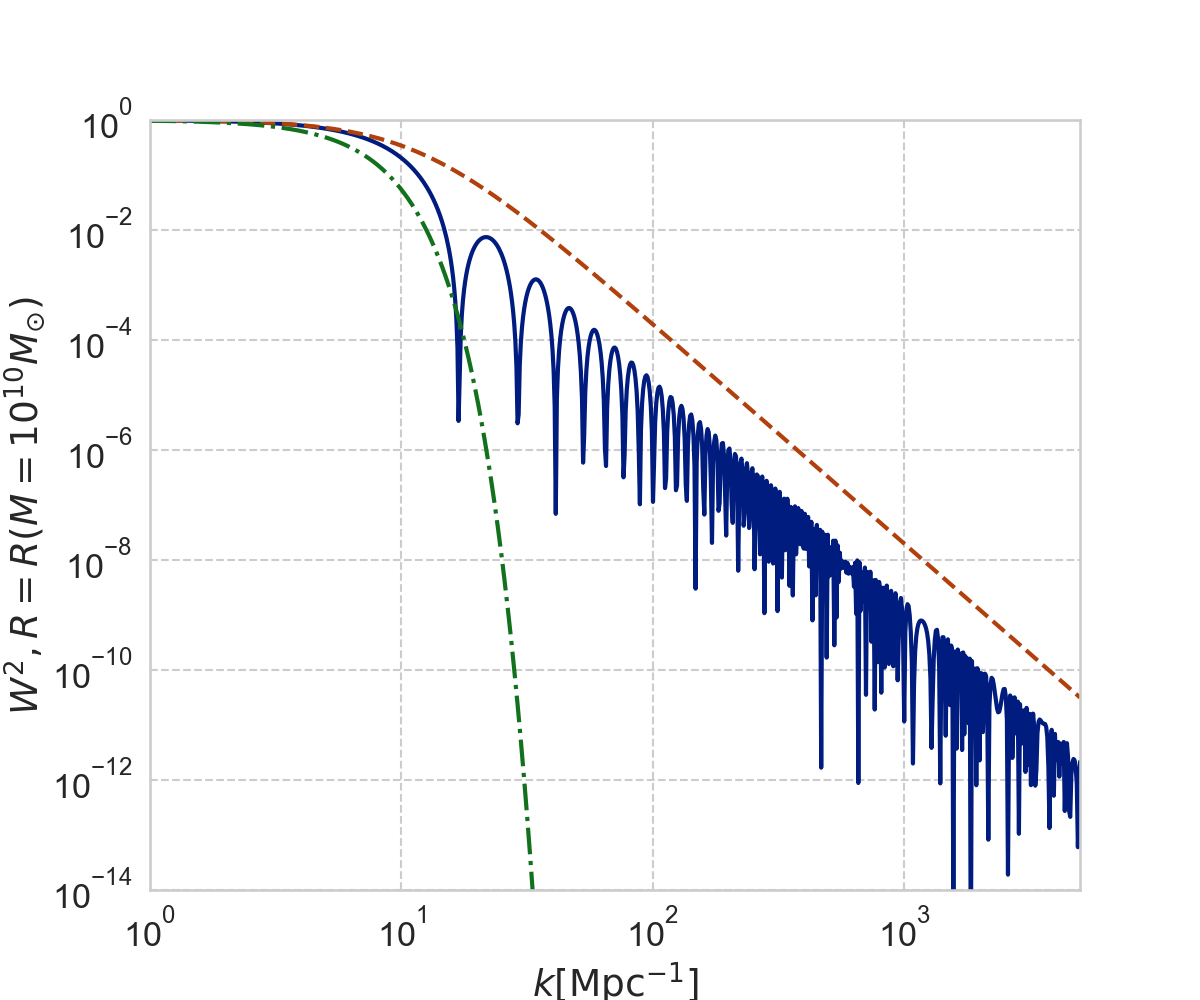
Figure 1: Comparison of window functions $W^{2}$ for the mass scale $M=10^{10}M_{\odot}$. The solid line is the top-hat filter, the dot-dashed line is the Gaussian filter, and the dashed line is the smooth-$k$ filter with $(\beta,c)=(2.0,3.15)$.

In Fig. 1, we show the window functions of top-hat, Gaussian, and smooth-$k$ filter with $(\beta,c)=(2.0,3.15)$. The top-hat filter has oscillating feature around the tail, and the oscillation can make artificial shape in HMF for enhanced PPS models, as has been found in (Yoshiura et al., 2020). The smooth-$k$ filter, on the other hand, has smooth response to the enhancement of PPS at small scales. The Gaussian filter erases the contribution from PPS at small scales, leading to the LFs at $z=6$ roughly 1.3 times smaller than that with the top-hat filter.

II.3 Luminosity Function

Once the halo mass function is calculated, we can evaluate the UV luminosity function as follows Park et al. (2019). We refer the readers to Park et al. (2019) and references therein for the details of the analysis.

First, the stellar mass of a galaxy is converted from halo mass $M_{\rm h}=M$ as

$$M_{*}(M_{\rm h})=f_{\rm star}\left(\frac{\Omega_{b}}{\Omega_{m}}\right)M_{\rm h},$$ (28)

where $f_{\rm star}\leq 1$ is the fraction of galactic gas in stars. This fraction is modeled as

$$f_{\rm star}(M_{\rm h})=f_{*,10}\left(\frac{M_{\rm h}}{10^{10}M_{\odot}}\right)^{\alpha_{\rm star}},$$ (29)

where $f_{*,10}$ is fraction of galactic gas in stars for $M_{\rm h}=10^{10}M_{\odot}$ and the power law from is assumed with $\alpha_{\rm star}$ being a power-law index.

Next, the star formation rate (SFR) is assumed as

$$\dot{M}_{*}(M_{\rm h},z)=\frac{M_{*}(M_{h})}{t_{\rm star}H^{-1}(z)},$$ (30)

where $t_{\rm star}$ controls the star formation rate in unit of Hubble time. The range is restricted to $0<t_{\rm star}<1$. The SFR is related to the rest-frame UV luminosity, which is written as

$$\dot{M}_{*}(M_{\rm h},z)=\mathscr{K}_{\rm UV}\times L_{\rm UV},$$ (31)

where $\mathscr{K}_{\rm UV}=1.15\times 10^{-28}\rm M_{\odot}yr^{-1}/ergs\,s^{-1}\,Hz^{-1}$ Sun and Furlanetto (2016). The UV luminosity is converted to UV magnitude using the AB magnitude relation Oke and Gunn (1983),

$$\log_{10}\left(\frac{L_{\rm UV}}{\rm ergs^{-1}Hz^{-1}}\right)=0.4\times(51.63-M_{\rm UV}).$$ (32)

The SFR in a small mass halo might be suppressed by feedback, which is modeled as

$$f_{\rm duty}(M_{\rm h})=\exp\left(-\frac{M_{\rm turn}}{M_{\rm h}}\right),$$ (33)

where $M_{\rm turn}$ is the mass threshold defined such that a halo with the mass below $M_{\rm turn}$ cannot form stars efficiently.

Combining these models, the UV luminosity function is given by

$$\phi(M_{\rm UV})=f_{\rm duty}\frac{dn}{dM_{\rm h}}\left|\frac{dM_{\rm h}}{dM_{\rm UV}}\right|,$$ (34)

where $M_{\rm UV}$ is the UV magnitude which is related to the UV luminosity as given by Eq. (32).

In addition to the UV LFs, we can also utilize the stellar to halo mass ratio (SHMR) at high redshifts, which has been reported in Harikane et al. (2016). We also include this observation to constrain the astrophysical parameters.

II.4 MCMC analysis and Likelihood

Although our primary purpose is to derive constraints on PPS, we also need to take account of astrophysical parameters since they also affect the UV LFs. We thus perform a Markov Chain Monte Carlo (MCMC) analysis to explore the likelihood as a function of many model parameters. Parameters varied in our analysis and their ranges are summarized in Table 1. Since astrophysical parameters such as $f_{*,10}$, $\alpha_{\rm star}$, $M_{\rm turn}$, and $t_{\rm star}$ can evolve in time, to be conservative, we treat these astrophysical parameters independently for 5 different redshift bins. Hence we vary 20 parameters in total for astrophysical ones. Besides these parameters, there are also several PPS parameters, where the total number of the model parameters depends on the parametrization. The MCMC analysis is performed using the public code emcee Foreman-Mackey et al. (2013). Our criterion for the convergence of the chain is based on the integrated auto-correlation time $\tau$ Goodman and Weare (2010). We accept chain longer than 50$\tau$ and check the convergence such that the value of $\tau$ is almost unchanged even if we increase the number of samples as suggested in Foreman-Mackey et al. (2013).

Table 1: Parameters and their prior ranges in our MCMC analyais. We assume a flat prior within the range for all parameters.

param	min	max	Prior
$f_{*,10}~{}(z=6,7,8,9,10)$	0.001	1.0	log
$\alpha_{\rm star}~{}(z=6,7,8,9,10)$	-0.5	1.0	linear
$M_{\rm turn}~{}(z=6,7,8,9,10)$	$10^{7}M_{\odot}$	$10^{10}M_{\odot}$	log
$t_{\rm star}~{}(z=6,7,8,9,10)$	0.0	1.0	linear
$n_{s}$	0.0	2.0	linear
$\alpha_{s}$	-1	1	linear
$\beta_{s}$	-1	1	linear
$p_{1}$	$10^{-5}$	$10^{8}$	log
$q_{1}$	$10^{-5}$	$10^{8}$	log
$q_{2}$	$10^{-5}$	$10^{8}$	log
$q_{3}$	$10^{-5}$	$10^{8}$	log
$r_{1}$	$10^{-5}$	$10^{8}$	log
$k_{1}$	10.0	$10^{4}$	log

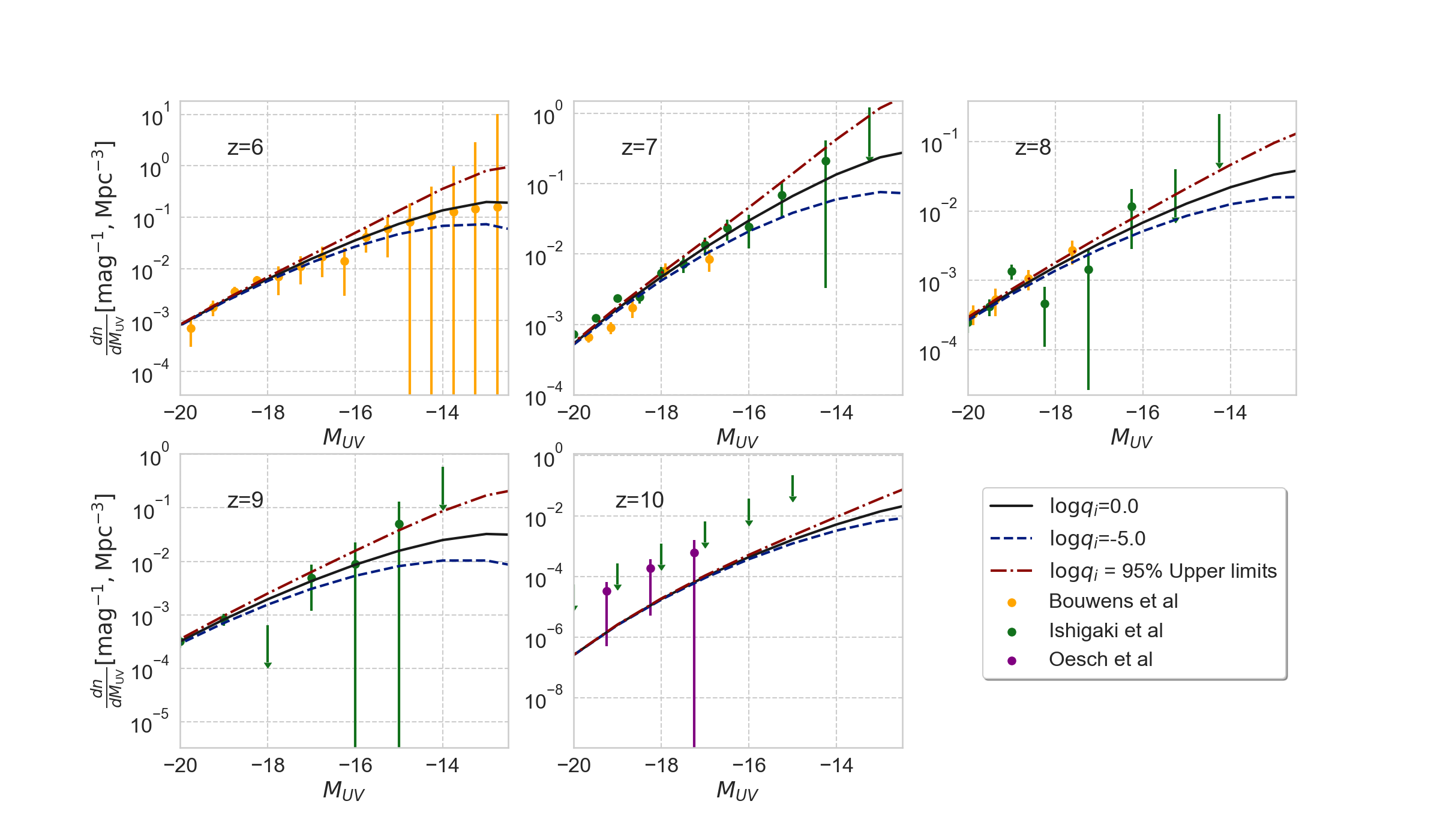
Figure 2: LFs adopted in our analysis. We use those at $z=6$ Bouwens et al. (2017), $z=7$ Bouwens et al. (2017); Ishigaki et al. (2018), $z=8$ Ishigaki et al. (2018), $z=9$ Ishigaki et al. (2018) and $z=10$ Oesch et al. (2018); Ishigaki et al. (2018). Solid, dashed and dot-dashed lines are the LFs for Parametrization III with $\log q_{i}=0$, $\log q_{i}=-5$, and $q_{i}$ values of 95% upper limit for all $i$. For astrophysical parameters, we use the best-fit parameters obtained in the MCMC for Parametrization III.

In our MCMC analysis, the likilihood of each model is evaluated by comparing the model predcited UV LFs at high redshifts $z=6-10$ with those derived from Hubble Frontier Fields data, which is depicted in Fig. 2. More specifically, we assume the following log likelihood for the LFs

$$\ln\mathcal{L}_{\rm LF1}=-\frac{1}{2}\sum_{i}{\frac{(y_{i}-m_{i})^{2}}{\sigma_{i}^{2}}},$$ (35)

where $y_{i}$ is the observed UV LF, $m_{i}$ is the LF calculated based the formalism given in the previous section for a given PPS Parametrization and model parameters, and $\sigma_{i}$ is the error of the observation. The label $i$ refers to each data depicted in Fig. 2. For simplicity, if the asymmetric error is given, we use its averaged value.

When only an upper limit is given in the observed LFs data, the log likelihood is calculated by assuming a Poisson distribution with sample 0 as

$$\ln\mathcal{L}_{\rm LF2}=-\sum_{i}\frac{m_{i}}{(y_{i}/1.15)},$$ (36)

where 1.15 indicates the expected number of galaxies in the bin corresponding to 1$\sigma$ upper limit assuming the Poisson statistics.

The parameters can be constrained using the LFs for each redshift and combining all redshift data. We give our main results from the combination of all redshift data in the next section. Note that the LF of bright galaxies can be suppressed by AGN feedback which is not considered in this model, and therefore we use the LF only at $M_{\rm UV}>-20$, which is the same treatment as in Park et al. (2019).

Based on Harikane et al. (2016), we can also utilize the observed stellar to halo mass ratio (SHMR) to improve constraints. The SHMR is derived from clustering analysis using Hubble deep image and Subaru Hyper Suprime-Cam data. Its likelihood is calculated as

$$\ln\mathcal{L}_{\rm SHMR}=-\frac{1}{2}\sum_{i}\frac{(M_{{\rm halo},i}(M_{\rm UV})-M_{{\rm halo},i,{\rm obs}}(M_{\rm UV}))^{2}}{{\sigma_{{\rm SHMR},i}^{2}}},$$

where $M_{\rm halo,obs}$ is the observed halo mass for a given $M_{\rm UV}$ and $\sigma_{\rm SHMR}$ is its error. By adding the data from SHMR, the constraints on the astrophysical parameters are expected to improve. Since the data is provided in the redshift range of $z=4-7$, we use those for $z=6$ in our MCMC analysis. The inclusion of this SHMR data will be discussed in Section IV.2.

Since the form of PPS on large scales has been well constrained by CMB data, in addition to the data from UV LFs and SHMR, we add the likelihood function which describes the constraint on the spectral index $n_{s}$ from Planck, which effectively combine our analysis with large scale observations of CMB, considering the fact that cosmological parameter sets that are tightly constrained by CMB observations are fixed in our analysis. This can be done by adding the likelihood function for $n_{s}$

$$\ln\mathcal{L}_{\rm Planck}=-\frac{1}{2}\frac{(n_{s}-n_{s(\rm planck)})^{2}}{\sigma^{2}_{n_{s}}},$$ (38)

where we take $n_{s\rm(Planck)}=0.9665$ and $\sigma_{n_{s}}=0.0038$ Akrami et al. (2018).

The total likelihood function is given by the sum of $\ln{\cal L}$ discussed above as

$$\ln{\cal L}_{\rm total}=\ln\mathcal{L}_{\rm LF1}+\ln\mathcal{L}_{\rm LF2}+\ln\mathcal{L}_{\rm SHMR}+\ln\mathcal{L}_{\rm Planck},$$ (39)

with which we investigate constraints on the PPS parameters as well as the astrophysical ones for each redshift.

III Results

Now we present our constraints on the PPS for each Parametrization. We here focus only on key results. The full MCMC corner plots are shown in Appendix B. We also discuss the effect of the stellar to halo mass ratio on the constraints. Although the main purpose of this paper is to derive constraints on the PPS, we also investigate how the cosmological assumption such as the form of PPS affects constraints on astrophysical parameters.

III.1 Constraints on PPS: Parametrization I (runnings)

First we present our results for the case of Parametrization I where the PPS is characterized by the spectral index $n_{s}$, the running $\alpha_{s}$, and the running of the running $\beta_{s}$.

Constraints obtained from the UV LFs and assuming the top-hat filter are

$$n_{s}=0.967_{-0.004}^{+0.003},$$

$$\alpha_{s}=0.050_{-0.090}^{+0.070},$$

$$\beta_{s}=-0.063_{-0.046}^{+0.061}.$$ (40)

The corner plot is shown in Fig. 3. When we adopt the smooth-$k$ filter, constraints on these parameters are given as

$$n_{s}=0.967_{-0.004}^{+0.003},$$

$$\alpha_{s}=0.046_{-0.099}^{+0.077},$$

$$\beta_{s}=-0.057_{-0.049}^{+0.062}.$$ (41)

The constraints above can be compared with the ones from Planck 2018 (Eqs. (16)-(18) in Akrami et al. (2018)):

$$n_{s}=0.9625\pm 0.0048,$$

$$\alpha_{s}=0.002\pm{0.010},$$

$$\beta_{s}=0.010\pm{0.013}.$$ (42)

Our constraints from the UV LFs are consistent with those from Planck. The LF at $z=6$ assuming the mean values given in Eq. (III.1) are shown in Fig. 4. For reference, we also plot the cases with $(n_{s},\alpha_{s},\beta_{s})=(0.97,0.2,0.0)$, and $(n_{s},\alpha_{s},\beta_{s})=(0.97,0.0,-0.1)$. From Fig. 4, one can see that these two cases are completely deviated from the data. Indeed these two models are excluded at 95 % CL as shown in Fig. 3.

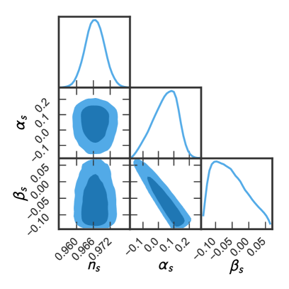
Figure 3: Constraints on $n_{s}$, $\alpha_{s}$, and $\beta_{s}$ for Parametrization I. 68 % and 95% allowed regions are depicted as dark and light blue, respectively. Astrophysical parameters are marginalized. Here the top-hat filter is assumed.

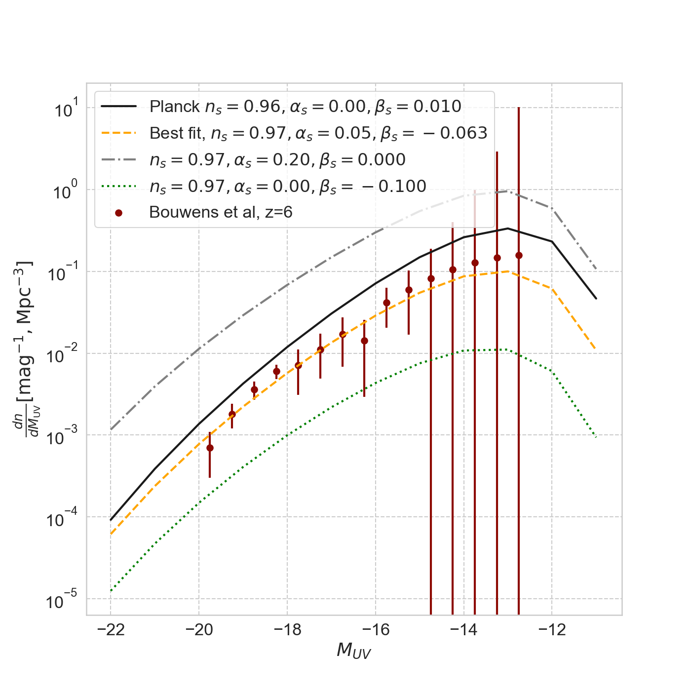
Figure 4: Comparison of the observed and model predicted LFs at $z=6$ for Parametrization I. Solid and dashed lines are the LFs with best-fit running parameters from Planck and the best fit value of our results with the top-hat filter (Eq. (III.1)), respectively. For reference, two extreme models are shown as dot-dashed line ($n_{s}=0.97$, $\alpha_{s}=0.2$, and $\beta_{s}=0.0$) and dotted line ($n_{s}=0.97$, $\alpha_{s}=0.0$, and $\beta_{s}=-0.1$). Astrophysical parameters are taken to be the best-fit values, $\log f_{*,10}=-0.91$, $\alpha_{\rm star}=0.28$, $\log M_{\rm turn}=8.9$, and $t_{\rm star}=0.55$.

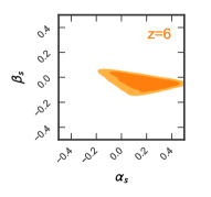
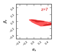
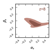
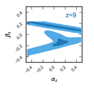
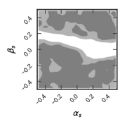
Figure 5: These panels show constraints on $\alpha_{s}$ and $\beta_{s}$ from the UV LFs at $z=6$, 7, 8, 9, and 10 from left to right. 68 % and 95% allowed regions are depicted as dark and light colors, respectively. These constraints are derived by performing the MCMC analysis only at each redshift.

Fig. 5 shows running parameters constrained by using LFs for each redshift. These panels indicate that the constraints shown in Fig. 3 are dominated by those from the LFs at $z\leq 8$. For example, cases with $(n_{s},\alpha_{s},\beta_{s})=(0.97,0.2,0.0)$, and $(n_{s},\alpha_{s},\beta_{s})=(0.97,0.0,-0.1)$ are ruled out because these models enhance and reduce the LFs overall as shown in Fig. 4. This is due to the fact that the running parameters change the overall PPS amplitude around the relevant scale ($1<k<10\rm Mpc^{-1}$), and hence the enhancement or the suppression of the LFs is independent of the galaxy magnitude $M_{\rm UV}$.

III.2 Constraints on PPS: Parametrization II
(step function-like PPS)

Next we show our results for the case of Parametrization II. The PPS is described as a step function-like form at $k>10\rm Mpc^{-1}$. As in Parametrization I, we use the LFs at all redshift and the prior on the $n_{s}$ to constrain 22 free parameters. The constraint on the $p_{1}$ is shown in Fig. 6. We find that $p_{1}$ is consistent with 0 with the 95% upper limit of

$$\log p_{1}<0.10.$$ (43)

The constraint is stronger than previous constraints on the PPS (e.g. Fig. 6 in Bringmann et al. (2012)). The UV LFs cannot place the lower limit on $p_{1}$ because ${\cal P_{\zeta}}(k)$ at large scales dominates the mass variance and hence, even if small scale amplitude gets significantly suppressed, the LFs do not decrease even for extremely low values $p_{1}$.

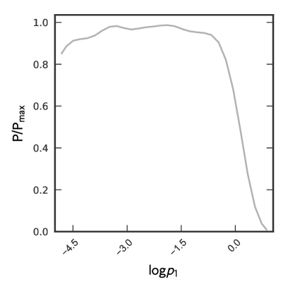
Figure 6: The posterior distribution of $p_{1}$ for Parametrization II with other parameters marginalized. This constraint is derived using all the UV LFs.

In the same way as in Parametrization I, in order to clarify LFs from which redshift dominate the constraints, we show constraints on $p_{1}$ and $n_{s}$ from the LFs at each redshift in Fig. 7. The panels show that the constraints are dominated by those from the UV LF at $z=9$. Note that extremely large $p_{1}$ is allowed at $z=6$ and $z=8$ if $f_{\rm star}$ is sufficiently small. In this case, other astrophysical parameters take values of $\log f_{*,10}\approx-2.5$ and $\alpha_{\rm star}=0.0$. However, such models are rejected because the halo mass function becomes too high even at $z\geq 9$.

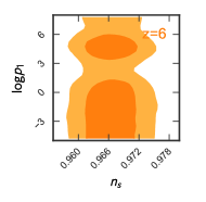
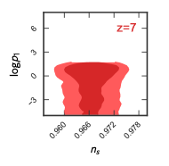
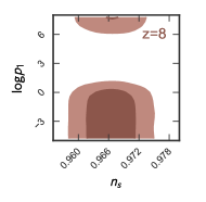
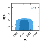
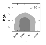
Figure 7: Same as Fig. 5, but for constraints on $n_{s}$ and $p_{1}$ for Parametrization II.

III.3 Constraints on PPS: Parametrization III (binned PPS)

For the case of Parametrization III, the PPS is described by a binned step functions-like form. The one-dimensional posterior distributions for $q_{1}$, $q_{2}$, and $q_{3}$, which characterize the amplitude of each bin, are shown in Fig. 8. For the top-hat filter, 95 % upper bounds are obtained as

$$\log q_{1}<0.2,$$

$$\log q_{2}<3.2,$$

$$\log q_{3}<6.9.$$ (44)

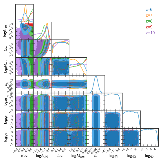
Figure 21: Same as Fig. 19, but for Parametrization III. This result is discussed in Sec. III.3, and best fit astrophysical parameters and upper limits on $q_{i}$ ($i$=1, 2, 3) are listed in Table 2 and 3 respectively.

We note that our constraint on PPS at $k<100\rm Mpc^{-1}$ is stronger than those obtained in previous work. Constraints on astrophysical parameters are listed in Table. 2 and those on PPS parameters are given in Table 3. The full corner plot is shown in Appendix B (Fig. 21).

Examples of LFs are shown in Fig. 2, where we compare the LFs with $\log q_{1,2,3}=0$, $\log q_{1,2,3}=-5$ and a model with 95 % upper limit of $q_{1,2,3}$. The figure shows that the small scale PPS controls the faint end of LFs. Thus, future improved constraints on the faint end of LFs have a potential to tighten constraints on PPS at small scales.

Interestingly, the best-fit value of $\alpha_{\rm star}$ depends on redshift, which hints the redshift evolution of these parameters. Therefore the evolution of these astrophysics parameters should be taken into account in future parameter estimations including those via 21cm line. However, the understanding the evolution of such astrophysical parameters is beyond the scope of this work.

Table 2: Summary of constraints on astrophysical parameters obtained from MCMC analysis using UV LFs from all redshifts and the prior on the $n_{s}$ from Planck for Parametrization III. Here we assume the smooth-$k$ filter.

	$z=6$	$z=7$	$z=8$	$z=9$	$z=10$
$\alpha_{\rm star}$	$0.301_{-0.154}^{0.188}$	$0.342_{-0.080}^{0.097}$	$0.834_{-0.167}^{0.115}$	$0.788_{-0.221}^{0.149}$	$0.302_{-0.499}^{0.459}$
$\log f_{*,10}$	$-1.204_{-0.419}^{0.238}$	$-1.156_{-0.354}^{0.200}$	$-1.531_{-0.410}^{0.226}$	$-1.138_{-0.435}^{0.247}$	$-2.129_{-0.567}^{0.545}$
$t_{\rm star}$	$0.522_{-0.320}^{0.317}$	$0.547_{-0.305}^{0.300}$	$0.525_{-0.319}^{0.313}$	$0.512_{-0.323}^{0.321}$	$0.580_{-0.323}^{0.285}$
$\log M_{\rm turn}$	$8.965_{-0.642}^{0.605}$	$8.673_{-0.453}^{0.521}$	$9.203_{-0.787}^{0.589}$	$9.175_{-0.763}^{0.601}$	$9.022_{-0.680}^{0.663}$

Table 3: Summary of constraints on PPS parameters for Parametrization III obtained from the MCMC analysis using UV LFs from all redshifts. Here we present the results for each filter. Since the posterior distributions of $q_{i}$ is not Gaussian for all $i$, we only show the 95% upper limit $q_{i}^{\rm up}$. Note that we do not obtain an upper bound for $q_{2}$ and $q_{3}$ when top-hat and Gaussian filters are adopted.

	Smooth-$k$	Top-hat	Gaussian
$\log q_{1}^{up}$	0.15	0.57	0.81
$\log q_{2}^{up}$	3.18	4.42	-
$\log q_{3}^{up}$	6.83	-	-

The constraints depend on the choice of the filter. In Fig. 8, we compare the constraints for various filters. The result indicates that the constraints are tighter when the smooth-$k$ filter is assumed. This is due to the fact that the smooth-$k$ filter allows small scale PPS to contribute to the mass variance as shown in Fig. 1. However, even in the case of the top-hat filter, the constraint on the PPS at $k<100~{}\rm Mpc^{-1}$ is tighter than in previous work Bringmann et al. (2012) (in our case ${\cal P}_{\zeta}(10<k<100~{}{\rm Mpc}^{-1})<{\cal O}(10^{-8})$). Note that the top-hat filter can show artificial features in the LFs for models with extremely large $q_{i}$ ($i$=1, 2, 3) as shown in Yoshiura et al. (2020). In contrast, since the Gaussian filter erases the small scale power completely, the constraint is weak. The UV LFs cannot constrain $q_{2}$ and $q_{3}$, but the $q_{1}$ should be less than ${\cal O}(10)$, i.e., ${\cal P}_{\zeta}(10<k<100~{}{\rm Mpc}^{-1})<{\cal O}(10^{-8})$. We again caution that the appropriate filter should ultimately be chosen by comparing the mass function with $N$-body simulation results with such an enhanced PPS model.

The constrained astrophysical parameter for each filter are consistent within 1$\sigma$ error while the best fit value of $\alpha_{\rm star}$ and $f_{*,10}$ slightly depend also on the choice of the filter (see Fig. 24 in Appendix B). We will discuss the effect of the cosmological assumption on the astrophysical parameters in later section.

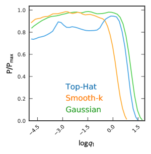
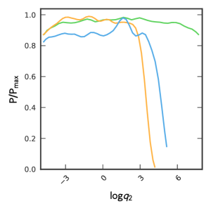
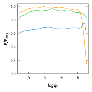
Figure 8: One-dimensional posterior distributions for $\log q_{1}$, $\log q_{2}$, and $q_{3}$ for Parametrization III. Blue, orange, and green lines are the result with top-hat, smooth-$k$, and Gaussian filters, respectively.

III.4 Constraints on PPS: Parametrization IV (scale dependent step function-like PPS)

We show the result for Parametrization IV in Fig. 9. This parametrization describes a step function-like form with an arbitrary transition scale. In this case, the upper limit on the PPS can be estimated at various scales. In Fig. 9, the corner plot of $r_{1}$ and $k_{1}$ shows that the larger $k_{1}$ is, the larger fluctuation is allowed. This figure also indicates that upper limits on the PPS are placed for a wide range of scales.

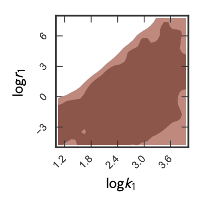
Figure 9: Constraints on $r_{1}$ and $k_{1}$ for Parametrization IV from the MCMC analysis using UV LFs from all redshifts. The smooth-$k$ filter is adopted in this figure. 68 % and 95% allowed regions are depicted as dark and light colors, respectively.

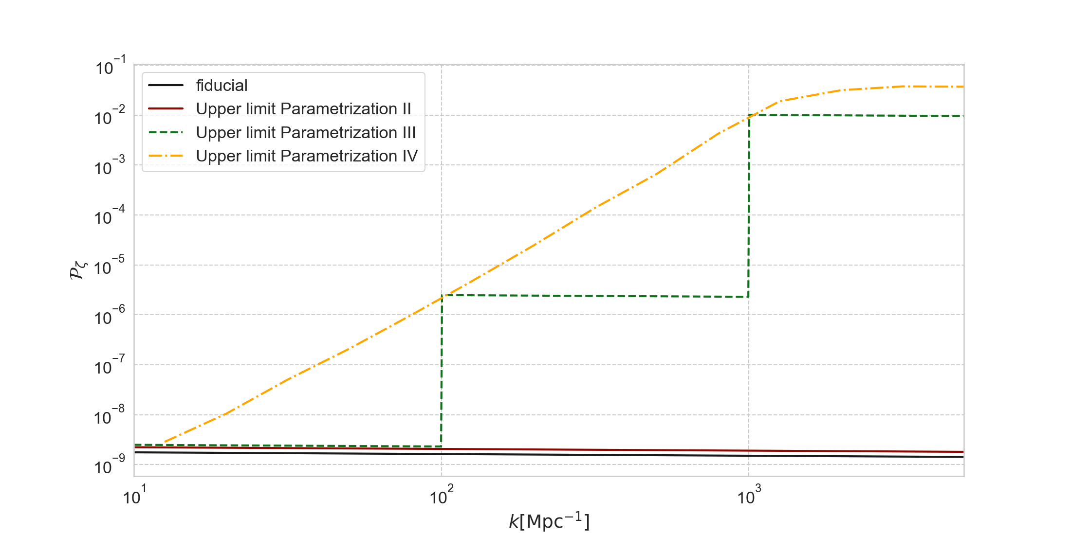
Figure 10: Upper limits on PPS for various parmetrizations for the smooth-$k$ filter. Upper solid, dashed, and dot-dashed lines show the 95% upper bounds for the parametrization II, III, and IV, respectively. We plot PPS with $\log q_{i=1,2,3}=0$ as fiducial.

III.5 Constraints on PPS: Parametrization V (power-law PPS)

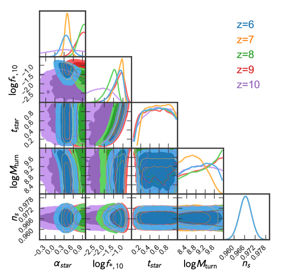
Figure 23: Same as Fig. 19, but for Parametrization V. This result is discussed in Sec. III.5.

In Parametrization V, only $n_{s}$ is allowed to vary. The $n_{s}$ is severely constrained by the Planck. Thus, we can obtain best fit astrophysical parameters without PPS uncertainty. The constraints on the astrophysical parameters are fairly consistent with the values shown in Park et al. (2019). The full result is shown in Fig. 23 of Appendix B.

III.6 Summary of constraints on PPS

In Fig. 10, we summarize the 95% upper bounds obtained in Parametrization II, III, and IV for the smooth-$k$ filter. For Parametrization IV, we assort MCMC samples into several $k$-bins and calculate 95% upper limits from the samples in each $k$-bin, which almost corresponds to the upper bound in Fig. 9. We find that our results for Parametrization III and IV are reasonably well consistent with each other. It is also found that the analysis for Parametrization II severely overestimate the upper limits on PPS at very small scales.

IV Discussions

IV.1 Interpretation of the constraints from UV Magnitude

In order to interpret the constraints, it is useful to see which scale $k$ is responsible for a halo with $M_{\rm halo}$ and UV magnitude $M_{\rm UV}$. $M_{\rm halo}$ and $k$ are related via Eqs. (18), (22), and (27) for top-hat, Gaussian, and smooth-$k$ filters, respectively. $M_{\rm UV}$ is given for a fixed $k$ from the formulas given in Section II.2. In the upper panel of Fig. 11, we show the $M_{\rm halo}$-$k$ relation, which indicates that the smooth-$k$ filter allows us to explore the PPS on smaller scales than in other filters. We also show the $M_{\rm UV}$-$k$ relation in the bottom panel of Fig. 11 with the best-fit astrophysical parameters for each filter derived in Parametrization III. This panel indicates that observations of faint-end galaxies down to $M_{\rm UV}\approx-14$ can probe the scales of $k\approx 100\rm Mpc^{-1}$ at $z=6$. This is why the UV LFs can constrain $q_{1}$ and $q_{2}$ for Parametrization III.

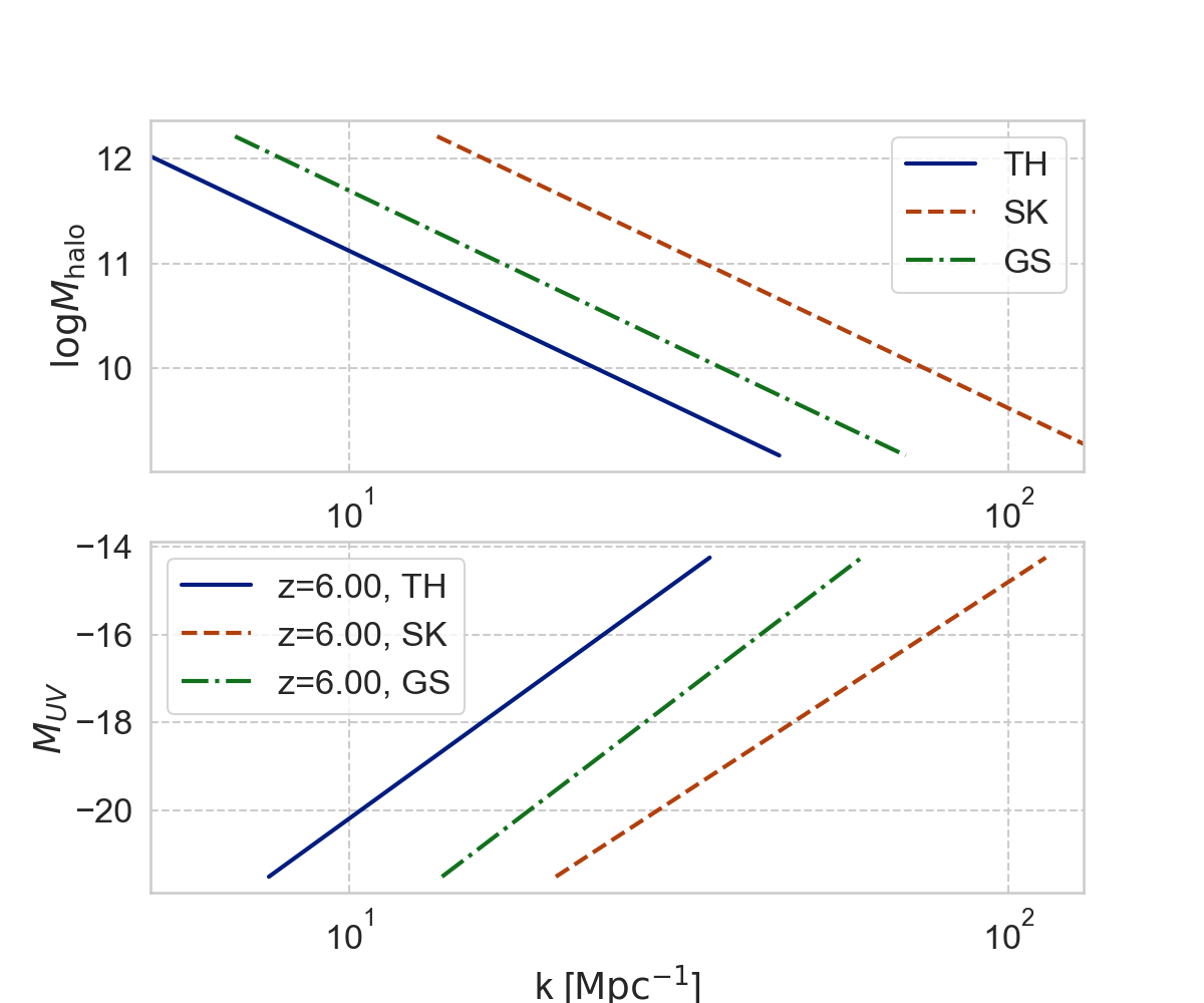
Figure 11: Upper: Relation between halo mass $M_{\rm halo}$ and the wavenumber $k$ for each filter at $z=6$. Lower: Relation between galaxy UV magnitude $M_{\rm UV}$ and $k$ for each filter at $z=6$ assuming the best-fit astrophysical parameters for Parametrization III.

Not only the mass scale but also the shape of the filter as a function of $k$ is crucial for understanding the constraints. Fig. 1 indicates that the smooth-$k$ filter has a strong response to small scales, and this is why the constraint with the smooth-$k$ filter is tighter than in other ones. The Gaussian filter, on the other hand, does not pick up fluctuations on small scales. Thus, the PPS at $k>20\,\rm Mpc^{-1}$ cannot be constrained with the Gaussian filter.

The integral of Eq. (LABEL:eq:dlnsigmadlnm) controls the contribution to the mass function from fluctuations at small scales. Thus, a cumulative contribution of the integral up to $k$ mode is useful to estimate the contribution from particular mass scales. Fig. 12 shows the ratio of cumulative contribution for PPS with Parametrization III against to a fiducial model with $q_{1}=q_{2}=q_{3}=1$. In the figure, we show the cumulative contribution for a galaxy with $M_{\rm UV}=-15$ which corresponds to $M=10^{9.6}M_{\odot}$. This figure shows that the smooth-$k$ filter picks up more power from the enhanced PPS on small scales.

For a model with $q_{1}=10$ ($q_{2}=10^{4}$), the total contribution from the smooth-$k$ filter in the range of $10~{}{\rm Mpc}^{-1}<k<100~{}{\rm Mpc}^{-1}$ ($100~{}{\rm Mpc}^{-1}<k<1000~{}{\rm Mpc}^{-1}$) is 4.5 (4.0) times larger than the fiducial model. On the other hand, in the case of the top-hat filter, the enhancement of the total contribution is smaller than in the smooth-$k$ filter. This is why the top-hat filter gives weaker upper limits on $q_{i}$ ($i$=1, 2, 3) compared to those for the smooth-$k$filter.

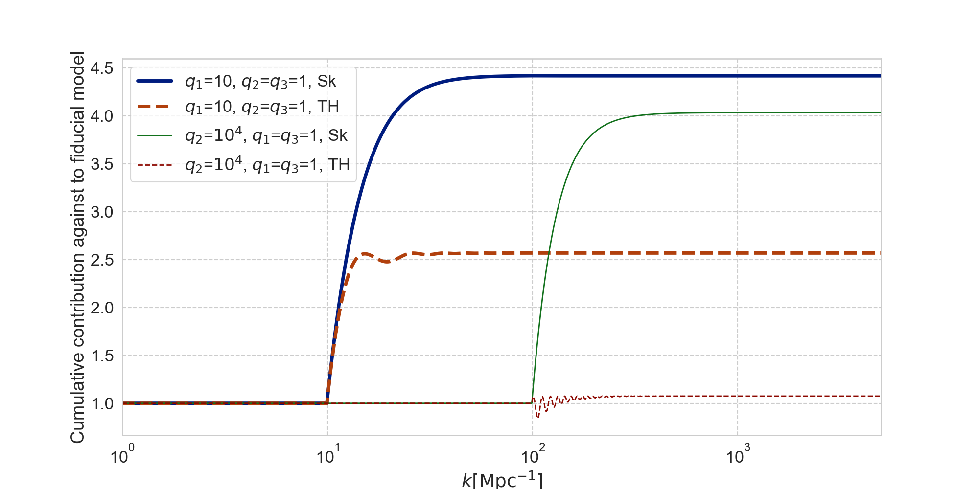
Figure 12: Cumulative value of Eq. (LABEL:eq:dlnsigmadlnm) for enhanced PPS models. For comparison, we plot the ratio against to $p_{1}=p_{2}=p_{3}=1$ model. Dashed lines show the result with the top-hat filter, and solid lines are the result with the smooth-$k$ filter.

IV.2 Impact of stellar to halo mass ratio

We have also included the data of the stellar to halo mass ratio (SHMR) Harikane et al. (2016) in our MCMC analysis to constrain the parameters. Although the SHMR relation is constrained only at the bright end of the LFs ($M_{\rm UV}\approx-20$), it still helps improve constraints on PPS by constraining the astrophysical parameters. A caveat is that constraints on SHMR from the clustering analysis in principle depend on PPS. However, the SHMR is mainly constrained from the so-called 2-halo term of the galaxy auto correlation function at $\theta>20^{\prime\prime}$, which corresponds to $k<8\,\rm Mpc^{-1}$ at $z=6$. This $k$ range is smaller than that of our interest, and therefore for simplicity we assume that the constraints on the SHMR in Harikane et al. (2016) does not depend on PPS and thus do not change throughout the MCMC analysis.

To check this point explicitly, in Fig. 13 we show results of MCMC using the UV LF at $z=6$ and/or the SHMR with the top-hat filter for PPS with $p_{1}$ (Parametrization II). In Table 4, we list constraints on the astrophysical parameters as well as on the PPS parameter. We find that the best-fit value of $\alpha_{\rm star}$ varies somewhat by adding the SHMR data. In order to understand this result, we plot the SHMR and the UV LF at $z=6$ using the best-fit parameters in Fig. 14. The left panel indicates that, in order to reproduce the observed SHMR, star formation rate (SFR) in halo of $M_{h}\approx 10^{11.5}M_{\odot}$ has to be suppressed. Here, the SHMR is described as $L_{\rm UV}\propto f_{*,10}M^{\alpha_{\rm star}+1}_{h}$. However, $f_{*,10}$ is required to be $\approx$ 0.1 for reproducing the LF at $M_{\rm UV}\approx-17$. Thus, the slope $\alpha_{\rm star}$ becomes flatter to maintain the UV LF and to satisfy the constraints on the UV LF and the SHMR simultaneously. Since $\alpha_{\rm star}$ becomes flatter, the lower halo mass scales can be explored at faint-end of LFs. Thus, the constraints on the astrophysical parameters and $p_{1}$ become slightly tighter.

By adding the SHMR to the MCMC analysis, the constraints on $\alpha_{\rm star}$ becomes tighter. Thus, the SHMR is useful to remove the degeneracy between $\alpha_{\rm star}$ and the mass dependence of the escape fraction of ionising photons which has been found in Park et al. (2019).

Interestingly, the higher $M_{\rm turn}$ value is preferred to reduce the LFs at $M_{\rm UV}\approx-15$ when we use the UV LF and the SHMR in the MCMC as shown in Fig. 13. This is because the flatter $\alpha_{\rm star}$ increases the UV LF too much at $M_{\rm UV}\approx-15$ since lower mass halos can be responsible for the UV LF.

Table 4: Summary of parameters obtained by MCMC using the UV LF at $z=6$ and/or SHMR.

parameter	LF($z=6$) + SHMR	LF($z=6$)
$\alpha_{\rm star}$	$0.069_{-0.104}^{0.099}$	$0.454_{-0.189}^{0.230}$
$\log f_{*,10}$	$-1.113_{-0.460}^{0.245}$	$-1.192_{-0.456}^{0.249}$
$t_{\rm star}$	$0.510_{-0.333}^{0.327}$	$0.519_{-0.337}^{0.324}$
$\log M_{\rm turn}$	$9.554_{-0.762}^{0.306}$	$9.053_{-0.706}^{0.605}$
$n_{s}$	$0.968_{-0.004}^{0.003}$	$0.966_{-0.003}^{0.004}$
$\log p_{1}^{up}$	0.71	1.54

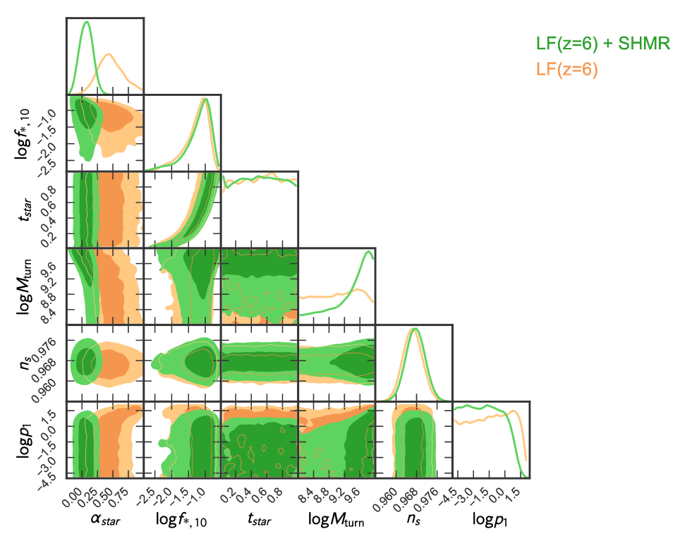
Figure 13: Result for the MCMC analysis for Parametrization II using only the UV LF at $z=6$ (orange) and both the UV LF and SHMR at $z=6$ (green).

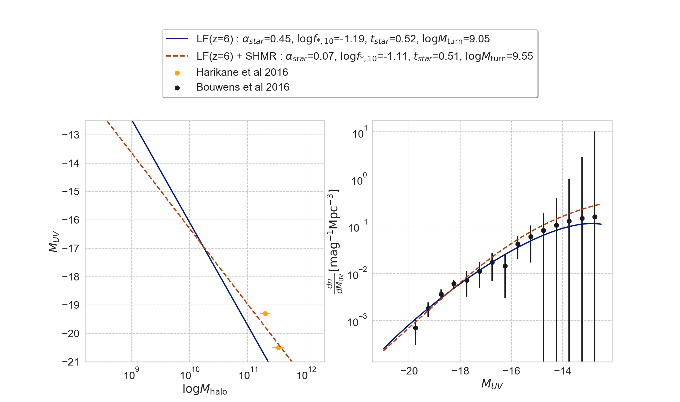
Figure 14: Left: Relation between $M_{\rm UV}$ and $M_{\rm halo}$ at $z=6$. The observational constraints from Harikane et al. (2016) are compared with best-fit models from the UV LF at $z=6$ only (solid) and from both UV LF and SHMR (dashed). See Tabel 4 for the best-fit parameters. Right: Comparison of the observed UV LF at $z=6$ from Bouwens et al. (2017) with best-fitting models also shown in the left panel. Here we fix $p_{1}=1$.

IV.3 Effects of cosmological assumptions on astrophysical parameters

Since we allow the form of PPS to vary especially on small scales, constraints on astrophysical parameters may be affected due to the degeneracy with the PPS parameters. Here we discuss how the astrophysical parameter estimation depends on the assumption on cosmology.

In Fig. 15, we show the one-dimensional posterior distributions of $\alpha_{\rm star}$ and $f_{*,10}$ which are obtained using UV LFs from all redshifts to compare the results for all the parametrizations with the smooth-$k$ filter.

For Parametrization I, $\alpha_{\rm star}$ and $f_{*,10}$ show weak correlations with $\alpha_{s}$ and $\beta_{s}$ as shown in Fig. 16. Due to the degeneracy, the constraints on the astrophysical parameters are slightly loosen compared to the result of Parametrization V.

On the other hand, the results of the other parametrizations of the PPS do not show any deviations from that of Parametrization V, which has the standard simple power-law form when we include the data from all redshifts. However, when we perform MCMC using LFs only at $z=7$, a clear degeneracy is found between $p_{1}$, $f_{*,10}$, and $\alpha_{\rm star}$ as shown in Fig. 17. Since large $p_{1}$ increases the halo mass function at small mass scales, low $f_{\rm star}$ with positive $\alpha_{\rm star}$ and lower $f_{\rm*,10}$ can somewhat compensate the enhancement due to PPS. However this degeneracy does not affect Fig. 15 since the model with higher $p_{1}$ value is rejected by combining the UV LFs from other redshifts.

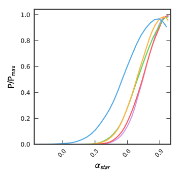
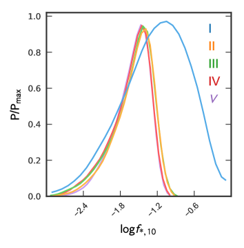
Figure 15: Comparison of one-dimensional posterior distributions of $\alpha_{\rm star}$ (left) and $f_{*,10}$ (right) at $z=8$ with different parametrizations of PPS. We show results of the MCMC analysis using the UV LFs from all redshifts assuming the smooth-$k$ filter.

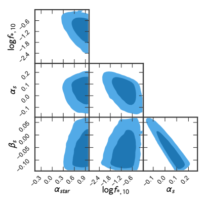
Figure 16: Corner plot for Parametrization I. We show constraintns on the running parameters and astrophysical parameters $\alpha_{\rm star}$ and $f_{*,10}$) at $z=8$.

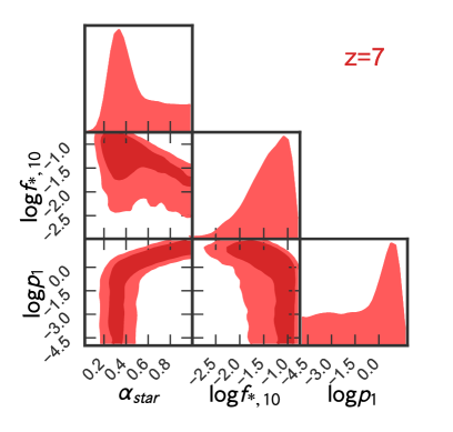
Figure 17: Corner plot obtained by the MCMC analysis using UV LF at $z=7$ for Parametrization II.

The redshift evolution of astrophysical parameter can also depend on the parametrization. For Parametrization II, III, and IV, the parameter evolution is same as that for Parametrization V. While the constraints become weak for Parametrization I (which is characterized by the runnings), the trend of the redshift evolution does not change. This can be seen in the full result of the MCMC analysis for each Parametrization shown in Appendix B.

The best-fit values of astrophysical parameter $\alpha_{\rm star}$ and $f_{*,10}$ slightly depend on the choice of the filter as shown in Fig. 24 , while the values for each filter are consistent with each other within 1 $\sigma$ error. For example, the Gaussian filter underestimate the halo mass function compared to other filters because the Gaussian filter erase the small scale contribution to the mass variance. Thus, in order to increase $f_{\rm star}$, the best fit value of $\alpha_{\rm star}$ becomes larger when the Gaussian filter is adopted.

IV.4 Model Uncertainties

In this subsection, we discuss the uncertainties in the model of galaxy. First, dust attenuation should be taken into account carefully even for high redshift LFs. For example, in Shimizu et al. (2014); Clay et al. (2015), using numerical simulation results, they have shown that the LFs at $M_{\rm UV}<-19$ are decreased by the dust attenuation. However, the small scale PPS changes the LFs mainly at $M_{\rm UV}>-16$ as shown in Fig. 2. Thus, the dust effect on the PPS upper limits should be marginal, and thus we ignore the dust attenuation in our LF model.

We adapt a power law form for the stellar to halo mass ratio because the power law model is shown to be reasonable for faint galaxies as indicated in numerical simulations (e.g., Shimizu et al. (2014); Ceverino et al. (2017); Rosdahl et al. (2018); Ma et al. (2018)). Although the model well reproduces the observed LFs, these assumptions on the functional forms might bias the constraints on the PPS if the true functional forms are different from those assumed forms. Possible another choice of the functional form is a double power law form adopted in Tacchella et al. (2018). However, they found the break mass of $M_{\rm halo}\approx 10^{11}M_{\odot}$, below which a single power law form is well consistent with radiation hydrodynamics numerical simulations. Since we use relatively faint galaxies ($M_{\rm UV}>-20$), the assumption of the single power law is consistent with Tacchella et al. (2018). The double power law model may be more appropriate when we use LFs of bright galaxies in the MCMC. We also note that, in Fig.14 of Tacchella et al. (2018), numerical simulation results are not consistent with each other and the result shows that the stellar to halo mass ratio has large variance at small mass scales. Thus, as alternative form, for example, a stochastic implementation of the stellar mass–halo mass relation may be more suitable to predict the UV LF at the faint end. While it would be interesting to compare the results using other forms to describe the LFs more flexibly, we leave it for future work.

Furthermore, modelling of astrophysical effects should involve various uncertanities. For example, internal and external UV backgrounds significantly suppress the star formation in low mass halos corresponding to the very faint end of current observations (e.g., $M_{\rm halo}<10^{9}M_{\odot}$, Hasegawa and Semelin (2013)). In addition to the UV feedback, the relative velocity of baryon and dark matter can suppress the star formation in small mass halos. These effects might be more important if we employ even fainter galaxies in the MCMC. We use an exponential form for the duty cycle to take account of the suppression of star formation in small galaxies due to supernova feedback following Park et al. (2019). The exponential form fits the galaxy evolution in hydrodynamical numerical simulations. Although the model is suggested from numerical simulations and it reproduces the LFs well, there are uncertainties due to the parametrization and other astrophysical effects that might impact on the constraints on the PPS.

The SFR is calculated using Eq. (30), indicating that $f_{*,10}$ and $t_{\rm star}$ are degenerated perfectly. Since we use liner- and log-uniform priors for $t_{\rm star}$ and $f_{*,10}$, respectively, the degeneracy at $t_{\rm star}<0.1$ might not be sampled well in our analysis. The degeneracy can be resolved by adding constrains on the star formation rate and stellar mass relation, the so-called main sequence (MS) relation. In Santini et al. (2017), for example, the MS relation of galaxies at $5<z<6$ has been reported. By comparing their results and Eq. (30), we find that $t_{\rm star}\approx 0.1$ is appropriate. On the other hand, in Bhatawdekar and Conselice (2020), the lower SFR for galaxies at $z>6$ has been reported, which indicates that $t_{\rm star}\approx 0.5$ might be preferred. We emphasize that this degeneracy does not affect our upper limits on PPS since $t_{\rm star}$ and $f_{*,10}$ do not correlate with PPS parameters.

The prior range of parameters can affect the constraints. Although $\alpha_{\rm star}=0.5$ is preferred as shown in Park et al. (2019) and numerical simulations indicate the $\alpha_{\rm star}\approx 1$ (e.g., Ceverino et al. (2017)), the prior range can be extend to $\alpha_{\rm star}>1$. In this case, PPS parameters can be degenerate with $\alpha_{\rm star}$ outside of our prior range at $z=8$ and $z=9$ although the constraints should be dominated by the contribution from LFs at $z=6$ and $z=7$. Thus, by extending the prior range, the constraints might become weaker but this effect should be marginal. The range of the other parameters are well motivated and the effects of the prior range on the constraints should be negligible. The model has no physical meaning for $f_{\rm*,10}>1$, $t_{\rm star}>1$, and $t_{\rm star}<0$. The lower and upper bounds of $M_{\rm turn}$ originate from atomic cooling and the faint end of observed LFs Park et al. (2019).

V Conclusion and Discussions

We have derived constraints on small scale primordial power spectrum (PPS) by using high-redshift galaxy UV luminosity functions. Since the halo mass function at low masses has contribution from small scale PPS, we can constrain PPS at small scales from the observed number density of faint galaxies.

We have employed observed UV LFs at $z=6$–$10$ from Hubble Frontier Fields and performed the MCMC analysis to constrain model parameters. For the assumption of astrophysics, we have followed the model used in Park et al. (2019). We have considered 5 different parametrizations to model PPS at small scales.

We have found that the running parameters $\alpha_{s}$ and $\beta_{s}$ for Parametrization I are constrained by the UV LFs although the constraints are weaker than those obtained by Planck.

We have also considered models with binned PPS at $k>10~{}\rm Mpc^{-1}$ (Parametrization II–IV) assuming the independent amplitude for each bin. For Parametrization III, 95% upper limits are obtained as $\log q_{1}<0.15$ and $\log q_{2}<3.2$. These constraints translate into ${\cal P}_{\zeta}(10<k<100~{}{\rm Mpc}^{-1})<{\cal O}(10^{-8})$ and ${\cal P}_{\zeta}(100<k<1000~{}{\rm Mpc}^{-1})<{\cal O}(10^{-5})$.

Here we compare our constraint with other small scale probes of PPS. Lyman-$\alpha$ forest data constrains PPS as ${\cal P}_{\zeta}\sim(1-3.5)\times 10^{-9}$ at the scale of $k\sim{\cal O}(1)~{}{\rm Mpc}^{-1}$ Bird et al. (2011), which is very severe although the scales probed is relatively limited. Primordial black holes can also constrain the small scale amplitude for a broad range of scale as down to $k\sim{\cal O}(10^{20})~{}{\rm Mpc}^{-1}$, however, its upper bound is ${\cal P}_{\zeta}<{\cal O}(10^{-1})-{\cal O}(10^{-2})$ Josan et al. (2009); Sato-Polito et al. (2019), which is rather weak. CMB spectral $\mu$ distortion can also give a bound on PPS at small scales. From COBE/FIRAS data, one can limit PPS as ${\cal P}_{\zeta}(10<k<10^{4}~{}{\rm Mpc}^{-1})<{\cal O}(10^{-5})$ Chluba et al. (2012, 2019). Ultracompact minihalo (UCMHs) can also put bound on PPS at small scales as ${\cal P}_{\zeta}(10<k<10^{7}~{}{\rm Mpc}^{-1})<{\cal O}(10^{-6})-{\cal O}(10^{-7})$ Bringmann et al. (2012), which is relatively severe although it depends on the nature of dark matter. Compared to these other probes, our constraints from galaxy UV luminosity function can put a severe constraint around the scale of $10<k<1000~{}{\rm Mpc}^{-1}$. Although astrophysics modeling may give some uncertainties to the bound, it would not change the constraints by many orders of magnitude and such uncertainties would be reduced by understanding astrophysical aspects more with other observations, e.g., future 21 cm signal at high redshifts Park et al. (2019). Therefore our method is complimentary to other probes and, for the scales of $10<k<1000~{}{\rm Mpc}^{-1}$, it can serve as a unique probe of PSS on such small scales.

We have also found that the constraints depend on the filter used to calculate the mass variance $\sigma$. Since the appropriate filter for the enhanced PPS model is unknown, we have compared results with smooth-$k$, top-hat, and Gaussian filters to estimate uncertainties associated with the filter. We have found that the constraints on the PPS depend on the response of the filter at small scales. For the top-hat filter, the constraints are loosen slightly compared to the results with the smooth-$k$ filter. For the Gaussian filter, the PPS at small scales cannot contribute to the mass variance, and as a result PPS at $k>100~{}\rm Mpc^{-1}$ cannot be constrained. Even for the Gaussian filter, however, $q_{1}$ is constrained to $q_{1}<10^{1.2}$.

We have also used the observed stellar to halo mass ratio (SHMR) in our MCMC analysis. The constraints from SHMR help tighten constraints on the astrophysical parameters, which lead to improved constraints on the PPS parameters in some cases.

We have also investigated the effects of cosmological assumption on the astrophysical parameters estimation from the UV LFs and found that $\alpha_{\rm star}$ and $f_{*,10}$ can degenerate with the PPS parameters, which indicates that the assumption on cosmology affects the study of astrophysics and vice versa.

Our study shows that astrophysical data such as UV LFs can be a useful probe of cosmology. On the other hand, when one investigates astrophysical aspects, it would also be necessary to take account of the uncertainty of the assumption on cosmological models. Although it looks a bit cumbersome to consider both astrophysical and cosmological aspects, it could also lead to interesting avenue of research ahead of future observations such as James Webb Space Telescope.

Appendix A Mass Variance

Since the amplitude of PPS is fixed and the $n_{s}$ and $q_{i}$ ($i$=1, 2, 3) are parameters used in MCMC, the value of $\sigma_{8}$ might break its constraints. To ensure that our model predicts $\sigma_{8}$ that is consistent with other results, we convert the MCMC samples to $\sigma_{8}$ as shown in Fig. 18. Our result is consistent with e.g., $0.8102\pm 0.0060$ in Akrami et al. (2018) well within 1$\sigma$ error.

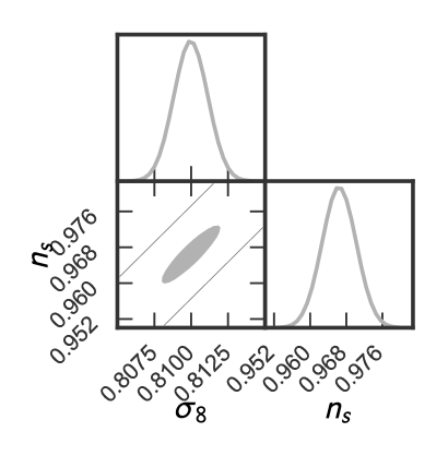
Figure 18: For Parametrization III with the smooth-k filter, the result of MCMC using all UV LFs and the $n_{s}$ prior. The $\sigma_{8}$ distribution is calculated from all samples.

Appendix B Full Results

We show the full results of the MCMC analysis using all UV LFs and $n_{s}$ prior. Fig. 19, 20, 21, 22, and 23 represent the results of Parametrization I, II, III, IV, and V, respectively. Fig.  24 is the result for Parametrization III but comparing the results with different filters.

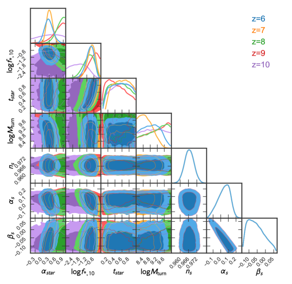
Figure 19: Result of MCMC using 24 parameters including astrophysical parameters in individual redshift bins (4 parameters $\times$ 5 redshift bins = 20 parameters), spectral index $n_{s}$ and PPS parameters. This result is for Parametrization I and discussed in Sec. III.1. For the constraints, we use UV LFs at all redshifts and Planck constraint on $n_{s}$ simultaneously.

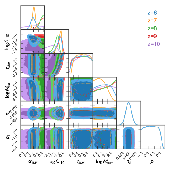
Figure 20: Same as Fig. 19, but for Parametrization II. This result is discussed in Sec. III.2.

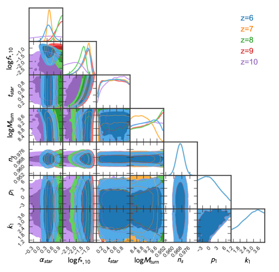
Figure 22: Same as Fig. 19, but for Parametrization IV. This result is discussed in Sec. III.4. This result is discussed in Sec. III.4.

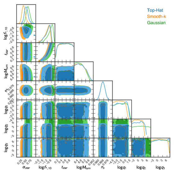
Figure 24: Result of MCMC using all LFs and Planck prior for various filters. The astrophysical parameter at $z=7$ is shown for reference. This result is discussed in Sec. III.3.

References

- Akrami et al. (2018) Y. Akrami et al. (Planck), Planck 2018 results. X. Constraints on inflation, arXiv:1807.06211 [astro-ph.CO] (2018).
- Bugaev and Klimai (2009) E. Bugaev and P. Klimai, Constraints on amplitudes of curvature perturbations from primordial black holes, Phys. Rev. D79, 103511 (2009), arXiv:0812.4247 [astro-ph] .
- Josan et al. (2009) A. S. Josan, A. M. Green, and K. A. Malik, Generalised constraints on the curvature perturbation from primordial black holes, Phys. Rev. D79, 103520 (2009), arXiv:0903.3184 [astro-ph.CO] .
- Sato-Polito et al. (2019) G. Sato-Polito, E. D. Kovetz, and M. Kamionkowski, Constraints on the primordial curvature power spectrum from primordial black holes, arXiv:1904.10971 [astro-ph.CO] (2019).
- Bringmann et al. (2012) T. Bringmann, P. Scott, and Y. Akrami, Improved constraints on the primordial power spectrum at small scales from ultracompact minihalos, Phys. Rev. D85, 125027 (2012), arXiv:1110.2484 [astro-ph.CO] .
- Emami and Smoot (2018) R. Emami and G. Smoot, Observational Constraints on the Primordial Curvature Power Spectrum, JCAP 1801 (01), 007, arXiv:1705.09924 [astro-ph.CO] .
- Kohri et al. (2013) K. Kohri, Y. Oyama, T. Sekiguchi, and T. Takahashi, Precise Measurements of Primordial Power Spectrum with 21 cm Fluctuations, JCAP 1310, 065, arXiv:1303.1688 [astro-ph.CO] .
- Sekiguchi et al. (2018) T. Sekiguchi, T. Takahashi, H. Tashiro, and S. Yokoyama, 21 cm Angular Power Spectrum from Minihalos as a Probe of Primordial Spectral Runnings, JCAP 1802 (02), 053, arXiv:1705.00405 [astro-ph.CO] .
- Muñoz et al. (2017) J. B. Muñoz, E. D. Kovetz, A. Raccanelli, M. Kamionkowski, and J. Silk, Towards a measurement of the spectral runnings, JCAP 1705, 032, arXiv:1611.05883 [astro-ph.CO] .
- Yoshiura et al. (2018) S. Yoshiura, K. Takahashi, and T. Takahashi, Impact of EDGES 21-cm global signal on the primordial power spectrum, Phys. Rev. D98, 063529 (2018), arXiv:1805.11806 [astro-ph.CO] .
- Yoshiura et al. (2020) S. Yoshiura, K. Takahashi, and T. Takahashi, Probing small scale primordial power spectrum with 21cm line global signal, Phys. Rev. D 101, 083520 (2020), arXiv:1911.07442 [astro-ph.CO] .
- Chluba et al. (2012) J. Chluba, A. L. Erickcek, and I. Ben-Dayan, Probing the inflaton: Small-scale power spectrum constraints from measurements of the CMB energy spectrum, Astrophys. J. 758, 76 (2012), arXiv:1203.2681 [astro-ph.CO] .
- Bouwens et al. (2017) R. J. Bouwens, P. A. Oesch, G. D. Illingworth, R. S. Ellis, and M. Stefanon, The z 6 Luminosity Function Fainter than -15 mag from the Hubble Frontier Fields: The Impact of Magnification Uncertainties, ApJ 843, 129 (2017), arXiv:1610.00283 [astro-ph.GA] .
- Oesch et al. (2018) P. A. Oesch, R. J. Bouwens, G. D. Illingworth, I. Labbé, and M. Stefanon, The Dearth of z 10 Galaxies in All HST Legacy Fields—The Rapid Evolution of the Galaxy Population in the First 500 Myr, ApJ 855, 105 (2018), arXiv:1710.11131 [astro-ph.GA] .
- Ishigaki et al. (2018) M. Ishigaki, R. Kawamata, M. Ouchi, M. Oguri, K. Shimasaku, and Y. Ono, Full-data Results of Hubble Frontier Fields: UV Luminosity Functions at z 6-10 and a Consistent Picture of Cosmic Reionization, ApJ 854, 73 (2018), arXiv:1702.04867 [astro-ph.GA] .
- Murray et al. (2013) S. G. Murray, C. Power, and A. S. G. Robotham, HMFcalc: An online tool for calculating dark matter halo mass functions, Astronomy and Computing 3, 23 (2013), arXiv:1306.6721 [astro-ph.CO] .
- Sheth et al. (2001) R. K. Sheth, H. J. Mo, and G. Tormen, Ellipsoidal collapse and an improved model for the number and spatial distribution of dark matter haloes, MNRAS 323, 1 (2001), arXiv:astro-ph/9907024 [astro-ph] .
- Lewis et al. (2000) A. Lewis, A. Challinor, and A. Lasenby, Efficient computation of CMB anisotropies in closed FRW models, ApJ 538, 473 (2000), arXiv:astro-ph/9911177 [astro-ph] .
- Eisenstein and Hu (1999) D. J. Eisenstein and W. Hu, Power Spectra for Cold Dark Matter and Its Variants, ApJ 511, 5 (1999), arXiv:astro-ph/9710252 [astro-ph] .
- Note (1) Https://camb.readthedocs.io.
- Leo et al. (2018) M. Leo, C. M. Baugh, B. Li, and S. Pascoli, A new smooth- space filter approach to calculate halo abundances, JCAP 1804, 010, arXiv:1801.02547 [astro-ph.CO] .
- Schneider (2015) A. Schneider, Structure formation with suppressed small-scale perturbations, MNRAS 451, 3117 (2015), arXiv:1412.2133 [astro-ph.CO] .
- Park et al. (2019) J. Park, A. Mesinger, B. Greig, and N. Gillet, Inferring the astrophysics of reionization and cosmic dawn from galaxy luminosity functions and the 21-cm signal, MNRAS 484, 933 (2019), arXiv:1809.08995 [astro-ph.GA] .
- Sun and Furlanetto (2016) G. Sun and S. R. Furlanetto, Constraints on the star formation efficiency of galaxies during the epoch of reionization, MNRAS 460, 417 (2016), arXiv:1512.06219 [astro-ph.GA] .
- Oke and Gunn (1983) J. B. Oke and J. E. Gunn, Secondary standard stars for absolute spectrophotometry., ApJ 266, 713 (1983).
- Harikane et al. (2016) Y. Harikane, M. Ouchi, Y. Ono, S. More, S. Saito, Y.-T. Lin, J. Coupon, K. Shimasaku, T. Shibuya, P. A. Price, L. Lin, B.-C. Hsieh, M. Ishigaki, Y. Komiyama, J. Silverman, T. Takata, H. Tamazawa, and J. Toshikawa, Evolution of Stellar-to-Halo Mass Ratio at z = 0 - 7 Identified by Clustering Analysis with the Hubble Legacy Imaging and Early Subaru/Hyper Suprime-Cam Survey Data, ApJ 821, 123 (2016), arXiv:1511.07873 [astro-ph.GA] .
- Foreman-Mackey et al. (2013) D. Foreman-Mackey, D. W. Hogg, D. Lang, and J. Goodman, emcee: The MCMC Hammer, PASP 125, 306 (2013), arXiv:1202.3665 [astro-ph.IM] .
- Goodman and Weare (2010) J. Goodman and J. Weare, Ensemble samplers with affine invariance, Communications in Applied Mathematics and Computational Science 5, 65 (2010).
- Shimizu et al. (2014) I. Shimizu, A. K. Inoue, T. Okamoto, and N. Yoshida, Physical properties of UDF12 galaxies in cosmological simulations, MNRAS 440, 731 (2014), arXiv:1310.0114 [astro-ph.CO] .
- Clay et al. (2015) S. J. Clay, P. A. Thomas, S. M. Wilkins, and B. M. B. Henriques, Galaxy formation in the Planck cosmology - III. The high-redshift universe, MNRAS 451, 2692 (2015), arXiv:1504.03321 [astro-ph.GA] .
- Ceverino et al. (2017) D. Ceverino, S. C. O. Glover, and R. S. Klessen, Introducing the FirstLight project: UV luminosity function and scaling relations of primeval galaxies, MNRAS 470, 2791 (2017), arXiv:1703.02913 [astro-ph.GA] .
- Rosdahl et al. (2018) J. Rosdahl, H. Katz, J. Blaizot, T. Kimm, L. Michel-Dansac, T. Garel, M. Haehnelt, P. Ocvirk, and R. Teyssier, The SPHINX cosmological simulations of the first billion years: the impact of binary stars on reionization, MNRAS 479, 994 (2018), arXiv:1801.07259 [astro-ph.GA] .
- Ma et al. (2018) X. Ma, P. F. Hopkins, S. Garrison-Kimmel, C.-A. Faucher-Giguère, E. Quataert, M. Boylan-Kolchin, C. C. Hayward, R. Feldmann, and D. Kereš, Simulating galaxies in the reionization era with FIRE-2: galaxy scaling relations, stellar mass functions, and luminosity functions, MNRAS 478, 1694 (2018), arXiv:1706.06605 [astro-ph.GA] .
- Tacchella et al. (2018) S. Tacchella, S. Bose, C. Conroy, D. J. Eisenstein, and B. D. Johnson, A Redshift-independent Efficiency Model: Star Formation and Stellar Masses in Dark Matter Halos at z 4, ApJ 868, 92 (2018), arXiv:1806.03299 [astro-ph.GA] .
- Hasegawa and Semelin (2013) K. Hasegawa and B. Semelin, The impacts of ultraviolet radiation feedback on galaxies during the epoch of reionization, MNRAS 428, 154 (2013), arXiv:1209.4143 [astro-ph.CO] .
- Santini et al. (2017) P. Santini, A. Fontana, M. Castellano, M. Di Criscienzo, E. Merlin, R. Amorin, F. Cullen, E. Daddi, M. Dickinson, J. S. Dunlop, A. Grazian, A. Lamastra, R. J. McLure, M. J. Michałowski, L. Pentericci, and X. Shu, The Star Formation Main Sequence in the Hubble Space Telescope Frontier Fields, ApJ 847, 76 (2017), arXiv:1706.07059 [astro-ph.GA] .
- Bhatawdekar and Conselice (2020) R. Bhatawdekar and C. J. Conselice, UV Spectral-Slopes at in the Hubble Frontier Fields: Lack of Evidence for Unusual or Pop III Stellar Populations, arXiv e-prints , arXiv:2006.00013 (2020), arXiv:2006.00013 [astro-ph.GA] .
- Bird et al. (2011) S. Bird, H. V. Peiris, M. Viel, and L. Verde, Minimally parametric power spectrum reconstruction from the Lyman forest, MNRAS 413, 1717 (2011), arXiv:1010.1519 [astro-ph.CO] .
- Chluba et al. (2019) J. Chluba et al., Spectral Distortions of the CMB as a Probe of Inflation, Recombination, Structure Formation and Particle Physics: Astro2020 Science White Paper, Bull. Am. Astron. Soc. 51, 184 (2019), arXiv:1903.04218 [astro-ph.CO] .
- Bocquet and Carter (2016) S. Bocquet and F. W. Carter, pygtc: beautiful parameter covariance plots (aka. giant triangle confusograms), The Journal of Open Source Software 1, 10.21105/joss.00046 (2016).
- Gillet et al. (2020) N. J. F. Gillet, A. Mesinger, and J. Park, Combining high-z galaxy luminosity functions with Bayesian evidence, MNRAS 491, 1980 (2020), arXiv:1906.06296 [astro-ph.GA] .
- Behroozi and Silk (2015) P. S. Behroozi and J. Silk, A Simple Technique for Predicting High-redshift Galaxy Evolution, ApJ 799, 32 (2015), arXiv:1404.5299 [astro-ph.GA] .