Kinetic theory of one-dimensional homogeneous long-range interacting systems
with an arbitrary potential of interaction

Abstract

Finite-$N$ effects unavoidably drive the long-term evolution of long-range interacting $N$-body systems. The Balescu-Lenard kinetic equation generically describes this process sourced by ${1/N}$ effects but this kinetic operator exactly vanishes by symmetry for one-dimensional homogeneous systems: such systems undergo a kinetic blocking and cannot relax as a whole at this order in ${1/N}$. It is therefore only through the much weaker ${1/N^{2}}$ effects, sourced by three-body correlations, that these systems can relax, leading to a much slower evolution. In the limit where collective effects can be neglected, but for an arbitrary pairwise interaction potential, we derive a closed and explicit kinetic equation describing this very long-term evolution. We show how this kinetic equation satisfies an $H$-theorem while conserving particle number and energy, ensuring the unavoidable relaxation of the system towards the Boltzmann equilibrium distribution. Provided that the interaction is long-range, we also show how this equation cannot suffer from further kinetic blocking, i.e., the ${1/N^{2}}$ dynamics is always effective. Finally, we illustrate how this equation quantitatively matches measurements from direct $N$-body simulations.

I Introduction

The statistical mechanics and kinetic theory of systems with long-range interactions is a topic of great interest Campa et al. (2014) because of its unusual properties (ensembles inequivalence, negative specific heats, non-Boltzmannian quasistationary states, instabilities, phase transitions…) and its applications in various domains of physics such as plasma physics Nicholson (1992), astrophysics Binney and Tremaine (2008), or two-dimensional hydrodynamics Chavanis (2002); Bouchet and Venaille (2012).

Closed systems with long-range interactions generically experience two successive types of relaxations. There is first a fast collisionless relaxation driven by the mean field towards a non-Boltzmannian quasistationary state. This corresponds to the process of violent relaxation described by Lynden-Bell Lynden-Bell (1967) for collisionless stellar systems governed by the Vlasov-Poisson equations (see, e.g., Chavanis et al. (1996)). This phase takes place within a few dynamical times (independent of the number of particles) and ends when the system has reached a virialized state, i.e., a stable steady state of the Vlasov equation. Then, a slow collisional relaxation towards the Boltzmann distribution of statistical equilibrium takes place. It is driven by discreteness effects (granularities) due to finite values of $N$, the total number of particles. The relaxation time expressed in units of the dynamical time diverges with the number of particles $N$. In this sense, the lifetime of the quasistationary state becomes infinite when $N\rightarrow+\infty$. Nevertheless, for large but finite values of $N$, the system evolves secularly, passing adiabatically by a succession of quasistationary states.

The derivation of kinetic equations describing the secular evolution of systems with long-range interactions has a rich history (see, e.g., the introduction of Chavanis (2013a, b) for a short account). Landau Landau (1936) first derived a kinetic equation for Coulombian neutral plasmas by expanding the Boltzmann Boltzmann (1872) equation in terms of a small deflection parameter, namely the velocity deviation experienced by a particle during a “collision”. An equivalent kinetic equation was obtained independently by Chandrasekhar Chandrasekhar (1943) (and generalized by Rosenbluth et al. Rosenbluth et al. (1957)) for stellar systems. Chandrasekhar started from the Fokker-Planck equation and calculated the diffusion and friction coefficients using an impulse approximation. However, the approaches of Landau and Chandrasekhar have a phenomenological character and ignore collective effects and spatial inhomogeneity. This leads to difficulties such as the logarithmic divergence of the collision term at large impact parameters.

Systematic and rigorous approaches directly starting from the $N$-body dynamics (or from the Liouville equation) were developed by Bogoliubov Bogoliubov (1946) using a hierarchy of equations for the reduced distribution functions (nowadays called the BBGKY hierarchy) and by Prigogine and Balescu Prigogine and Balescu (1959) using diagrammatic techniques. These hierarchies of equations may be closed by considering an expansion of the equations in powers of the small coupling parameter $1/N$ (with ${N\gg 1}$) which measures the strength of the correlation functions. Initially, only two-body correlation functions, which are of order $1/N$, were taken into account. This corresponds to the weak coupling approximation of plasma physics. These methods led to the Balescu-Lenard equation Balescu (1960); Lenard (1960) which takes into account collective effects (dynamical Debye shielding) thereby removing the logarithmic divergence that occurs in the Landau equation at large scales. This kinetic equation describes the effect of two-body encounters and is essentially exact at order $1/N$. It can also be derived from a quasilinear theory based on the Klimontovich equation for the discrete distribution function Klimontovich (1967). The original Balescu-Lenard equation (applying to neutral plasmas) is valid for spatially homogeneous systems but it has recently been generalized to inhomogeneous systems by using angle-action variables Heyvaerts (2010); Chavanis (2012a) with specific applications to self-gravitating systems Fouvry et al. (2015, 2017); Hamilton et al. (2018); Bar-Or and Fouvry (2018) and to the magnetized phase of the Hamiltonian Mean Field (HMF) model Benetti and Marcos (2017). More generally, the Balescu-Lenard kinetic equation is valid for any system with long-range interactions in arbitrary dimension of space Chavanis (2012b). For usual three-dimensional (3D) systems, this kinetic equation conserves the particle number and the energy, and satisfies an $H$-theorem for the Boltzmann entropy. As a result, it relaxes towards the Boltzmann distribution which is the maximum entropy state (most probable state) at fixed particle number and energy. Since the Balescu-Lenard equation is valid at order $1/N$ it describes the relaxation of the system on a timescale of order $Nt_{\mathrm{d}}$, with $t_{\mathrm{d}}$ the dynamical time. Actually, for Coulombian plasmas and stellar systems, there is a logarithmic correction due to strong collisions at small impact parameters, so that the relaxation time scales as ${(N/\ln N)t_{\mathrm{d}}}$.

Apart from specificities inherent to systems with long-range interactions (the process of violent relaxation, the existence of transient non-Boltzmannian quasistationary states, the very long relaxation time, the need to account for spatially inhomogeneous distributions, and the importance of collective effects) the results of the kinetic theory at order $1/N$ are consistent with the original Boltzmann picture of relaxation in a dilute gas. In a sense, the Balescu-Lenard equation (and more specifically the homogeneous Landau equation) is a descendent of the Boltzmann equation: the collision term is the product of two distribution functions ${F(1)F(2)}$ characteristic of any two-body collision term and the derivation of the conservation laws and of the $H$-theorem is essentially the same as that given by Boltzmann.

However, for 1D homogeneous systems, the Balescu-Lenard collision term vanishes identically. As a result, the dynamics sourced by two-body correlations is frozen at order ${1/N}$, so that there is no evolution of the overall distribution on a timescale ${Nt_{\mathrm{d}}}$. This is a situation of kinetic blocking. The system is therefore expected to evolve dynamically under the effect of nontrivial three-body (or higher) correlations implying that the relaxation time should scale as ${N^{2}t_{\mathrm{d}}}$ (or be even larger). The peculiarity of 1D homogeneous systems was first noticed by Eldrige and Feix Eldridge and Feix (1963) in the context of 1D plasmas Dawson (1962). They showed that the Balescu-Lenard collision term vanishes and conjectured the existence of a non-zero ${1/N^{2}}$ collision term. The corresponding ${N^{2}t_{\mathrm{d}}}$ scaling of the relaxation time was confirmed by Dawson Dawson (1964) from direct $N$-body simulations. Later, Rouet and Feix Rouet and Feix (1991) illustrated the striking difference that exists between the relaxation of the system as a whole (overall distribution) which takes place on a timescale ${N^{2}t_{\mathrm{d}}}$ and the relaxation of test (or labelled) particles which takes place on a timescale ${Nt_{\mathrm{d}}}$. The stochastic evolution of the test particles is governed by a Fokker-Planck equation which can be obtained from the Balescu-Lenard equation by making a bath approximation, i.e., by fixing the distribution of the field particles. This procedure transforms an integro-differential equation into a differential equation. Since in 1D the test particles acquire the distribution of the field particles (bath) whatever its distribution function (while this is true only for the Boltzmann distribution in 3D) this explains why a 1D homogeneous system does not evolve on a timescale ${Nt_{\mathrm{d}}}$.

Similar results were found later for axisymmetric distributions of 2D point vortices when the profile of angular velocity ${\Omega(r,t)}$ is monotonic Dubin and O’Neil (1988); Chavanis (2001); Dubin (2003); Chavanis and Lemou (2007); Chavanis (2012c, d) and for 1D systems with long-range interactions such as the HMF model Bouchet and Dauxois (2005); Chavanis et al. (2005) and classical spin systems with anisotropic interaction (or equivalently long-range interacting particles moving on a sphere) Gupta and Mukamel (2011); Barré and Gupta (2014); Lourenço and Rocha Filho (2015); Fouvry et al. (2019a). In the context of the HMF model, it was first believed that the relaxation time was anomalous, scaling with the number of particles as ${N^{1.7}t_{\mathrm{d}}}$ Yamaguchi et al. (2004). However, it was later demonstrated Rocha Filho et al. (2014a, b); Fouvry et al. (2019b) that this anomalous exponent was due to small size effects and that the correct scaling is indeed ${N^{2}t_{\mathrm{d}}}$ in agreement with kinetic theory Chavanis (2012b). The collisional relaxation of the HMF model was studied by Campa et al. (2008) who found that, for certain initial conditions, the distribution function ${F(v,t)}$ can be fitted by polytropes with a time-dependent index. When the polytropic index reaches a critical value, the distribution function becomes dynamically unstable (with respect to the Vlasov equation) and a dynamical phase transition from a homogeneous phase to an inhomogeneous phase takes place. These authors stressed the importance of deriving an explicit kinetic equation at order ${1/N^{2}}$ in order to study the collisional relaxation of 1D homogeneous systems in greater detail.

A first step in that direction was made by Rocha Filho et al. (2014b). They started from the equations of the BBGKY hierarchy truncated at order ${1/N^{2}}$, neglected collective effects, and used a computer algebra system to solve the truncated hierarchy of equations. However, the form of the collision term that they obtained was not suitable to study the kinetic equation in detail and solve it. A second step was made by Fouvry et al. (2019b) who used a similar procedure and obtained a more tractable expression of the kinetic equation at order $1/N^{2}$. They proved its well-posedness and established its main properties: conservation laws, $H$-theorem, and relaxation towards the Boltzmann distribution. They also carried out detailed comparisons with direct numerical simulations and found a good agreement at sufficiently high temperatures where collective effects (that are neglected in their kinetic equation) are weak enough. The kinetic equation at order $1/N^{2}$ is fundamentally different from the Boltzmann equation (or from the related Landau and Balescu-Lenard equations) because it involves the product of three distribution functions instead of just two, in line with the fact that the evolution is driven by three-body correlations instead of two-body correlations. Therefore, it is remarkable that an $H$-theorem can still be proven in this case by a method which is completely different from that of Boltzmann. This highlights that the validity of the $H$-theorem goes beyond the original Boltzmann picture. This also gives a more general justification (from the kinetic theory angle) of the maximum entropy principle that is used to determine the statistical equilibrium state of the system.

The kinetic equation derived in Fouvry et al. (2019b) was restricted to the HMF model, i.e., to a potential of interaction which involves only one Fourier mode. In the present paper, we go beyond these limitations, namely, we generalize the kinetic equation to an arbitrary potential of interaction. This is an important generalization because it allows us to treat more general situations of physical interest spanning a wider variety of long-range interacting potentials. In the limit where collective effects can be neglected, i.e., in the limit of dynamically hot systems that only weakly amplify perturbations, we present a closed and explicit kinetic equation generically describing the collisional relaxation of the system on ${N^{2}t_{\mathrm{d}}}$ timescales, as driven by three-body correlations. Strikingly, for long-range interactions, we show that no further kinetic blocking is possible. Finally, in addition to exploring the generic properties of this collision operator, we also quantitatively compare its predictions with direct $N$-body simulations.

The paper is organised as follows. In Section II, we present the kinetic equation describing relaxation at order ${1/N^{2}}$, as given by Eq. (4). The detailed procedure used to derive that equation is described in Appendix A, while the effective calculations were performed using a computer algebra system (see Supplemental Material (Fouvry et al., 2020)). In Section III, we present the main properties of this kinetic equation, in particular its conservation laws and its $H$-theorem. In Section IV, we explore in detail the steady states of this kinetic equation, highlighting in particular that, as long as the interaction potential is long-range, ${1/N^{2}}$ effects unavoidably lead to the full relaxation of the system towards the Boltzmann distribution. In Section V, we show that the kinetic equation is well-posed, i.e., that one can compute explicitly its prediction. In Section VI, we illustrate how this equation quantitatively matches measurements from direct numerical simulations, for initial conditions dynamically hot enough. Finally, we conclude in Section VII.

II The kinetic equation

We are interested in the long-term dynamics of a (periodic) 1D long-range interacting system. We assume that it is composed of $N$ particles of individual mass ${\mu=M_{\mathrm{tot}}/N}$, with $M_{\mathrm{tot}}$ the system’s total mass. The canonical phase space coordinates are denoted by ${(\theta,v)}$, with $\theta$ a ${2\pi}$-periodic angle and $v$ the velocity. The system’s total Hamiltonian then reads

$$H=\frac{1}{2}\sum_{i=1}^{N}v_{i}^{2}+\mu\sum_{i<j}^{N}U(\theta_{i},\theta_{j}),$$ (1)

where ${U(\theta_{i},\theta_{j})}$ stands for the considered pairwise interaction potential. We naturally assume that the potential satisfies the symmetries ${U(\theta_{i},\theta_{j})=U(|\theta_{i}-\theta_{j}|)}$. As such, it can be expanded in Fourier-space as

$$U(\theta_{1},\theta_{2})=-\sum_{k}U_{k}\,\mathrm{e}^{\mathrm{i}k(\theta_{1}-\theta_{2})},$$ (2)

where the coefficients, ${U_{k}\in\mathbb{R}}$, satisfy the symmetry ${U_{-k}=U_{k}}$. In Eq. (2), we also introduced an overall negative sign, so that one generically has ${U_{k}\geq 0}$ for an attractive potential.

For an homogeneous system, the instantaneous state of the system is described by its velocity distribution function (DF), ${F(v,t)}$, which we normalise as ${\!\int\!\mathrm{d}\theta\mathrm{d}vF=M_{\mathrm{tot}}}$, with $M_{\mathrm{tot}}$ the total mass of the system. To describe the long-term relaxation of the system, one must characterise the long-term evolution of that DF through a closed self-consistent kinetic equation.

As derived in Heyvaerts (2010); Chavanis (2012a) and references therein, if one limits oneself only to ${1/N}$ effects, the dynamics of ${F(v,t)}$ is described by the homogeneous Balescu-Lenard equation. With the present notation, it reads

$$\frac{\partial F(v)}{\partial t}= \,2\pi^{2}\mu\frac{\partial}{\partial v}\bigg{[}\sum_{k}\frac{|k|\,|U_{k}|^{2}}{|\varepsilon_{k}(k\,v)|^{2}}$$

$$\times \,\!\!\int\!\!\mathrm{d}v_{1}\,\delta_{\mathrm{D}}(v\!-\!v_{1})\,\bigg{(}\frac{\partial}{\partial v}\!-\!\frac{\partial}{\partial v_{1}}\bigg{)}F(v)F(v_{1})\bigg{]},$$ (3)

where the time dependence of the DFs was dropped to shorten the notations. In that equation, we also introduced the dielectric function, ${\varepsilon_{k}(\omega)}$, whose explicit expression is given in Eq. (64).

Because of the resonance condition, ${\delta_{\mathrm{D}}(v-v_{1})}$, the diffusion flux from the Balescu-Lenard equation (3) exactly vanishes. Indeed, only local two-body resonances of the form ${v=v_{1}}$ are permitted, which, because of the exact local cancellation of the sum of the drift and diffusion coefficients, cannot drive any relaxation of the system’s mean DF. One-dimensional homogeneous systems are generically kinetically blocked w.r.t. two-body correlations at order ${1/N}$. This drastically slows down the system’s long-term evolution. As a consequence, it is only through weaker three-body correlations, via ${1/N^{2}}$ effects, that such systems can relax to their thermodynamical equilibrium. This is the dynamics on which the present paper is focused.

On the one hand, the effective derivation of the system’s appropriate kinetic equation is straightforward, as the roadmap to follow is systematic. On the other hand, these calculations rapidly become cumbersome in practice given the large numbers of terms that one has to deal with. In addition, to finally reach a simple closed form, one also has to perform numerous symmetrisations and relabellings. All in all, to alleviate the technical aspects of these calculations, we carried out all our derivation using Mathematica with a code that can be found in the Supplemental Material (Fouvry et al., 2020). In this paper, we will restrict ourselves to the outline of the derivation.

The key details of our approach are spelled out in Appendix A. In a nutshell, the main steps of the derivation are as follows. (i) First, we derive the usual coupled BBGKY evolution equations for the one-, two-, and three-body distribution functions, i.e., the equations that fully encompass the system’s dynamics at order ${1/N^{2}}$. (ii) Using the cluster expansion (Balescu, 1997), we can rewrite these evolution equations as coupled equations for the one-body DF, ${F(v,t)}$, and the two- and three-body correlation functions. At this stage, the evolution equations are still coupled to each other, but are ordered w.r.t. the small parameter ${1/N}$. (iii) We may then truncate these equations at order ${1/N^{2}}$. In addition, at this stage, we also neglect the contribution from collective effects, assuming that the system is dynamically hot so that it is not efficient at self-consistently amplifying perturbations. Another key trick is to split the two-body correlation functions in two components, respectively associated with the ${1/N}$ and ${1/N^{2}}$ contributions. (iv) Finally, having set up a set of four (well-posed) coupled partial differential equations, we may solve them explicitly in time. At that stage, the key assumption is Bogoliubov’s ansatz, i.e., the assumption that the system’s mean DF evolves on timescales much longer than its correlation functions. Following various relabellings, symmetrisations, and integrations by part, we finally obtain an explicit and closed expression for the system’s ${1/N^{2}}$ collision operator. The hardest part of this calculation is the appropriate use of the resonance conditions to simplify accordingly the arguments of the functions appearing in the kinetic equation.

All in all, the kinetic equation then reads

$$\frac{\partial F(v)}{\partial t}=2\pi^{3}\mu^{2} \,\frac{\partial}{\partial v}\bigg{[}\!\sum_{k_{1},k_{2}}\!\!\frac{k_{2}^{2}}{k_{1}^{2}(k_{1}\!+\!k_{2})}\,\mathcal{U}(k_{1},k_{2})\,\mathcal{P}\!\!\int\!\!\frac{\mathrm{d}v_{1}}{(v\!-\!v_{1})^{4}}$$

$$\,\times\!\!\int\!\!\mathrm{d}v_{2}\,\delta_{\mathrm{D}}\big{[}\mathbf{k}\cdot\mathbf{v}\big{]}\bigg{(}\mathbf{k}\cdot\frac{\partial}{\partial\mathbf{v}}\bigg{)}F_{3}(\mathbf{v})\bigg{]},$$ (4)

where the sum over ${k_{1},k_{2}}$ is restricted to the indices such that $k_{1}$, $k_{2}$, and ${(k_{1}\!+\!k_{2})}$ are all non-zero. In Eq. (4), to shorten the notations, we introduced the velocity vector ${\mathbf{v}=(v,v_{1},v_{2})}$, as well as ${F_{3}(\mathbf{v})=F(v)F(v_{1})F(v_{2})}$. Finally, we introduced the resonance vector

$$\mathbf{k}=\big{(}k_{1}\!+\!k_{2},-k_{1},-k_{2}\big{)}$$ (5)

as well as the coupling factor

$$\mathcal{U}(k_{1},k_{2})\!=\!\big{(}(k_{1}\!+\!k_{2})U_{k_{1}}U_{k_{2}}\!-\!k_{1}U_{k_{1}+k_{2}}U_{k_{2}}\!-\!k_{2}U_{k_{1}+k_{2}}U_{k_{1}}\big{)}^{2}.$$ (6)

In Eq. (4), we also introduced Cauchy’s principal value, as $\mathcal{P}$, which acts on the integral ${\!\int\!\mathrm{d}v_{1}}$. We postpone to Section V the proof of its well-posedness.

Of course, the similarities between the ${1/N}$ Balescu-Lenard equation (3) and the present ${1/N^{2}}$ equation are striking. We emphasise that Eq. (4) is proportional to ${\mu^{2}\sim 1/N^{2}}$, so that it effectively describes a (very) slow relaxation on ${N^{2}t_{\mathrm{d}}}$ timescales. In addition, we also note that the collision operator involves the DF three times, which stems from the fact that the relaxation is sourced by three-body correlations. Such correlations are coupled through a resonance condition on three distinct velocities, namely via the factor ${\delta_{\mathrm{D}}[\mathbf{k}\cdot\mathbf{v}]}$. This is one of the key changes w.r.t. to the ${1/N}$ kinetic equation (3), as the present three-body resonances allow for non-trivial and non-local kinetic couplings, driving a non-vanishing overall relaxation. Equation (4) also differs from Eq. (3) in one other significant manner, in as much as it does not involve the dielectric function, ${\varepsilon_{k}(\omega)}$, since collective effects have been neglected at this stage (we suggest in footnote 7 how collective effects may be accounted for in Eq. (4)).

Equation (4) is the main result of the paper: this closed and explicit kinetic equation is the appropriate self-consistent kinetic equation to describe the long-term evolution of a dynamically hot one-dimensional homogeneous system, as driven by ${1/N^{2}}$ effects. It is quite general since Eq. (4) applies to any arbitrary long-range interaction potentials, as defined in Eq. (2). Finally, Eq. (4) holds as long as the system remains linearly Vlasov stable, to prevent it from being driven to an inhomogeneous state.

III Properties

In this section, we explore some of the key properties of the kinetic equation (4).

III.1 Conservation laws

The kinetic equation (4) satisfies various conservation laws, in particular the conservation of the total mass, ${M(t)}$, momentum, ${P(t)}$, and energy, ${E(t)}$. Ignoring irrelevant prefactors, these quantities are defined as

$$M(t) \,=\!\!\int\!\!\mathrm{d}v\,F(v,t),$$

$$P(t) \,=\!\!\int\!\!\mathrm{d}v\,v\,F(v,t),$$

$$E(t) \,=\!\!\int\!\!\mathrm{d}v\,\tfrac{1}{2}v^{2}\,F(v,t).$$ (7)

To recover the conservation of these quantities, let us first rewrite Eq. (4) as

$$\frac{\partial F(v)}{\partial t}=\frac{\partial}{\partial v}\,\mathcal{F}(v,t),$$ (8)

with ${\mathcal{F}(v,t)}$ the diffusion flux. We can then rewrite the time derivatives of Eq. (7) as

$$\frac{\mathrm{d}M}{\mathrm{d}t} \,=\!\!\int\!\!\mathrm{d}v\,\frac{\partial}{\partial v}\,\mathcal{F}(v,t),$$

$$\frac{\mathrm{d}P}{\mathrm{d}t} \,=-\!\!\int\!\!\mathrm{d}v\,\mathcal{F}(v,t),$$

$$\frac{\mathrm{d}E}{\mathrm{d}t} \,=-\!\!\int\!\!\mathrm{d}v\,v\,\mathcal{F}(v,t).$$ (9)

The conservation of the total mass then follows from the absence of any boundary contributions, so that one has ${\mathrm{d}M/\mathrm{d}t=0}$.

Recovering the conservation of ${P(t)}$ and ${E(t)}$ requires a bit more finesse, as one needs to leverage the symmetry properties of the terms involved. The main trick is to study the symmetries of the term ${\!\int\!\mathrm{d}v\,\mathcal{F}(v)}$. One can write

$$\!\!\int\!\!\mathrm{d}v\,\mathcal{F}(v)=\sum_{k_{1},k_{2}}(k_{1}\!+\!k_{2})\!\!\int\!\!\mathrm{d}v\mathrm{d}v_{1}\mathrm{d}v_{2}\,A_{k_{1}k_{2}}(v,v_{1},v_{2}),$$ (10)

where the expression of ${A_{k_{1}k_{2}}(v,v_{1},v_{2})}$ follows from Eq. (10) and reads

$$A_{k_{1}k_{2}}(v,v_{1},v_{2})= \,2\pi^{3}\mu^{2}\frac{k_{2}^{2}}{k_{1}^{2}(k_{1}\!+\!k_{2})^{2}}\mathcal{U}(k_{1},k_{2})\,\mathcal{P}\!\!\int\!\!\frac{\mathrm{d}v_{1}}{(v-v_{1})^{4}}$$

$$\,\times\!\!\int\!\!\mathrm{d}v_{2}\,\delta_{\mathrm{D}}\big{[}\mathbf{k}\cdot\mathbf{v}\big{]}\,\bigg{(}\!\mathbf{k}\cdot\frac{\partial}{\partial\mathbf{v}}\!\bigg{)}\,F_{3}(\mathbf{v}).$$ (11)

Starting from Eq. (10), one can first perform the relabellings ${\{v,v_{1}\}\to\{v_{1},v_{2}\}}$ and ${\{k_{1},k_{2}\}\to\{-k_{1}-k_{2},k_{2}\}}$. Following these changes, which are more easily performed using a computer algebra system (Fouvry et al., 2020), Eq. (10) becomes

$$\!\!\int\!\!\mathrm{d}v\,\mathcal{F}(v)=-\sum_{k_{1},k_{2}}k_{1}\!\!\int\!\!\mathrm{d}v\mathrm{d}v_{1}\mathrm{d}v_{2}\,A_{k_{1}k_{2}}(v,v_{1},v_{2}).$$ (12)

Similarly, starting once again from Eq. (10), one can also perform the relabellings ${\{v,v_{2}\}\to\{v_{2},v_{1}\}}$ and ${\{k_{1},k_{2}\}\to\{-k_{1},k_{1}+k_{2}\}}$. Following these changes, Eq. (10) becomes

$$\!\!\int\!\!\mathrm{d}v\,\mathcal{F}(v)=-\sum_{k_{1},k_{2}}k_{2}\!\!\int\!\!\mathrm{d}v\mathrm{d}v_{1}\mathrm{d}v_{2}\,A_{k_{1}k_{2}}(v,v_{1},v_{2}).$$ (13)

Having obtained the symmetrised expressions from Eqs. (10), (12), and (13), we can now go back to the computation of the conserved quantities from Eq. (9). By adding ${\tfrac{1}{3}}$ of every expression, we obtain

$$\frac{\mathrm{d}P}{\mathrm{d}t} \,=-\frac{1}{3}\sum_{k_{1},k_{2}}\!\!\int\!\!\mathrm{d}v\mathrm{d}v_{1}\mathrm{d}v_{2}\,A_{k_{1}k_{2}}(v,v_{1},v_{2})$$

$$\;\;\;\;\;\;\;\;\;\;\;\times\bigg{\{}(k_{1}\!+\!k_{2})-k_{1}-k_{2}\bigg{\}}$$

$$\,=0.$$ (14)

We can proceed very similarly for the total energy, repeating the symmetrisations which were performed to obtain the various rewritings of the integral of the flux. Equation (9) becomes

$$\frac{\mathrm{d}E}{\mathrm{d}t} \,=-\frac{1}{3}\sum_{k_{1},k_{2}}\!\!\int\!\!\mathrm{d}v\mathrm{d}v_{1}\mathrm{d}v_{2}\,A_{k_{1}k_{2}}(v,v_{1},v_{2})$$

$$\;\;\;\;\;\;\;\;\;\;\;\times\bigg{\{}(k_{1}\!+\!k_{2})v-k_{1}v_{1}-k_{2}v_{2}\bigg{\}}$$

$$\,=0,$$ (15)

owing to the presence of the resonance condition ${\delta_{\mathrm{D}}[(k_{1}\!+\!k_{2})v\!-\!k_{1}v_{1}\!-\!k_{2}v_{2}]}$ in the expression of ${A_{k_{1}k_{2}}(v,v_{1},v_{2})}$ in Eq. (11).

III.2 $H$-theorem

Let us define the system’s entropy as

$$S(t)=-\!\!\int\!\!\mathrm{d}v\,s\big{(}F(v,t)\big{)},$$ (16)

with ${s(F)=F\,\ln(F)}$ Boltzmann’s entropy. Following the definition from Eq. (8), the time derivative of Eq. (16) reads

$$\frac{\mathrm{d}S}{\mathrm{d}t}=\!\!\int\!\!\mathrm{d}v\,\frac{F^{\prime}(v)}{F(v)}\,\mathcal{F}(v,t).$$ (17)

To show that the system’s entropy unavoidably and systematically grows with time, we use the same approach as in the previous section. Repeating the symmetrisations which were performed in Eqs. (12) and (13), we can rewrite Eq. (17) as

$$\frac{\mathrm{d}S}{\mathrm{d}t}= \,\frac{1}{3}\sum_{k_{1},k_{2}}\!\!\int\!\!\mathrm{d}v\mathrm{d}v_{1}\mathrm{d}v_{2}\,A_{k_{1}k_{2}}(v,v_{1},v_{2})$$

$$\times \,\bigg{\{}(k_{1}\!+\!k_{2})\,\frac{F^{\prime}(v)}{F(v)}-k_{1}\frac{F^{\prime}(v_{1})}{F(v_{1})}-k_{2}\frac{F^{\prime}(v_{2})}{F(v_{2})}\bigg{\}}.$$ (18)

Luckily, returning to the definition of ${A_{k_{1}k_{2}}}$ from Eq. (11), we note that Eq. (18) can be rewritten under the form

$$\frac{\mathrm{d}S}{\mathrm{d}t} \,=\frac{2\pi^{3}\mu^{2}}{3}\sum_{k_{1},k_{2}}\!\!\int\!\!\mathrm{d}v\mathrm{d}v_{1}\mathrm{d}v_{2}\,\frac{k_{2}^{2}}{k_{1}^{2}(k_{1}\!+\!k_{2})^{2}}\,\mathcal{U}(k_{1},k_{2})$$

$$\,\times\mathcal{P}\bigg{(}\!\frac{1}{(v-v_{1})^{4}}\!\bigg{)}\,\frac{\delta_{\mathrm{D}}\big{[}\mathbf{k}\cdot\mathbf{v}\big{]}}{F_{3}(\mathbf{v})}$$

$$\,\times\bigg{(}(k_{1}\!+\!k_{2})\frac{F^{\prime}(v)}{F(v)}-k_{1}\frac{F^{\prime}(v_{1})}{F(v_{1})}-k_{2}\frac{F^{\prime}(v_{2})}{F(v_{2})}\bigg{)}^{2}.$$ (19)

As all the terms in these integrals are positive, in particular the interaction coupling ${\mathcal{U}(k_{1},k_{2})}$ from Eq. (6), the kinetic equation (4) therefore satisfies an $H$-theorem, i.e., one has

$$\frac{\mathrm{d}S}{\mathrm{d}t}\geq 0.$$ (20)

This is the essential result of the present section, as we have just proven that the kinetic equation (4) unavoidably leads to an irreversible relaxation of the system. In Section IV, we will use the expression of the entropy increase from Eq. (19) to determine which DFs are the equilibrium states of the diffusion, i.e., which DFs satisfy ${\mathrm{d}S/\mathrm{d}t=0}$.

III.3 Dimensionless rescaling

We introduce the system’s velocity dispersion as

$$\sigma^{2}=\frac{1}{M_{\mathrm{tot}}}\!\!\int\!\!\mathrm{d}\theta\mathrm{d}v\,v^{2}\,F(v).$$ (21)

This entices us then to also introduce the dimensionless velocity, $u$, and time, $\overline{t}$, as

$$u=\frac{v}{\sigma}\;\;\;;\;\;\;\overline{t}=\frac{t}{t_{\mathrm{d}}},$$ (22)

with ${t_{\mathrm{d}}=1/\sigma}$ the system’s dynamical time. Similarly, it is natural to introduce the dimensionless probability distribution function (PDF)

$$\overline{F}(u)=\frac{2\pi\sigma}{M_{\mathrm{tot}}}\,F(u\sigma),$$ (23)

which satisfies the normalisation condition ${\!\int\!\mathrm{d}u\overline{F}(u)=1}$. We note that this PDF has a (dimensionless) unit velocity dispersion given by ${\!\int\!\mathrm{d}u\,u^{2}\overline{F}(u)=1}$. Finally, we must also introduce a quantity to assess the dynamical temperature of the system, and the strength of the associated underlying collective effects. Following Appendix B, we define the dimensionless stability parameter

$$Q=\frac{\sigma^{2}}{U_{\mathrm{max}}M_{\mathrm{tot}}},$$ (24)

where we introduced ${U_{\mathrm{max}}=\max_{k}U_{k}}$. The larger $Q$, the hotter the system, i.e., the weaker the collective effects. Given $U_{\mathrm{max}}$, we may finally define the dimensionless interaction coefficients ${\overline{U}_{k}=U_{k}/U_{\mathrm{max}}}$.

Using these conventions, we can rewrite Eq. (4) under the dimensionless form

$$\,\frac{\partial\overline{F}(u)}{\partial\overline{t}}\!=\!\frac{\pi}{2}\frac{1}{Q^{4}N^{2}}\frac{\partial}{\partial u}\bigg{[}\sum_{k_{1},k_{2}}\!\!\frac{k_{2}^{2}}{k_{1}^{2}(k_{1}\!+\!k_{2})}\overline{\mathcal{U}}(k_{1},k_{2})\,$$

$$\times\mathcal{P}\!\!\int\!\!\frac{\mathrm{d}u_{1}}{(u\!-\!u_{1})^{4}}\!\!\int\!\!\mathrm{d}u_{2}\bigg{\{}\delta_{\mathrm{D}}\big{[}\mathbf{k}\cdot\mathbf{u}\big{]}\bigg{(}\!\mathbf{k}\cdot\frac{\partial}{\partial\mathbf{u}}\!\bigg{)}\,\overline{F}_{3}(\mathbf{u})\bigg{\}}\bigg{]},$$ (25)

where the coupling factor ${\overline{\mathcal{U}}(k_{1},k_{2})}$ naturally follows from Eq. (6) with the replacement ${U_{k}\to\overline{U}_{k}}$. Finally, Eq. (25) can be rewritten as a continuity equation, reading

$$\frac{\partial\overline{F}(u)}{\partial\overline{t}}=\frac{\pi}{2}\frac{1}{Q^{4}N^{2}}\,\frac{\partial}{\partial u}\big{[}\,\overline{\mathcal{F}}(u)\big{]},$$ (26)

where the dimensionless instantaneous flux, ${\overline{\mathcal{F}}(u)}$, follows from Eq. (25).

Equation (25) is an enlightening rewriting of the kinetic equation, as it clearly highlights the expected relaxation time of a given system. Assuming that the term within brackets is of order unity, Eq. (25) states therefore that the relaxation time, $t_{\mathrm{r}}$, of the system scales like

$$t_{\mathrm{r}}\simeq Q^{4}N^{2}t_{\mathrm{d}}.$$ (27)

In particular, we recover that the hotter the system, the slower the long-term relaxation. As Eq. (4) was derived while neglecting collective effects, i.e., in the limit ${Q\gg 1}$, the relaxation will only occur on very very long timescales because of the factor $Q^{4}$ in Eq. (27).

IV Steady states

In the previous section, we showed that Eq. (4) satisfies an H-theorem for the Boltzmann entropy. Let us now explore what are the steady states of that evolution equation, i.e., the DFs such that Eq. (4) predicts ${\partial F/\partial t=0}$.

IV.1 Boltzmann distribution

We expect the thermodynamical equilibria originating from relaxation to take the form of (possibly shifted) homogeneous Boltzmann DF reading

$$F_{\mathrm{B}}(v)=C\,\mathrm{e}^{-\beta(v-v_{0})^{2}},$$ (28)

with $\beta$ the inverse temperature, and $C$ a normalisation constant. These DFs maximise the Boltzmann entropy at fixed mass, momentum, and energy. It is straightforward to check that such DFs are equilibrium solutions of the kinetic equation (4). Indeed, noting that the vector $\mathbf{k}$ from Eq. (5) is of zero sum, we can write

$$\frac{\partial F_{\mathrm{B}}(v)}{\partial t}\propto\delta_{\mathrm{D}}\big{[}\mathbf{k}\cdot\mathbf{v}\big{]}\,\big{(}\mathbf{k}\cdot\mathbf{v}\big{)}=0.$$ (29)

This is an important result, as it highlights that homogeneous Boltzmann distributions are indeed equilibrium solutions of the ${1/N^{2}}$ kinetic equation (4). In the coming sections, thanks to the H-theorem, we will strengthen this result by showing that homogeneous Boltzmann DFs are in fact the only equilibrium solutions of the present kinetic equation, whatever the considered long-range interacting potential.

IV.2 Constraint from the H-theorem

Following the computation of ${\mathrm{d}S/\mathrm{d}t}$ in Eq. (20), we can now determine what are the most generic steady states of the kinetic equation (4). Assuming that there exists $\mathbf{k}$ such that ${\mathcal{U}(k_{1},k_{2})\neq 0}$, and introducing the function ${G(v)=F^{\prime}(v)/F(v)}$, a DF nullifies the rate of entropy if it satisfies

$$\forall v_{1},v_{2}:\,G\bigg{(}\frac{k_{1}v_{1}+k_{2}v_{2}}{k_{1}+k_{2}}\bigg{)}=\frac{k_{1}G(v_{1})+k_{2}G(v_{2})}{k_{1}+k_{2}}.$$ (30)

In essence, Eq. (30) takes the form of a weighted mean, with weights $k_{1}$ and $k_{2}$. As a consequence, for Eq. (30) to be satisfied for all $v_{1}$ and $v_{2}$, the function ${v\mapsto G(v)}$ must necessarily be a line, i.e., one must have

$$G(v)=-2\beta(v-v_{0}),$$ (31)

with $\beta$ positive to satisfy the contraint ${\!\int\!\mathrm{d}\theta\mathrm{d}vF(v)\!=\!M_{\mathrm{tot}}}$. Recalling that ${G(v)\!=\!F^{\prime}(v)/F(v)}$, Eq. (31) immediately integrates to the (shifted) homogeneous Boltzmann DF from Eq. (28), which is already a known equilibrium state, as detailed in Eq. (29).

As a conclusion, provided that there exists at least one ${\mathcal{U}(k_{1},k_{2})\neq 0}$, the only equilibrium DFs of the kinetic equation (4) are the (shifted) homogeneous Boltzmann distributions. This is an important result. Indeed, while any stable DF, ${F(v)}$, is systematically an equilibrium distribution for the ${1/N}$ dynamics of long-range interacting homogeneous systems, only homogeneous Boltzmann DFs are equilibrium distributions for the underlying ${1/N^{2}}$ dynamics. Since the entropy is bounded from above, the system necessarily relaxes towards these DFs.

IV.3 Constraint from the interaction potential

In the previous discussion, in order to recover the unicity of the steady states, we had to assume that there existed at least one ${\mathcal{U}(k_{1},k_{2})\neq 0}$. Let us now briefly explore the implications of that assumption.

One can note that the flux from Eq. (4) exactly vanishes if, for all ${k_{1},k_{2}>0}$, one has

$$(k_{1}\!+\!k_{2})U_{k_{1}}U_{k_{2}}=k_{1}U_{k_{1}+k_{2}}U_{k_{2}}+k_{2}U_{k_{1}+k_{2}}U_{k_{1}}.$$ (32)

An interaction potential that systematically satisfies the constraint from Eq. (32) leads to a vanishing flux.

Let us therefore consider ${n\!>\!0}$ as the smallest index such that ${U_{n}\!\neq\!0}$. Considering the case ${(k_{1},k_{2})\!=\!(n,n)}$ in Eq. (32), we obtain ${U_{2n}\!=\!U_{n}}$. Repeating the operation with ${(k_{1},k_{2})\!=\!(n,2n)}$, we can subsequently obtain ${U_{3n}\!=\!U_{2n}\!=\!U_{n}}$. Proceeding by recurrence with ${(k_{1},k_{2})\!=\!(n,k\!\times\!n)}$, we can finally conclude that ${U_{n}\!=\!U_{2n}\!=\!...\!=\!U_{k\times n}\!=\!...}$. In a similar fashion, let us consider a number ${n^{\prime}\!>\!0}$, with ${n^{\prime}\!=\!k\!\times\!n+d}$ and ${0\!<\!d\!<\!n}$. By considering the pair ${(k_{1},k_{2})=(k\!\times\!n,d)}$ in Eq. (32), we conclude that ${U_{n^{\prime}}\!=\!0}$, where we used the fact that ${U_{d}\!=\!0}$ by assumption since ${d\!<\!n}$.

To summarise, the only non-trivial solutions to the constraint from Eq. (32) are indexed by an integer ${n>0}$, and read

$$U_{k}=\begin{cases}\displaystyle 0&\,\text{ if }\;\;\;k=0,\\ \displaystyle U_{0}&\text{ if }\;\;\;|k|>0\text{ and }k\equiv 0\;\;\mathrm{mod}\;n,\\ \displaystyle 0&\text{ otherwise}.\end{cases}$$ (33)

Thankfully, once the Fourier transform of the potential has been characterised via Eq. (33), one can straightforwardly compute its expression in $\theta$-space. It reads

$$U(\theta)=U_{0}\bigg{(}1-\frac{1}{n}\sum_{k=0}^{n-1}\delta_{\mathrm{D}}\bigg{[}\theta-k\frac{\pi}{n}\bigg{]}\bigg{)}.$$ (34)

The generic class of potentials from Eq. (34) are the only potentials for which the flux from Eq. (4) systematically vanishes, whatever the DF. Because Eq. (34) involves Dirac deltas, it does not correspond to a long-range interaction, but rather to an exactly local interaction. Of particular interest is the case ${n=1}$, which leads to the simple Dirac interaction, ${U(\theta)=U_{0}\big{(}1-\delta_{\mathrm{D}}(\theta)\big{)}}$. The dynamics driven by this potential is identical to the dynamics of pointwise marbles on the circle that would undergo hard collisions. In such a system, when two marbles collide, they exactly reverse their velocity: this cannot induce any relaxation of the system’s overall DF, ${F(v)}$. Hence, we have shown that systems with local interactions generically undergo a kinetic blocking also for the ${1/N^{2}}$ dynamics. Following Eq. (34), we have also shown that there exist no long-range interaction potentials for which one can devise a kinetic blocking of the ${1/N^{2}}$ kinetic blocking. This is an important result. As soon as the considered interaction potential, ${U(\theta)}$, is not exactly local, the homogeneous Boltzmann DFs from Eq. (28) are the only equilibrium states of the kinetic equation (4). Furthermore, the $H$-theorem guarantees that these equilibrium states are reached for ${t\to+\infty}$ (in practice for ${t\gtrsim N^{2}t_{\mathrm{d}}}$). Three-point correlations are always able to induce relaxation for long-range interacting homogeneous 1D systems.

V Well-posedness

As a result of the presence of a high-order resonance denominator in Eq. (4), it is not obvious a priori that this equation is well-posed, i.e., that there are no divergences when ${v_{1}\to v}$. We will now show that Eq. (4) can be rewritten under an alternative form allowing for the principal value to be computed. The required symmetrisations and relabellings are in fact quite subtle.

Let us first rewrite Eq. (4) under a form that better captures its resonant structure. We define the set of fundamental resonances as

$$\big{\{}(k,k^{\prime})\;\big{|}\;0<k,k^{\prime}\big{\}}.$$ (35)

Then, for a given fundamental resonance, ${(k,k^{\prime})}$, there exists a set of resonance pairs, ${(k_{1},k_{2})}$, associated with the resonance numbers appearing in the sum of Eq. (4). This set reads

$$\mathcal{R}(k,k^{\prime})=\big{\{} \,(k,k^{\prime}),(k+k^{\prime},-k),(k,-k-k^{\prime})$$

$$\,(k^{\prime},k),(k+k^{\prime},-k^{\prime}),(k^{\prime},-k-k^{\prime})\big{\}},$$ (36)

noting that even for ${k=k^{\prime}}$, this set still contains six elements. We also note that all the elements ${(k_{1},k_{2})}$ in ${\mathcal{R}(k,k^{\prime})}$ are such that ${k_{1}>0}$.

Following these definitions, we can rewrite Eq. (4) as

$$\frac{\partial F(v)}{\partial t}=2\pi^{3} \,\mu^{2}\frac{\partial}{\partial v}\bigg{[}\sum_{k,k^{\prime}>0}\mathcal{U}(k,k^{\prime})\,\mathcal{P}\!\!\int\!\!\frac{\mathrm{d}v_{1}}{(v-v_{1})^{4}}$$

$$\,\times\sum_{(k_{1},k_{2})\in\mathcal{R}(k,k^{\prime})}\frac{k_{2}^{2}}{k_{1}^{2}(k_{1}+k_{2})}$$

$$\,\times\!\!\int\!\!\mathrm{d}v_{2}\,\delta_{\mathrm{D}}\big{[}\mathbf{k}\cdot\mathbf{v}\big{]}\,\bigg{(}\mathbf{k}\cdot\frac{\partial}{\partial\mathbf{v}}\bigg{)}\,F_{3}(\mathbf{v})\bigg{]}.$$ (37)

To obtain the correct prefactor in Eq. (37), we noted that the resonance pairs ${(k_{1},k_{2})}$ and ${(-k_{1},-k_{2})}$ have the exact same contribution to the flux, hence the restriction to the sole elements with ${k_{1}>0}$ in ${\mathcal{R}(k,k^{\prime})}$, in Eq. (36). We also note that the fundamental resonances ${(k,k^{\prime})}$ and ${(k^{\prime},k)}$ have the exact same contribution to the overall diffusion flux. All in all, these two remarks justify why Eqs. (4) and (37) share the exact same prefactor.

The main benefit from Eq. (37) is that all the resonance pairs ${(k_{1},k_{2})}$ associated with the same fundamental resonance ${(k,k^{\prime})}$ share the exact same coupling factor, ${\mathcal{U}(k,k^{\prime})}$, as already introduced in Eq. (6). In order to further shorten the notations, we can subsequently rewrite Eq. (37) as

$$\frac{\partial F(v)}{\partial t}=2\pi^{3}\mu^{2}\frac{\partial}{\partial v}\bigg{[}\sum_{k,k^{\prime}>0}\,\mathcal{U}(k,k^{\prime})\,\mathcal{F}_{(k,k^{\prime})}(v)\bigg{]},$$ (38)

where ${\mathcal{F}_{(k,k^{\prime})}(v)}$ stands for the flux generated by the fundamental resonance ${(k,k^{\prime})}$ and reads

$$\mathcal{F}_{(k,k^{\prime})}(v)=\mathcal{P}\!\!\int\!\!\frac{\mathrm{d}v_{1}}{(v-v_{1})^{4}}\!\!\!\!\sum_{(k_{1},k_{2})\in\mathcal{R}(k,k^{\prime})}\!\!\!\!\mathcal{C}_{(k_{1},k_{2})}(v,v_{1}).$$ (39)

Here, ${\mathcal{C}_{(k_{1},k_{2})}(v,v_{1})}$ stands for the contribution from the resonance pair ${(k_{1},k_{2})}$ associated with the fundamental resonance ${(k,k^{\prime})}$. Its expression naturally follows from Eq. (37) and, given Eq. (5), reads

$$\mathcal{C}_{(k_{1},k_{2})}(v,v_{1})\!=\!\frac{k_{2}^{2}}{k_{1}^{2}(k_{1}\!+\!k_{2})}\!\!\int\!\!\mathrm{d}v_{2}\,\delta_{\mathrm{D}}\big{[}\mathbf{k}\cdot\mathbf{v}\big{]}\,\bigg{(}\!\mathbf{k}\cdot\frac{\partial}{\partial\mathbf{v}}\!\bigg{)}\,F_{3}(\mathbf{v}).$$ (40)

The main step to obtain a well-posed writing for the kinetic equation is to note that in Eq. (37), we perform an integration w.r.t. ${\mathrm{d}v_{1}\mathrm{d}v_{2}}$. As a consequence, we can propose an alternative for ${\mathcal{C}_{(k_{1},k_{2})}(v,v_{1})}$ by performing the relabelling ${v_{1}\!\leftrightarrow\!v_{2}}$. Following that relabelling (see Fouvry et al. (2020)), we obtain an alternative writing for ${\mathcal{C}_{(k_{1},k_{2})}(v,v_{1})}$ reading

$$\overline{\mathcal{C}}_{(k_{1},k_{2})}(v,v_{1})=\frac{k_{1}^{2}}{k_{2}^{2}(k_{1}+k_{2})}\!\!\int\!\!\mathrm{d}v_{2}\,\delta_{\mathrm{D}}\big{[}\overline{\mathbf{k}}\cdot\mathbf{v}\big{]}\,\bigg{(}\!\overline{\mathbf{k}}\cdot\frac{\partial}{\partial\mathbf{v}}\!\bigg{)}F_{3}(\mathbf{v}),$$ (41)

where, similarly to Eq. (5), we introduced the vector

$$\overline{\mathbf{k}}=\big{(}k_{1}\!+\!k_{2},-k_{2},-k_{1}\big{)},$$ (42)

where $k_{1}$ and $k_{2}$ are flipped w.r.t. Eq. (5). To obtain Eq. (41), we used the presence of the Dirac delta to make sure that the principal value appears under the form ${\mathcal{P}(1/(v-v_{1})^{4})}$. The main changes between Eqs. (40) and (41) is a change in the prefactor and the resonance vector to consider. At this stage, thanks to this alternative writing, we now have at our disposal all the needed ingredients to write a well-posed expression for the flux ${\mathcal{F}_{(k,k^{\prime})}(v)}$.

The next trick will be to use Eq. (41) on a well chosen subset of the resonance pairs ${(k_{1},k_{2})}$ associated with a given fundamental resonance ${(k,k^{\prime})}$. Naively, following Eq. (39) and its definition of the resonance pairs, the flux contribution, ${\mathcal{F}_{(k,k^{\prime})}(v)}$, from the fundamental resonance would read

$$\mathcal{F}_{(k,k^{\prime})}(v)\!=\!\mathcal{P}\!\!\int\!\! \frac{\mathrm{d}v_{1}}{(v-v_{1})^{4}}\bigg{\{}\mathcal{C}_{(k,k^{\prime})}\!+\!\mathcal{C}_{(k+k^{\prime},-k)}\!+\!\mathcal{C}_{(k,-k-k^{\prime})}$$

$$+ \,\big{(}k\leftrightarrow k^{\prime}\big{)}\bigg{\}},$$ (43)

where, for clarity, we dropped the argument ${(v,v_{1})}$ from the flux contribution. Unfortunately, such a writing is still ill-posed, as one can check that the integrand, for ${v_{1}=v+\delta v}$, behaves like ${(\delta v)^{2}}$, which does not allow for a meaningful computation of the principal value ${\mathcal{P}(1/(\delta v)^{4})}$.

Let us therefore rewrite Eq. (43) as

$$\mathcal{F}_{(k,k^{\prime})}(v) \,=\mathcal{P}\!\!\int\!\!\frac{\mathrm{d}v_{1}}{(v-v_{1})^{4}}\bigg{\{}\mathcal{C}_{(k,k^{\prime})}+\mathcal{C}_{(k+k^{\prime},-k)}$$

$$+ \,\bigg{(}\frac{(k-k^{\prime})^{2}}{k^{2}+k^{\prime 2}}\,\mathcal{C}_{(k,-k-k^{\prime})}+\frac{2kk^{\prime}}{k^{2}+k^{\prime 2}}\,\overline{\mathcal{C}}_{(k,-k-k^{\prime})}\bigg{)}$$

$$+ \,\big{(}k\leftrightarrow k^{\prime}\big{)}\bigg{\}}.$$ (44)

To go from Eq. (43) to Eq. (44), we replaced ${\mathcal{C}_{(k,-k-k^{\prime})}}$ by a weighted average of itself and its alternative writing ${\overline{\mathcal{C}}_{(k,-k-k^{\prime})}}$. Such a weighted average is legitimate since we have ${k^{2}\!+\!k^{\prime 2}\!>\!0}$, and the sum of the weights appearing in Eq. (44) satisfies

$$\frac{(k-k^{\prime})^{2}}{k^{2}+k^{\prime 2}}+\frac{2kk^{\prime}}{k^{2}+k^{\prime 2}}=1.$$ (45)

When written explicitly, the expression of the flux from Eq. (39) stemming from Eq. (44) reads

$$\,\mathcal{F}_{(k,k^{\prime})}(v)=\mathcal{P}\!\!\int\!\!\frac{\mathrm{d}v_{1}}{(v\!-\!v_{1})^{4}}\!\!\int\!\!\mathrm{d}v_{2}\,\bigg{\{}$$

$$\,\frac{k^{\prime 2}}{k^{2}(k\!+\!k^{\prime})}\delta_{\mathrm{D}}\big{[}\mathbf{k}\!\cdot\!\mathbf{v}\big{]}\bigg{(}\!\mathbf{k}\!\cdot\!\frac{\partial}{\partial\mathbf{v}}\!\bigg{)}F_{3}(\mathbf{v})\bigg{|}_{\mathbf{k}=(k+k^{\prime},-k,-k^{\prime})}$$

$$+ \,\frac{k^{\prime 2}}{k(k^{2}\!+\!k^{\prime 2})}\delta_{\mathrm{D}}\big{[}\mathbf{k}\!\cdot\!\mathbf{v}\big{]}\bigg{(}\!\mathbf{k}\!\cdot\!\frac{\partial}{\partial\mathbf{v}}\!\bigg{)}F_{3}(\mathbf{v})\bigg{|}_{\mathbf{k}=(k,-k-k^{\prime},k^{\prime})}$$

$$+ \,\frac{(k\!-\!k^{\prime})^{2}(k\!+\!k^{\prime})^{2}}{kk^{\prime 2}(k^{2}\!+\!k^{\prime 2})}\delta_{\mathrm{D}}\big{[}\mathbf{k}\!\cdot\!\mathbf{v}\big{]}\bigg{(}\!\mathbf{k}\!\cdot\!\frac{\partial}{\partial\mathbf{v}}\!\bigg{)}F_{3}(\mathbf{v})\bigg{|}_{\mathbf{k}=(k,k^{\prime},-k-k^{\prime})}$$

$$+ \,\big{(}k\leftrightarrow k^{\prime}\big{)}\bigg{\}},$$ (46)

where we recall that the symmetrisation ${(k\leftrightarrow k^{\prime})}$ also applies in the case ${k=k^{\prime}}$. The crucial gain from Eq. (46) is that the principal value therein is now well-posed. Indeed, we may rewrite Eq. (46) as

$$\mathcal{F}_{(k,k^{\prime})}(v)=\mathcal{P}\!\!\int\!\!\frac{\mathrm{d}v_{1}}{(v-v_{1})^{4}}\,K(v,v_{1}).$$ (47)

Assuming that ${F(v)}$ is a smooth function, one can then perform a Taylor development of ${K(v,v\!+\!\delta v)}$ for ${\delta v\to 0}$. One gets (see Fouvry et al. (2020))

$$K(v,v\!+\!\delta v)=K_{3}(v)\,(\delta v)^{3}+\mathcal{O}\big{(}(\delta v)^{4}\big{)}.$$ (48)

In the vicinity of ${v_{1}\to v}$, Eq. (47) then takes the form

$$\mathcal{P}\!\!\int\!\!\frac{\mathrm{d}v}{(v-v_{1})^{4}}\,K(v,v_{1})\sim\mathcal{P}\!\!\int\!\!\mathrm{d}\delta v\,\bigg{(}\frac{K_{3}}{\delta v}+\mathcal{O}(1)\bigg{)},$$ (49)

which is a well-posed principal value. As a conclusion, Eq. (46) is therefore the form that one must use to explicitly estimate the diffusion flux, as presented in section VI. Another benefit from the writing of Eq. (46) is that it is the one that allows for an immediate and exact recovery of the ${1/N^{2}}$ kinetic equation already presented in Fouvry et al. (2019b), in the (simpler) case of the HMF model, i.e., a model where only the harmonics ${k\!=\!1}$ is present in the interaction potential.

Remark — Another interest of Eq. (37) is to better understand the scaling of the resonant contributions for ${k,k^{\prime}\to 0}$ in infinite systems. This is of particular importance for the Coulombian interaction, driving the evolution of 1D plasmas (Dawson, 1964). In that case, one has ${U_{k}\propto 1/k^{2}}$. In the limit where ${k,k^{\prime}}$ become continuous variables, we can transfrom ${\sum_{k,k^{\prime}}\!}$ into ${\!\int\!\mathrm{d}k\mathrm{d}k^{\prime}}$, and we obtain, from Eq. (38), the asymptotic behaviour ${\sim\!\int\!\mathrm{d}k\mathrm{d}k^{\prime}/k^{\prime\prime 7}}$, where ${k^{\prime\prime}}$ is an approximate notation to refer to either $k$, $k^{\prime}$, or ${(k\!+\!k^{\prime})}$. While convergent on small scales, this integral diverges on large scales (i.e., for ${k,k^{\prime}\to 0}$). Such a divergence is, of course, reminiscent of the large-scale divergence ${\!\int\!\mathrm{d}k/k^{3}}$ that already appears in the ${1/N}$ Landau equation in 1D, i.e., the limit ${\varepsilon_{k}(\omega)\to 1}$ of Eq. (3). The present divergence stems from our neglect of collective effects, i.e., of the dielectric function ${\varepsilon_{k}(\omega)}$. Indeed, on large scales this polarisation leads to Debye shielding, which ensures the convergence of the collision operator on large scales.

VI Numerical validation

In order to test the prediction of the kinetic equation (4) on a full $N$-body system, we carry out numerical simulations of the (softened) Ring model on the circle (see, e.g., Sota et al. (2001); Rocha Filho (2014)). This model is characterised by the Hamiltonian

$$H=\frac{1}{2}\sum_{i=1}^{N}v_{i}^{2}-\sum_{i<j}^{N}\mu\frac{1}{\sqrt{1-\cos(\theta_{i}-\theta_{j})+\epsilon}},$$ (50)

where $\epsilon$ is a given softening length. The choice of the Hamiltonian is somewhat ad hoc here, and was guided by its anharmonicity.

The main difficulty with such a numerical exploration is that the Hamiltonian from Eq. (50) is associated with a fully coupled $N$-body system. As a consequence, the computational complexity of its time integration scales like ${\mathcal{O}(N^{2})}$. This is much more costly than the HMF model investigated in (Fouvry et al., 2019b), whose dynamics can be integrated in ${\mathcal{O}(N)}$, owing to the presence of globally shared magnetisations. Simulations are made even harder here because of the need to consider initial conditions with ${Q\gg 1}$, as Eq. (4) only applies in the limit of dynamically hot initial conditions. Following the scaling from Eq. (27), relaxation will only occur on very long timescales, requiring for the simulations to be integrated up to very late times. Finally, as the potential from Eq. (50) is quite sharp, it asks for small integration timesteps, which further increases the difficulty of reaching very late times. In order to accelerate our simulations, we performed them on graphics processing units. We give the full details of our numerical setup in Appendix C.

In Fig. 1, we illustrate the initial dimensionless flux, ${\overline{\mathcal{F}}(u,t=0)}$, as defined in Eq. (26).

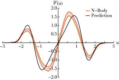
Figure 1: Illustration of the dimensionless flux, ${\overline{\mathcal{F}}(u,t\!=\!0)}$, as defined in Eq. (26) for the non-Gaussian PDF from Eq. (68) with ${\alpha=4}$, and an initial velocity dispersion given by ${\sigma=3}$. We recover a fairly good quantitative agreement between the measurements from direct $N$-body simulations (with the associated errors) and the prediction of the present kinetic theory (computed with ${k_{\mathrm{max}}=40}$, see Fig. 3), given that the latter is for hot systems only. Detailed parameters for these runs (${N\!=\!1024}$, ${\epsilon\!=\!0.01}$, and ${Q\!=\!9.75}$) are spelled out in Appendix C.

In that figure, we compare direct measurements from $N$-body simulations (following Appendix C) with the prediction from the kinetic equation (4) (using the well-posed rewriting from Eq. (46)). This figure shows a good quantitative agreement between the measured and the predicted fluxes. There are (at least) four possible origins for the slight mismatch observed in that figure. (i) There could be some remaining contributions stemming from collective effects, still present here for the value ${Q\simeq 9.75}$. (ii) There could be some non-vanishing contributions from the source term in ${G_{2}^{(1)}\!\times\!G_{2}^{(1)}}$ that was neglected in Appendix A when truncating the BBGKY evolution equations. (iii) Even with ${\epsilon=0.01}$, the ring model from Eq. (50) still corresponds to a quite hard and local interaction. As a result, the observed relaxation could still be partially driven by localised encounters (Chaffi et al., 2017). (iv) Finally, one cannot rule out that the numerical simulations could be partially flawed on such long integration times.

VII Conclusions

This paper presented the closed and explicit kinetic equation of discrete one-dimensional homogeneous long-range interacting systems with arbitrary pairwise couplings. This theory generalises the Landau kinetic equation for systems where the ${1/N}$ relaxation is blocked by symmetry and clarifies how three-body correlations can still drive very-long-term evolutions. This kinetic equation satisfies mass, momentum, energy conservation, and an $H$-theorem ensuring relaxation towards the Boltzmann equilibrium. Provided that the interaction is long-range, this equation cannot suffer any further kinetic blocking. As such, Eq. (4) represents the ultimate relaxation equation for classes of hot enough systems. Conversely, we have shown that strictly local interactions are kinetically blocked. We demonstrated why Eq. (4) is always well-posed, in spite of the appearance of a fourth order principal value. We illustrated how this equation quantitatively matches measurements from direct $N$-body simulations with an anharmonic interaction potential given by Eq. (50). As expected, the much weaker ${1/N^{2}}$ interaction leads to a much slower relaxation requiring very long-term integrations which we carried on GPUs. The CUDA code for these simulations is available on request.

Beyond the scope of this paper, it would clearly be of interest to generalise Eq. (4) to colder configurations, by taking into account collective polarisations. In particular, such a generalisation should cure the large-scale divergence of Eq. (4) that appears for the Coulombian interaction (see Section V). Similarly, the present theory could also be expanded to account for the source term in ${G_{2}^{(1)}\!\times\!G_{2}^{(1)}}$ (see Appendix A), that leads to higher order terms in the DF. Finally, one should also investigate the case of 1D inhomogeneous systems with monotonic frequency profiles, that can also suffer from kinetic blockings (see, e.g., Fouvry et al. (2019a)). Once these goals are reached, the kinetic theory of 1D discrete homogeneous long-range interacting systems will be completed.

Appendix A Deriving the kinetic equation

In this Appendix, we detail the key steps in the derivation of the kinetic equation (4). Notations and normalisations are the sames as the ones used in Fouvry et al. (2019b).

A.1 BBGKY hierarchy

The system is composed of $N$ identical particles of individual mass ${\mu=M_{\mathrm{tot}}/N}$. We write the phase space coordinates as ${\mathbf{w}=(\theta,v)}$. The instantaneous state of the system is characterised by its $N$-body PDF, ${P_{N}(\mathbf{w}_{1},...,\mathbf{w}_{N},t)}$, normalised as ${\!\int\!\mathrm{d}\mathbf{w}_{1}...\mathrm{d}\mathbf{w}_{N}P_{N}=1}$, and assumed to be symmetric w.r.t. any permutation of the particles. This PDF evolves according to Liouville’s equation

$$\frac{\partial P_{N}}{\partial t}+\big{[}P_{N},H_{N}\big{]}_{N}=0,$$ (51)

where the full $N$-body Hamiltonian reads

$$H_{N}(\mathbf{w}_{1},...,\mathbf{w}_{N})=\frac{1}{2}\sum_{i=1}^{N}v_{i}^{2}+\mu\sum_{i<j}^{N}U(\theta_{i}-\theta_{j}),$$ (52)

with ${U(\theta_{i}-\theta_{j})}$ the considered pairwise interaction. Equation (51) also involves the Poisson bracket over $N$ particles, that is defined with the convention

$$\big{[}P_{N},H_{N}\big{]}_{N}=\sum_{i=1}^{N}\bigg{(}\frac{\partial P_{N}}{\partial\theta_{i}}\frac{\partial H_{N}}{\partial v_{i}}-\frac{\partial P_{N}}{\partial v_{i}}\frac{\partial H_{N}}{\partial\theta_{i}}\bigg{)}.$$ (53)

In order to better capture the statistical structure of Eq. (51), we introduce the reduced DFs, $F_{n}$, defined as

$$F_{n}(\mathbf{w}_{1},...,\mathbf{w}_{n},t)=\mu^{n}\frac{N!}{(N-n)!}\!\!\int\!\!\mathrm{d}\mathbf{w}_{n+1}...\mathrm{d}\mathbf{w}_{N}\,P_{N}.$$ (54)

With such a choice, we highlight that one has ${\!\int\!\mathrm{d}\mathbf{w}F_{1}(\mathbf{w})=M_{\mathrm{tot}}}$, so that ${F_{1}\sim 1}$ w.r.t. $N$ the total number of particles. The definition from Eq. (51) allows us then to obtain the BBGKY hierarchy as

$$\frac{\partial F_{n}}{\partial t}+\big{[}F_{n},H_{n}\big{]}_{n}+\!\!\int\!\!\mathrm{d}\mathbf{w}_{n+1}\big{[}F_{n+1},\delta H_{n+1}\big{]}_{n}=0,$$ (55)

where we introduced ${\delta H_{n+1}}$ as the specific interaction energy of the $(n+1)^{\mathrm{th}}$ particle with the $n$ first. More precisely, it reads

$$\delta H_{n+1}(\mathbf{w}_{1},...,\mathbf{w}_{n+1})=\sum_{i=1}^{N}U(\theta_{i}-\theta_{n+1}).$$ (56)

The first three equations of the BBGKY hierarchy, i.e., the evolution equations for $F_{1}$, $F_{2}$, and $F_{3}$ are the starting points to derive the kinetic equation.

A.2 Cluster expansion

In order to perform a perturbative expansion of the evolution equations, the next stage of the calculation is to introduce the cluster expansion of the DFs, following the same normalisation as in Fouvry et al. (2019b).

As an example, we introduce the two-body correlation function as

$$F_{2}(\mathbf{w}_{1},\mathbf{w}_{2})=F_{1}(\mathbf{w}_{1})\,F_{1}(\mathbf{w}_{2})+G_{2}(\mathbf{w}_{1},\mathbf{w}_{2}).$$ (57)

Similar definitions are introduced for the three-body and four-body correlations functions, ${G_{3}}$ and $G_{4}$. We do not repeat their definitions here, but refer to Appendix B of Fouvry et al. (2019b).

In order to simplify the notations, we now write the one-body DF as ${F=F_{1}}$. The dynamical quantities at our disposal then satisfy the following scalings w.r.t. $N$: ${F\!\sim\!1}$, ${G_{2}\!\sim\!1/N}$, ${G_{3}\!\sim\!1/N^{2}}$, and ${G_{4}\!\sim\!1/N^{3}}$. As such, there are appropriate functions to perform perturbative expansions w.r.t. $N$.

The next step of the calculation is to inject this cluster expansion into the three first equations of the BBGKY hiearchy, as given by Eq. (55), so as to obtain evolution equations for ${\partial F/\partial t}$, ${\partial G_{2}/\partial t}$ and ${\partial G_{3}/\partial t}$. These calculations are cumbersome, and are performed in Fouvry et al. (2020). We do not reproduce here these generic equations that can also be found in Appendix B of Fouvry et al. (2019b).

A.3 Truncating the evolution equations

To continue the calculation, we may now truncate the three evolution equations at order ${1/N^{2}}$. At this stage, the main point is to note that the evolution equation for ${\partial F/\partial t}$ only involves ${G_{2}}$, whose norm scales like ${1/N}$. As a consequence, in order to derive an equation at order ${1/N^{2}}$, one has to account for the corrections at order ${1/N^{2}}$ that arise in $G_{2}$. Introducing explicitly the small parameter ${\epsilon=1/N}$, we therefore write

$$G_{2}=\epsilon\,G_{2}^{(1)}+\epsilon^{2}\,G_{2}^{(2)}.$$ (58)

Similarly, recalling the definition ${\mu=M_{\mathrm{tot}}/N}$, we can finally perform in the BBGKY equations the replacements

$$\mu\to\epsilon\,\mu,\;\;\;G_{3}\to\epsilon^{2}\,G_{3},\;\;\;G_{4}\to\epsilon^{3}\,G_{4}.$$ (59)

At this stage, we are now in a position to truncate the three first BBGKY equations by keeping only terms up to order $\epsilon^{2}$. Moreover, relying on the split from Eq. (58), we also split the evolution equation for ${\partial G_{2}/\partial t}$ to obtain one evolution equation for ${\partial G_{2}^{(1)}/\partial t}$ (of order ${1/N}$) and one for ${\partial G_{2}^{(2)}/\partial t}$ (of order ${1/N^{2}}$).

We can further simplify the evolution equations, by relying on our homogeneous assumptions, i.e., one has ${F=F(v,t)}$, independent of $\theta$. As a result, any term involving ${\partial F/\partial\theta}$ vanishes. Similarly, the mean field potential, ${\!\int\!\mathrm{d}\mathbf{w}_{2}\,F(\mathbf{w}_{2})U^{\prime}(\theta_{1}-\theta_{2})}$, also vanishes.

In order to ease the analytical derivation of the kinetic equation, we assume that the system is dynamically hot, so that the contributions from collective effects can be neglected. This assumption neglects any backreaction of a correlation onto the instantaneous potential within which it evolves. In a nutshell, it neglects integral terms of the form

$$\!\!\int\!\!\mathrm{d}\mathbf{w}_{3}\,G_{2}^{(1)}(\mathbf{w}_{2},\mathbf{w}_{3})\,U^{\prime}(\theta_{1}-\theta_{3})\to 0,$$ (60)

and similar terms for $G_{2}^{(2)}$ and $G_{3}$.

The last truncations and simplifications that we perform are as follows. First, in the evolution equation for ${\partial F/\partial t}$, we may neglect the source term in $G_{2}^{(1)}$ responsible for the usual ${1/N}$ Landau term, as it vanishes for 1D homogeneous systems. Second, in the evolution equation for ${\partial G_{2}^{(2)}/\partial t}$, we can neglect the source term in ${G_{2}^{(1)}}$, as it does not contribute to the kinetic equation (see Fouvry et al. (2020)). Finally, in the evolution equation for ${\partial G_{3}/\partial t}$, we can neglect, in the hot limit, the source term in ${G_{2}^{(1)}\!\times\!G_{2}^{(1)}}$ as its contribution is a factor ${1/Q}$ smaller than the source term in $G_{2}^{(2)}$.

All in all, as a result of these truncations, one obtains a set of four coupled differential equations that describe self-consistently the system’s dynamics at order ${1/N^{2}}$. We do not repeat here these equations which can be found in Appendix C of Fouvry et al. (2019b).

A.4 Solving the equations

The key property of the previous coupled evolution equations is that they form a closed and well-posed hierarchy of coupled partial differential equations. In particular, because we have neglected collective effects, there is no need to invert integral operators, so that the equations can be solved sequentially. As such, we first solve for the time evolution for ${G_{2}^{(1)}}$, then $G_{3}$, $G_{2}^{(2)}$, and finally $F$. At each stage of this calculation, the previous solution is used as a time-dependent source term in the next evolution equation.

In practice, to solve these equations we rely on Bogoliubov’s ansatz, i.e., we assume ${F(v,t)=\mathrm{cst.}}$ on the (dynamical) timescale over which correlations evolve. We also neglect transients associated with initial conditions, i.e., we solve the evolution equations with the initial conditions ${G_{2}^{(1)}(t\!=\!0)\!=\!0}$, and similarly for $G_{2}^{(2)}$ and $G_{3}$. Finally, in order to describe the process of phase mixing, we rely on the ${2\pi}$-periodicity of the angle coordinate, and Fourier expand any function depending on $\theta$, e.g., following Eq. (2) for the interaction potential.

Having obtained an explicit expression for the time-dependence of ${G_{2}^{(2)}(t)}$, we can now aim for the expression of the collision operator ${\partial F/\partial t}$. Relying once again on Bogoliubov’s ansatz, this amounts to taking the limit ${t\!\to\!+\infty}$ in ${G_{2}^{(2)}(t)}$. A typical time integral takes the form ${\!\int_{0}^{t}\!\mathrm{d}t_{1}\mathrm{e}^{-\mathrm{i}(t-t_{1})\omega}}$, where the frequency $\omega$ is a linear combination of velocities. Because we have solved three evolution equations sequentially, we can get up to three such integrals nested in one another, with partial derivatives w.r.t. velocities intertwined in them. To obtain the asymptotic time behaviour, we rely on the formula (see, e.g., Eq. (D2) of (Fouvry et al., 2019b))

$$\lim\limits_{t\to+\infty}\!\!\int_{0}^{t}\!\!\mathrm{d}t_{1}\,\mathrm{e}^{-\mathrm{i}(t-t_{1})\omega}=\pi\delta_{\mathrm{D}}(\omega)-\mathrm{i}\mathcal{P}\bigg{(}\frac{1}{\omega}\bigg{)},$$ (61)

with ${\delta_{\mathrm{D}}(\omega)}$ the Dirac delta, and ${\mathcal{P}(1/\omega)}$ the Cauchy principal value. It is only at this stage that we evaluate the intertwined gradients w.r.t. the velocities so that they only act on the Dirac deltas and the Cauchy principal values.

Following all these manipulations, we still have a kinetic equation involving hundreds of terms, and requiring further simplifications. This is the stage where the symbolic algebra system allows for an efficient manipulation of the formal expressions. The key steps of these manipulations are: (i) perform integrations by parts, so that all the $\delta_{\mathrm{D}}^{\prime}$ and $\delta_{\mathrm{D}}^{\prime\prime}$ are transformed into $\delta_{\mathrm{D}}$; (ii) use the scaling relations of $\delta_{\mathrm{D}}$ and $\mathcal{P}$ (and their derivatives), e.g., ${\delta_{\mathrm{D}}(\alpha\,x)=\delta_{\mathrm{D}}(x)/|\alpha|}$, to take out the Fourier wavenumbers as much as possible; (iii) perform appropriate relabellings of the dummy velocities and dummy wavenumbers, so that the sole resonance condition present is ${\delta_{\mathrm{D}}(k_{1}(v-v_{1})+k_{2}(v-v_{2}))}$, i.e., the same resonance condition as in Eq. (4); (iv) use the presence of the resonance condition, ${\delta_{\mathrm{D}}(k_{1}(v-v_{1})+k_{2}(v-v_{2}))}$, to make the replacements ${(v\!-\!v_{2})\to-(k_{1})/(k_{2})(v-v_{1})}$ and ${(v_{1}\!-\!v_{2})\to-(k_{1}\!+\!k_{2})/(k_{2})(v-v_{1})}$, so that the principal values are only expressed as functions of ${(v-v_{1})}$.

After all these cumbersome manipulations, which we automated using some custom grammar in Mathematica, one finally obtains the closed result from Eq. (4). All the details and functions used for these calculations can be found in Fouvry et al. (2020).

Appendix B Linear Response Theory

When deriving the kinetic equation (4), we had to neglect the contributions associated with collective effects. As a result, this equation only applies in dynamical hot systems, where the self-consistent amplification of collective effects is unimportant. Luckily the amplitude of this dressing of the perturbations is straightforward to estimate by solving the linear response theory of the system.

A systematic approach for that calculation is to rely on already well-established results regarding the linear stability of inhomogeneous long-range interacting systems. As detailed in Eq. (5.94) of Binney and Tremaine (2008), a system’s stability is generically governed by the response matrix

$$\widehat{\mathbf{M}}_{pq}(\omega)\!=\!2\pi\sum_{k}\!\!\int\!\!\mathrm{d}J\,\frac{k\,\partial F/\partial J}{\omega-k\Omega(J)}\,\psi^{(p)*}_{k}(J)\,\psi^{(q)}_{k}(J),$$ (62)

with ${(\theta,J)=(\theta,v)}$ the angle-action coordinates, and ${\Omega(J)=v}$ the orbital frequencies. In that expression, following the so-called matrix method (Kalnajs, 1976), we introduced a biorthogonal set of basis elements on which the pairwise interaction is decomposed. For the present system, the natural basis elements follow from the Fourier decomposition of the interaction, that can be written under the separable form

$$U(\theta_{1}-\theta_{2}) \,=-\sum_{p}\psi^{(p)}(\theta_{1})\,\psi^{(p)*}(\theta_{2}),$$

$$\psi^{(p)}(\theta) \,=\sqrt{U_{p}}\,\mathrm{e}^{\mathrm{i}p\theta}.$$ (63)

The Fourier transform of the basis elements is straightforward to compute. It is independent of the action $v$, and reads ${\psi^{(p)}_{k}=\delta_{p}^{k}\sqrt{U_{k}}}$. We may finally introduce the dielectric function, ${\bm{\varepsilon}=\mathbf{I}-\widehat{\mathbf{M}}}$, that is the matrix

$$\varepsilon_{pq}(\omega)=\delta_{p}^{q}\bigg{\{}1-2\pi U_{p}\!\!\int\!\!\mathrm{d}v\,\frac{p\,\partial F/\partial v}{\omega-pv}\bigg{\}}.$$ (64)

As expected for homogeneous systems, we recover that the dielectric matrix is diagonal, ${\varepsilon_{pq}(\omega)=\delta_{p}^{q}\,\varepsilon_{p}(\omega)}$, so that Fourier harmonics are independent from one another.

Using the same dedimensionalisation as in Eq. (25), we can rewrite the dielectric function as

$$\varepsilon_{k}(\overline{\omega})=1-\frac{\overline{U}_{k}}{Q}\!\!\int\!\!\mathrm{d}u\,\frac{k\,\partial\overline{F}/\partial u}{\overline{\omega}-ku},$$ (65)

with ${\overline{\omega}=\omega t_{\mathrm{d}}}$ a dimensionless frequency.

In the particular case where the system’s DF is single-humped, i.e., possesses a single maximum, and is also even, i.e., ${F(-v)=F(v)}$, so that the maximum is reached in ${v=0}$, one can even better characterise the system’s dielectric matrix. In that case, the DF is linearly stable if, and only if, ${\varepsilon_{k}(0)>0}$ for all $k$ (see, e.g., Fouvry et al. (2019b)). Following Eq. (65), and recalling that the rescaled coupling coefficient ${\overline{U}_{k}=U_{k}/U_{\mathrm{max}}}$ is such that ${|\overline{U}_{k}|\leq 1}$, the DF is linearly stable if, and only if, one has

$$Q>Q_{\mathrm{c}}=-\!\!\int\!\!\mathrm{d}u\,\frac{\partial\overline{F}/\partial u}{u}.$$ (66)

One can easily compute the stability limit $Q_{\mathrm{c}}$ for simple PDFs. In particular, for a Gaussian PDF, one finds ${Q_{\mathrm{c}}=1}$.

Appendix C Numerical simulations

Let us briefly detail the setup of our numerical simulations used to investigate the long-term relaxation of the Ring model. Following the Hamiltonian from Eq. (50), the equations of motion for particle $i$ reads

$$\frac{\mathrm{d}\theta_{i}}{\mathrm{d}t} \,=v_{i},$$

$$\frac{\mathrm{d}v_{i}}{\mathrm{d}t} \,=-\sum_{j=1}^{N}\frac{\mu}{2}\frac{\sin(\theta_{i}-\theta_{j})}{(1-\cos(\theta_{i}-\theta_{j})+\epsilon)^{3/2}}.$$ (67)

We note that in the expression of the acceleration, ${\mathrm{d}v_{i}/\mathrm{d}t}$, the sum runs over all particles including $i$. Including this self-interaction is fine here, because the interaction potential does not diverge at zero separation owing to the softening length, $\epsilon$. Proceeding in that fashion simplifies the numerical implementation.

Since the Hamiltonian from Eq. (50) is separable, one can easily devise symplectic integration schemes for that problem. In practice, we used the fourth-order symplectic integrator from Yoshida (1990), that requires only three (costly) force evaluations per timestep. However, we note that without any harmonic expansion of the interaction potential, the equations of motion from Eq. (67) truly form a $N$-body system, as the computation of each acceleration requires ${\mathcal{O}(N)}$ operations.

In order to accelerate the integration of that system, we followed an approach similar to Rocha Filho (2014), and implemented the computations on GPUs. In practice, simulations were run on NVIDIA V100 GPUs, with ${N=1024}$ particles per simulation, and ${N_{\mathrm{threads}}=N}$ threads per computation block, i.e., one thread per particle. For this particular GPU, we could run ${N_{\mathrm{blocks}}=80}$ independent realisations simultaneously on a given GPU. In total, we performed ${N_{\mathrm{runs}}=20}$ different batches of simulations, i.e., we had a total of ${1600}$ independent realisations to perform the ensemble average.

In the numerical implementation, the computation of the particles’ accelerations is by far the most numerically demanding task. To accelerate these evaluations, we focused on three main points. (i) First, in Eq. (67), the trigonometric functions ${\cos(\theta_{i}\!-\!\theta_{j})}$ and ${\sin(\theta_{i}-\theta_{j})}$ are expanded using duplications formulae, so that one only has to compute ${(\sin(\theta_{i}),\cos(\theta_{i}))}$ for every particle, using the instruction sincos. (ii) Second, these harmonic functions are pre-computed once per particle, and loaded in shared data array to allow for fast coalesced memory accesses for all the threads in the same computation block. (iii) Third, the computation of the force in Eq. (67) was further accelerated by using the instruction rsqrt(x) that allows for a fast computation of ${1/\sqrt{x}}$. With such parameters, integrating for one timestep required ${1.3\,\mathrm{ms}}$ of computation time.

In practice, we set the softening length to ${\epsilon=0.01}$, which imposes ${U_{\mathrm{max}}\simeq 0.92}$, as defined in Eq. (24). We used an integration time step equal to ${\delta t=1/(50\!\times\!\sigma)}$, that guaranteed a relative error in the total energy of the order of ${10^{-5}}$. Each realisation was integrated for a total of ${4\!\times\!10^{8}}$ timesteps, requiring about 6 days of computation per realisation.

We used the same initial conditions as in Fouvry et al. (2019b), given by a generalised Gaussian distribution following

$$P(v) \,=\frac{\alpha}{2}\,\frac{A(\alpha,\sigma)}{\Gamma(1/\alpha)}\,\exp\big{[}-(A(\alpha,\sigma)|v|)^{\alpha}\big{]},$$

$$A(\alpha,\sigma) \,=\frac{1}{\sigma}\,\bigg{(}\frac{\Gamma(3/\alpha)}{\Gamma(1/\alpha)}\bigg{)}^{1/2}.$$ (68)

This PDF is normalised so that ${\!\int\!\mathrm{d}vP(v)=1}$, is of zero mean, and of variance $\sigma^{2}$. The particular case ${\alpha=2}$ corresponds to the case of the Gaussian distribution, already introduced in Eq. (28), whose stability threshold, following Eq. (66), reads ${Q_{\mathrm{c}}=1}$. In practice, in the numerical simulations, we used the value ${\alpha=4}$, which corresponds to a less peaked PDF, and chose the initial velocity dispersion to be ${\sigma=3}$. Finally, assuming ${M_{\mathrm{tot}}=1}$, the stability parameter, $Q$, from Eq. (24) becomes ${Q\simeq 9.75}$, while the stability threshold is ${Q_{\mathrm{c}}\simeq 0.46}$ (see (Fouvry et al., 2019b)), i.e., the considered initial condition is linearly stable. To measure in Fig. 1 the diffusion flux and the associated errors (16% and 84% confidence levels), we followed the exact same procedure as detailed in Appendix F of Fouvry et al. (2019b). We do not repeat it here.

The kinetic equation (4) involves an infinite sum over $k_{1},k_{2}$. In pratice, one has to truncate these sums. To do so, we may truncate the interaction potential from Eq. (2), so that ${U_{k}=0}$ for ${|k|>k_{\mathrm{max}}}$. The effect of such a truncation on the pairwise force is illustrated in Fig. 2.

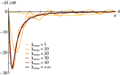
Figure 2: Illustration of the pairwise force, ${-\mathrm{d}U/\mathrm{d}\theta}$, as one varies the maximum index $k_{\mathrm{max}}$ considered in the interaction potential. As expected, the larger $k_{\mathrm{max}}$, the better the reconstruction of the exact interaction.

Doing so, we may then restrict the sums over fundamental resonances, as defined in Eq. (37), only to ${0<k,k^{\prime}\leq k_{\mathrm{max}}}$. Figure 3 illustrates the effect of $k_{\mathrm{max}}$ on the computed diffusion flux.

Figure 3: Illustration of the dependence of the dimensionless flux, ${\overline{\mathcal{F}}(u)}$, as one varies the maximum index ${k_{\mathrm{max}}}$ considered in the interaction potential. The considered system and initial conditions are identical to Fig. 1. As soon as the truncated Fourier series of $U_{k}$ represents accurately enough the underlying potential, ${U(\theta_{1}\!-\!\theta_{2})}$, the kinetic predictions have converged.

In that figure, we recover that for $k_{\mathrm{max}}$ large enough, the diffusion flux converges, so that higher order resonances do not contribute anymore to the relaxation. In practice, for the considered softening ${\epsilon=0.01}$, we used ${k_{\mathrm{max}}=40}$ in the predictions from Fig. 1.

References

- Campa et al. (2014) A. Campa et al., Physics of Long-Range Interacting Systems (Oxford Univ. Press, 2014).
- Nicholson (1992) D. R. Nicholson, Introduction to Plasma Theory (Krieger Publishing Company, Malabar, Florida, 1992).
- Binney and Tremaine (2008) J. Binney and S. Tremaine, Galactic Dynamics: Second Edition (Princeton Univ. Press, 2008).
- Chavanis (2002) P.-H. Chavanis, Statistical Mechanics of Two-Dimensional Vortices and Stellar Systems (Springer, Berlin, 2002), vol. 602, pp. 208–289.
- Bouchet and Venaille (2012) F. Bouchet and A. Venaille, Phys. Rep. 515, 227 (2012).
- Lynden-Bell (1967) D. Lynden-Bell, MNRAS 136, 101 (1967).
- Chavanis et al. (1996) P.-H. Chavanis, J. Sommeria, and R. Robert, ApJ 471, 385 (1996).
- Chavanis (2013a) P.-H. Chavanis, A&A 556, A93 (2013a).
- Chavanis (2013b) P.-H. Chavanis, Eur. Phys. J. Plus 128, 126 (2013b).
- Landau (1936) L. Landau, Phys. Z. Sowjetunion 10, 154 (1936).
- Boltzmann (1872) L. Boltzmann, Wien, Ber. 66, 275 (1872).
- Chandrasekhar (1943) S. Chandrasekhar, ApJ 97, 255 (1943).
- Rosenbluth et al. (1957) M. N. Rosenbluth, W. M. MacDonald, and D. L. Judd, Phys. Rev. 107, 1 (1957).
- Bogoliubov (1946) N. N. Bogoliubov, Problems of a Dynamical Theory in Statistical Physics (Moscow, 1946).
- Prigogine and Balescu (1959) I. Prigogine and R. Balescu, Physica 25, 281 (1959).
- Balescu (1960) R. Balescu, Phys. Fluids 3, 52 (1960).
- Lenard (1960) A. Lenard, Annals of Physics 10, 390 (1960).
- Klimontovich (1967) Y. L. Klimontovich, The Statistical Theory of Non-Equilibrium Processes in a Plasma (MIT press, Cambridge, 1967).
- Heyvaerts (2010) J. Heyvaerts, MNRAS 407, 355 (2010).
- Chavanis (2012a) P.-H. Chavanis, Physica A 391, 3680 (2012a).
- Fouvry et al. (2015) J.-B. Fouvry et al., A&A 584, A129 (2015).
- Fouvry et al. (2017) J.-B. Fouvry et al., MNRAS 471, 2642 (2017).
- Hamilton et al. (2018) C. Hamilton et al., MNRAS 481, 2041 (2018).
- Bar-Or and Fouvry (2018) B. Bar-Or and J.-B. Fouvry, ApJL 860, L23 (2018).
- Benetti and Marcos (2017) F. P. C. Benetti and B. Marcos, Phys. Rev. E 95, 022111 (2017).
- Chavanis (2012b) P.-H. Chavanis, Eur. Phys. J. Plus 127, 19 (2012b).
- Eldridge and Feix (1963) O. C. Eldridge and M. Feix, Phys. Fluids 6, 398 (1963).
- Dawson (1962) J. Dawson, Phys. Fluids 5, 445 (1962).
- Dawson (1964) J. M. Dawson, Phys. Fluids 7, 419 (1964).
- Rouet and Feix (1991) J. L. Rouet and M. R. Feix, Phys. Fluids 3, 1830 (1991).
- Dubin and O’Neil (1988) D. H. E. Dubin and T. M. O’Neil, Phys. Rev. Lett. 60, 1286 (1988).
- Chavanis (2001) P.-H. Chavanis, Phys. Rev. E 64, 026309 (2001).
- Dubin (2003) D. H. E. Dubin, Phys. Plasmas 10, 1338 (2003).
- Chavanis and Lemou (2007) P.-H. Chavanis and M. Lemou, Eur. Phys. J. B 59, 217 (2007).
- Chavanis (2012c) P.-H. Chavanis, Physica A 391, 3657 (2012c).
- Chavanis (2012d) P.-H. Chavanis, J. Stat. Mech. 2012, 02019 (2012d).
- Bouchet and Dauxois (2005) F. Bouchet and T. Dauxois, Phys. Rev. E 72, 045103 (2005).
- Chavanis et al. (2005) P.-H. Chavanis, J. Vatteville, and F. Bouchet, Eur. Phys. J. B 46, 61 (2005).
- Gupta and Mukamel (2011) S. Gupta and D. Mukamel, J. Stat. Mech. 2011, 03015 (2011).
- Barré and Gupta (2014) J. Barré and S. Gupta, J. Stat. Mech. 2014, 02017 (2014).
- Lourenço and Rocha Filho (2015) C. R. Lourenço and T. M. Rocha Filho, Phys. Rev. E 92, 012117 (2015).
- Fouvry et al. (2019a) J.-B. Fouvry, B. Bar-Or, and P.-H. Chavanis, Phys. Rev. E 99, 032101 (2019a).
- Yamaguchi et al. (2004) Y. Y. Yamaguchi et al., Physica A 337, 36 (2004).
- Rocha Filho et al. (2014a) T. M. Rocha Filho et al., Phys. Rev. E 89, 032116 (2014a).
- Rocha Filho et al. (2014b) T. M. Rocha Filho et al., Phys. Rev. E 90, 032133 (2014b).
- Fouvry et al. (2019b) J.-B. Fouvry, B. Bar-Or, and P.-H. Chavanis, Phys. Rev. E 100, 052142 (2019b).
- Campa et al. (2008) A. Campa et al., Phys. Rev. E 78, 040102 (2008).
- Fouvry et al. (2020) J.-B. Fouvry, P.-H. Chavanis, and C. Pichon, Mathematica notebook (2020).
- Balescu (1997) R. Balescu, Statistical Dynamics: Matter out of Equilibrium (Imperial Coll., London, 1997).
- Sota et al. (2001) Y. Sota et al., Phys. Rev. E 64, 056133 (2001).
- Rocha Filho (2014) T. M. Rocha Filho, Comput. Phys. Commun. 185, 1364 (2014).
- Chaffi et al. (2017) Y. Chaffi, T. M. Rocha Filho, and L. Brenig, arXiv 1711.07353 (2017).
- Kalnajs (1976) A. J. Kalnajs, ApJ 205, 745 (1976).
- Yoshida (1990) H. Yoshida, Phys. Lett. A 150, 262 (1990).