Money flow network among firms’ accounts
in a regional bank of Japan

Abstract

In this study, we investigate the flow of money among bank accounts possessed by firms in a region by employing an exhaustive list of all the bank transfers in a regional bank in Japan, to clarify how the network of money flow is related to the economic activities of the firms. The network statistics and structures are examined and shown to be similar to those of a nationwide production network. Specifically, the bowtie analysis indicates what we r efer to as a “walnut” structure with core and upstream/downstream components. To quantify the location of an individual account in the network, we used the Hodge decomposition method and found that the Hodge potential of the account has a significant correlation to its position in the bowtie structure as well as to its net flow of incoming and outgoing money and links, namely the net demand/supply of individual accounts. In addition, we used non-negative matrix factorization to identify important factors underlying the entire flow of money; it can be interpreted that these factors are associated with regional economic activities. One factor has a feature whereby the remittance source is localized to the largest city in the region, while the destination is scattered. The other factors correspond to the economic activities specific to different local places. This study serves as a basis for further investigation on the relationship between money flow and economic activities of firms.

Keywords: input-output table, Hodge decomposition, non-negative matrix factorization, walnut structure

RIKEN-iTHEMS-Report-20

Introduction

Determining how money flows among economic entities is an important aspect of understanding the underlying economic activities. For example, the so-called flow of funds accounts record the financial transactions and the resulting credits and liabilities among households, firms, banks, and the government (see, e.g., [1]). Another example is the input-output table, which describes the purchase and sale relationships among producers and consumers within an economy and clarifies the flows of final and intermediate goods and services with respect to industrial sectors and product outputs (e.g., [2]). These data are used in macroscopic studies, such as those of industrial sectors and aggregated economic entities.

Recent years have witnessed the increasing emergence of microscopic data. For example, one can study a nationwide production network, i.e., how individual firms transfer money among one another as suppliers and customers for transactions of goods and services (see [3] and the references therein). In contrast to the macroscopic studies mentioned above, microscopic studies can uncover the heterogeneous structure of the network and its role in economic activities, how the activities are subject to shocks due to natural disasters [4] and pandemics [5], and so forth. However, microscopic data are not exhaustive; although they may cover most active firms, not all the suppliers and customers are recorded. Such records are based on a survey in which a firm nominates a selected number of important customers and suppliers. In addition, the transaction amounts are often lacking; hence, the network is directed but only binary. More importantly, microscopic and macroscopic data are compiled and updated annually or quarterly at most (see [3, 6] and the references therein).

To uncover how economic entities such as firms perform economic activities in a real economy, we should ideally study how money flows among firms by using real-time data of bank transfers with exhaustive lists of accounts and transfers. To the best of our knowledge, such a study has not been conducted thus far, simply because such data are not available for academic purposes. The present study precisely performs such an analysis of a Japanese bank’s dataset. The bank is a regional bank, which has a high market share with respect to the loans and deposits in a prefecture, particularly supporting financial transactions among the manufacturing firms located there (according to a disclosure issued by the bank).

The objective of this study is to investigate economic activities via bank transfers among firms’ accounts by selecting all the transfers related to the firms to uncover how money flows behind the economic activities. More specifically, we examine the network and flow structures, especially the so-called bowtie structure, to locate the position of individual accounts upstream and downstream of the entire flow. We quantify the location using the method of Hodge decomposition of the flow. Furthermore, we find significant factors underlying the entire flow and interpret them using geographical information associated with the firms’ accounts.

Data

Our dataset comprises all the bank transfers that are sent from or received by the bank accounts in a regional bank. The regional bank is the largest bank in a prefecture in Japan (mid-sized in terms of its population (more than a million) and economic activity). Hereafter, we refer to it as Bank A for anonymity. The period covered in our study is from March 1, 2017, to July 31, 2019, i.e., a period of 29 months or 883 days.

During this period, there were 23 million transfers among 1.7 million bank accounts involving a total of 17.4 trillion yen (roughly 160 billion USD or 140 billion Euros). Let us denote a transfer from account $i$ to account $j$ by $i\rightarrow j$. To focus only on the firms’ accounts in Bank A, we filtered the data such that (i) both $i$ and $j$ are the accounts of Bank A, (ii) both $i$ and $j$ are owned by firms excluding households, and (iii) self-loops $i\rightarrow i$ are deleted. Point (ii) is important for our purpose, because our concern here is how money flows and circulates among firms’ accounts, which is considered to be closely related to the firms’ economic activities. The resulting data are summarized in Table 1 (see the rightmost column).

Table 1: Bank accounts and transfers: summary

Number/Amount	Entire data	Within Bank A
		all	firms
#Accounts	1.71 M	642,411	30,613
#Transfers	23.06 M	12,847,963	2,409,619
#Links	3.13 M	1,470,107	280,864
Transfer (Yen)	17.43 T	5.26 T	2.15 T

For a transfer $i\rightarrow j$, the column “Entire data” includes the cases in which either $i$ or $j$ is not an account of Bank A. The column “Within Bank A” corresponds to the case in which both $i$ and $j$ are accounts of Bank A. “firms” implies that both the source and the target of a link are firm accounts. M and T denote million and trillion, respectively.

Note that multiple transfers $i\rightarrow j$ can exist for a given pair of $i$ and $j$, because of frequent transfers. One can quantify the strength of the directional relationship between a pair of accounts either by the flow of transfers or by their frequency. To do so, we aggregate multiple transfers, if present, into a single link $i\rightarrow j$ with two types of weights, namely flow $f_{ij}$ and frequency $g_{ij}$ (see the illustration in Fig. 1). Hereafter, we use the term link for aggregated transfers.

The number of accounts or nodes in the network is $N=30,613$, while the number of links is $M=280,864$ after the aggregation (see Table 1).

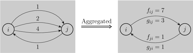
Figure 1: Construction of bank-transfer network by aggregation. How bank transfers are aggregated into links. $i$ made three transfers (1, 2, and 4) in an arbitrary unit of money to $j$, while $j$ made one transfer (1) to $i$ during a certain period. Flow $f_{ij}$ is defined by the total flow of transfers along $i\rightarrow j$. Frequency $g_{ij}$ is the frequency of these transfers.

The summary statistics of the links’ flows $f_{ij}$ and frequencies $g_{ij}$ for all the pairs of accounts $i$ and $j$ are presented in Table 2. One can observe that the distributions for flow and frequency have large skewness, implying that a considerable fraction of the money flow is due to a large amount transferred by a small number of flows.

Table 2: Summary statistics for links’ flows and frequencies

Stats.	Flow (Yen)	Frequency
Min.	1	1
Max.	$3.00\times 10^{10}$	2,616
Median	$0.20\times 10^{6}$	3
Avg.	$7.65\times 10^{6}$	8.58
Std.	$1.53\times 10^{8}$	19.92
Skewness	$92.5$	$37.8$
Kurtosis	$1.25\times 10^{4}$	$3.49\times 10^{3}$

Summary statistics of the links’ flows and frequencies for all the pairs of accounts, where links are aggregated transfers as defined in the main text and Fig. 1.

Results and Discussion

Network of firms’ accounts and links of transfers

First, let us summarize the network structure comprising firms’ accounts as nodes and aggregated transfers as links. We remark that transfers are aggregated into links as shown in Fig. 1. The degree is the number of transfers received by or sent from an account. The number of incoming and outgoing links of an account is called the in-degree and out-degree, respectively. Fig. 2 shows the distributions of the in-degree and out-degree as complementary cumulative distributions. By noting that the total number of accounts is $N=30,613$, we can see that a small fraction of accounts has a considerable degree, i.e., a thousand or more links, while most accounts have a limited number of links. Such hubs are presumably entities associated with the local government or the public sector in the region.

Because each node has an in-degree and out-degree, we can examine how they are correlated. Fig. 3 shows the scatter plot for the in-degree and out-degree of each account. We can observe a tendency for a positive correlation between the degrees (Pearson’s $r=0.303$ ($p<10^{-6}$); Kendall’s $\tau=0.164$ ($p<10^{-6}$)). We also observe that there are accounts that have many more incoming links than outgoing ones (and vice versa), which can be respectively considered as “sinks” and “sources” with respect to the money flow.

Figure 2: Degree distributions for the bank transfer network. Complementary cumulative distributions for in-degree and out-degree, which refer to the number of incoming and outgoing links, respectively, of each account.

Figure 3: Scatter plot for in-degree and out-degree of each account. Each account as a node, represented as a point, has incoming links and outgoing links, the numbers of which are represented by the horizontal and vertical axes, respectively. The diagonal line represents the locations where the in-degree and out-degree are equal.

We can observe each link’s weights, flow $f_{ij}$, and frequency $g_{ij}$ (see Fig. 1). Fig. 4 shows the complementary cumulative distribution for the flow along each link. The distribution is highly skewed; there exist a small number of links that have a large amount of flow exceeding a billion yen—likely important channels with large flows of money. Quantitatively, 0.1% of the links have flows larger than a billion yen.

Fig. 5 shows the complementary cumulative distribution for the frequency along each link. The steps at 30 and 60 on the horizontal axis are considered to correspond to transfers performed once or twice in each month (recall that the entire period includes 29 months). We can see that 0.1% of the links have frequencies of 500 or more corresponding to daily transfers on weekdays.

Figure 4: Distribution for the flows of links. Complementary cumulative distributions for the amount of money defined by $f_{ij}$ between each pair of accounts $i$ and $j$ (see Fig. 1).

Figure 5: Distribution for the frequencies of transfers. Complementary cumulative distributions for the frequency defined by $g_{ij}$ between each pair of accounts $i$ and $j$ (see Fig. 1). We can observe that there are frequency steps around 30 and 60, which are presumed as periodic transfers performed once or twice in each month (recall that the entire period includes 29 months).

Community analysis

Communities or clusters in a network are tightly knit groups with high intra-group density and low inter-group connectivity [7]. Community analysis is useful for understanding how a network has such heterogeneous structures. We adopt the widely used Infomap method [8, 9] to detect communities in our data.

The results are presented in Table 3. “Level” indicates the level of communities in a hierarchical tree of communities that are detected recursively (see [9]). The number of communities indicates how many communities are detected at the corresponding level. The label “irr. comm.” denotes irreducible communities that cannot be decomposed further to the next level of smaller communities in the hierarchical decomposition. For example, 143 of 164 communities at the first level are irreducible ones, whereas the rest of them are decomposed into 2,327 smaller communities at the next level, and so forth.

Table 3: Numbers of communities, irreducible communities, and accounts at each level of community analysis using Infomap

Level	#comm.	#irr. comm.	#accounts	Ration(%)
1	164	143	355	0.012
2	2,327	2,264	28,948	94.5
3	215	215	1,310	0.043
Total	—	2,621	30,613	100.0

Each level corresponds to the hierarchical level in the Infomap community analysis [9]. A community at a level can be decomposed at the next lower level (from top to bottom). If a community cannot be decomposed further, it is called an irreducible community. The numbers of irreducible communities are listed in the third column. The fourth column lists the numbers of accounts belonging to these irreducible communities at each level.

We find that most of the communities are at the second level because of the number of accounts, and that most of the accounts (94.5%) belong the second-level communities. In our previous study [10] on the application of hierarchical community analysis using Infomap to a large-scale production network, we showed that a relatively shallow hierarchy can be observed at the fifth level as the lowest level; in particular, most firms are included at the second level, exactly as we find here. This is not surprising, because our data on bank transfers among firms’ accounts should reflect a regional fraction of the entire production network on a nationwide scale. The finding here is interesting, because this implies a self-similar structure of the production network.

Fig. 6 shows the distribution of the sizes of irreducible communities at the lowest level that includes all the accounts. The size of a community is simply the number of nodes included in the community. The result indicates that the size of the communities is highly skewed over a few orders of magnitude. We note that there exist more than 10 communities with sizes exceeding 100, which correspond to important clusters of economic activities that depend on geographical sub-regions and industrial sectors. We shall discuss this issue in our analysis of non-negative matrix factorization later.

Figure 6: Distributions of the sizes of irreducible communities. Rank-size plot for the sizes of irreducible communities detected using the Infomap method at all the levels, where the ranks are in descending order of the size with the lowest rank equal to the total number of irreducible communities (see Table 3). The size of a community is simply the number of nodes included in the community.

Bowtie structure

With respect to the flow of money, the accounts can be located in a classification of the so-called bowtie structure, which was first adopted in the study of the Internet [11]. Nodes in a directed network can be classified into a giant weakly connected component (GSCC), its upstream side as the IN component, its downstream side as the OUT component, and the rest of the nodes that do not belong to any of GSCC, IN, and OUT. In general, they can be defined as follows.

GWCC

Giant weakly connected component: the largest connected component when viewed as an undirected graph. At least one undirected path exists for an arbitrary pair of nodes in the component.

GSCC

Giant strongly connected component: the largest connected component when viewed as a directed graph. At least one directed path exists for an arbitrary pair of nodes in the component.

IN

Nodes from which the GSCC is reached via directed paths.

OUT

Nodes that are reachable from the GSCC via directed paths.

TE

“Tendrils”: the rest of GWCC

Therefore, we have the components such that

$$\text{GWCC}=\text{GSCC}+\text{IN}+\text{OUT}+\text{TE}$$ (1)

For our data of the entire network with $N=30,613$ nodes and $M=280,864$ links, the GWCC component comprises 30,225 (99.0%) nodes and 280,598 (99.9%) links. The components of GSCC, IN, and OUT are summarized in Table 4. As can be seen, nearly 40% of the accounts are inside GSCC. Further, 15% of the accounts are in the upstream portion or IN, whereas 37% are in the downstream portion or OUT. These figures are very similar to those observed in the production network in Japan in a previous study [10].

The set of three components of GSCC, IN, and OUT is usually referred to as a “bowtie”; however, we find that the entire shape does not look like a “bowtie” but like a “walnut” in the sense that IN and OUT are two mutually disjoint thin skins enveloping the core of GSCC rather than two wings elongating from the center of a bowtie. In fact, by examining the shortest-path lengths from GSCC to IN or OUT, we can see that the accounts in the IN and OUT components are just a few steps away from GSCC as shown in Table 5. This feature is also similar to the production network on a nationwide scale (see the walnut structure in [10]); however, is different from many social and technological networks such as the Internet, where the maximum distances from GSCC to IN or OUT are usually very long (see the original paper [11]).

Table 4: Bowtie or “walnut” structure: size of each component.

Component	#accounts	Ratio(%)
GSCC	11,543	38.2%
IN	4,508	14.9%
OUT	11,270	37.3%
TE	2,904	9.6%
total	30,225	100%

“Ratio” refers to the ratio of the number of firms to the total number of accounts in GWCC.

Table 5: “Walnut” structure: shortest distance from GSCC to IN/OUT.

IN to GSCC			OUT from GSCC
Distance	#accounts	Ratio(%)	Distance	#accounts	Ratio(%)
1	4,346	96.41%	1	11,051	98.06%
2	144	3.19%	2	208	1.85%
3	8	0.18%	3	11	0.10%
4	10	0.22%	4	0	0.00%
Total	4,508	100%	Total	11,270	100%

The left half lists the number of accounts in the IN component connected to the GSCC accounts with the shortest distances within 4 at most. The right half represents the OUT component similarly.

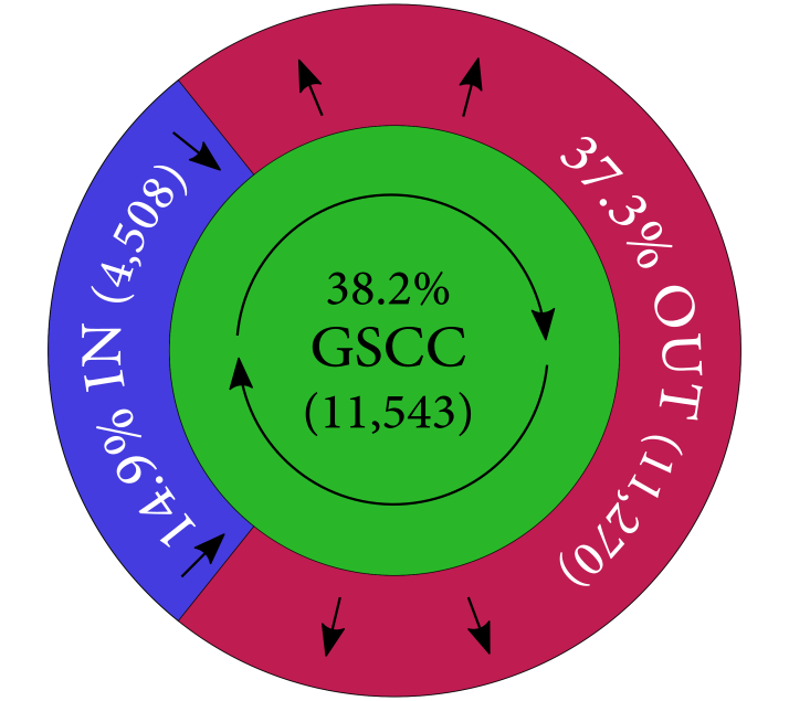
Figure 7: Walnut structure: a schematic view. The so-called bowtie structure reveals that GSCC includes nearly 40% of all the nodes or accounts, while the IN and OUT components include 15% and 37%, respectively (see Table 4 for the details). The prominent features are as follows. (i) The shortest distances to IN and OUT from GSCC are quite small, typically 1 or 2, and 4 at most (Table 5); hence, the ties are not elongated like a “bowtie” but rather like a “walnut” skin. (ii) The nodes in the components of IN and OUT are connected to the nodes scattered widely in GSCC. See also the study of a supplier-customer network [10] with similar features.

Hodge decomposition: upstream/downstream flow

Our analysis of the bowtie structure implies that the nodes in IN and OUT are located in the upstream and downstream sides in the flow of money. The Hodge decomposition of the flow in a network is a mathematical method of ranking nodes according to their locations upstream or downstream of the flow [12]. This method, also known as the Helmholtz–Hodge–Kodaira decomposition, has been used to find such a structure in complex networks (see, e.g., neural networks [13] and economic networks [14, 15, 16]).

First, we recapitulate the method in a manner suitable for our purpose here. Let $A_{ij}$ denote adjacency matrix of our directed network of bank transfers, i.e.,

$$A_{ij} =\begin{cases}1&\text{if there is a link of transfer from account $i$ to $j$},\\ 0&\text{otherwise}.\end{cases}$$ (2)

Recall that the numbers of accounts and links are $N$ and $M$, respectively. We excluded all the self-loops, implying that $A_{ii}=0$. Each link has a flow, denoted by $B_{ij}$, either of the total amount of transfers, $f_{ij}$, or the frequency of transfers, $g_{ij}$ (see Fig. 1), i.e.,

$$B_{ij} =\begin{cases}f_{ij}\text{ or }g_{ij}&\text{if there is a flow from $i$ to $j$},\\ 0&\text{otherwise}.\end{cases}$$ (3)

Note that there may be a pair of accounts such that $A_{ij}=A_{ji}=1$ and $B_{ij},B_{ji}>0$. Next, we shall take the frequency of transfers, $g_{ij}$, by assuming that it represents the strength of the link.

Let us define a “net flow” $F_{ij}$ by

$$F_{ij}=B_{ij}-B_{ji}$$ (4)

and a “net weight” $w_{ij}$ by

$$w_{ij}=A_{ij}+A_{ji}.$$ (5)

Note that $w_{ij}$ is symmetric, i.e., $w_{ij}=w_{ji}$, and non-negative, i.e., $w_{ij}\geq 0$ for any pair of $i$ and $j$. We remark that Eq. (5) is simply a convention to consider the effect of mutual links between $i$ and $j$. One could multiply Eq. (5) by 0.5 or an arbitrary positive number, which does not change the result significantly for a large network.

Now, the Hodge decomposition is given by

$$F_{ij}=F^{(\text{c})}_{ij}+F^{(\text{g})}_{ij},$$ (6)

where the circular flow $F^{(\text{c})}_{ij}$ satisfies

$$\sum_{j}F^{(\text{c})}_{ij}=0,$$ (7)

which implies that the circular flow is divergence-free. The gradient flow $F^{(\text{g})}_{ij}$ can be expressed as

$$F^{(\text{g})}_{ij}=w_{ij}(\phi_{i}-\phi_{j}),$$ (8)

i.e., the difference of “potentials”. In this manner, the weight $w_{ij}$ serves to make the gradient flow possible only where a link exists. We refer to the quantity $\phi_{i}$ as the Hodge potential. If $\phi_{i}$ is relatively large, the account $i$ is located in the upstream side of the entire network, while a small $\phi_{i}$ implies that $i$ is located in the downstream side of the entire network.

Eqs. (6)–(8) can be solved as follows. First, we combine them into the following equation for the Hodge potentials $(\phi_{1},\cdots,\phi_{N})(\equiv\bm{\phi})$:

$$\sum_{j}L_{ij}\phi_{j}=\sum_{j}F_{ij}\ ,$$ (9)

for $i=1,\ldots,N$. Here, $L_{ij}$ is the so-called graph Laplacian and defined by

$$L_{ij}=\delta_{ij}\sum_{k}w_{ik}-w_{ij}\ ,$$ (10)

where $\delta_{ij}$ is the Kronecker delta.

It is straightforward to show that the matrix $L=(L_{ij})$ has only one zero mode (eigenvector with zero eigenvalue), i.e., $\bm{\phi}=(1,1,\cdots,1)/\sqrt{N}$. The presence of this zero mode simply corresponds to the arbitrariness in the origin of $\phi$. We can show that all the other eigenvalues are positive (see, e.g., [17]). Therefore, Eq. (9) can be solved for the potentials by fixing the potentials’ origin. We assume that the average value of $\phi$ is zero, i.e., $\sum_{i}\phi_{i}=0$.

The Hodge potentials obtained for the entire network of GWCC are shown in Fig. 8 as the distribution for the potentials of all the accounts in GWCC (red line). By noting that the average is zero by definition, we can see that it is a bimodal distribution with two peaks at positive and negative values, while there are a number of potential values close to zero (peaks around zero). The nodes in TE (tendrils) can be considered to have locations that are not particularly relevant to upstream or downstream; we can expect that these nodes mostly have potentials close to zero, as shown by the blue line, i.e., the result after deleting all the nodes contained in TE’s. We can see that these TE do not contribute to large absolute values of the Hodge potentials.

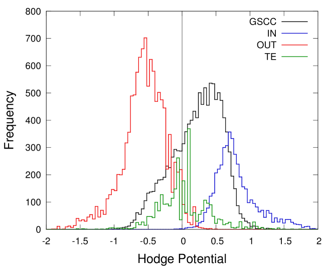
Figure 8: Distribution of the Hodge potentials of individual accounts. Distributions as histograms of $\phi_{i}$ in each component of the bowtie or walnut structure Fig. 7. The horizontal axis represents the value of $\phi_{i}$ of an individual node or account, while the vertical axis represents the frequency in the histogram. The black line corresponds to GSCC or the core. The blue and red lines, respectively, correspond to the IN and OUT components or upstream and downstream with respect to the core. The green line corresponds to TE (tendrils) or the rest of the nodes.

It can be expected that there is a correlation between the value of the Hodge potential and the net amount of demand or supply of money for each node. We can measure the net amount of demand/supply by examining the in-degree and out-degree of the node, or alternatively, the in-flow and out-flow of money. Fig. 9 and Fig. 10 show the results. We find that if the potential is positive, the node is located in the upstream side, and its net degree and flow are negative. If the potential is negative, the node is located in the downstream side, and its net degree and flow are positive.

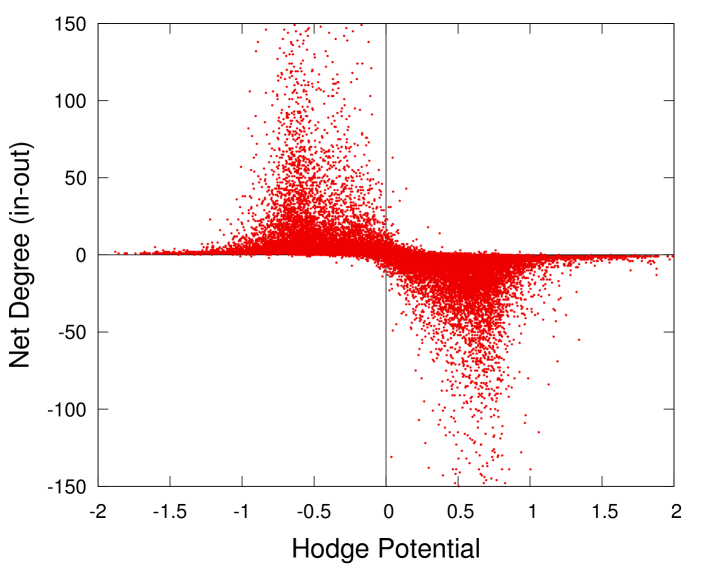
Figure 9: Hodge potential and net degree for each node. Each point represents a node or an account. The net degree is defined by the difference between the in-degree and the out-degree of the node. If the net degree is positive, the node has more incoming links than outgoing ones and vice versa.

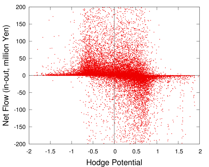
Figure 10: Hodge potential and net flow for each node. This figure is similar to Fig. 9 except for the vertical axis, which represents the net flow. The net flow is defined by the difference between the incoming amount of money and the outgoing one.

This finding can be interpreted as follows. Consider a supplier in the production network, which supplies its products to a number of customers. The supplier has a bank account (or possibly multiple accounts) that receives money from the customers’ accounts as the supplier’s sales. If the supplier is in the upstream side of the supplier-customer relationship, it is likely that the account is located in the downstream side of the money flows in this study. As the supplier not only makes sales but also incurs costs, typically labor costs, there must be an outgoing flow from its account to be linked with households and other non-commercial entities, which are not included in the present study. Consequently, the supplier’s account has a negative net degree and flow, while its Hodge potential is likely positive. A similar argument would hold for customers in an opposite way. In other words, our finding is a direct observation of how the flow of money reflects the economic activities among the firms’ accounts.

Non-negative matrix factorization (NMF): hidden factors of flows

We would like to show that there are hidden “factors” in the entire flow of the network. By “factor”, we mean a component that can explain a significant part of the flow. Alternatively, the entire flow can be decomposed into only a small number of factors.

In this section, we focus on the geographical information of bank transfers. Each bank account has an address. We obtain the latitudes and longitudes of the bank accounts by using geocoding. Consequently, a bank transfer between two bank accounts has two coordinates of its remittance source and destination. We construct a non-negative matrix defined from the frequencies between the geographical areas, and we adopt NMF to find the hidden factors of geographical structures of the flow.

NMF constructs an approximate factorization of a non-negative matrix [18]. For example, NMF is useful for processing facial images because it produces parts-based representations of such images [19]. To reveal the basic components of the geographical structure of bank transfers, we apply NMF to a non-negative matrix $V=(V_{mn})$ defined as follows. We set a square area including the prefecture and split it into $K\times K$ smaller squares in a lattice pattern, where $K=100$. Let $R_{pq}$ be the $(p,q)$ small square area for $1\leq p,q\leq K$. We consider the frequencies of bank transfers between two small square areas. Let $\alpha(p_{1},q_{1},p_{2},q_{2})$ be the frequency of bank transfers from $(p_{1},q_{1})$ to $(p_{2},q_{2})$ for $1\leq p_{1},q_{1},p_{2},q_{2}\leq K$, i.e., using the frequency $g_{ij}$ of transfers from account $i$ to account $j$,

$$\alpha(p_{1},q_{1},p_{2},q_{2})=\sum_{\{(i,j)\mid(x_{i},y_{i})\in R_{p_{1}q_{1}},(x_{j},y_{j})\in R_{p_{2}q_{2}}\}}g_{ij},$$ (11)

where $(x_{i},y_{i})$ is the coordinate of the address of account $i$. The non-negative matrix $V$ of size $K^{2}\times K^{2}$ is defined by

$$V_{mn}=\log(\max\{1,\alpha(p_{1},q_{1},p_{2},q_{2})\}),$$ (12)

where $m=p_{1}+(q_{1}-1)K$ and $n=p_{2}+(q_{2}-1)K$. For practical purposes, we convert the frequencies into their logarithmic values to reduce the influence of outstanding values.

NMF gives the approximate factorization

$$V\approx WH$$ (13)

for some integer $d$, where $W$ and $H$ are non-negative matrices of size $K\times d$ and $d\times K$, respectively. We let $d=10$ from prior knowledge that the number of local communities in the prefecture is around 10. Since the $m$th row of $V$ corresponds to bank transfers from $(p,q)$ for $m=p+(q-1)K$, the rows of $H$ constitute a basis of bank transfers for the given sources. Similarly, since the $m$th column corresponds to bank transfers to $(p,q)$ for $m=p+(q-1)K$, the columns of $W$ constitute a basis of bank transfers for the given destinations. We can regard Eq. (13) as the approximation of $V$ by the sum of products of these basis vectors. By letting $w_{m}$ be the $m$th column vector and $h_{m}$ be the $m$th row vector, we have

$$V \approx\sum_{m=1}^{d}w_{m}h_{m}.$$ (14)

The logarithms of the frequencies of bank transfers in the target area are decomposed into matrices $w_{m}h_{m}$ for $m=1,\dots,d$.

A basis vector $v$, which is a column vector $w_{m}$ of $W$ or a row vector $h_{m}$ of $H$, can be converted to a $K\times K$ matrix $D(v)$, $1\leq p,q\leq K$, on the geographical square area because an entry of $V$ corresponds to the frequency of bank transfers between two small square areas. In other words, $D(v)$ is represented as a heatmap in the geographical area and Fig. 11 shows a heatmap of a basis vector. Since basis vectors seem to indicate geographically localized structures, to quantify such structures, we consider a circular area for a basis vector so that the sum of entries of the basis vector included in the circular area is maximized. Let $r_{pq}$ be the coordinate of the center of $R_{pq}$ and let $C_{pq}$ be a circular area whose radius is 10 km and center is $r_{pq}$. For a $K\times K$ matrix $E=(E_{pq})$ and a circular area $C$, we define

$$\beta(C,E) =\frac{\sum_{\{(p,q)\mid r_{pq}\in C\}}E_{pq}}{\sum_{\{(p,q)\mid 1\leq p,q\leq K\}}E_{pq}}.$$ (15)

The proportion $\gamma(v)$ is calculated by

$$C^{\prime}(v) =\mathop{\rm arg~{}max}\limits_{\{C_{pq}\mid 1\leq p,q\leq K\}}\beta(C_{pq},D(v))$$ (16)

$$\gamma(v) =\max_{\{C_{pq}\mid 1\leq p,q\leq K\}}\beta(C_{pq},D(v)).$$ (17)

The proportion $\gamma$ and the circular area $C^{\prime}$ of a basis vector are shown in Fig. 11.

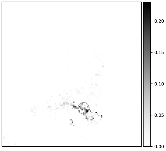
Figure 11: Normalized basis vector obtained by NMF. The circular area has the largest sum of entries of the basis vector included in the circular area. A normalized basis vector such that the sum of entries is one is converted into a heatmap whose lattice pattern corresponds to $R_{pq}$. The radius of the circular area is 10 km. The circular area is $C^{\prime}(v)$ for some basis vector $v$, i.e., it is located at a position such that $\beta(\cdot,D(v))$ is maximized.

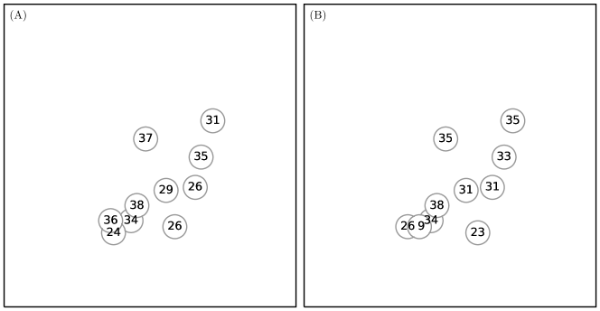
Figure 12: Circular areas corresponding to the basis vectors and proportions of the vector entries included in the circular areas. (A) is drawn from $w_{m}$, i.e., the basis vectors for sources, and the proportions $\gamma(w_{m})$, while (B) is drawn from $h_{m}$, i.e., the basis vectors for destinations, and the proportions $\gamma(h_{m})$ for $m=1,\dots,d$.

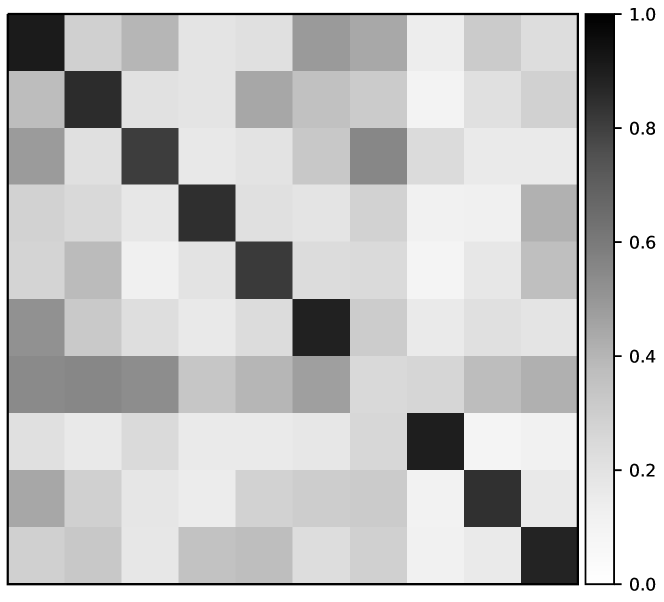
Figure 13: Cosine similarities between basis vectors. The vertical axis represents the indices of $h_{s}$, i.e., the $s$th row vector of $H$, and the horizontal axis represents the indices of $w_{t}$, i.e., the $t$th column vector of $W$. The index of the top left square is $(s,t)=(0,0)$.

The panels (A) and (B) in Fig. 12 show the proportions $\gamma$ of all the basis vectors of sources and destinations. The proportions are more than 23% except for one basis vector in both panels of the source and destination; therefore, most basis vectors of bank transfers are localized geographically. Since the positions of the circular areas are around the centers of cities, geographically localized properties are thought to reflect the economic activity in local areas.

Fig. 12 suggests that the basis vectors of the source and destination are similar to each other. To clarify this, Fig. 13 shows a matrix of cosine similarities between a basis vector of the source and a basis vector of the destination, where the cosine similarity of $w_{m}$ and $h_{n}$ is calculated by

$$\frac{w_{m}\cdot h_{n}}{\|w_{m}\|\|h_{n}\|},$$ (18)

where $w_{m}\cdot h_{n}$ is the inner product of $w_{m}$ and $h_{n}$ and $\|\cdot\|$ is the Euclidean norm of a vector. All the diagonal entries except for one are 1’s, i.e., the $m$th basis vector $h_{m}$ is similar to the $m$th basis vector $w_{m}$ except for $m=7$. These basis vectors correspond to basis vectors having geographically localized properties in Fig. 12, and the similarities of pairs of basis vectors imply that both incoming and outgoing bank transfers for a local area have similar patterns.

We can also interpret the seventh basis vectors of the source and destination that do not have similarities. The seventh basis vector of the source is localized to the largest city in the prefecture and the seventh basis vector of the destination is scattered throughout the prefecture. This means that the pair of these basis vectors corresponds to bank transfers from the largest city to the local areas. Therefore, Eq. (14) for our data gives decompositions that describe bank transfers in local areas and bank transfers between the largest city and local areas.

Finally, we state the results of NMF with different values of $d$. To investigate the changes in the basis vectors that occur according to $d$, we apply NMF to $V$ with $d=5,\dots,15$. In all the cases, most of the basis vectors are geographically localized and form source and destination pairs that are similar to each other and correspond to bank transfers in local areas. All the basis vectors are localized for $d$ less than 7, and there is a pair of basis vectors corresponding to bank transfers between the largest city and local areas for $d$ greater than or equal to 7. For all the values of $d$ that we have examined, the basis vectors correspond to either bank transfers in local areas or bank transfers between the largest city and other local areas.

Conclusion

We studied an exhaustive list of bank accounts of firms and remittances from source to destination within a regional bank with a high market share of loans and deposits in a prefecture of Japan. By studying such a network of money flow, we could uncover how firms conduct the underlying economic activities as suppliers and customers from the upstream side to the downstream side of the money flow. We aggregated the remittances that occurred for each pair of accounts as a link during the period from March 2017 to July 2019 (i.e., approximately two and a half years), which comprises 30K nodes and 0.28M links. We found that the statistical features of the network are actually similar to those of a production network on a nationwide scale in Japan [3], but with greater emphasis on the regional aspects.

The bowtie analysis revealed what we refer to as a “walnut” structure in which the core and upstream/downstream components are tightly connected within the shortest distances, typically at a few steps. By quantifying the location of the individual account of a firm using the method of Hodge decomposition, we found that the Hodge potential of each node can describe the location in the entire flow of money from the upstream side to the downstream side, well characterized by the values of the potential. In particular, there is a significant correlation between the Hodge potentials and the net flows of incoming and outgoing money and links as well as the potentials and the walnut structure. This implies that we can characterize the net demand/supply of each node and decompose the flows into those due to the difference in potentials as well as divergence-free flows. Furthermore, by using non-negative matrix factorization, we uncovered the fact that the entire flow can be considered as a combination of several significant factors. One factor has a feature whereby the remittance source is localized to the largest city in the region, while the destination is scattered. The other factors correspond to the economic activities specific to different local places, which can be interpreted as local activities of the economy.

We can consider several points that remain to be studied separately from the present work. While we aggregated the entire period in this paper, it would be interesting to determine how the network changes with time by examining the time-stamps recorded in every remittance. At time scales of days, weeks, and months, it is quite likely that there are intra-day, weekly, and seasonal patterns of activities. More interestingly, under mild changes in the booms and busts of the regional economy on a relatively long time scale, the economic agents might change their behaviors possibly by changing peers in the transactions. Alternatively, under sudden changes due to natural disasters or pandemics, the agents can change their usual patterns abruptly. In other words, these are important aspects of a temporally changing network.

In addition, further investigation of the aspect of money flow amounts is warranted in the sense that the dominant driving force likely comes from “giant players” who demand or supply a large amount of money. Moreover, it would be interesting to select them in a subgraph by choosing only links with flow amounts that are larger than a certain threshold. These topics will be studied in our future work.

Funding

This work was supported in part by MEXT as Exploratory Challenges on Post-K computer (Studies of Multi-level Spatiotemporal Simulation of Socioeconomic Phenomena), the project “Large-scale Simulation and Analysis of Economic Network for Macro Prudential Policy” undertaken at the Research Institute of Economy, Trade and Industry (RIETI), and JSPS KAKENHI Grant Numbers 17H02041, 19K22032, and 20H02391.

Availability of data and materials

The dataset is available in a collaborative scheme upon request to TT and YF at Shiga University.

Competing interests

The authors declare that they have no competing interests.

Author’s contributions

All authors contributed equally. All authors read and approved the final manuscript.

References

- [1] Bank of Japan: Guide to Japan’s Flow of Funds Accounts. https://www.boj.or.jp/en/statistics/. accessed June 2020
- [2] OECD: Input-Output Tables. http://www.oecd.org/sti/ind/input-outputtables.htm. accessed June 2020
- [3] Aoyama, H., Fujiwara, Y., Ikeda, Y., Iyetomi, H., Souma, W., Yoshikawa, H.: Macro-Econophysics – New Studies on Economic Networks and Synchronization. Cambridge University Press, Cambridge, UK (2017)
- [4] Inoue, H., Todo, Y.: Firm-level propagation of shocks through supply-chain networks. Nature Sustainability 2, 841–847 (2019)
- [5] Inoue, H., Todo, Y.: The Propagation of Economic Impacts through Supply Chains: The Case of a Mega-city Lockdown to Prevent the Spread of COVID-19. Research Institute of Economy, Trade and Industry (RIETI) Discussion Paper Series (2020)
- [6] Fujiwara, Y., Aoyama, H.: Large-scale structure of a nation-wide production network. The European Physical Journal B 77(4), 565–580 (2010)
- [7] Barabási, A.-L.: Network Science. Cambridge University Press, Cambridge, UK (2016)
- [8] Rosvall, M., Bergstrom, C.T.: Maps of random walks on complex networks reveal community structure. Proceedings of the National Academy of Sciences 105(4), 1118–1123 (2008)
- [9] Rosvall, M., Bergstrom, C.T.: Multilevel compression of random walks on networks reveals hierarchical organization in large integrated systems. PloS one 6(4), 18209 (2011)
- [10] Chakraborty, A., Kichikawa, Y., Iino, T., Iyetomi, H., Inoue, H., Fujiwara, Y., Aoyama, H.: Hierarchical communities in walnut structure of japanese production network. PLoS ONE 13(8), 10–13710202739 (2018)
- [11] Broder, A., Kumar, R., Maghoul, F., Raghavan, P., Rajagopalan, S., Stata, R., Tomkins, A., Wiener, J.: Graph structure in the Web. Computer Networks 33(1-6), 309–320 (2000)
- [12] Jiang, X., Lim, L.-H., Yao, Y., Ye, Y.: Statistical ranking and combinatorial hodge theory. Mathematical Programming 127(1), 203–244 (2011)
- [13] Miura, K., Aoki, T.: Scaling of hodge-kodaira decomposition distinguishes learning rules of neural networks. IFAC-PapersOnLine 48(18), 175–180 (2015). 4th IFAC Conference on Analysis and Control of Chaotic Systems CHAOS 2015
- [14] Kichikawa, Y., Iyetomi, H., Iino, T., Inoue, H.: Hierarchical and Circular Flow Structure of Interfirm Transaction Networks in Japan. https://ssrn.com/abstract=3173955 (2018)
- [15] Iyetomi, H., Aoyama, H., Fujiwara, Y., Souma, W., Vodenska, I., Yoshikawa, H.: Relationship between macroeconomic indicators and economic cycles in u.s. Sci. Rep. 10, 8420 (2020). https://doi.org/10.1038/s41598-020-65002-3
- [16] MacKay, R., Johnson, S., Sansom, B.: How directed is a directed network? arXiv preprint arXiv:2001.05173 (2020)
- [17] Fujiwara, Y., Islam, R.: Hodge Decomposition of Bitcoin Money Flow. Springer. in press (2020)
- [18] Lee, D.D., Seung, H.S.: Algorithms for non-negative matrix factorization. In: Proceedings of the 13th International Conference on Neural Information Processing Systems. NIPS’00, pp. 535–541. MIT Press, Cambridge, MA, USA (2000)
- [19] Lee, D.D., Seung, H.S.: Learning the parts of objects by non-negative matrix factorization. Nature 401(6755), 788–791 (1999). doi:10.1038/44565