Solving Phase Retrieval with a Learned Reference

Abstract

Fourier phase retrieval is a classical problem that deals with the recovery of an image from the amplitude measurements of its Fourier coefficients. Conventional methods solve this problem via iterative (alternating) minimization by leveraging some prior knowledge about the structure of the unknown image. The inherent ambiguities about shift and flip in the Fourier measurements make this problem especially difficult; and most of the existing methods use several random restarts with different permutations. In this paper, we assume that a known (learned) reference is added to the signal before capturing the Fourier amplitude measurements. Our method is inspired by the principle of adding a reference signal in holography. To recover the signal, we implement an iterative phase retrieval method as an unrolled network. Then we use back propagation to learn the reference that provides us the best reconstruction for a fixed number of phase retrieval iterations. We performed a number of simulations on a variety of datasets under different conditions and found that our proposed method for phase retrieval via unrolled network and learned reference provides near-perfect recovery at fixed (small) computational cost. We compared our method with standard Fourier phase retrieval methods and observed significant performance enhancement using the learned reference.

1 Introduction

The problem of phase retrieval refers to the challenge of recovering a real- or complex-valued signal from its amplitude measurements. This problem arises in diffraction imaging, X-ray crystallography, and ptychography [14, 15, 21, 35, 43]. Fourier phase retrieval is a special class of phase retrieval problems aimed at the recovery of a signal from the amplitude of its Fourier coefficients. Let us assume that Fourier amplitude measurements are given as

$$y=|Fx|+\eta,$$ (1)

where $F$ denotes the Fourier transform operator, $x$ denotes the unknown signal or image, and $\eta$ denotes the measurement noise. Our goal is to recover $x$ given $y$.

Fourier phase retrieval is essential in many applications, especially in optical coherent imaging. Classical methods for phase retrieval utilize the prior knowledge about the support and positivity of the signals [14, 15]. Subsequent work has considered the case where the unknown signal is structured and belongs to a low-dimensional manifold that is known a priori. Examples of such low-dimensional structures include sparsity [46, 27], low-rank [26, 12], or neural generative models [25, 28]. Other techniques like Amplitude flow [47] and Wirtinger flow use alternating minimization [7]. Many of these newer algorithms involve solving a non-convex problem using iterative, gradient-based methods; therefore, they need to be carefully initialized. The initialization technique of choice is spectral initialization, first proposed in the context of phase retrieval in [36], and extended to the sparse signal case in [46, 27].

Fourier phase retrieval problem does not satisfy the assumptions needed for successful spectral initialization and remains highly sensitive to the initialization choice. Furthermore, Fourier amplitude measurements have the so-called trivial ambiguities about possible shifts and flips of the images. Therefore, many Fourier phase retrieval methods test a number of random initializations with all possible flips and shifts and select the estimate with the best recovery error [34].

In this paper, we assume that a known (learned) reference is added to the signal before capturing the Fourier amplitude measurements. The main motivation for this comes from the empirical observation that knowing a part of the image can often help resolve the trivial ambiguities [3, 18, 22]. We extend this concept and assume that a known reference signal is added to the target signal and aim to recover the target signal from the Fourier amplitude of the combined signal. Adding a reference may not feasible in all cases, but our method will be applicable whenever we can add a reference or split the target signal into known and unknown parts. We can describe the Fourier amplitude (phaseless) measurements with a known reference signal $u$ as

$$y=|F(x+u)|+\eta.$$ (2)

Similar reference-based measurements and phase retrieval problems also arise in holographic optical coherence imaging [37].

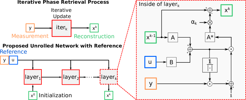
Our goal is to recover the signal $x$ from the amplitude measurements in (2). To do that, we implement a gradient descent method for phase retrieval. We present the algorithm as an unrolled network for a general system in Fig. 1. Every layer of the network implements one step of the gradient descent update. To minimize the computational complexity of the recovery algorithm, we seek to minimize the number of iterations (hence the layers in the network). In addition, we seek to learn the reference $u$ to maximize the accuracy of the recovered signal for a given number of iterations. The learned $u$ and reconstruction results for different datasets are summarized in Fig. 2.

1.1 Our Contributions

We present an iterative method to efficiently recover a signal from the Fourier amplitude measurements using a fixed number of iterations. To achieve this goal, we first learn a reference signal that can be added to the phaseless Fourier measurements to enable the exact solution of the phase retrieval problem. We demonstrate that the reference learned on a very small training set perform remarkably well on the test dataset.

Our main contributions can be summarized as follows.

• The proposed method uses a fixed number of gradient descent iterations (i.e., fixed computational cost) to solve the Fourier phase retrieval problem.

• We formulate the gradient descent method as an unrolled network that allows us to learn a robust reference signal for a class of images. We demonstrate that reference learned on a very small dataset performs remarkably well on diverse and large test datasets. To the best of our knowledge, this is the first work on learning a reference for phase retrieval problems.

• We tested our method extensively on different challenging datasets and demonstrated the superiority of our method.

• We demonstrate the robustness of our approach by testing it with the noisy measurements using the reference that was trained on noise-free measurements.

Figure 1: Our proposed approach for learning reference signal by solving phase retrieval using an unrolled network. Unrolled network has $K$ layers. Each layer_k gets amplitude measurements $y$, reference $u$, and estimate $x^{k-1}$ as inputs, and updates the estimate to $x^{k}$. The operations inside layer_k are shown in the dashed box on the right, where $A$ and $B$ are both linear measurement operators, and $A^{*}$ is the adjoint operator of $A$.

2 Related Work

Holography. Digital holography is an interferometric imaging technique that does not require the use of any imaging lens. Utilizing the theory of diffraction of light, a hologram can be used to reconstruct three-dimensional (3D) images [39]. With this advantage, holography can be used to perform simultaneous imaging of multidimensional information, such as 3D structure, dynamics, quantitative phase, multiple wavelengths, and polarization state of light [44]. In the computational imaging community, many attempts have been made in solving holographic phase retrieval using references, among which [3] has been very successful. Motivated by the reference design for holographic phase retrieval, we are trying to explore a way to design references for general phase retrieval.

Phase Retrieval. The phase retrieval problem has drawn considerable attention over the years, as many optical detection devices can only measure amplitudes of the Fourier transform of the underlying object (signal or image). Fourier phase retrieval is a particular instance of this problem that arises in optical coherent imaging, where we seek to recover an image from its Fourier modulus [14, 15, 41, 35, 43, 33]. Existing algorithms for solving phase retrieval can be broadly classified into convex and non-convex approaches [23]. Convex approaches usually solve a constrained optimization problem after lifting the problem. The PhaseLift algorithm [8] and its variations [17], [6] belong to this class. On the other hand, non-convex approaches usually depend on Amplitude flow [46, 45] and Wirtinger flow [7, 52, 11, 5]. If we know some structure of the signal a priori, it helps in the reconstruction. Sparsity is a very popular signal prior. Some of the approaches for sparse phase retrieval include [38, 32, 2, 24, 36, 5, 46]. Furthermore, [36, 27, 23] used minimization (AltMin)-based approach and [10] used total variation regularization to solve phase retrieval. Recently, various researchers have explored the idea of replacing the sparsity priors with generative priors for solving inverse problems. Some of the generative prior-based approaches can be found in [23, 28, 20, 42].

Data-Driven Approaches for Phase Retrieval. The use of deep learning-based methods to solve computational imaging problems such as phase retrieval is becoming popular. Deep learning methods leverage the power of huge amounts of data and tend to provide superior performance compared to traditional methods while also run significantly faster with the acceleration of GPU devices. A few examples demonstrating the benefit of the data-driven approaches include [34] for robust phase retrieval, [30] for Fourier ptychographic microscopy, and [40] for holographic image reconstruction.

Unrolled Network for Inverse Problem. Unrolled networks, which are constructed by unrolled iterations of a generic non-linear reconstruction algorithm, have also been gaining popularity for solving inverse problems in recent years [31, 13, 16, 48, 19, 50, 29, 4]. Iterative methods usually terminate the iteration when the condition satisfies theoretical convergence properties, thus rendering the number of iterations uncertain. An unrolled network has a fixed number of iterations (and cost) by construction and they produce good results in a small number of steps while enabling efficient usage of training data.

Reference Design. Fourier phase retrieval faces different trivial ambiguities because of the structure of Fourier transformation. As a phase shift in the Fourier domain results in a circular shift in the spatial domain, we will get the same Fourier amplitude measurements for any circular shift of the original signal. In recent papers [3, 51, 18, 22], authors tried to use side information with sparsity prior to mitigate these ambiguities. However, in those studies, the reference and target signal are separated by some margin. If the separation between target and reference is large enough, then the nonlinear PR problem simplifies to a linear inverse problem [1, 3].

In this paper, we consider the reference signal to be additive and overlapping with the target signal. To the best of our knowledge, there has not been any study on such unrestricted reference design. While driven by data, our approach for reference design uses training samples in a very efficient way. The number of training images required by our network is parsimonious without limiting its generalizability. The reference learned by our network provides robust recovery test images with different sizes. Apart from the great flexibility, our unrolled network uses a well-defined routine in each layer and demonstrates excellent interpretability as opposed to black-box deep neural networks.

3 Proposed Approach

We use the general formulation for the phase retrieval from amplitude measurements. The formulation can be extended for phase retrieval with squared amplitude measurement as well. In our setup, we model amplitude measurements of a target signal $x$ and a reference signal $u$ as $y=|Ax+Bu|$, where $A$ and $B$ are linear measurement operators. Our goal is to learn a reference signal that provides us the best recovery of the target signal. We formulate this overall task as the following optimization problem:

$$\underset{\hat{x}(u)}{\text{minimize}}\;\|x-\hat{x}(u)\|_{2}^{2}\;\;\;\;\text{s.t.}\;\;y=|A\hat{x}(u)+Bu|,$$ (3)

where $\hat{x}(u)$ denotes the solution of the phase retrieval problem for a given reference $u$. Our approach to learn $u$ and solve (3) can be divided into two nested steps: (1) Outer step updates $u$ to minimize the recovery error for phase retrieval and (2) inner step uses the learned $u$ to recover target images by solving phase retrieval.

To solve the (inner step) of phase retrieval problem, we use an unrolled network. Figure 1 depicts the structure of our phase retrieval algorithm. In the unrolled phase retrieval network, we have $K$ blocks to represent $K$ iterations of the phase retrieval algorithm. We minimize the following loss to solve the phase retrieval problem:

$$L_{x}(x,u)=\|y-|Ax+Bu|\|_{2}^{2}.$$ (4)

Every block of the unrolled phase retrieval network is equivalent to one gradient descent step for (4). For some value of reference estimate, $u$, we can represent the target signal estimate after $k+1^{th}$ block of the unrolled network as

$$x^{k+1}=x^{k}-\alpha_{k}\nabla_{x}L_{x}(x^{k},u),$$ (5)

where $\nabla_{x}L_{x}(x^{k},u)$ is the gradient of $L_{x}$ with respect to $x$ at the given values of $x^{k},u$. As the loss function in (4) is not differentiable, we can redefine it as

$$L_{x}(x,u)=\|y\odot p-(Ax+Bu)\|_{2}^{2},$$ (6)

where $p=\angle(Ax^{k}+Bu)=(Ax^{k}+Bu)/|Ax^{k}+Bu|$. The expression of gradient can be written as

$$\nabla_{x}L_{x}(x^{k},u)=2A^{*}[p\odot(p^{*}\odot(Ax^{k}+Bu)-y)],$$ (7)

where $A^{*}$ denotes the adjoint of $A$. After $K$ blocks, we get the estimate of the target signal that we denote as $\hat{x}(u)=x^{K}$.

In the learning phase, we are given a set of training signals, $\{x_{1},x_{2},...,x_{N}\}$, which share the same distribution as our target signals. We initialize $x^{0}$ and $u^{0}$ with some initial (feasible) values. First we minimize the following loss with respect to $u$:

$$L_{u}(u)=\sum_{i=1}^{N}\|x_{i}-\hat{x}_{i}\|_{2}^{2}=\sum_{i=1}^{N}\|x_{i}-x_{i}^{K}\|_{2}^{2}.$$ (8)

We can rewrite (8) using the gradient recursion in (5) as

$$L_{u}(u)=\sum_{i=1}^{N}\|x_{i}-x_{i}^{0}+\sum_{k=0}^{K-1}\alpha_{k}\nabla_{x}L_{x}(x_{i}^{k},u)\|_{2}^{2}.$$ (9)

We can then use gradient descent to to minimize $L_{u}(u)$. We can represent the $j+1^{th}$ iteration of gradient descent step as

$$u^{j+1}=u^{j}-\beta\nabla_{u}L_{u}(u^{j}).$$ (10)

The expression for $\nabla_{u}L_{u}(u)$ can be written as

$${\nabla_{u}L_{u}(u)=2\sum_{i=1}^{N}\left[\sum_{k=0}^{K-1}\alpha_{k}J_{u}(x_{i}^{k},u)\right]\left[x_{i}-x_{i}^{0}+\sum_{k=0}^{K-1}\alpha_{k}\nabla_{x}L_{x}(x_{i}^{k},u)\right]},$$ (11)

where $J_{u}(x_{i}^{k},u)=\nabla_{u}\nabla_{x}L_{x}(x_{i}^{k},u)$ is a Jacobian matrix with rows and columns of the same size as $u$ and $x$, respectively. The measurement vector $y=|Ax+Bu|$ is a function of $u$ during training. Since we model $\hat{x}(u)$ as an unrolled network, we can think of the gradient step as a backpropagation step. To compute $\nabla_{u}L_{u}(u)$, we backpropagate through the entire unrolled network. At the end of $J^{th}$ outer iteration, we will get our learned reference $\hat{u}=u^{J}$.

Once we have learned a reference, $\hat{u}$, we can use it to capture (phaseless) amplitude measurements as $y=|Ax^{*}+B\hat{u}|$ for target signal $x^{*}$. To solve the phase retrieval problem, we perform one forward pass through the unrolled network. Pseudocodes for training and testing are provided in Algorithms 1,2.

In our Fourier phase retrieval experiments $A=B=F$, where $F$ is the Fourier transform operation. To implement similar method for squared amplitude measurements, we can simply replace $p=\angle(Ax^{k}+Bu^{j})$ with $p=Ax^{k}+Bu^{j}$. In all our experiments, we initialized $x^{0}$ as a zero vector whenever $\hat{u}\neq 0$. We can also add additional constraints on the reference while minimizing the loss function in (9). In our experiments, we used target signals with intensity values in the range $[0,1]$; therefore, we restricted the range of entries in $u$ to $[0,1]$ as well. We discuss other constraints in the experiment section.

Algorithm 1 Learning Reference Signal

Input: Training signals $\{x_{1},x_{2},...,x_{N}\}$, measurement operators, $A$ and $B$.

Initialize $\{x_{1}^{0},x_{2}^{0},...,x_{N}^{0}\},u^{0}$

for $j=0,1,...,J-1$ do

     for $i=1,2,...,N$ do

         $y_{i}=|Ax_{i}^{*}+Bu^{j}|$

         for $k=0,1,...,K-1$ do

              $L_{x}(x_{i}^{k},u^{j})=\|y_{i}-|Ax_{i}^{k}+Bu^{j}|\|_{2}^{2}$

              $x^{k+1}_{i}\leftarrow x^{k}_{i}-\alpha_{k}\nabla_{x}L_{x}(x_{i}^{k},u^{j})$

         end for

     end for

     $L_{u}(u^{j})=\sum_{i=1}^{N}\|x_{i}^{*}-x_{i}^{0}+\sum_{k=1}^{K}\alpha_{k}\nabla_{x}L_{x}(x_{i}^{k-1},u^{j})\|_{2}^{2}$

     $u^{j+1}\leftarrow u^{j}-\beta\nabla_{u}L_{u}(u^{j})$

end for

Output: Optimal reference, $\hat{u}=u^{J}$

Algorithm 2 Solving Phase Retrieval via Unrolled Network

Input: Measurements $y$, learned reference $\hat{u}$, measurement operators, $A$ and $B$.

Initialize $x^{0}$

for $k=0,1,...,K-1$ do

     $L_{x}(x^{k},\hat{u})=\|y-|Ax^{k}+B\hat{u}|\|_{2}^{2}$

     $x^{k+1}\leftarrow x^{k}-\alpha_{k}\nabla_{x}L_{x}(x^{k},\hat{u})$

end for

Output: Estimation of target signal $\hat{x}=x^{K}$

4 Experiments

(a) MNIST

(b) EMNIST

(c) Fashion MNIST

(d) SVHN

(e) CIFAR10

(f) CelebA

Figure 2: Reconstruction results using learned references. Each block (a)-(f) shows results for a different dataset: (left) learned reference with a colorbar; (middle) sample original images and reconstruction with PSNR on top; (right) histogram of PSNR over the entire test dataset (vertical dashed line represents the mean PSNR).

Figure 3: Phase retrieval results using learned and random references. First Row: Original $512\times 512$ test images. Second Row: Reconstruction using random references with uniform distribution between $[0,1]$ best result out of 100 trials. Third Row: Reconstruction using the reference learned on CelebA dataset and resized from $200\times 200$ to $512\times 512$. (PSNR shown on top of images.)

Datasets. We have used MNIST digits, EMNIST letters, Fashion MNIST, CIFAR10, SVHN, CelebA datasets, and different well-known standard images for our experiments. We convert all images to grayscale and resize $28\times 28$ images to $32\times 32$. Although there are tens of thousands training images in MNIST, EMNIST letters, Fashion MNIST, CIFAR10, and SVHN dataset, we have used only a few (e.g., 32) of them in training. We have shown that the references learned on the small number of training images perform remarkably well on the entire test dataset. MNIST, Fashion MNIST, and CIFAR10 test datasets contain 10000 test images each; EMNIST letters dataset contains 24800 test images; SVHN test dataset contains 26032 test images. We used 1032 images from CelebA and center-cropped and resized all of them to $200\times 200$. We selected 32 images for training and the rest for testing.

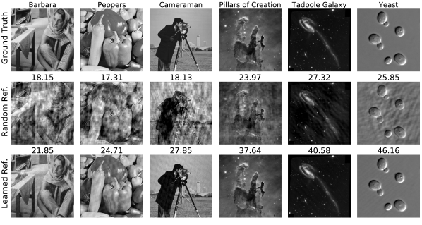
We present the results for these different datasets using references learned from 32 images from the same dataset in Fig. 2. We present results for six standard images of size $512\times 512$ from [34] using a resized reference learned from CelebA dataset in Fig. 3.

Measurements. We simulated amplitude measurements of the 2D Fourier transform. We performed 4 times oversampling in the spatial domain for both reference and target signal. Unless otherwise mentioned, we consider our measurements to be noise-free. We also report results for noisy measurements.

4.1 Configurations of Reference (u)

The reference signal $u$, which we are trying to learn, has a number of hyper-parameters that inherently affect the performance of the phase retrieval process. We considered several constraints on $u$, including the support, size, range, position, and sparsity.

We tested reference signals with both complex and real values and found that $u$ has comparable results in the two domains. Since it is easy to physically create amplitude or phase-only reference signals, we constrain $u$ to be in the real domain; thus, $u\in\mathbb{R}^{m\times n}$ and $m$, $n$ represent height and width, respectively. The height and width of $u$ determine the overlapping area between the target signal and the reference. We found that $u$ with larger size tends to have better performance, especially when the value of $u$ is constrained to a small range. The intensity values of $u$ play a major role in its performance. If we constrain the value of $u$ to be within a certain range: $u[i,j]\in[u_{min},u_{max}]$, for all $i,j$, we observed that bigger range of $u$ yields better performance. This is because when $u$ is unconstrained then we can construct a $u$ with a large norm. Consider the noiseless setting with quadratic measurements $|F(x+u)|^{2}=|Fx|^{2}+|Fu|^{2}+2\text{Re}(Fx\odot Fu)$, the last term is the real value of the element-wise product of target and reference Fourier transforms. We can remove $|Fu|^{2}$ because it is known. If $u$ is large compared to $x$, then we can also ignore the quadratic term $|Fx|^{2}$ and recover $x$ in a single iteration if all entries of $Fu$ are nonzero. To avoid this situation and make the problem stable in the presence of noise, we restricted the values in the reference $u$ to be in [0,1] range.

4.2 Setup of Training Samples and Sample Size

We observed that we can learn the reference signal from a small number of training images. In Table 1, we report test results for different reference signals learned on first $N$ images from MNIST training dataset for $N=32,128,512$. We kept the signal and reference strength (i.e., the range of the signal) equal for this experiment. We observe that increasing the training size improves test performance. However, we can get reasonable reconstruction performance on large test datasets (10k+ images) with reference learned using only 32 images.

Table 1: PSNR for different training sizes

Train/Test	MNIST	EMNIST	F. MNIST	SVHN	CIFAR10
Training size=32	66.54	58.72	57.81	57.51	41.60
Training size=128	76.25	64.16	55.86	59.50	44.34
Training size=512	79.14	62.34	52.01	59.78	48.90

4.3 Generalization of Reference on Different Classes

We are interested in evaluating the generalization of our learned reference. (i.e., how the reference performs when trained on one dataset and tested on another). In the comparison study, we took the reference $u$ trained on each dataset and then tested them on the remaining 4 datasets. The value range of the reference is between $[0,1]$, the number of steps in the unrolled network is $K=50$. We observed that when the datasets share great similarity (e.g., MNIST and EMNIST are both sparse digits or letters), the reference signal tends to work well on both datasets. Even when the datasets differ greatly in their distributions, the reference trained on one dataset provides good results on other datasets (with only a few dB of PSNR decrease in performance).

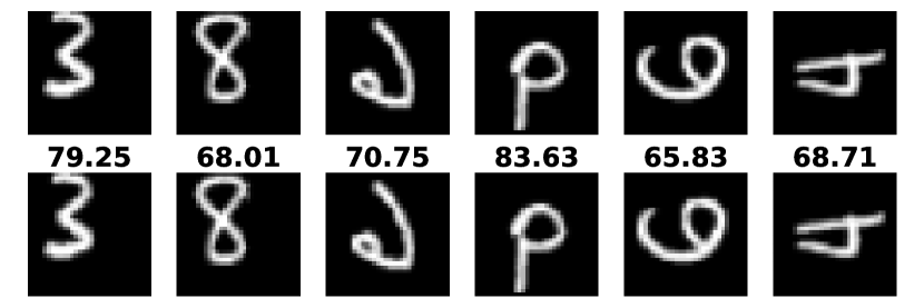
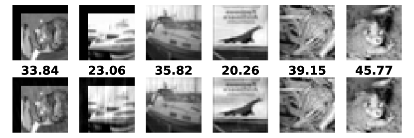
We also tested our method on shifted and rotated versions of test images. Results in Fig. 4 demonstrate that even though the reference was trained on upright and centered images, we can perfectly recover shifted and rotated images.

Our key insight about this generalization phenomenon is that the main challenge in Fourier phase retrieval methods is initialization and ambiguities that arise because of symmetries. We are able to solve these issues using a learned reference because of the following reasons: (1) A reference gives us a good initialization for the phase retrieval iterations. (2) The presence of a reference breaks the symmetries that arise in Fourier amplitude measurements. Moreover, we are not learning to solve the phase retrieval problem in an end-to-end manner or learn a signal-dependent denoiser to solve the inverse problem [34, 40]. We are learning reference signals to primarily help a predefined phase retrieval algorithm to recover the true signal from the phaseless measurements. Thus, the references learned on one class of images provide good results on other images, see Table 2. This study shows that the reference learned using our network has the ability to generalize to new datasets, thus making our method suitable for real-life applications where new test cases keep emerging.

(a) MNIST

(b) CIFAR10

Figure 4: Test results on shifted/flipped/rotated images using the reference learned on upright and centered (canonical) training images. (PSNR shown on top of images.)

Table 2: PSNR with references trained and tested on different datasets

Train/Test	MNIST	EMNIST	F. MNIST	SVHN	CIFAR10
MNIST	66.54	55.12	40.87	41.87	31.72
EMNIST	72.84	58.72	52.18	55.42	48.16
F. MNIST	40.87	55.67	57.81	50.70	42.85
SVHN	41.87	46.76	49.60	57.51	51.54
CIFAR10	31.72	38.93	36.40	40.36	41.60

4.4 Noise Response

To test the robustness of our method in the presence of noise, we added Gaussian and Poisson noise at different levels to the measurements. Poisson noise or shot noise is the most common in the practical systems. We model the Poisson noise following the same approach as in [34]. We simulate the measurements as

$$y(i)=|z(i)|+\eta(i)\;\;\;\text{for all }i=1,2,\ldots,m,$$ (12)

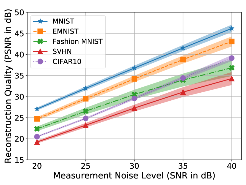
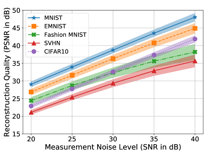
where $\eta(i)\sim\mathcal{N}(0,\sigma^{2})$ for Gaussian noise and $\eta(i)\sim\mathcal{N}(0,\lambda|z(i)|)$ for Poisson noise with $z=Ax+Bu$. We varied $\sigma,\lambda$ to generate noise at different signal-to-noise ratios. Poisson noise affects the larger measurements with higher strength than the smaller measurements. As the sensors can measure only positive measurements, we kept the measurements positive by applying ReLU function after noise addition. We can observe the effect of noise in Fig. 5. Even though we did not add noise during training, we get reasonable reconstruction and performance degrades gracefully with increased noise.

(a) Gaussian

(b) Poisson

Figure 5: Reconstruction quality of the test images vs noise level of the measurements for different datasets. We learned the reference using noise-free measurements.

4.5 Random Reference versus Learned Reference

To demonstrate the advantage of the learned reference signal, we compared the performance of learned reference and random reference on some standard images. The results are shown in Fig. 3. The learned reference is trained using 32 images from CelebA dataset which we resized to $200\times 200$. The test images used in Fig. 3 are $512\times 512$, so we resized the learned reference from $200\times 200$ to $512\times 512$. For random reference, we selected the entries of the reference uniformly at random from $[0,1]$. We selected the best result out of 100 trials for every test image with random reference. We can observe from the results that our learned reference significantly outperforms the random reference even though the test image distribution is distinct from the training data. The number of steps of the unrolled network is $K=50$.

4.6 Comparison with Existing Phase Retrieval Methods

We have shown comparison with other approaches in Table 3. We selected Kaczmarz [49] and Amplitude flow [11] for comparison using PhasePack package [9]. We also show Hybrid Input Output (HIO), which is similar to our phase retrieval routine without any reference. We observe that our approach with learned reference can outperform all other approaches on all the datasets. All the traditional phase retrieval methods suffer from the trivial circular shift, rotation, and flip ambiguities, thus produce significantly worse reconstruction than our method does. Our method uses a reference signal to simplify the initialization and removes the shift/reflect ambiguities. To mathematically explain this fact, a shifted or flipped version of $x$ would not give us the same Fourier measurements as $|F(x+u)|$ if $u$ is chosen appropriately as we do with the learning procedure. As we showed in Fig. 5, our method can perfectly recover the shifted and flipped versions of the images using the reference that was trained with upright and centered images.

Table 3: Comparison with existing phase retrieval methods

Methods	MNIST	EMNIST	F. MNIST	SVHN	CIFAR10
HIO	9.04	8.42	9.65	19.87	14.70
Amplitude Flow	9.99	9.79	11.90	20.25	15.04
Kaczmarz	11.81	11.47	13.44	19.48	15.01
Flat Reference	18.21	17.24	16.56	20.89	15.81
Random Reference	36.87	28.41	27.27	36.45	25.57
Learned Reference (Ours)	66.54	58.72	57.81	57.51	41.60

4.7 Effects of Number of Layers (K)

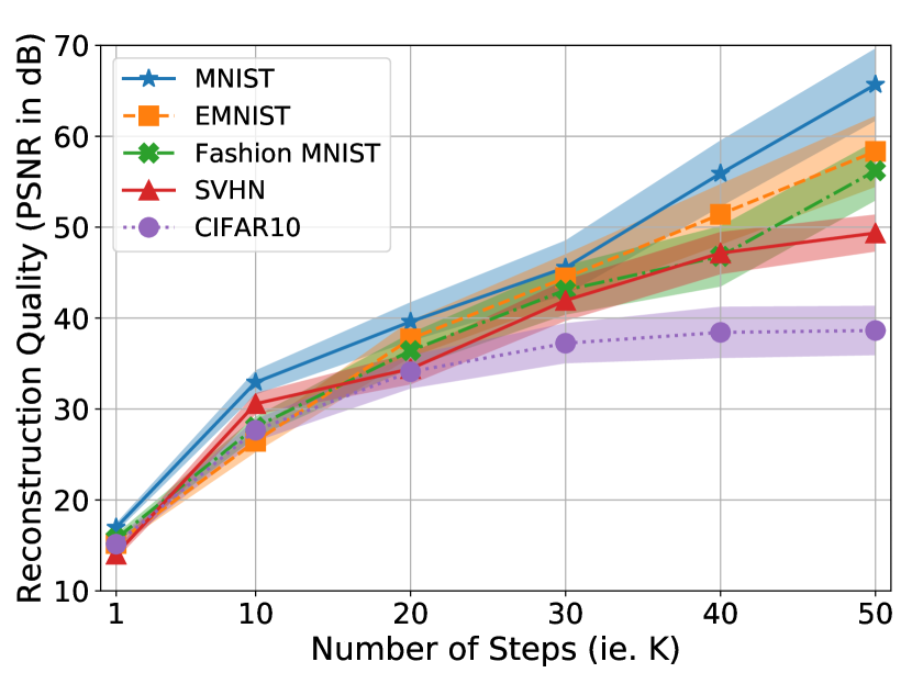
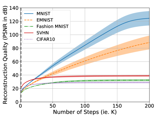
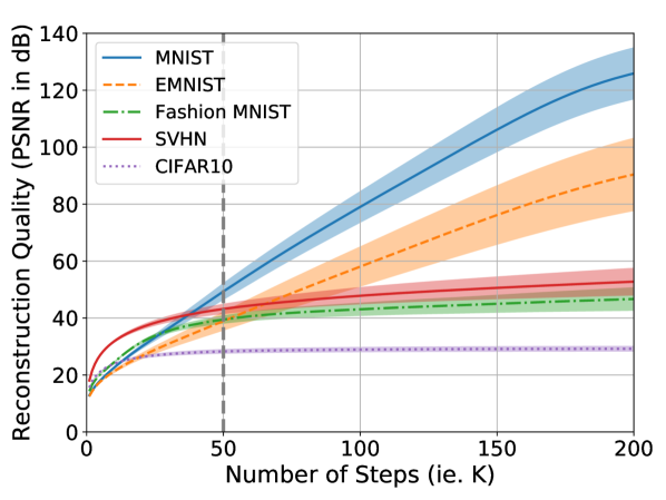
We tested our unrolled network with different numbers of layers (i.e., $K$) at training and test time. The results are summarized in Fig. 6. We first used the same values of $K$ for training and testing. We observed that as $K$ increases, the reconstruction quality (measured in PSNR) improves. Then we fixed $K=1$ or $K=50$ at training, but used different values of $K$ at testing. We observed that if we increase $K$ at the test time, PSNR improves up to a certain level and then it plateaus. The PSNR achieved with reference trained with $K=50$ is better than what the referenced trained with $K=1$ provided. These results provide us a trade-off between the reconstruction speed and quality. As we increase $K$, the reconstruction quality improves but the reconstruction requires more steps (computations and time).

Finally, we learned a reference using $K=1$ and tested it on different images with $K=1$. To our surprise, our method was able to produce reasonable quality reconstruction with this extreme setting. We present some single-step reconstructions of each data set in Fig. 7.

(a) Training K=Testing K

(b) Training K=1

(c) Training K=50

Figure 6: Reconstruction PSNR vs the number of blocks ($K$) in the unrolled network at training and testing. (a) $K$ is same for training and testing (shaded region shows $\pm 0.25$ times std of PSNR). (b) $K=1$ and (c) $K=50$, but tested using different $K$.

Figure 7: Single step reconstruction with reference in range $[0,1]$. Each of the 6 sets (a)-(f) has the the ground truth in the first row. Second row is the reconstruction (PSNR shown on top of images.)

4.8 Localizing the Reference

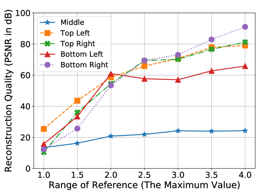
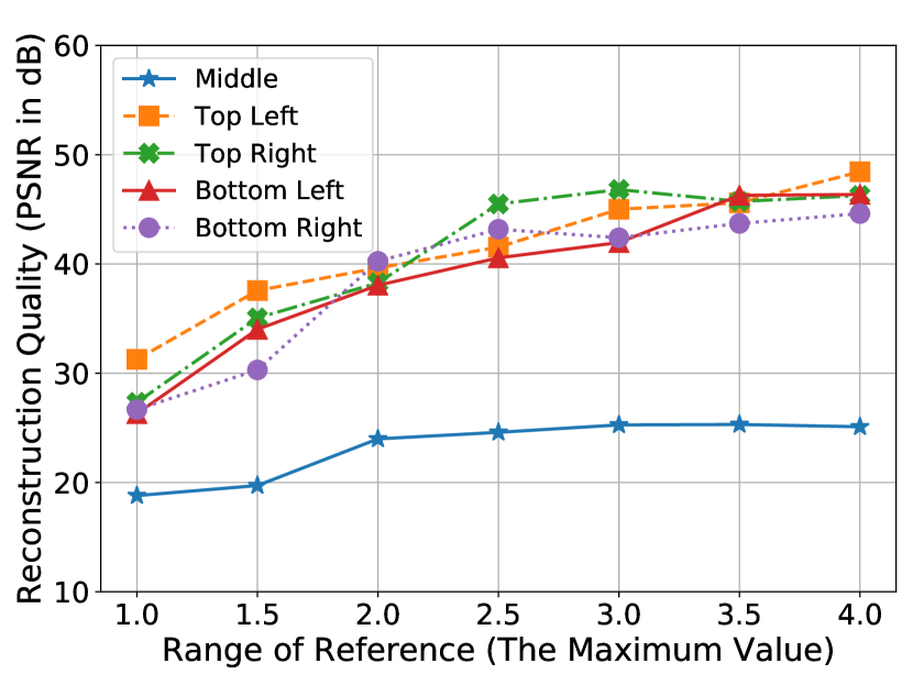
We also evaluated the effect of localizing the reference to a small region. For example, the reference is constrained to be within a small block in the corner or the center of the target signal. We restricted $u$ to be an $8\times 8$ block and placed it in different positions. We found that corner positions provide better results as shown in Fig. 8. As we bring the reference support closer to the center, the quality of reconstruction deteriorates. This observation is related to the method in [3, 18, 1], where if the known reference signal is separated from the target signal, then the phase retrieval problem can be solved as a linear inverse problem.

Note that signal recovery from Fourier phase retrieval is equivalent to signal recovery from its autocorrelation. We can write the autocorrelation of target plus reference signals as $(x+u)\star(x+u)=x\star x+u\star u+x\star u+u\star x$. The first term is a quadratic function of $x$, the second term is known, and the last two terms are linear functions of $x$. If the supports for $x$ and $u$ are sufficiently separated, then we can separate the last two linear terms from the first two quadratic terms and recover $x$ by solving a linear problem. However, if $x$ and $u$ have a significant overlap, then we need to solve a nonlinear inverse problem as we do in this paper.

(a) MNIST

(b) CIFAR10

Figure 8: Performance of our method if the reference is an $8\times 8$ block placed at different positions. Fixing the minimum value at 0, we increased the maximum value of the reference we learn. We observe that the small reference placed in the corners performs better than the ones placed in the center.

5 Conclusion

We presented a framework for learning a reference signal to solve the Fourier phase retrieval problem. The reference signal is learned using a small number of training images using an unrolled network as a solver for the phase retrieval problem. Once learned, the reference signal serves as a prior which significantly improves the efficiency of the signal reconstruction in the phase retrieval process. The learned reference generalizes to a broad class of datasets with different distribution compared to the training samples. We demonstrated the robustness and efficiency of our method through extensive experiments.

References

- [1] Arab, F., Asif, M.S.: Fourier phase retrieval with arbitrary reference signal. In: ICASSP 2020-2020 IEEE International Conference on Acoustics, Speech and Signal Processing (ICASSP). pp. 1479–1483. IEEE (2020)
- [2] Bahmani, S., Romberg, J.: Efficient compressive phase retrieval with constrained sensing vectors. In: Proc. Adv. in Neural Inf. Proc. Sys. (NeurIPS). pp. 523–531 (2015)
- [3] Barmherzig, D., Sun, J., Li, P., Lane, T., Candès, E.: Holographic phase retrieval and reference design. Inverse Problems (2019)
- [4] Bostan, E., Kamilov, U.S., Waller, L.: Learning-based image reconstruction via parallel proximal algorithm. IEEE Signal Processing Letters 25(7), 989–993 (2018)
- [5] Cai, T., Li, X., Ma, Z., et al.: Optimal rates of convergence for noisy sparse phase retrieval via thresholded wirtinger flow. Ann. Stat. 44(5), 2221–2251 (2016)
- [6] Candes, E., Li, X., Soltanolkotabi, M.: Phase retrieval from coded diffraction patterns. Appl. Comput. Harmon. Anal. 39(2), 277–299 (2015)
- [7] Candes, E., Li, X., Soltanolkotabi, M.: Phase retrieval via wirtinger flow: theory and algorithms. IEEE Trans. Inform. Theory 61(4), 1985–2007 (2015)
- [8] Candes, E., Strohmer, T., Voroninski, V.: Phaselift: Exact and stable signal recovery from magnitude measurements via convex programming. Comm. Pure Appl. Math. 66(8), 1241–1274 (2013)
- [9] Chandra, R., Zhong, Z., Hontz, J., McCulloch, V., Studer, C., Goldstein, T.: Phasepack: A phase retrieval library. Asilomar Conference on Signals, Systems, and Computers (2017)
- [10] Chang, H., Lou, Y., Ng, M., Zeng, T.: Phase retrieval from incomplete magnitude information via total variation regularization. SIAM Journal on Scientific Computing 38(6), A3672–A3695 (2016)
- [11] Chen, Y., Candes, E.: Solving random quadratic systems of equations is nearly as easy as solving linear systems. In: Proc. Adv. in Neural Inf. Proc. Sys. (NeurIPS). pp. 739–747 (2015)
- [12] Chen, Z., Jagatap, G., Nayer, S., Hegde, C., Vaswani, N.: Low rank fourier ptychography. In: 2018 IEEE International Conference on Acoustics, Speech and Signal Processing (ICASSP). pp. 6538–6542 (April 2018)
- [13] Diamond, S., Sitzmann, V., Heide, F., Wetzstein, G.: Unrolled optimization with deep priors. arXiv preprint arXiv:1705.08041 (2017)
- [14] Fienup, J.R.: Phase retrieval algorithms: a comparison. Applied optics 21(15), 2758–2769 (1982)
- [15] Gerchberg, R.W.: A practical algorithm for the determination of phase from image and diffraction plane pictures. Optik 35, 237–246 (1972)
- [16] Gregor, K., LeCun, Y.: Learning fast approximations of sparse coding. In: Proceedings of the 27th International Conference on International Conference on Machine Learning. pp. 399–406 (2010)
- [17] Gross, D., Krahmer, F., Kueng, R.: Improved recovery guarantees for phase retrieval from coded diffraction patterns. Appl. Comput. Harmon. Anal. 42(1), 37–64 (2017)
- [18] Guizar-Sicairos, M., Fienup, J.: Holography with extended reference by autocorrelation linear differential operation. Optics express 15(26), 17592–17612 (2007)
- [19] Hammernik, K., Klatzer, T., Kobler, E., Recht, M.P., Sodickson, D.K., Pock, T., Knoll, F.: Learning a variational network for reconstruction of accelerated mri data. Magnetic resonance in medicine 79(6), 3055–3071 (2018)
- [20] Hand, P., Leong, O., Voroninski, V.: Phase retrieval under a generative prior. In: Proc. Adv. in Neural Inf. Proc. Sys. (NeurIPS). pp. 9154–9164 (2018)
- [21] Harrison, R.: Phase problem in crystallography. JOSA a 10(5), 1046–1055 (1993)
- [22] Hyder, R., Hegde, C., Asif, M.: Fourier phase retrieval with side information using generative prior. In: Proc. Asilomar Conf. Signals, Systems, and Computers. IEEE (2019)
- [23] Hyder, R., S., V., Hegde, C., Asif, M.: Alternating phase projected gradient descent with generative priors for solving compressive phase retrieval. In: Proc. IEEE Int. Conf. Acoust., Speech, and Signal Processing (ICASSP). pp. 7705–7709. IEEE (2019)
- [24] Jaganathan, K., Oymak, S., Hassibi, B.: Recovery of sparse 1-d signals from the magnitudes of their fourier transform. In: Proc. IEEE Int. Symp. Inform. Theory (ISIT). pp. 1473–1477. IEEE (2012)
- [25] Jagatap, G., Chen, Z., Hegde, C., Vaswani, N.: Sub-diffraction imaging using fourier ptychography and structured sparsity. In: 2018 IEEE International Conference on Acoustics, Speech and Signal Processing (ICASSP). pp. 6493–6497 (April 2018)
- [26] Jagatap, G., Chen, Z., Nayer, S., Hegde, C., Vaswani, N.: Sample efficient fourier ptychography for structured data. IEEE Transactions on Computational Imaging 6, 344–357 (2020)
- [27] Jagatap, G., Hegde, C.: Fast, sample-efficient algorithms for structured phase retrieval. In: Advances in Neural Information Processing Systems. pp. 4917–4927 (2017)
- [28] Jagatap, G., Hegde, C.: Algorithmic guarantees for inverse imaging with untrained network priors. In: Advances in Neural Information Processing Systems. pp. 14832–14842 (2019)
- [29] Kamilov, U.S., Mansour, H.: Learning optimal nonlinearities for iterative thresholding algorithms. IEEE Signal Processing Letters 23(5), 747–751 (2016)
- [30] Kellman, M., Bostan, E., Chen, M., Waller, L.: Data-driven design for fourier ptychographic microscopy. International Conference for Computational Photography pp. 1–8 (2019)
- [31] Kellman, M.R., Bostan, E., Repina, N.A., Waller, L.: Physics-based learned design: optimized coded-illumination for quantitative phase imaging. IEEE Transactions on Computational Imaging 5(3), 344–353 (2019)
- [32] Li, X., Voroninski, V.: Sparse signal recovery from quadratic measurements via convex programming. SIAM J. on Math. Analysis 45(5), 3019–3033 (2013)
- [33] Maiden, A., Rodenburg, J.: An improved ptychographical phase retrieval algorithm for diffractive imaging. Ultramicroscopy 109(10), 1256–1262 (2009)
- [34] Metzler, C.A., Schniter, P., Veeraraghavan, A., Baraniuk, R.G.: prdeep: Robust phase retrieval with a flexible deep network. In: Proc. Int. Conf. Machine Learning (2018)
- [35] Millane, R.: Phase retrieval in crystallography and optics. JOSA A 7(3), 394–411 (1990)
- [36] Netrapalli, P., Jain, P., Sanghavi, S.: Phase retrieval using alternating minimization. In: Proc. Adv. in Neural Inf. Proc. Sys. (NeurIPS). pp. 2796–2804 (2013)
- [37] Nolte, D.D.: Optical interferometry for biology and medicine, vol. 1. Springer Science & Business Media (2011)
- [38] Ohlsson, H., Yang, A., Dong, R., Sastry, S.: Cprl–an extension of compressive sensing to the phase retrieval problem. In: Proc. Adv. in Neural Inf. Proc. Sys. (NeurIPS). pp. 1367–1375 (2012)
- [39] Park, I., Middleton, R., Coggrave, C.R., Ruiz, P.D., Coupland, J.M.: Characterization of the reference wave in a compact digital holographic camera. Applied optics 57(1), A235–A241 (2018)
- [40] Rivenson, Y., Zhang, Y., Günaydın, H., Teng, D., Ozcan, A.: Phase recovery and holographic image reconstruction using deep learning in neural networks. Light: Science & Applications 7(2), 17141–17141 (2018)
- [41] Rodenburg, J.M.: Ptychography and related diffractive imaging methods. Advances in imaging and electron physics 150, 87–184 (2008)
- [42] Shamshad, F., Ahmed, A.: Robust compressive phase retrieval via deep generative priors. arXiv preprint arXiv:1808.05854 (2018)
- [43] Shechtman, Y., Eldar, Y., Cohen, O., Chapman, H., Miao, J., Segev, M.: Phase retrieval with application to optical imaging: a contemporary overview. IEEE Signal Processing Mag. 32(3), 87–109 (2015)
- [44] Tahara, T., Quan, X., Otani, R., Takaki, Y., Matoba, O.: Digital holography and its multidimensional imaging applications: a review. Microscopy 67(2), 55–67 (2018)
- [45] Wang, G., Giannakis, G.: Solving random systems of quadratic equations via truncated generalized gradient flow. In: Proc. Adv. in Neural Inf. Proc. Sys. (NeurIPS). pp. 568–576 (2016)
- [46] Wang, G., Zhang, L., Giannakis, G.B., Akcakaya, M., Chen, J.: Sparse phase retrieval via truncated amplitude flow. IEEE Trans. Signal Processing 66, 479–491 (2018)
- [47] Wang, G., Giannakis, G., Saad, Y., Chen, J.: Solving most systems of random quadratic equations. In: Advances in Neural Information Processing Systems. pp. 1867–1877 (2017)
- [48] Wang, S., Fidler, S., Urtasun, R.: Proximal deep structured models. In: Advances in Neural Information Processing Systems. pp. 865–873 (2016)
- [49] Wei, K.: Solving systems of phaseless equations via kaczmarz methods: A proof of concept study. Inverse Problems 31(12), 125008 (2015)
- [50] Yang, Y., Sun, J., Li, H., Xu, Z.: Deep admm-net for compressive sensing mri. In: Advances in neural information processing systems. pp. 10–18 (2016)
- [51] Yuan, Z., Wang, H.: Phase retrieval with background information. Inverse Problems 35(5), 054003 (may 2019)
- [52] Zhang, H., Liang, Y.: Reshaped wirtinger flow for solving quadratic system of equations. In: Proc. Adv. in Neural Inf. Proc. Sys. (NeurIPS). pp. 2622–2630 (2016)