Magnetic fields in late-stage proto-neutron stars

Abstract

We explore the thermal and magnetic-field structure of a late-stage proto-neutron star. We find the dominant contribution to the entropy in different regions of the star, from which we build a simplified equation of state for the hot neutron star. With this, we numerically solve the stellar equilibrium equations to find a range of models, including magnetic fields and rotation up to Keplerian velocity. We approximate the equation of state as a barotrope, and discuss the validity of this assumption. For fixed magnetic-field strength, the induced ellipticity increases with temperature; we give quantitative formulae for this. The Keplerian velocity is considerably lower for hotter stars, which may set a de-facto maximum rotation rate for non-recycled NSs well below 1 kHz. Magnetic fields stronger than around $10^{14}$ G have qualitatively similar equilibrium states in both hot and cold neutron stars, with large-scale simple structure and the poloidal field component dominating over the toroidal one; we argue this result may be universal. We show that truncating magnetic-field solutions at low multipoles leads to serious inaccuracies, especially for models with rapid rotation or a strong toroidal-field component.

1 Introduction

In the first phase of its life, a highly-magnetised neutron star (NS) has the potential to radiate a huge amount of energy, through both electromagnetic and gravitational waves. These signals are of great interest, containing information that could allow us to constrain processes involving elementary constituents of matter under extreme astrophysical conditions, the nuclear physics of hot dense matter, the fluid dynamics of the newborn star, and the dynamo processes driving magnetic-field amplification in extremely highly-conducting media.

With their astrophysical importance and complexity, supernovae and proto-neutron stars have long been studied through numerical evolutions (see e.g. Colgate & White (1966); Burrows & Lattimer (1986); Janka et al. (2007)), and their hydrodynamics and microphysics – among other aspects – remain topics of active study. By contrast, the magnetic field of the newborn NS has received relatively little attention, especially given that this phase is likely to be the most dramatic of the field’s life. It is likely that some remnant field of the progenitor star is amplified and rearranged during this phase (Thompson & Duncan, 1993), but we lack any quantitative understanding of this process.

For a cooling, mature NS we have a better – though still incomplete – understanding of its magnetic field. In particular, a reasonably complete picture of magnetic-field evolution within the star’s solid crust has emerged after sustained attention; see Pons & Viganò (2019) for a recent review. Core evolution is far less certain, though may be too slow to be of relevance to many problems. Complementary to these evolutions are a number of studies of possible equilibrium states of a magnetised NS, solving for the global field but without accounting for the evolutionary history frozen into the crust; for a brief but representative selection of these models see, e.g., Bocquet et al. (1995); Kiuchi et al. (2009); Ciolfi et al. (2010); Lander (2014); Glampedakis et al. (2014); Pili et al. (2015).

In comparison with the attention shown to the star’s birth and maturity, the late proto-NS phase (covering a period from some ten seconds to roughly a few minutes after birth) is terra incognita, especially for the star’s magnetic field. It may, however, be a very important stage in the star’s evolution: one where the physics driving the star’s birth phase will have ceased, but thermal effects will still be important. Magnetic-field rearrangement during this early era, rather than any dynamo mechanism, may be what sets the basic long-term structure of the mature star’s field. The resultant field configurations would also be the logical initial condition for field-evolution studies. In this paper we aim to explore the late proto-NS phase in more detail, looking at the main contributions to the star’s thermal structure and finding equilibrium states for a magnetised NS at high temperature.

1.1 Supernova and aftermath

The life of a massive star culminates in the gravitational collapse of its core. If the star’s mass is more than a few tens of times that of the Sun, the collapse continues unabated until a black hole is formed. Otherwise, the compression of matter is brought to a halt by the high stiffness (incompressibility) of uniform nuclear matter, causing a bounce. This occurs on a surface enclosing the denser half of the mass of the future proto NS and sends a shock wave through the envelope, heating it strongly and lifting infalling stellar matter, and thus separating a hot and dense central object from the pre-supernova star doomed to explosion (Woosley et al., 2002). A proto NS is born. Its initial internal temperature, $T$, and entropy per baryon, $s_{b}$, are very non-uniform, with maxima reached in the shocked half of the mass.

Initially, a proto NS is opaque to neutrinos, and the total electron lepton number per baryon $Y_{L_{\textrm{e}}}$ (a sum of electron $Y_{\textrm{e}}$ and electron neutrino $Y_{\nu_{\textrm{e}}}$ contributions) is $\approx 0.35$, only slightly smaller than in the presupernova iron-nickel core. During the next seconds the proto-NS deleptonizes via $\nu_{\textrm{e}}$ diffusion driven by the $Y_{\nu_{\textrm{e}}}$ gradient. The $\nu_{\textrm{e}}$ thermalize, losing their degeneracy, and leave the star through the neutrinosphere (the surface at which matter becomes neutrino-transparent). The transport of lepton number and energy by diffusion is accelerated by convective flows. Diffusion of $\nu_{\textrm{e}}$ outwards is associated with heating of the matter by the $\nu_{\textrm{e}}$ downscattering. After $\sim 10$ s deleptonization has been completed, gradients of $T$ and $s_{b}$ smoothed, and convective stability reached. Neutrino-antineutrino pairs of all three flavours still transport heat via diffusion towards the neutrinosphere, and are radiated there (Prakash et al., 1997). The proto NS enters its late stage, the subject of the present study.

During the next minute or so, with a composition not very different from that of a mature NS, the proto NS is still hot, $\sim 5\times 10^{10}~{}$K in the core, with an envelope composed of a plasma of nuclei, neutrons, and electrons, and density above $10^{11}~{}{\rm g~{}cm^{-3}}$. The envelope is neutrino-opaque, and layers above it contain the flavour-dependent, rather thick, neutrinospheres. The envelope is liquid, even in its deepest layers close to the core. Its temperature is decreasing outwards. As we assume slow neutrino cooling (no direct Urca in the core), at this late proto NS stage both $T$ and $s_{b}$ are slowly varying within the core, decreasing more rapidly towards the neutrinospheres. In the present paper we assume that there is no plasma fallback after a successful shock take-off.

The pressure in a mature NS core is due to nuclear forces and to a lesser extent, to the degeneracy of the neutrons (Cameron, 1959). In the inner envelope, where nuclei are immersed in a neutron gas, the pressure is supplied by the degeneracy of the neutron gas, with the contribution from nuclear forces in dripped neutron gas rapidly increasing close to the core. This is in contrast to normal, non-degenerate stars, where pressure is thermal in nature; these stars are hot, powered by fusion processes. The proto-NS phase has the distinguishing feature that both neutron-degeneracy and thermal pressure play a role in determining the stellar structure; with neutrinos flooding out of the newborn star once it becomes neutrino-transparent, this phase is over within a few minutes (Burrows & Lattimer, 1986; Pons et al., 1999). However, this brief period of time – which has not been previously explored in the context of magnetic-field modelling – is a crucial one to understand. It constitutes a missing link between work on the dynamic evolution and generation of magnetic fields in proto-NSs, as described next, and the far slower, secular evolution in mature neutron stars.

The minute following a NS’s birth is crucial for the star’s magnetic field. The magnetic field of the progenitor star’s degenerate core will be amplified by compression to nuclear densities during stellar core collapse, but this alone is unlikely to explain the field strengths of NSs, especially magnetars, where the external field is around $10^{15}$ G and the internal field perhaps an order of magnitude stronger. Instead, dynamo processes act to amplify and rearrange the field; these could involve some combination of differential rotation, convection and the magneto-rotational instability (for a review of this topic, see Spruit (2009)). These processes are likely to cease at a very early phase, with the dynamo saturating and becoming inhibited, magnetic coupling flattening the rotation profile so the star’s rotation becomes uniform, and turbulent convection ceasing as the stellar matter becomes neutrino-transparent.

1.2 The early quasi-equilibrium

Whatever magnetic field has been created in the birth phase will afterwards start to rearrange, in an attempt to attain an approximate equilibrium with the fluid star. It is perhaps possible that it fails to settle in this way and instead reaches some kind of ‘average’ steady state, where the star still exhibits short-term dynamics but average values of energy quantities are roughly constant (Sur et al., 2020), though it is likely that over longer timescales this would dissipate considerable amounts of energy. Here we will assume that the magnetised star does indeed reach a true equilibrium – one that is also dynamically stable, and so a natural endpoint for the rearrangement.

To establish when the star can be treated as in approximate equilibrium, we first need to know how quickly the magnetic field can adapt to its host fluid. Assuming, for the time being, a non-rotating star, the field is able to rearrange locally over the time $\tau_{A}$ taken for an Alfvén wave to cross the region concerned. Defining $l_{B}$ as the distance crossed and $v_{A}$ as the Alfvén speed, we have

$$\tau_{A}\sim\frac{l_{B}}{v_{A}}\sim \frac{l_{B}\sqrt{4\pi\rho}}{B}$$

$$\approx 1.1\left({\frac{B}{10^{14}\textrm{ G}}}\right)^{-1}\left({\frac{\rho}{10^{15}\textrm{ g cm}^{-3}}}\right)^{1/2}\left({\frac{l_{B}}{10\textrm{ km}}}\right)\textrm{ s}$$ (1)

where $B$ is the magnetic field strength, $\rho$ the rest-mass density, and where we have normalised $l_{B}$ to 10 km to get a timescale for global magnetic-field rearrangement. Implicit in the above estimate is that the star is entirely fluid; we confirm this in section 2.2.2, with quantitative calculations of the state of matter of the proto-NS.

Note that this estimate may not be reliable for the very rapidly rotating models we consider later in this paper; it is known, for example, that in the presence of rotation Alfvén oscillation modes are replaced by magneto-inertial modes (see, e.g., Lin & Ogilvie (2018) and references therein). These modes tend to be of higher frequency than their non-rotating counterparts (Lander et al., 2010; Lander & Jones, 2011), leading to a shorter $\tau_{A}$ and thus suggesting that the magnetic field may be able to re-equilibrate to the fluid more quickly at increasing rotation rate. The opposite conclusion was, however, reached by Braithwaite & Cantiello (2013) from timescale arguments, although these authors made the simplication of not explicitly considering the centrifugal distortion to the star. Fortunately this uncertainty does not have any serious impact on our main results.

Now, if the Alfvén timescale $\tau_{A}$ is short compared with the cooling timescale of the star, the magnetic field should always have time to readjust to the new thermal state of the star, and therefore may be thought of as proceeding through a sequence of quasi-equilibria. In this case, an individual equilibrium model may be thought of as a snapshot of this process. We defer the more technical discussion of the role of chemical equilibrium to section 3.2.

We can make a rough estimate of the cooling timescale for a proto-NS from visual inspection of the plots of Burrows & Lattimer (1986) or similar work; it is of order $10$ s. Therefore, for large-scale magnetic fields stronger than roughly $10^{14}$ G, the equilibrium approximation is reasonable even during this early phase. For weaker magnetic fields, it is possible that the field will spend this phase out-of-equilibrium with the fluid, retaining vestiges of the (presumably) complex magnetic-field structure produced by the birth. However, it is quite plausible that $10^{14}$ G does represent a typical birth magnetic-field strength, with the typical surface field strength decaying to pulsar-type values by the time we observe them. In any case, we consider here that class of late proto-NSs for whom a quasi-equilibrium approximation is reasonable.

1.3 Plan of the paper

This paper is arranged as follows. In section 2 we begin with a description of the equation of state and thermal physics of a hot neutron star, and describe more precisely the meaning of the ‘late’ proto-neutron star phase. We devise a simplified model of the thermal physics of the star, retaining the leading-order contributions in each region. In section 3 we discuss the general equilibrium equations and the equation of state, in particular the possible presence of buoyancy forces, and in section 4 we describe our prescription for the thermal pressure. Section 5 formulates the problem in a way we can solve numerically, and we give details of this solution method. Our results are presented in section 6, and we discuss their implications in section 7.

2 Thermal structure of a late proto-neutron star

2.1 Equation of state of a late proto-neutron star

2.1.1 Equation of state of the core

The core consists of a uniform plasma of mainly neutrons, with a small admixture of protons, electrons and muons. Thermodynamical quantities, such as internal energy per unit volume $U$, pressure $P$,…. are split into a $T=0$ (cold) part, $U_{0}$, $P_{0}$,…and a thermal contribution depending on $T$ and vanishing in the $T=0$ limit, e.g., $U_{\rm th},P_{\rm th},\ldots$. For the $T=0$ equation of state (EOS) we choose an approximation of the SLy EOS (Douchin & Haensel, 2001) by a piecewise polytrope. Then we get the $T=0$ values of the baryon chemical potential from $\mu_{0}=m_{\rm u}c^{2}+(U_{0}+P_{0})/n$ and the matter density, including rest energy of nucleons, $\rho_{0}=m_{\rm u}n+U_{0}/c^{2}$, where $n$ is the baryon number density, and $m_{\rm u}$ is the atomic mass unit. The thermal components of the core EOS are approximated by those of an ideal, nonrelativistic, strongly degenerate Fermi gas of neutrons, with number density $n$. The Fermi momentum and Fermi energy of a degenerate gas of free neutrons, $p_{\rm Fn}$, are related to $n$ by $p_{\rm Fn}=\hbar(3\pi^{2}n)^{1/3}$, $\varepsilon_{\rm Fn}=\hbar^{2}(3\pi^{2}n)^{2/3}/(2m_{\rm u})$. Because of the supranuclear densities prevailing in the core, it is convenient to express $n$ in the units of normal nuclear density $n_{0}=0.16~{}{\rm fm^{-3}}$. We therefore define $\overline{n}=n/n_{0}$. The core edge is at about $\overline{n}=0.5$. The Fermi energy and Fermi temperature of neutrons are in our approximation

$$\varepsilon_{{\rm Fn}}=58.44~{}{\overline{n}}^{2/3}~{}{\rm MeV}~{},~{}~{}T_{\rm F}=\varepsilon_{{\rm Fn}}/k_{\rm B}~{},$$ (2)

(3)

$$~{}~{}T/T_{{\rm Fn}}=1.47\times 10^{-2}~{}T_{10}/\overline{n}^{2/3}~{},$$ (4)

where $T_{10}=T/10^{10}~{}{\rm K}$. To find the thermal contributions to $U$,$P$, entropy density $S$, and neutron chemical potential $\mu$, we take those derived for a degenerate free nonrelativistic electron gas (§58 of Landau & Lifshitz (1993)) and replace the electron mass by the neutron one. Then, neglecting powers of $T/T_{{\rm Fn}}$ higher than two, we get:

$$U_{\rm th}={1\over 4}\pi^{2}n\varepsilon_{\rm Fn}(T/T_{\rm Fn})^{2}~{},~{}~{}P_{\rm th}={1\over 6}\pi^{2}n\varepsilon_{\rm Fn}(T/T_{\rm Fn})^{2}~{},$$ (5)

(6)

$$S_{\rm th}=S={1\over 2}\pi^{2}nk_{\rm B}{T/T_{\rm Fn}}~{},~{}~{}\mu_{\rm th}=-{1\over 12}\pi^{2}\varepsilon_{\rm Fn}(T/T_{\rm Fn})^{2}~{}.$$ (7)

Note that $S_{0}=0$ and $\mu_{0}=\varepsilon_{{\rm Fn}}$.

2.1.2 Equation of state and composition of the envelope

At $T=0$ the envelope is a solid crust of nuclei localized in the crystal lattice sites. Under the conditions prevailing in the late stage of a proto-NS, this ‘crust’ will in fact be a liquid envelope. In contrast to the core, the envelope is a nonuniform form of dense matter. It consists of nuclei, which for densities larger than the neutron drip density, $n_{\rm nd}$, (i.e., in the inner envelope) are immersed in a gas of unbound neutrons. At a given baryon density $n$ the envelope is treated as a plasma of one type of ions (nuclei), possibly immersed in an neutron gas, all permeated by a quasi-uniform electron gas. Within the envelope, we will use an approximate relation between $n$ and the matter density $\rho\simeq nm_{\rm u}$. We will use the SLy model of the $T=0$ crust (Douchin & Haensel, 2001), for consistency with our core prescription. As in the case of the uniform liquid core, the EOS of the envelope is split into a $T=0$ (cold) part, $U_{0}(\rho),P_{0}(\rho)$ and a thermal one, $U_{\rm th}(\rho,T),P_{\rm th}(\rho,T)$ vanishing in the limit of $T=0$. We introduce a set of parameters characterizing locally this layer of a late-stage proto-NS. These parameters are functions of the density $\rho$. The number density of ions (nuclei) is $n_{\rm i}$. The number of nucleons and number of protons in an ion are $A$ and $Z$, respectively. We define an ion sphere of radius $a_{\rm i}$ such that its volume $\frac{4}{3}\pi a_{\rm i}^{3}$ is equal to the volume per ion $1/n_{\rm i}$. The ion sphere contains a single ion at its centre and $Z$ electrons that neutralize the ion charge $Ze$. In the inner envelope a fraction of neutrons is unbound, and therefore the number of nucleons in an ion sphere is $A^{\prime}>A$. One must therefore specify the fraction of unbound neutrons in the total number of nucleons, $X_{\rm n}$. In the outer envelope $X_{\rm n}=0$. The fraction of volume occupied by nuclei will be denoted by $u$.

In what follows we derive the thermal part of the EOS of the envelope, to be added to the dominant $T=0$ part. Our notation follows Ch.2,3 of Haensel et al. (2007). We consider ions, unbound neutrons, electrons and their contributions to the thermodynamic quantities in the $T-\rho$ plane. We do not include thermal effects on the composition, which for our range of $T$ is reasonable for ${\rm log}(\rho/{\rm g~{}cm^{-3}})>10$.

We start with the simplest component of the envelope: the electrons. Already for ${\rm log}(\rho/{\rm g~{}cm^{-3}})>8$ electrons form a (nearly) uniform ultrarelativistic quasifree Fermi gas with Fermi energy

$$\varepsilon_{{\rm Fe}}=p_{{\rm Fe}}c=33.14~{}(n_{\textrm{e}}/10^{-3}n_{0})^{1/3}~{}{\rm MeV}~{}.$$ (8)

At neutron drip $\overline{n}=\overline{n}_{\rm nd}\approx 10^{-3}$ and $n_{\textrm{e}}\approx 0.3n_{\rm nd}$ so that $\varepsilon_{{\rm Fe}}^{\rm nd}\approx 22~{}{\rm MeV}$.

In our case, with ${\rm log}(\rho/{\rm g~{}cm^{-3}})>10$, the electrons are strongly degenerate, $T\ll T_{{\rm Fe}}=\varepsilon_{{\rm Fe}}/k_{\rm B}$. Keeping only the leading terms of an expansion in $T/T_{{\rm Fe}}$, we get the following formulae for the thermal contribution of the electrons (see §61 of Landau & Lifshitz (1993)):

$$U_{\rm th}={1\over 2}\pi^{2}n_{\textrm{e}}\varepsilon_{\rm F}\left({T/T_{{\rm Fe}}}\right)^{2}~{},~{}~{}~{}P_{\rm th}={1\over 6}\pi^{2}n_{\textrm{e}}\varepsilon_{{\rm Fe}}\left({T/T_{{\rm Fe}}}\right)^{2}~{},$$ (9)

(10)

$$S_{\textrm{e}}=\pi^{2}n_{\textrm{e}}k_{\rm B}~{}{T/T_{{\rm Fe}}}~{},~{}~{}~{}\mu_{\rm th}=-{1\over 3}\pi^{2}\varepsilon_{{\rm Fe}}\left({T/T_{{\rm Fe}}}\right)^{2}~{},$$ (11)

(12)

$$~{}~{}T_{{\rm Fe}}=38.46\times 10^{10}(n_{\textrm{e}}/10^{-3}n_{0})^{1/3}~{}{\rm K}~{}.$$ (13)

Next we turn to the ion component of the envelope, for which we need to define and calculate various parameters. Firstly, the number density of ions is expressed as $n_{\rm i}=\rho/(A^{\prime}m_{\rm u})$, and average charge neutrality implies $n_{\textrm{e}}=n_{\rm i}Z$. From these, we can now express the ion sphere radius $a_{\rm i}$ to plasma parameters in two ways:

$${4\over 3}\pi a_{\rm i}^{3}n=n_{\rm i}A^{\prime}/n=n_{\rm i}Z/n_{\rm e}~{}~{}.$$ (14)

We can understand the state of matter in the envelope through the dimensionless Coulomb coupling parameter for ions, which measures the relative strength of the Coulomb interaction of ions compared to the energy of their thermal motion:

$$\Gamma_{\rm i}={Z^{2}e^{2}\over a_{\rm i}k_{\rm B}T}~{}.$$ (15)

The strength of correlations between ions in the envelope and their contribution to the ion thermodynamical quantities can be expressed in terms of $\Gamma_{\rm i}$. The numerical value of $\Gamma_{\rm i}$ for a plasma can be readily obtained by passing to dimensionless variables:

$$\Gamma_{\rm i}={7.42\over T_{9}}\left({\rho_{10}\over A^{\prime}/100}\right)^{1/3}\left({Z\over 40}\right)^{2}~{},$$ (16)

where $\rho_{10}=\rho/10^{10}\;{\rm g~{}cm^{-3}}$ and $T_{9}=T/10^{9}\;{\rm K}$.

Using $\Gamma_{\rm i}$, we distinguish three main physical regimes of the plasma in the density-temperature plane. If $\Gamma_{\rm i}\ll 1$ then Coulomb correlations between ions are unimportant, and the thermal state of ions is well approximated by a Boltzmann gas model. Coulomb correlations become important when $\Gamma_{\rm i}\simeq 1$, and grow stronger and stronger with increasing $\Gamma_{\rm i}$. For a given $\rho$, $\Gamma_{\rm i}=1$ is reached at a characteristic temperature $T_{l}$ that may be found by rearranging Eq. (16):

$$T_{l}=9.504\times 10^{10}\left({Z\over 30}\right)^{2}\left({\rho_{10}\over{A^{\prime}/100}}\right)^{1/3}~{}{\rm K}~{}.$$ (17)

So at a given $\rho$, the ions behave as a nearly-ideal Boltzmann gas of nuclei if $T\gg T_{l}$. Then for smaller values of $T$ within $T_{m}<T\;\raise 1.29167pt\hbox{$<$\kern-7.5pt\raise-4.73611pt\hbox{$\sim$}}\;T_{l}$ (where $T_{m}$ is the melting temperature of an ion crystal) correlations are important and we are dealing with a strongly-coupled Coulomb liquid of ions. Finally, at an even lower $T=T_{m}$ the Coulomb liquid of ions crystallizes (solidifies) via a first order phase transition, with very small latent heat. Numerical simulations predict that to a very good approximation the free energy of the ion liquid (with quantum contributions negligible) is a function of $\Gamma_{\rm i}$ only. Crystallization occurs at $\Gamma_{\rm i}=175$ (Potekhin & Chabrier, 2000), which leads to (again using Eq. (16)):

$$T_{m}=5.43\times 10^{8}\left({Z\over 30}\right)^{2}\left({\rho_{10}\over{A^{\prime}/100}}\right)^{1/3}~{}{\rm K}~{}.$$ (18)

There is an additional plasma parameter that allows one to determine the relative importance of quantum effects in the thermal properties of the ion liquid. This is the plasma frequency for the ions $\omega_{\rm pi}$, corresponding to the frequency of vibrations generated by shifting an ion from the equilibrium position, $\omega_{{\rm pi}}=(4\pi e^{2}n_{\rm i}Z^{2}/M_{\rm i})^{1/2}$, where $M_{\rm i}=Am_{\rm u}$ is the ion (nucleus) mass. After dividing $\hbar\omega_{\rm pi}$ by $k_{\rm B}$ we get a characteristic temperature $T_{\rm pi}$,

$$T_{\rm pi}={\hbar\omega_{\rm pi}\over k_{\rm B}}=4.95\times 10^{7}\left({({Z/40})^{2}\over{A/100}}\right)^{1/2}\left({\rho_{10}\over{A^{\prime}/100}}\right)^{1/2}~{}{\rm K}~{}.$$ (19)

For $T\gg T_{\rm pi}$ a classical treatment of the ion motion is valid – and this is the case for the envelopes under consideration here.

Another important ionic parameter is the thermal de Broglie wavelength, appearing in the formula for the chemical potential and the entropy of the Boltzmann gas of massive particles (§45 of Landau & Lifshitz (1993)). It is given by:

$$\lambda_{\rm i}=\left({2\pi\hbar^{2}}\over{M_{\rm i}k_{\rm B}T}\right)^{1/2}.$$ (20)

This formula is strictly valid in the outer envelope. More generally, in the presence of unbound neutrons, the number density of ions is related to the mass density of the plasma by

$$n_{\rm i}=\rho/(A^{\prime}m_{\rm u})=0.597~{}\rho_{11}/({A^{\prime}/100})\times 10^{33}~{}{\rm cm^{-3}}~{}.$$ (21)

What matters for the chemical potential of ions, $\mu_{\rm i}$, and the entropy density, $S_{\rm i}$, is a dimensionless parameter $n_{\rm i}\lambda_{\rm i}^{3}$. It plays a double role. First, it enters the formulae for $\mu_{\rm i}$ and $S_{\rm i}$. For the Boltzmann gas of ions we have

$$\mu_{\rm i}=k_{\rm B}T~{}{\rm ln}(n_{\rm i}\lambda_{\rm i}^{3})~{},~{}~{}S_{\rm i}={5\over 2}k_{\rm B}n_{\rm i}-k_{\rm B}n_{\rm i}~{}{\rm ln}(n_{\rm i}\lambda_{\rm i}^{3})~{}.$$ (22)

Second, when $n_{\rm i}\lambda_{\rm i}^{3}\lll 1$ , then $\mu_{\rm i}$ is large and negative, and this tells us that Boltzmann statistics is valid. The ideal Boltzmann gas formulae for the ion contributions to $C_{V}$ and $P_{\rm th}$ are then valid:

$$C_{V{\rm i}}={3\over 2}k_{\rm B}n_{\rm i}~{},~{}P^{\rm i}_{\rm th}=n_{\rm i}k_{\rm B}T~{}.$$ (23)

At first glance, it may seem that the contribution of the Coulomb interaction (correlations) between ions, and between ions and electron gas, has to be added to the ideal Boltzmann gas quantities for the ions. As we already mentioned, these Coulomb interaction contributions can be expressed in terms of the Coulomb coupling parameter $\Gamma_{\rm i}$. In our case $\Gamma_{\rm i}\gg 1$ (i.e. a strongly coupled Coulomb liquid of ions) and the leading Coulomb contribution, denoted as $U_{\rm ii}$, is (Potekhin & Chabrier, 2000)

$$U_{\rm ii}=k_{\rm B}Tn_{\rm i}\Gamma_{\rm i}^{3/2}=n_{\rm i}A_{1}Z^{2}e^{2}/a_{\rm i}~{},~{}~{}~{}A_{1}=-0.9070~{}.$$ (24)

So, at this approximation there is no $T$ dependence of the Coulomb contribution and therefore there is no need to modify our formulae for $U_{\rm th}$. Actually, $U_{\rm ii}$ has already been included in our $U_{0}$, $P_{0}$ as the so called lattice term.

Our last component of the thermal part of the EOS of the envelope comes from unbound neutrons. We neglect contributions from evaporated protons and alpha particles; their populations are small compared to that of the unbound neutrons at the densities and $T$ relevant for the late-stage proto-NS envelope. In the inner envelope we add contributions from the neutron gas of density $n_{\rm ng}$ (this is the density measured in the space outside nuclei). This gas is degenerate except for a layer close to the neutron drip point, $n\approx n_{\rm nd}$. The contribution from this thin non-degenerate layer will be neglected. Apart from this neglected layer, unbound neutrons outside nuclei form a degenerate non-relativistic Fermi gas, filling the available volume outside nuclei, with microscopic number density

$$n_{\rm ng}={{X_{\rm n}{n}}/({1-u})}~{},~{}$$ (25)

where $X_{\rm n}$ is the unbound neutron fraction relative to all nucleons, and $u$ is the volume fraction occupied by nuclei. We approximate the Fermi energy and Fermi temperature of the neutron gas by the free Fermi gas values (Eq. (7))

$$\varepsilon_{{\rm F}}^{\rm ng}=58.44~{}(\overline{n}_{\rm ng})^{2/3}~{}{\rm MeV},~{}~{}T_{{\rm F}}^{\rm ng}=\varepsilon_{{\rm F}}^{\rm ng}/k_{\rm B}~{},$$ (26)

(27)

$$~{}~{}T/T_{\rm F}^{\rm ng}=1.47\times 10^{-2}~{}T_{10}/(\overline{n}_{\rm ng})^{2/3}~{}~{}.$$ (28)

Keeping only leading terms with respect to a small degeneracy parameter $T/T_{\rm F}^{\rm ng}$, we obtain, using Eq. (7), approximate expressions for $U_{\rm th}^{\rm ng}$, $P_{\rm th}^{\rm ng}$, $S_{\rm ng}$, and $C_{V}^{\rm ng}$, per unit volume of the dripped neutron gas (i.e., with the volume of nuclei being excluded):

$$U_{\rm th}^{\rm ng}={1\over 4}\pi^{2}n_{\rm ng}~{}\varepsilon_{\rm F}^{\rm ng}\left(T/T_{\rm F}^{\rm ng}\right)^{2}~{},$$ (29)

(30)

$$~{}~{}P_{\rm th}^{\rm ng}={1\over 6}\pi^{2}n_{\rm ng}~{}\varepsilon_{\rm F}^{\rm ng}\left(T/T_{\rm F}^{\rm ng}\right)^{2}~{},$$ (31)

(32)

$$S_{\rm ng}=C_{V}^{\rm ng}={1\over 2}\pi^{2}n_{\rm ng}~{}k_{B}T/T_{\rm F}^{\rm ng}~{},$$ (33)

(34)

$$~{}~{}\mu_{\rm th}^{\rm ng}=-{1\over 12}\pi^{2}~{}\varepsilon_{\rm F}^{\rm ng}\left(T/T_{\rm F}^{\rm ng}\right)^{2}~{}.$$ (35)

The contribution to the total (macroscopic) $U_{\rm th}$, $P_{\rm th}$, $S$, $C_{V}$ can be obtained by multiplying the quantities given in Eq.(35) by a factor $(1-u)$. Note that even at the bottom of the inner crust $u<0.3$, so later we will neglect $u$ corrections to simplify our calculations (nucleon effective mass corrections, which are also neglected, are of a similar size to the $u$-ones).

2.2 Relative importance of different entropy contributions

Figure 1: Interpolations to various envelope quantities as a function of density. Note that $X_{\rm n}\to 0$ at $\rho_{\rm nd}$, but $X_{\rm n}\to\!\!\!\!\!\!/\ \ 1$ at $\rho_{\rm cc}$.

To approximate the thermal structure of a hot, late-stage proto-NS, we need to ascertain the relative importance of different components in the various regions of the star. We divide the star into three regions:
(i) the core, $\rho\geq\rho_{\rm cc}$;
(ii) the inner envelope, $\rho_{\rm nd}<\rho<\rho_{\rm cc}$;
(iii) the outer envelope, $0<\rho\leq\rho_{\rm nd}$;
where

$$\rho_{\rm nd} =3.5\times 10^{11}\textrm{g cm}^{-3},$$

$$\rho_{\rm cc} =1.4\times 10^{14}\textrm{g cm}^{-3}.$$

We give these quantities the subscripts nd and cc, since they correspond to the neutron-drip point and crust-core density for a mature neutron star, although the terms should not be taken too literally here; the stellar structure shortly after birth is complex, the transition densities less clearly-defined, and the crust has not yet begun forming.

As discussed in section 2.1.1, it is clear that in the core the degenerate baryons provide the dominant contribution to the thermal structure (Burrows & Lattimer, 1986; Pons et al., 1999), and since the majority of these are neutrons, it is a safe first approximation to model the core entropy as being due to degenerate neutrons alone. At the temperatures under consideration they are in a non-superfluid (normal) state.

Our model will be far simpler if the entropy contribution from one particular species is dominant in each of the different envelope regions too. This is not guaranteed, however, so we now proceed to evaluate these contributions to check.

2.2.1 Interpolated envelope equation of state

To calculate the thermal contributions to the envelope, we need various equation-of-state quantities: $A,Z,A^{\prime},X_{\mathrm{n}}$ and $u$ as a function of $\rho$. To construct smooth functions for these dependences, we use inbuilt fitting routines from the software package Mathematica to make interpolations of tabulated equation-of-state data from Douchin & Haensel (2001) for the inner envelope, and Haensel & Pichon (1994) for the outer envelope. The fitting functions to the different envelope quantities are plotted in figure 1. Note that for our model of the core the quantity $X_{\mathrm{n}}/(1-u)$ is effectively equal to unity, whereas at the inner edge of the envelope it is roughly $0.8$.

2.2.2 Envelope: state of matter

We know that the core-region entropy is always dominated by the degenerate-neutron contribution, but the envelope structure will change depending on the temperature and density. In particular, for a given density the envelope’s ions are liable to form a Coulomb liquid at lower temperatures, and an ideal Boltzmann gas at higher temperatures, with the transition occurring at some temperature $T_{l}$ . At the high temperatures we consider, shortly after birth, one would not expect any part of the envelope to have cooled below the temperature $T_{m}$ at which the ions freeze into a crystalline Coulomb lattice, but we will also check this. Using the formulae from Sect.2.1.2 we calculate the two transition temperatures $T_{l}$ and $T_{m}$, plotting the results in Fig. 2.

Figure 2: For $T<T_{m}$ the ions crystallise, and for $T>T_{l}$ the ion plasma is well-approximated by a Boltzmann gas. In the intermediate temperature range, $T_{m}<T<T_{l}$, the ions form a Coulomb liquid. For the density range of interest to us, $\rho\;\raise 1.29167pt\hbox{$>$\kern-7.5pt\raise-4.73611pt\hbox{$\sim$}}\;10^{10}\textrm{g cm}^{-3}$, we see that the proto-neutron star envelope is likely to be in a Coulomb-liquid state.

We conclude that in the density and temperature range of interest to us, the ions throughout the entire envelope are in a Coulomb-liquid state. However, despite this, the Boltzmann-gas results for the thermal contributions are valid, as explained in Sect.2.1.2. We use these in the calculations which follow.

2.2.3 Entropy contributions

Figure 3: The entropy per baryon (in units of $k_{B}$) as a function of density, for the ion, electron and neutron-gas species, at (constant) temperatures of $5\times 10^{9},5\times 10^{10}$ K, as labelled.

Evaluating the relevant expressions from section 2.1, we plot in Fig. 3 the entropy profiles for the neutron-gas, ion and electron components of the envelope. These are shown at two different constant temperatures, $T=5\times 10^{9}$ and $5\times 10^{10}$ K. In the inner envelope we see that the neutron-gas entropy is generally an order of magnitude larger than the other two components, although at lower temperatures and higher densities the ion entropy becomes comparable. In order to be able to approximate the inner-envelope entropy by its neutron-gas component alone, we require $T(\rho=\rho_{\rm cc})\;\raise 1.29167pt\hbox{$>$\kern-7.5pt\raise-4.73611pt\hbox{$\sim$}}\;10^{10}$ K. This is not a strong restriction, though: cooler proto-NS models are not likely to be of interest to us, since thermal effects will become negligible; zero-temperature models will provide a satisfactory description of the stellar structure.

Figure 4: Comparing the ion and electron entropy contributions (per baryon, in units of $k_{B}$) in the outer envelope. These are plotted as a function of density, at (constant) temperatures of $1$ and $5\times 10^{9}$ K, as labelled.

Below neutron-drip density there is no free neutron gas, and its entropy therefore drops to zero at $\rho=\rho_{\rm nd}$, leaving just the ion and electron components. The latter clearly dominates at $T=5\times 10^{10}$ K, but we do not expect the outer envelope to be this hot; see section 2.3.1. We replot the ion and electron entropy profiles in the outer envelope alone, and at constant temperatures of $1$ and $5\times 10^{9}$ K, in Fig. 4. For the latter temperature the two components are comparable, whereas for the former the ion entropy is a factor of $4-7$ bigger. Within our model we will be able to choose the outer-envelope temperature, and should therefore ensure it is relatively cool, so that the electron entropy can be neglected.

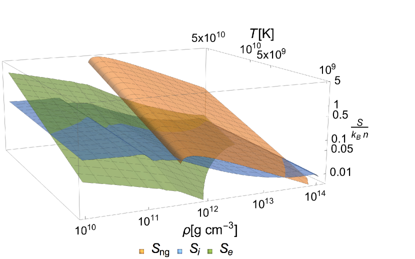
Figure 5: A three-dimensional version of figures 3 and 4, giving fuller information about the dependence of the ion, electron and neutron-gas entropy components as functions of density and temperature.

We conclude with a three-dimensional plot showing the behaviour of the three entropy components as a function of $T$ and $\rho$, giving a better qualitative picture of when different components dominate. We expect a realistic envelope temperature profile to decrease from $\;\raise 1.29167pt\hbox{$>$\kern-7.5pt\raise-4.73611pt\hbox{$\sim$}}\;10^{10}$ K at $\rho_{\rm cc}$ to $\;\raise 1.29167pt\hbox{$<$\kern-7.5pt\raise-4.73611pt\hbox{$\sim$}}\;10^{9}$ K at $\rho=10^{10}\textrm{g cm}^{-3}$ (i.e. lines running from the far right to the near left of the plot). For such profiles, the electron entropy can be neglected throughout the envelope.

We have established that the star’s entropy may reasonably be modelled as due to a single dominant contribution in each region, as we had hoped: the degenerate neutrons in the core, the neutron gas in the inner envelope, and the ions in the outer envelope. This holds for the whole temperature and density range of importance to us here.

2.3 Our simplified thermal model

2.3.1 Isothermal vs isentropic

In general the basic thermodynamic quantities have dependences $S=S(T,\rho)$ and $T=T(S,\rho)$. Assuming that either $S$ or $T$ is constant in some region is very attractive, because it means that the other one of the two quantities must become an explicit function of $\rho$ alone, which makes it far easier to formulate the problem in a manner suitable for an equilibrium solution.

From proto-NS simulations we see that the entropy per baryon $s_{b}$ in the core becomes approximately constant over very few seconds, whereas the temperature varies by a large factor through this region (Burrows & Lattimer, 1986; Pons et al., 1999). For this reason, we will model the core as isentropic with some constant entropy per baryon $s_{b0}$ (in units of $k_{B}$). Since the core makes up most of the star, and will provide the dominant contribution to the star’s thermal pressure, we will treat this region first, and choose a prescription for the envelope regions which matches to the core. Therefore, the fundamental constant for defining the thermal structure of a given stellar model will be $s_{b0}$.

The initial thermal evolution of the outer envelope, above the neutrinospheres, is far faster than that of the neutrino-opaque interior. Being transparent to neutrinos, this region cools rapidly via $e^{-}-e^{+}$ pair annihilation and plasmon decay and reaches an isothermal state. In this work we will assume the outer-envelope temperature to take some fixed value $T_{\rm oe}$ for all our models. Clearly we can typically expect there to be a substantial jump between this value and the temperature as calculated on the inner side of the envelope-core boundary

$$T_{\rm core}(\rho=\rho_{\rm cc})\gg T_{\rm oe}$$ (36)

where matter continues to be heated by the trapped neutrinos.

We will therefore need to construct a transition region that leads us smoothly from the thermal structure of the outer core to that of the outer envelope, similar to the approach employed in Goussard et al. (1997). The simplest resolution to the problem – given that we will need equations in closed form for our iterative method (see section 5) – is to construct some simple closed-form function for either the entropy or the temperature in the inner envelope, to match both to the core and outer-envelope thermal structure. Experimenting with both possibilities, we have found that prescribing $s_{b}$ in the inner envelope in terms of some given function $s_{\rm ie}(\rho)$ and using this to calculate $T$ leads to smaller errors than the other way around, and so we adopt this approach.

In summary, then, our model for the thermal part of the equation of state is the following:
(a) isentropic core, $\rho\geq\rho_{\rm cc}$, entropy due solely to degenerate neutrons;
(b) inner envelope, $\rho_{\rm nd}<\rho<\rho_{\rm cc}$, with entropy per baryon given by some fixed function $s_{\rm ie}(\rho)$, and $T$ calculated from this. Entropy is assumed to be due to the neutron-gas contribution alone;
(c) isothermal outer envelope, $\rho\leq\rho_{\rm nd}$, with some fixed $T_{\rm oe}$, and entropy due to the ion contribution alone.

The exact functional forms of the temperature, entropy and thermal pressure will be discussed in section 4. The model will not make sense once the typical internal temperature drops to $T\sim T_{\rm oe}$, but by that point the thermal contribution to the pressure, and hence to the magnetic-field distribution, will have become negligible.

2.4 Choosing outer-envelope temperature

There appears to be very little discussion in the literature on the temperature of the outer envelope. Goussard et al. (1997) took $T_{\rm oe}=0.2\ \textrm{MeV}=2.3\times 10^{9}$ K, without providing any physical justification for this particular value. Studies on proto-NS structure tend to use enclosed mass as the radial coordinate, thus squashing the entire low-mass envelope into a very thin shell; no detailed information can be gleaned from such plots. It is clear, however, that the outer envelope cools earlier and faster than the initially neutrino-opaque core – and should therefore be assigned a far lower temperature.

For simplicity, and for consistency with our neglect of the electron entropy, we take $T_{\rm oe}=10^{9}$ K in all our models. Note that our results are almost completely independent of any choice less than roughly $10^{10}$ K; the outer envelope has little influence on the structure of the star or its magnetic field. The main rationale is to impose the expected substantial drop in temperature between the core and the outermost regions, and to avoid numerical issues related to finding a suitable inner-envelope function to lead fairly smoothly between the core and outer-envelope thermal structure (we take a quadratic in $\rho$, built assuming the former is considerably bigger than the latter).

3 Equilibrium equations

3.1 Governing equations

Our model of the late stages of a proto-neutron star simply applies the equations of magnetohydrodynamics to a rotating, self-gravitating fluid body in equilibrium. The major novelty of our work is the inclusion of a thermal-pressure term, which is conceptually simple but complex in its details. To avoid additional difficulty we will work in Newtonian gravity, even though a quantitative treatment of a NS should clearly employ general relativity.

Firstly, the force balance in the star is described by the Euler equation:

$$-\frac{1}{\rho}\nabla P-\nabla\Phi+\nabla\Phi_{r}+\frac{1}{4\pi\rho}(\nabla\times{\boldsymbol{B}})\times{\boldsymbol{B}}=0,$$ (37)

where $P$ is the (total) fluid pressure, $\Phi$ the gravitational potential, ${\boldsymbol{B}}$ the magnetic field and

$$\Phi_{r}=\frac{1}{2}r^{2}\sin^{2}\theta\Omega^{2}$$ (38)

the rotational potential, with rigid rotation at frequency $\Omega$ assumed here. The Euler equation is coupled to Poisson’s equation:

$$\nabla^{2}\Phi=4\pi G\rho.$$ (39)

We also need to satisfy the solenoidal constraint

$$\nabla\cdot{\boldsymbol{B}}=0.$$ (40)

The Euler equation has the same form as for previous studies of zero-temperature neutron-star models. Here, however, the pressure has two contributions: one from the degeneracy pressure (which is entirely dominant in cold neutron stars), and a second thermal-pressure term. We assume these two are separable, so that the total fluid pressure is the sum of these, $P=P_{0}+P_{\rm th}$.

3.2 Equilibrium equation of state

The above system of equations is closed by an equation of state for the stellar matter. Models of matter in mature neutron stars generally posit an explicit relation of the form

$$P=P(\rho)$$ (41)

– a barotropic equation of state, for which pressure is no longer an independent variable. With the additional assumption of axisymmetry, this leads to the magnetic field being described by a single PDE of one variable: the Grad-Shafranov equation (Grad & Rubin, 1958; Shafranov, 1958).

On the other hand, Reisenegger (2009) argues that the stratification of matter – due to the presence of either thermal or composition gradients – means that the barotropic relation must be abandoned; the pressure is no longer slave to the density, but can have a more general dependence:

$$P=P(\rho,x_{\mathrm{p}},T,\dots).$$ (42)

This removes a key step in deriving the Grad-Shafranov equation, leading to additional terms that complicate the calculation of equilibria. However, the result is typically wielded in a far stronger way: to state that there is no restriction at all on the magnetic field (Glampedakis & Lasky, 2016), except the usual solenoidal constraint. Were this to be true, the Grad-Shafranov equation could be abandoned, and the magnetic field structure be chosen at will, with the assumption that buoyancy would provide whatever force necessary to satisfy the equilibrium condition – as done by, e.g., Mastrano et al. (2011) and Akgün et al. (2013). Whilst Reisenegger (2009) does argue for an upper limit, $B\sim 10^{17}$ G, to the ability of buoyancy forces to act in this way, none of the models constructed in this manner make a quantitative treatment of the effect of buoyancy forces or check, ex post facto, what kind of force is being implicitly assumed to keep the star in equilibrium, and whether it is consistent with physically-motivated equations of state.

There is, however, another implicit assumption in equation (42), namely that reactions are slow enough that the composition can be ‘frozen’ in and act as an additional variable when determining the pressure. If, however, reactions are fast enough, they will push the system towards beta equilibrium, and the proton fraction (or however else the composition is quantified) will be a function of $\rho$ alone, making the equation of state barotropic for this purpose.

In the first stages of the proto-neutron star evolution, whilst the matter is still opaque to neutrinos, the beta equilibration timescale $\tau_{\beta}\ll\tau_{A}$ except in a very thin shell close to the surface, where the two timescales are comparable (Camelio et al., 2017), and the star can always be considered to be in beta equilibrium for our analysis. Once the core has cooled below $T\approx 5\times 10^{10}$ K (Pons et al., 1999) and has become transparent to neutrinos, we can assume that standard modified Urca reactions act to restore beta equilibrium, leading to a timescale (Villain et al., 2005)

$$\tau_{\beta}\approx 0.5\left(\frac{T}{10^{10}\;\mbox{K}}\right)^{-6}\left(\frac{\rho}{\rho_{0}}\right)^{1/3}\left(\frac{x_{\mathrm{p}}}{0.01}\right)^{1/3}\;\mbox{s}\,,$$ (43)

where $\rho_{0}$ is the nuclear saturation density. If nucleonic or hyperonic direct Urca reactions are possible the equilibration timescale will be even shorter, so in general for temperatures $T>10^{10}$ K, such as those we consider in our model, reactions will occur on a faster timescale than the magnetic field can adjust. It is therefore safe to assume that an unmagnetised proto neutron star is in chemical equilibrium (although not, at this early stage, in thermal equilibrium).

The presence of the magnetic field introduces a considerable complication to this discussion. To see this, it is enough to consider a cold NS model composed of neutron, proton and electron fluids and satisfying local charge neutrality $n_{\rm p}=n_{\rm e}$, for which one can show (e.g. Lander et al. (2012)) that:

$$\nabla\left({\mu_{\rm p}+\mu_{\rm e}-\mu_{\rm n}}\right)=\frac{1}{n_{\rm p}}(\nabla\times{\boldsymbol{B}})\times{\boldsymbol{B}}.$$ (44)

When the right-hand side is zero, this reduces to a statement that the fluids are in chemical equilibrium. This equation, therefore, seems to imply that a magnetic field will generally drive a star out of chemical equilibrium by a (small) amount scaling with $B^{2}$. Furthermore, using a toy model of a thin fluxtube rising through hot unmagnetised neutron-star matter, Reisenegger (2009) argued that beta re-equilibration also becomes considerably slower in the presence of a magnetic field. Gusakov et al. (2017) later reached the same conclusion through analysis of the evolution equations for a magnetised multifluid star. They argue that approximations valid for an unmagnetised star are no longer appropriate, and find equilibration timescales of the order of $10^{6}$ yr for the kinds of temperature and field strength we consider here – clearly vastly longer than the duration of the late proto neutron star phase.

If this view is correct, a magnetic field initially out of chemical equilibrium will remain so throughout this early phase, experiencing an additional buoyancy force that is absent from our modelling. The further the magnetised star is from equilibrium, the less reliable our models will be; in the extreme, the (presumably) complex smallscale field generated at birth could be preserved into the mature phase of the star, although we find it more likely that the magnetic field would never take the star far out of chemical equilibrium. Whatever the result of the birth physics, however, in no case would it be appropriate to model this phase simply by ‘choosing’ an arbitrary magnetic-field configuration and invoking buoyancy forces to balance it.

In principle the interplay between a magnetic field and chemical reactions could be studied by some future nonlinear numerical evolutions of the hot, magnetised multifluid neutron star, hopefully providing a definitive resolution of the issue. In the absence of such a study, we regard our approach as a sensible start. If nothing else, our results represent whatever subclass of proto-neutron-star magnetic fields that do not drive the star out of beta equilibrium. If a magnetised neutron star leaves the birth phase already close to chemical equilibrium, such models may be accurate enough.

Returning to the pressure-density relation and with our assumption that the pressure is separable, we may very generally write:

$$P(\rho,x_{\mathrm{p}},s,T)=P_{0}(\rho,x_{\mathrm{p}})+P_{\rm th}(\rho,s,T,x_{\mathrm{p}}).$$ (45)

However, in chemical equilibrium $x_{\mathrm{p}}=x_{\mathrm{p}}(\rho)$, and since any convective circulation of matter will already have ceased, we can expect thermodynamic quantities to be constant along isopycnic contours, i.e. $T(\rho),s_{b}(\rho)$. In this work we will adopt a model where either $s_{b}$ or $T$ is a prescribed function of $\rho$ in each region, so that the other quantity may then be calculated from this, and will also be a function of $\rho$. As a result, finally, we find that the equation of state will return to being barotropic:

$$P=P(\rho,T(s(\rho)),s(T(\rho)))=P(\rho).$$ (46)

As the star cools below $T\approx 10^{10}$ K, the reaction and Alfven crossing timescales become comparable, and deviations from chemical equilibrium and magnetic effects can balance each other, as predicted by equation (42). However the strong dependence on temperature of the timescale in (43) means that the star rapidly enters the frozen regime, in which the field simply adapts to the fluid configuration as it relaxes. We thus expect any modest deviation from a barotropic equilibrium to be washed out on an equilibration timescale of a few minutes as the star cools, unless some other physical mechanism is at work to maintain this out-of-equilibrium state (see, e.g., Ofengeim & Gusakov (2018) and Castillo et al. (2020) for some recent modelling of magnetic-field evolution during this later phase). Note that our conclusions only apply to quasi-stationary situations: thermal or composition gradients are clearly important actors in proto-NS dynamics, such as the study of oscillation modes.

For the cold part of the EOS, the majority of studies of NS magnetic equilibria have assumed a single polytrope to govern the pressure-density relation, which is a poor reflection of the real star (see however Kiuchi & Kotake (2008) for an exception to this). As a minimal, but physically well-motivated, extension to this, we will take a two-piece polytropic equation of state, with the core and envelope regions having different polytropic indices:

$$P=\begin{cases}k_{1}\rho^{1+1/N_{1}}\textrm{ in envelope, i.e. }\rho<\rho_{\rm cc}\\ k_{2}\rho^{1+1/N_{2}}\textrm{ in core, i.e. }\rho\geq\rho_{\rm cc}.\end{cases}$$ (47)

Continuity and thermodynamic consistency mean that $k_{1}$ and $k_{2}$ are not independent of one another (Read et al., 2009).

4 The thermal pressure

4.1 Non-dimensionalising

For zero-temperature stellar models in Newtonian gravity, it is natural to use combinations of $G$, the central density $\rho_{c}$ and the equatorial radius $R_{*}$ to make all quantities dimensionless. This both simplifies the solution method and ensures that quantities are all (very broadly) of order unity, which decreases the error in numerical calculations. Because quantities like the polytropic constant $k$ drop out from the dimensionless solution, results can be rescaled to any desired stellar model by using the requisite values of $\rho_{c}$ and $R_{*}$ to restore the dimensions $\mathsf{M},\mathsf{L},\mathsf{T}$.

Now that we have thermal quantities, however, we need an extra quantity including the temperature dimension $\mathsf{O}\!\!\!\!-$, in order to make everything dimensionless. We will find that results for hot models will no longer be rescalable.

Note that for supernovae and proto-neutron stars it is convenient to work with the entropy per baryon $s_{b}$, in units of the Boltzmann constant $k_{B}$. $s_{b}$ is dimensionless and is related to the entropy density $S$ through:

$$s_{b}=\frac{\mathcal{S}}{k_{B}\mathcal{N}}=\frac{\mathcal{S}/V}{k_{B}\mathcal{N}/V}=\frac{S}{k_{B}n},$$ (48)

where $\mathcal{S}$ is the entropy and $\mathcal{N}$ the number of particles within some region. Let us use $k_{B}/m_{\rm u}$ as our fourth quantity for nondimensionalising; we see it includes the desired dimension of temperature, since

$$[k_{B}/m_{\rm u}]=[\mathcal{S}]\mathsf{M}^{-1}=\mathsf{L}^{2}\mathsf{T}^{-2}\mathsf{O\!\!\!\!-}^{-1}.$$ (49)

The dimensionless entropy density is then given by:

$$\hat{S}=\frac{S}{(k_{B}/m_{\rm u})\rho_{c}}.$$ (50)

Conveniently, $S/\rho$ in dimensionless units is then given by:

$$\frac{\hat{S}}{\hat{\rho}}=\frac{Sm_{\rm u}}{k_{B}\rho_{c}}\frac{\rho_{c}}{\rho}=\frac{Sm_{\rm u}}{k_{B}\rho}=s_{b},$$ (51)

the entropy per baryon in units of $k_{B}$. Next we need to find the temperature in dimensionless units. Using the dimensions of $k_{B}/m_{\rm u}$ above, and the fact that

$$[G\rho_{c}]=\mathsf{T}^{-2},$$ (52)

we see that the following combination of quantities has dimensions of temperature:

$$(k_{B}/m_{\rm u})^{-1}G\rho_{c}R_{*}^{2}$$ (53)

and so

$$\hat{T}=\frac{k_{B}T}{m_{\rm u}G\rho_{c}R_{*}^{2}}.$$ (54)

We are using $m_{\rm u}$ (the atomic mass unit) instead of the neutron mass, although our core model only considers the thermal contribution of the neutrons.

Not everything in dimensionless form can be rescaled at will, however. The Fermi temperature $T_{\textrm{F}}$ depends on the Fermi energy $\varepsilon_{\textrm{F}}$, which in turn depends on the physical value of density within the star (not just at the centre). This means that we will not be able to remove all physical quantities from our unit system (even though we have got rid of $G$ and $k_{B}/m_{\rm u}$). We will see that this is not a problem for obtaining solutions, but it does mean we will have to specify some stellar quantities in advance, in physical units. In fact, even cold models with our new EOS will be specific to one stellar model, since at least two densities enter the calculation: at the centre and at the transition between different adiabatic indices. We are still able to choose dimensionless units such that $\hat{\rho}=\rho/\rho_{c}$, but having any kind of internal transition at some given physical density clearly means the physical central density must be specified in our dimensionless scheme.

4.1.1 Core

In order to find the thermal-force scalar $\Theta$ we first need an expression for the thermal pressure in convenient, dimensionless form. Comparing the expressions for $P_{\rm th}$ and $S$ from section 2.1.1, we see that

$$P_{\rm th}=\frac{1}{3}ST.$$ (55)

In dimensionless units,

$$\hat{P}_{\rm th}=\frac{1}{3}\frac{\hat{S}}{\hat{\rho}}\hat{\rho}\hat{T}=\frac{1}{3}s_{b}\hat{\rho}\hat{T}.$$ (56)

To use this expression, we need to know the relation between $s_{b}$ and $\hat{T}$. From 2.1.1 we see that

$$s_{b}=\frac{\hat{S}}{\hat{\rho}}=\frac{\pi^{2}}{2}\frac{k_{B}T}{\varepsilon_{\textrm{F}}},$$ (57)

using $n=\rho/m_{\rm u}$ and $\varepsilon_{\textrm{F}}=k_{B}T_{\textrm{F}}$. Now, the Fermi energy is given by

$$\varepsilon_{\textrm{F}} =58.44\left({\frac{n}{n_{0}}}\right)^{2/3}\textrm{ MeV}$$

$$=9.363\times 10^{-5}\left({\frac{\rho}{\rho_{c}}}\right)^{2/3}\left({\frac{\rho_{c}}{\rho_{\rm nuc}}}\right)^{2/3}\textrm{ erg}$$

$$=9.363\times 10^{-5}\hat{\rho}_{\rm nuc}^{-2/3}\hat{\rho}^{2/3}\textrm{ erg},$$ (58)

where $\rho_{\rm nuc}=2.8\times 10^{14}\textrm{g cm}^{-3}$ is nuclear mass density. Using the above expression for $\varepsilon_{\textrm{F}}$ in equation (57) and rearranging, we see that the dimensionless temperature is given by

$$\hat{T} =\frac{k_{B}}{m_{\rm u}G\rho_{c}R_{*}^{2}}\frac{2}{\pi^{2}}\frac{\varepsilon_{\textrm{F}}}{k_{B}}s_{b}$$

$$=0.1712\left({\frac{\rho_{c}}{10^{15}\textrm{ g cm}^{-3}}}\right)^{-1}\left({\frac{R_{*}}{10^{6}\textrm{ cm}}}\right)^{-2}\hat{\rho}_{\rm nuc}^{-2/3}s_{b}\hat{\rho}^{2/3}.$$ (59)

It was not necessary to specify $\rho_{c}$ in advance for earlier, zero-temperature equilibria (Tomimura & Eriguchi, 2005; Lander & Jones, 2009), but since we need the ratio $\rho_{\rm nuc}/\rho_{c}$ here, it is clear that we must now work with the central density in physical units for each model.

We now turn to the thermal-pressure force. This takes the dimensionless form:

$$\nabla\hat{\Theta}=\frac{\nabla\hat{P}_{\rm th}}{\hat{\rho}}=\frac{1}{3\hat{\rho}}\nabla(\hat{\rho}\hat{T}s_{b}).$$ (60)

Since we know that $\hat{\Theta}=\hat{\Theta}(\hat{\rho})$, the thermal force above may be written, using the chain rule, as

$$\nabla\hat{\Theta}(\rho)=\hat{\Theta}^{\prime}\nabla\hat{\rho}=\frac{1}{3\hat{\rho}}\left({\hat{\rho}\hat{T}s^{\prime}_{b}+\hat{\rho}\hat{T}^{\prime}s_{b}+\hat{T}s_{b}}\right)\nabla\hat{\rho}$$ (61)

where all primes denote differentiation with respect to $\hat{\rho}$. Next, note that $\nabla\rho\neq 0$ throughout the star except for its exact centre, and that at the centre itself we must have $\nabla\Theta=0$ for regularity. Therefore we may cancel the $\nabla\hat{\rho}$ terms from the LHS and RHS of the above expression and integrate, to yield

$$\hat{\Theta}=\frac{1}{3}\int\left({\hat{T}s^{\prime}_{b}+\hat{T}^{\prime}s_{b}+\frac{\hat{T}s_{b}}{\hat{\rho}}}\right)\ \mathrm{d}\hat{\rho},$$ (62)

which will include some integration constant. There should be freedom in choosing this constant, since the physical equilibrium of the star depends only on $\Theta^{\prime}(\rho)$ and not $\Theta$ itself; it is like a gauge freedom. This will be useful to us later.

To evaluate $\Theta$ in general, we would need both $S$ and $T$ inputs from numerical simulations of the late proto-neutron-star phase. However, as discussed in 2.3.1 , we will adopt a simplified model that avoids this requirement. In our model the core is assumed to be isentropic:

$$s_{b} =s_{b0}=\frac{\hat{S}}{\hat{\rho}}$$ (63)

$$\hat{T} =0.1697\left({\frac{\rho_{c}}{10^{15}\textrm{ g cm}^{-3}}}\right)^{-1}\left({\frac{R_{*}}{10^{6}\textrm{ cm}}}\right)^{-2}\hat{\rho}_{\rm nuc}^{-2/3}s_{b0}\hat{\rho}^{2/3}.$$ (64)

We now have $T$ as a function of $\rho$, and so

$$\hat{\Theta}=\frac{1}{3}\int\left({\hat{T}^{\prime}s_{b}+\frac{\hat{T}s_{b}}{\hat{\rho}}}\right)\ \mathrm{d}\hat{\rho},$$ (65)

using the isentropic assumption $s^{\prime}_{b}=0$. Integrating the above, we have

$$\hat{\Theta}=\frac{5}{6}s_{b0}\hat{T}.$$ (66)

We now move on to calculating the thermal-pressure force in the envelope regions for our model.

4.1.2 Outer envelope

As discussed in section 2.3.1, we take the outer envelope to be isothermal with some fixed physical temperature $T_{\rm oe}$ in kelvin for all stellar models (except the zero-temperature models we compare with in the results section). We first convert this to a non-dimensional value using equation (54); unlike the physical value, this will vary between models.

We have established that the thermal structure is dominantly due to the ions. The dimensionless thermal pressure for a Boltzmann gas of ions is

$$\hat{P}_{\rm th}=\frac{n_{\rm i}k_{B}T}{G\rho_{c}^{2}R_{*}^{2}}=\frac{\hat{\rho}\hat{T}}{A},$$ (67)

using the fact that $A^{\prime}=A$ in the outer envelope. From the above we calculate the form of the thermal-pressure scalar:

$$\hat{\Theta} =\int\frac{1}{\hat{\rho}}\frac{\mathrm{d}{\hat{P}_{\rm th}}}{\mathrm{d}{\hat{\rho}}}\ \mathrm{d}\hat{\rho}$$

$$=\frac{1}{A}\int\left({\frac{\hat{T}}{\hat{\rho}}+\frac{\mathrm{d}{\hat{T}}}{\mathrm{d}{\hat{\rho}}}}\right)\ \mathrm{d}\hat{\rho},$$ (68)

where we have assumed for simplicity that $A$ is constant in the region of interest to us (i.e. the inner part of the outer envelope); we take $A=100$ as a representative value for this region.

For an isothermal envelope we then have

$$\hat{\Theta}=\frac{\hat{T}_{\rm oe}\ln\hat{\rho}}{A}.$$ (69)

This is only evaluated within the star and not at the surface, so no issues arise from the divergent nature of this expression for $\rho\to 0$.

For the purposes of the equilibrium calculation, the ion entropy is not used explicitly to derive the thermal-pressure scalar. We will however need it in order to construct an entropy function for the inner envelope; see next. Equation 22 gives the entropy density per ion. To convert to an entropy per baryon (in units of $k_{B}$), we divide the dimensionless form of this entropy by $\hat{\rho}$, to give:

$$s_{b}=\frac{\hat{S}_{\rm i}}{\hat{\rho}} =\frac{1}{A}\left[\frac{5}{2}-\ln(n_{\rm i}\lambda_{\rm i}^{3})\right]$$

$$=\frac{1}{100}\left[\frac{5}{2}-\ln\left({4.47\times 10^{-5}\rho_{c,15}^{-1/2}R_{6}^{-3}}\right)-\ln\left({\hat{\rho}\hat{T}^{-3/2}}\right)\right],$$ (70)

where we evaluate the expression for $A=100$ on the second line.

4.1.3 Inner envelope

With the above expression, we evaluate the entropy per baryon at the inner edge of the outer envelope $s_{\rm oe}$. The value in the core is also known, and fixed at $s_{b0}$ from the outset of the calculation. We now construct a quadratic function $s_{\rm ie}$ for the entropy per baryon in the inner envelope to lead between these two values:

$$s_{\rm ie}(\hat{\rho})=s_{b0}-\frac{(s_{b0}-s_{\rm oe})}{(\hat{\rho}_{\rm cc}-\hat{\rho}_{\rm nd})^{2}}(\hat{\rho}_{\rm cc}-\hat{\rho})^{2}.$$ (71)

Using this prescription gives us models where $s_{b}$ throughout the star is continuous and quite smooth.

In the inner envelope we assume that only the neutron gas contributes to the thermal structure. This is physically the same as in the core, except that number density factors $n$ are weighted with a prefactor

$$\xi\equiv\frac{X_{\rm n}}{(1-u)}$$ (72)

that determines the microscopic density of the degenerate neutron gas outside nuclei within the region. The thermal pressure takes the same form as in the core, equation (55), except that the relation between the entropy and the temperature is now given by

$$s_{b}=s_{\rm ie}(\hat{\rho})=\frac{\hat{s}_{\rm ng}}{\hat{\rho}}=\frac{\pi^{2}}{2}\xi\frac{k_{B}T}{\varepsilon_{\textrm{F}}}.$$ (73)

Through its density term, the Fermi energy (58) in the inner envelope picks up a prefactor $\xi^{2/3}$. Rearranging for the dimensionless temperature as in the core case, then, we arrive at the same expression as equation (59), but with a prefactor of $\xi^{-1/3}$:

$$\hat{T}=0.1712\left({\frac{\rho_{c}}{10^{15}\textrm{ g cm}^{-3}}}\right)^{-1}\left({\frac{R_{*}}{10^{6}\textrm{ cm}}}\right)^{-2}\hat{\rho}_{\rm nuc}^{-2/3}\xi^{-1/3}s_{b}\hat{\rho}^{2/3}.$$ (74)

The presence of $\xi$ is a considerable complicating factor in our calculation. In problems where a quantitative treatment of inner-envelope physics is required (e.g. for pulsar glitches), it is clearly important. Note, however, that for almost the whole density range of the inner envelope $\xi\approx 0.6-0.8$, corresponding to a prefactor $\xi^{-1/3}\approx 1.1-1.2$ in the above equation. Only in the region $3.5\times 10^{11}<\rho[\textrm{g cm}^{-2}]\;\raise 1.29167pt\hbox{$<$\kern-7.5pt\raise-4.73611pt\hbox{$\sim$}}\;2\times 10^{12}$ does $\xi$ have larger variation – but this corresponds to, at most, a very few grid points for us.

We have experimented with different prescriptions for $\xi$, finding that the mismatch at the envelope-core boundary for $\xi\neq 1$ introduces considerable error (in the sense of not satisfying the virial test of section 6 to high precision), but with imperceptible changes in the actual stellar models. For this reason we will make the simplification, from now on, that $\xi=1$ throughout the inner envelope. Since the entropy is a prescribed function $s_{\rm ie}(\hat{\rho})$, the inner-envelope temperature can then be calculated from

$$\hat{T} =0.1712\left({\frac{\rho_{c}}{10^{15}\textrm{ g cm}^{-3}}}\right)^{-1}\left({\frac{R_{*}}{10^{6}\textrm{ cm}}}\right)^{-2}\hat{\rho}_{\rm nuc}^{-2/3}s_{\rm ie}(\hat{\rho})\hat{\rho}^{2/3}$$

$$\equiv\mathfrak{c}s_{\rm ie}(\hat{\rho})\hat{\rho}^{2/3},$$ (75)

where we have defined the constant $\mathfrak{c}$ to absorb the various numerical prefactors above. We may now calculate the thermal-force scalar in the inner envelope:

$$\hat{\Theta} =\frac{1}{3}\int\left({\hat{T}s^{\prime}_{\rm ie}+\hat{T}^{\prime}s_{\rm ie}+\frac{\hat{T}s_{\rm ie}}{\hat{\rho}}}\right)\ \mathrm{d}\hat{\rho}$$

$$=\frac{\mathfrak{c}}{3}\left[s_{\rm ie}^{2}\hat{\rho}^{2/3}+\int s^{2}_{\rm ie}\hat{\rho}^{-1/3}\ \mathrm{d}\hat{\rho}\right]$$

$$=\frac{\mathfrak{c}\hat{\rho}^{2/3}s_{\rm ie}}{3}\left[s_{\rm ie}+\frac{f(\hat{\rho})}{s_{\rm ie}}\right]$$

$$=\frac{\hat{T}}{3}\left[s_{\rm ie}+\frac{f(\hat{\rho})}{s_{\rm ie}}\right],$$ (76)

where $f(\hat{\rho})$ is a rather messy quartic in $\hat{\rho}$ emerging from the above integration.

4.1.4 Matching $\Theta$ contributions

The freedom to choose the integration constant for $\Theta$ in each region means we are able to adjust these to produce a continuous, quite smooth, $\Theta$ profile from the centre to the surface of the star. In particular, let $\Theta_{\rm core},\Theta_{\rm ie},\Theta_{\rm oe}$ denote the functions from equations (66), (76), (69) without integration constants added on. For the core we choose $\Theta=\Theta_{\rm core}$, i.e. without integration constant. We then move to the inner envelope, creating a function $\tilde{\Theta}_{\rm ie}$ that matches to $\Theta_{\rm core}$ at the envelope-core boundary, and then create an adjusted outer-envelope function $\tilde{\Theta}_{\rm oe}$ to match to this $\tilde{\Theta}_{\rm ie}$ at the inner-outer envelope boundary. For all points with $\rho=0$, $\Theta$ is taken to have the value $\tilde{\Theta}_{\rm oe}^{\rm surf}$ obtained from evaluating $\tilde{\Theta}_{\rm oe}$ at the last gridpoint within the star. To summarise, then,

$$\Theta(\rho)=\begin{cases}\Theta_{\rm core}(\rho)&\rho\geq\rho_{\rm cc}\\ \Theta_{\rm ie}(\rho)-\Theta^{\rm cc}_{\rm ie}+\Theta^{\rm cc}_{\rm core}\equiv\tilde{\Theta}_{\rm ie}(\rho)&\rho_{\rm nd}<\rho<\rho_{\rm cc}\\ \Theta_{\rm oe}(\rho)-\Theta^{\rm nd}_{\rm oe}+\tilde{\Theta}^{\rm nd}_{\rm ie}\equiv\tilde{\Theta}_{\rm oe}(\rho)&0<\rho\leq\rho_{\rm nd}\\ \tilde{\Theta}_{\rm oe}^{\rm surf}&\rho=0\end{cases}$$ (77)

where the superscripts cc and nd denote quantities evaluated at $\rho=\rho_{\rm cc}$ and $\rho_{\rm nd}$ respectively.

5 Numerical solution method

A large number of previous studies have solved for magnetic-field equilibrium models in NSs using numerical iterative schemes; of particular note are the first solutions for a linked poloidal-toroidal field in Newtonian gravity (Tomimura & Eriguchi, 2005) and full general relativity (Uryū et al., 2019). As in Tomimura & Eriguchi (2005), we will employ the Hachisu self-consistent field (HSCF) method (Hachisu, 1986), a robust iterative procedure that has several advantages over perturbative methods: one can solve for models up to Keplerian rotation rates, with extremely strong magnetic fields, and include the contributions from high multipoles in the solution without significant extra difficulty. The resulting models are true self-consistent equilibria; whilst perturbative studies account for the effect of the fluid distribution on the magnetic field, a numerical iterative method is also able to account for the back-reaction of the field on the fluid. Complementary to these magnetised models, there has been a limited amount of research on the construction and use of self-consistent methods to build hot, rotating and unmagnetised stellar models (Jackson et al., 2005; Goussard et al., 1997; Camelio et al., 2019). We will build on this body of work to produce models of hot NSs with magnetic fields.

The HSCF method is semi-analytic, in that it exploits certain closed-form expressions for the fluid and magnetic field in order to iterate towards an equilibrium solution. These are valid for cold polytropic stellar models; in the following we check whether they can be adapted for models with a more realistic description of the pressure in a hot proto neutron star: including both a model of the thermal pressure, and a piecewise-polytropic description of the degeneracy-pressure profile.

5.1 Iterative solution: the fluid distribution

5.1.1 First-integral form of the Euler equation

Firstly, we need to be able to write the Euler equation in integral form. We have argued that the zero-$T$ part of the EOS is barotropic, $P_{0}=P_{0}(\rho)$, meaning that one can write:

$$\frac{\nabla P_{0}}{\rho}=\nabla H,$$ (78)

where $H$ is the enthalpy per unit mass, and is found from the integral:

$$H=\int\limits_{0}^{P_{0}}\frac{\mathrm{d}\tilde{P}}{\rho(\tilde{P})},$$ (79)

where the tildes denote dummy integration variables. Here we have used the enthalpy, whereas some other papers use the chemical potential per unit mass,

$$\tilde{\mu}\equiv\frac{\mu}{m}.$$ (80)

Provided that we are able to separate out thermodynamic quantities into zero- and finite-temperature pieces, the two are equivalent. We can see this from the Euler relation:

$$\tilde{\mu}=\frac{\mu}{m}=\frac{U+P-sT}{mn} =\frac{1}{\rho}(U_{0}+P_{0}+U_{\rm th}+P_{\rm th}-sT)$$

$$=H_{0}+\frac{1}{\rho}(U_{\rm th}+P_{\rm th}-sT),$$ (81)

using the definition of $H$. Thus, at zero temperature there is no distinction between $H$ and $\tilde{\mu}$.

Using $H$, the Euler equation for a cold star becomes:

$$\nabla(H+\Phi-\Phi_{r})=\frac{1}{4\pi\rho}(\nabla\times{\boldsymbol{B}})\times{\boldsymbol{B}}.$$ (82)

Finally, if we take the curl of this we see that

$$\nabla\times\left[\frac{1}{4\pi\rho}(\nabla\times{\boldsymbol{B}})\times{\boldsymbol{B}}\right]=0\implies\frac{1}{4\pi\rho}(\nabla\times{\boldsymbol{B}})\times{\boldsymbol{B}}=\nabla M$$ (83)

for some scalar function $M$. We then arrive at an important result for the HSCF scheme: that the Euler equation becomes a Bernoulli equation, and therefore may immediately be expressed in first-integral form:

$$H+\Phi-\Phi_{r}-M=C,$$ (84)

where $C$ is an integration constant, which is fixed through boundary conditions at the surface.

The thermal quantities $T$ and $S$ are also functions of $\rho$ in our model, and as a result the thermal pressure force may be written

$$\frac{\nabla P_{\rm th}}{\rho}=\nabla\Theta.$$ (85)

As a result, the Euler equation (84) may trivially be generalised to:

$$H+\Theta+\Phi-\Phi_{r}-M=C.$$ (86)

Now, using the explicit form of $\Phi_{r}$, we have:

$$H+\Theta+\Phi-\frac{\Omega^{2}}{2}r^{2}\sin^{2}\theta-M=C,$$ (87)

and we define the surface as being where

$$H=0.$$ (88)

It would be most natural to define it as being where the density drops to zero instead, but this is not convenient for numerical implementation. So, evaluating the above Euler equation at the polar and equatorial surfaces – in code units where the equatorial surface is at $\hat{r}_{\rm eq}=\hat{R}_{*}=1$ – we have

$$\hat{\Theta}(\hat{r}_{\rm pole})+\hat{\Phi}(\hat{r}_{\rm pole})-\hat{M}(\hat{r}_{\rm pole}) =\hat{C},$$ (89)

$$\hat{\Theta}(1)+\hat{\Phi}(1)-\frac{\hat{\Omega}^{2}}{2}-\hat{M}(1) =\hat{C},$$ (90)

Subtracting the second equation from the first gives us an expression for the rotation rate:

$$\hat{\Omega}^{2}=2[\hat{\Phi}(1)-\hat{\Phi}(\hat{r}_{\rm pole})]-2[\hat{M}(1)-\hat{M}(\hat{r}_{\rm pole})],$$ (91)

where the $\hat{\Theta}$ terms cancel, since the function is constant along any density contour (in this case, the $\hat{\rho}=0$ contour). Now that we have $\hat{\Omega}$ we may also use either of the above boundary equations to calculate $C$.

5.1.2 Iterative method: second key step

The second important requirement of the HSCF method is the ability to find a closed-form inversion for $\rho=\rho(H)$. This is only true for particular special choices of the EOS, like a polytrope:

$$P=k\rho^{\gamma}=k\rho^{1+1/N}.$$ (92)

For this polytropic EOS a straightforward integration, using equation (79), shows that

$$H=k(1+N)\rho^{1/N},$$ (93)

which can be rearranged to give

$$\rho=\left({\frac{H}{k(1+N)}}\right)^{N}.$$ (94)

This is effectively the iterative step for the method, used to find a new density distribution – one closer to an equilibrium state than the previous one.

Now, if we work in dimensionless units by dividing all physical quantities by combinations of the central density $\rho_{c}$, stellar radius $R_{*}$ and the gravitational constant $G$, we can make the expressions even simpler. Evaluating (93) at the centre of the star in dimensionless units, we have:

$$\hat{H}_{c}=\hat{k}(1+N)\hat{\rho}_{c}^{1/N}=\hat{k}(1+N),$$ (95)

where hats denote dimensionless variables, and where we have used $\hat{\rho}_{c}=1$. Now substituting this relation into equation (94), we get the very simple result:

$$\hat{\rho}=\left({\frac{\hat{H}}{\hat{H}_{c}}}\right)^{N}.$$ (96)

We have eliminated the polytropic constant $k$ by working in dimensionless units. This means that the final dimensionless model may be redimensionalised to a whole set of models with different $k$, meaning different mass and radius.

5.1.3 Piecewise polytrope

We now generalise the above result to the two-piece polytrope of equation (47). The relevant basic formulae for a relativistic multi-piece polytrope are given in Read et al. (2009). Because we work in Newtonian gravity, however, we have amended the expressions of Read et al. (2009) to remove the relativistic term $\rho c^{2}$ from the energy density.

Firstly, the requirement that the pressure should be continuous across the boundary between the two polytropes means that the two polytropic constants may not be chosen independently. In particular, the internal energy $U(\rho)$ and enthalpy $H(\rho)$ are given by:

$$U(\rho)=\left[\frac{U(\rho_{i-1})}{\rho_{i-1}}-\frac{k_{i}}{(\gamma_{i}-1)}\rho_{i-1}^{\gamma_{i}-1}\right]\rho+\frac{k_{i}}{(\gamma_{i}-1)}\rho^{\gamma_{i}},$$ (97)

$$H(\rho)=\frac{U(\rho_{i-1})}{\rho_{i-1}}-\frac{k_{i}}{(\gamma_{i}-1)}\rho_{i-1}^{\gamma_{i}-1}+\frac{k_{i}\gamma_{i}}{(\gamma_{i}-1)}\rho^{\gamma_{i}-1}.$$ (98)

Since we consider a two-piece polytrope, the transition densities are $\rho_{01}=0$ (the stellar surface) and $\rho_{12}=\rho_{\rm cc}$ (the envelope-core transition). Continuity of pressure at the envelope-core boundary:

$$P=k_{1}\rho_{\rm cc}^{1+1/N_{1}}=k_{2}\rho_{\rm cc}^{1+1/N_{2}}$$ (99)

immediately gives

$$k_{1}=k_{2}\rho_{\rm cc}^{1/N_{2}-1/N_{1}}.$$ (100)

Since $U/\rho\to 0$ at the surface, we find for the envelope:

$$U_{\rm env}(\rho)=\frac{k_{1}}{(\gamma_{1}-1)}\rho^{\gamma_{1}}=k_{2}\rho_{\rm cc}^{1/N_{2}-1/N_{1}}N_{1}\rho^{1+1/N_{1}},$$ (101)

$$H_{\rm env}(\rho)=\frac{k_{1}\gamma_{1}}{(\gamma_{1}-1)}\rho^{\gamma_{1}-1} =(N_{1}+1)k_{1}\rho^{1/N_{1}}$$

$$=(N_{1}+1)k_{2}\rho_{\rm cc}^{1/N_{2}-1/N_{1}}\rho^{1/N_{1}}.$$ (102)

The $U_{\rm env}$ will not be directly used in our solution, but is needed in deriving the enthalpy for the core region:

$$H_{\rm core}(\rho)=k_{2}\left[(N_{1}-N_{2})\rho_{\rm cc}^{1/N_{2}}+(N_{2}+1)\rho^{1/N_{2}}\right].$$ (103)

The central enthalpy, in code units, is therefore

$$\hat{H}_{c}(\rho)=\hat{k}_{2}\left[(N_{1}-N_{2})\hat{\rho}_{\rm cc}^{1/N_{2}}+N_{2}+1\right].$$ (104)

Now dividing the enthalpy by its central value allows us to eliminate explicit mention of the polytropic constant, as in the single-polytrope case. This leads to an inversion of $\hat{\rho}$ in terms of $\hat{H}$ with different forms in each region, as follows:

$$\hat{\rho}_{\rm env}=\hat{\rho}_{\rm cc}\left\{\frac{\left[N_{1}-N_{2}+(N_{2}+1)\hat{\rho}_{\rm cc}^{-1/N_{2}}\right]}{(N_{1}+1)}\frac{\hat{H}_{\rm env}}{\hat{H}_{c}}\right\}^{N_{1}},$$ (105)

$$\hat{\rho}_{\rm core}=\hat{\rho}_{\rm cc}\left\{\frac{\left[N_{1}-N_{2}+(N_{2}+1)\hat{\rho}_{\rm cc}^{-1/N_{2}}\right]}{(N_{2}+1)}\frac{\hat{H}_{\rm core}}{\hat{H}_{c}}-\frac{(N_{1}-N_{2})}{(N_{2}+1)}\right\}^{N_{2}}.$$ (106)

Note that upon setting $N_{1}=N_{2}$, both of the above relations reduce to the single-polytrope case of equation (96), as required.

5.2 Iterative solution: the magnetic field

As mentioned above, for magnetised stellar models the extended HSCF method also requires us to be able to find an integral equation incorporating information about the star’s magnetic field. The description here is breviloquent, since detailed derivations may be found elsewhere (e.g. Lander & Jones (2009)).

If we assume the star to be axisymmetric and work in cylindrical polar coordinates $(\varpi,\phi,z)$ aligned so that the $z$ coordinate is the star’s symmetry axis, then one can show from the constraint $\nabla\cdot{\boldsymbol{B}}=0$ that the magnetic field can be expressed in the form

$${\boldsymbol{B}}={\boldsymbol{B}}_{\rm pol}+{\boldsymbol{B}}_{\rm tor}=\frac{1}{\varpi}\left({\nabla u\times{\bf e}_{\phi}+f(u){\bf e}_{\phi}}\right),$$ (107)

where $u$ is the poloidal magnetic streamfunction, defined through this expression, and $f(u)$ is a function of $u$ – which from a mathematical perspective is virtually arbitrary, but physically relates to the toroidal-field component. In order to avoid toroidal field – and therefore an electric current – outside the star, the function $f$ needs to be fitted to a contour of $u$ which closes within the star. If we define $u_{\rm max}$ as the largest such contour (i.e. the last field line which closes inside the star), then

$$f(u)=a(u-u_{\rm max})^{\zeta}\mathcal{H}(u-u_{\rm max}),\zeta>1,$$ (108)

where $\mathcal{H}$ is the Heaviside function and $a$ and $\zeta$ are constants. It is clear from the form of the Lorentz force that $\nabla M\cdot{\boldsymbol{B}}=0$, and from the expression for ${\boldsymbol{B}}$ in terms of $u$ we also have $\nabla u\cdot{\boldsymbol{B}}=0$. The two gradients $\nabla M$ and $\nabla u$ are therefore parallel, and so we deduce that

$$M=M(u).$$ (109)

One can then derive a single differential equation in the variable $u$, which – together with the chosen prescriptions for $M(u)$ and $f(u)$ – encodes all the information about the magnetic field. This is known as the Grad-Shafranov equation, and has the form:

$$\Delta_{*}u=-4\pi\rho\varpi^{2}\frac{\mathrm{d}{M}}{\mathrm{d}{u}}-f\frac{\mathrm{d}{f}}{\mathrm{d}{u}},$$ (110)

where the differential operator $\Delta_{*}$ is the axisymmetric Laplacian operator, but with the opposite sign on the first-derivative piece:

$$\Delta_{*}\equiv\frac{\partial{{}^{2}}}{\partial{\varpi^{2}}}-\frac{1}{\varpi}\frac{\partial{}}{\partial{\varpi}}+\frac{\partial{{}^{2}}}{\partial{z^{2}}}.$$ (111)

Exploiting a standard Green’s function, equation (110) may be written in a Poisson-like integral form (Tomimura & Eriguchi, 2005; Lander & Jones, 2009), completing the system of integral equations. It needs to be solved to find $u$ at each iterative step, using the $u$ and $\rho$ distributions from the previous step. With the updated solution for $u$, one then evaluates $M(u)$ with it, and uses this in the first integral of the Euler equation. In this way, the magnetic field and the density distribution are self-consistently updated at each iterative step:
(i) we account for the effect of the density distribution and from the different forces in the star on the magnetic field;
(ii) we account for the distortion to the density distribution induced by the magnetic field.

5.2.1 Function choices in this paper

Other than the restrictions described above, the functional forms of $f(u)$ and $M(u)$ may be chosen freely, although varying these has limited effect on the resulting equilibria, if they are found using a self-consistent method; see Lander & Jones (2012) or Bucciantini et al. (2015) for a survey of these parameters. The constant $\kappa$ sets the overall field strength, and $a$ the maximum strength of the toroidal component; the value of $\zeta$ is less important. For all poloidal/linked poloidal-toroidal field results in this paper we take $\zeta=0.01$ and $M(u)=\kappa(u/u_{\rm gmax})^{5}$ (where $u_{\rm gmax}=\max(u)$); we have found that these allow for the maximum strength of toroidal field in our linked poloidal-toroidal magnetic-field solutions (which are always dominated, energetically, by the poloidal component). For purely toroidal fields – a different class of solution where there is no additional equation like equation (110) to solve – we take $M=-\lambda^{2}\rho\varpi^{2}/4\pi$, where $\lambda$ is a constant governing the field strength (Lander & Jones, 2009).

5.3 Physical sequences of models

In cold polytropic models of NSs, one calculates a single dimensionless model (the most natural choice being an unmagnetised non-rotating one), chooses the desired physical mass $\mathcal{M}$, and finds the value of the (single) polytropic constant $k$ that gives the desired physical radius $R_{*}$. Any two models with the same physical $\mathcal{M},k$ can be regarded as the same physical star; we therefore restore the dimensions of other models (rotating and/or magnetised), by multiplying by the requisite combination of $\rho_{c}$ and $R_{*}$ (found from the fixed physical $\mathcal{M},k$ and the dimensionless $\hat{\mathcal{M}},\hat{k}$ calculated for an individual model).

Here, with a two-piece polytrope and hot models, the procedure is less general but similar. We again fix a non-rotating, unmagnetised, and now also zero-$T$ model; in all results reported here this spherical reference model has $\mathcal{M}=1.4\mathcal{M}_{\odot}$, where $\mathcal{M}_{\odot}$ is the mass of the Sun, and $R_{*}=12$ km. We run the code for such a model and obtain the dimensionless polytropic constant $\hat{k}_{2}$ for the core from equation (104) and the dimensionless mass $\hat{\mathcal{M}}$ by volume integration of $\hat{\rho}$. Now, since these two dimensionless quantities are related to their physical counterparts by:

$$\hat{\mathcal{M}}=\frac{\mathcal{M}}{\rho_{c}R_{*}^{3}},\ \hat{k}_{2}=\frac{k_{2}}{G\rho_{c}^{1-1/N_{2}}R_{*}^{2}},$$ (112)

we may combine these relations to calculate the physical value of $k_{2}$ for the reference model:

$$k_{2}=\hat{k}_{2}G\left({\frac{\mathcal{M}}{\hat{\mathcal{M}}}}\right)^{1-1/N_{2}}R_{*}^{3/N_{2}-1}.$$ (113)

Recall that the envelope polytropic constant $k_{1}$ is not independent of $k_{2}$, and hence the corresponding relation for $k_{1}$ gives no additional information. We choose to work with $k_{2}$, as the core comprises most of the mass and volume of the star. A physical sequence of models, therefore, has fixed $k_{2}$ and $\mathcal{M}$ in physical units. Their dimensionless counterparts will, however, vary from model to model depending on the star’s rotation rate, magnetic field and temperature. Using these physical and dimensionless quantities, we are now able to calculate the physical equatorial radius for any given model, through a rearrangement of equation (113):

$$R_{*}=\left[\hat{k}_{2}G\left({\frac{\mathcal{M}}{\hat{\mathcal{M}}}}\right)^{1-1/N_{2}}\right]^{N_{2}/(N_{2}-3)}.$$ (114)

Having done so, we are then able to calculate the central density in physical units:

$$\rho_{c}=\frac{\mathcal{M}}{\hat{\mathcal{M}}R_{*}^{3}}.$$ (115)

Since $\rho_{c}$ enters the iterative procedure for both hot and piecewise-polytropic models, we must recalculate $R_{*}$ and $\rho_{c}$ using the above relations at each iterative step.

5.4 Iterative scheme

The HSCF-based numerical scheme we use iterates towards a solution by using the equilibrium equations in integral form. The scheme takes the form:
0. As initial conditions to start an iteration, make simple trial guesses for $\rho$ and $u$;
1. Calculate the gravitational potential $\Phi$ from the $\rho$ distribution and Poisson’s equation (39) in integral form;
2. Calculate the new magnetic streamfunction $u$ from its previous form $u_{\textrm{old}}$, using the magnetic Poisson equation (110) (in integral form) with $u_{\textrm{old}}$ and $\rho$ in the integrand;
3. Calculate, in physical units, $R_{*}$ and $\rho_{c}$, and use these to calculate the thermal-force scalar $\hat{\Theta}$;
4. Evaluating the Euler equation at the equatorial and polar surfaces, equations (91) and (90), find $\hat{\Omega}^{2}$ and $\hat{C}$;
5. We are now able to use the Euler equation (86) to find $H$ throughout the star;
6. Calculate the new density distribution in the envelope and core with equations (105), (106);
7. For stability reasons we do not always use the fully-updated $u,\rho$ distributions for the following iterative step, but instead employ an underrelaxation step. We then return to step 1 using the partially-updated $\rho$ and $u$ distributions, repeating the cycle until satisfactory convergence is achieved, i.e. until the fractional changes in $\hat{H},\hat{C},\hat{\Omega}^{2},\hat{u}$ between consecutive iterative steps drop below some small tolerance value (usually $10^{-4}-10^{-5}$).

The input parameters for any equilibrium configuration are the surface distortion $r_{\textrm{pole}}/r_{\textrm{eq}}$, the polytropic indices in the core and envelope regions $N_{1},N_{2}$ and prefactors $a,\kappa$ related to the strengths of the poloidal and toroidal field components. In the purely-toroidal case there is a single constant $\lambda$ to specify. The grid is evenly-spaced in $r$ and $\cos\theta$; the latter ensures that the equatorial region is well resolved even with a limited number of angular grid points. This is important since this region can have complex field geometry, with coexisting poloidal and toroidal components, and strong variations in the density for models rotating close to Keplerian velocity – whereas the polar region is relatively featureless. Since the density and physics of the envelope region changes over a radius $\sim 0.1R_{*}$, good coverage of this region is also needed. For these reasons we have found a good grid resolution, which we adopt as our standard here, consists of $512$ radial gridpoints and $128$ angular gridpoints.

The code exploits a decomposition of the governing equations into multipoles. Since the models are axisymmetric the azimuthal index $m$ is zero, and the equations become an infinite expansion in terms of Legendre polynomials with angular index $l$. For numerical purposes this clearly must be terminated at some maximum $l=l_{\rm max}$, at which the contribution of additional multipoles should be negligible. For more extreme models – a very strong toroidal component or very rapid rotation – we have found that very high multipoles can make a visible difference to the final magnetic-field configuration (see section 6.6), and so we choose $l_{\rm max}=32$ as standard in this work.

The iterative process described here typically takes of the order $10-500$ steps, and even for high resolutions finishes within a few minutes when run on a typical laptop. The code is stable up to $s_{b0}=2$ in many cases, and up to $s_{b0}=1.5$ for extremal models (i.e. Keplerian rotation and/or strong magnetic fields); this is certainly adequate, since higher values of entropy are not consistent with our hot EOS model anyway.

6 Results

6.1 Virial test

\psfrag{NDIV}{$N_{\rm DIV}$}\psfrag{VT}{$VT$}\includegraphics[width=433.62pt]{figs/virial.eps}

Figure 6: Convergence of code accuracy with increased resolution, for a hot, rapidly-rotating and highly magnetised model ($s_{b0}=1.0$, $\Omega=690$ Hz, $\hat{\kappa}=0.3,\ \hat{a}=12$). Points show virial-test results $VT$ for different numbers of radial grid points $N_{\rm DIV}$, and the dashed line shows the expected behaviour for a second-order code, of inverse-square scaling with grid resolution.

Before moving to our results, we first confirm that our numerical code is behaving as expected. The natural measure of the accuracy of such a code comes from the virial theorem, in which the vector Euler equation is converted into a scalar energy balance:

$$\mathcal{E}_{\rm grav}+3\Pi_{0}+3\Pi_{\rm th}+2\mathcal{E}_{\rm kin}+\mathcal{E}_{\rm mag}=0,$$ (116)

where $\mathcal{E}_{\rm grav},\mathcal{E}_{\rm kin},\mathcal{E}_{\rm mag}$ are the gravitational binding, kinetic and magnetic energies; and $\Pi_{0},\Pi_{\rm th}$ the volume integrals of the zero-temperature and thermal pressures. In the above form of the virial theorem the right-hand side is zero, reflecting the fact that the solution should be a stationary equilibrium. The left-hand side is evaluated for the solutions produced by the numerical scheme, and then normalised by dividing by $|\mathcal{E}_{\rm grav}|$, to give a dimensionless measure of the code’s accuracy: the virial test $VT$. In figure 6 we present values of $VT$ for a numerically challenging model to calculate (hot, highly-magnetised and rapidly-rotating) as a function of grid resolution. We confirm that the error is very small compared with unity, and furthermore that it drops with increasing resolution in the manner expected for a second-order convergent scheme (the order at which the code is written). For all results presented in this paper the virial test has also been checked; it is never more than order $10^{-4}$, and in many cases is as low as $10^{-6}$, comparing favourably with other studies.

6.2 Keplerian velocity

With progressively more rapid rotation, a star becomes more oblate, until – at some critical rotation rate – it begins to lose mass from the equatorial surface. At this Keplerian rotation rate $\Omega_{K}$ the centrifugal force at the equatorial surface matches the gravitational force, $\nabla\Phi_{r}=\nabla\Phi$. To check when this is reached, we evaluate the auxiliary quantity

$$\Omega_{c}^{2}=\frac{1}{R_{*}}\frac{\partial{\Phi}}{\partial{r}}.$$ (117)

This quantity is generally less than $\Omega^{2}$, but when Keplerian velocity is reached the two become equal: $\Omega_{c}=\Omega=\Omega_{K}$. Models with $\Omega>\Omega_{c}$ are unphysical for our purposes, as the star would be in a dynamical mass-shedding state. Clearly we cannot calculate a model that precisely satisfies the Keplerian condition; instead, we repeatedly run the code to find the equilibrium model where $\Omega$ is the closest to (but still less than) $\Omega_{c}$. The rotation rate of this model is then recorded as $\Omega_{K}$. Therefore, all results for $\Omega_{K}$ are very slight underestimates.

6.3 Hot unmagnetised models

We begin by exploring the stellar structure of our proto-NS models and comparing with their zero-temperature counterparts. To study the effect of rotation on hot and cold NSs, we look at the two extremes of non- and maximally-rotating NSs (i.e. those rotating at Keplerian velocity). We have also checked the corresponding results for magnetised stars, finding that none of the results reported here are modified unless the magnetic field is substantially stronger than $10^{16}$ G – and since there is no good physical reason to expect such strong fields in newborn NSs, we do not consider this case further. In addition, although we show results only for the piecewise polytrope with $N_{1}=4,N_{2}=0.6$, we have also run many models for the case $N_{1}=3,N_{2}=0.6$ and some other variations, finding no significant differences in the results.

\psfrag{Tc_11}{$T_{c}$ [$10^{11}$ K]}\psfrag{sb0}{$s_{b0}$}\includegraphics[width=433.62pt]{figs/Tcent_labelled.eps}

Figure 7: Central temperature as a function of $s_{b0}$ for non-rotating models (solid line) and their counterparts at Keplerian velocity (dashed line).

\psfrag{sb}{$s_{b}$}\psfrag{Temp}{$T$ [K]}\psfrag{Theta}{$\hat{\Theta}$}\psfrag{r}{$r/R_{*}$}\includegraphics[width=433.62pt]{figs/therm_quant.eps}

Figure 8: Radial profiles of entropy per baryon $s_{b}$, temperature and the dimensionless thermal-force scalar for two non-rotating unmagnetised models with $s_{b0}=1$ (solid line) and $s_{b0}=2$ (dashed line). Note that the physical radii of the two models are different; plotting against dimensionless radius allows for an easier comparison of features.

In our models, the fundamental parameter determining the importance of thermal effects is the central entropy $s_{b0}$, but it is often more useful to know the star’s temperature. For this reason we begin our survey of models by comparing central temperature and entropy; see Fig. 7. The relationship is little affected by rotation, with the lines for $\Omega=0$ and $\Omega=\Omega_{K}$ very close to one another; the non-rotating results are well fitted by the following relation:

$$T_{c}[10^{11}\textrm{ K}]=-0.58s_{b0}^{2}+3.53s_{b0}.$$ (118)

Fig. 7 is complemented by Fig. 8, which shows the radial profiles of the fundamental thermal quantities: the entropy density, temperature and thermal-pressure scalar. The smoothness of these quantities across the envelope-core and inner-outer envelope boundaries – where the physics of the star changes – vindicates our prescription for the thermal physics.

\psfrag{T}{$T$ [MeV]}\psfrag{sb}{$s_{b}$}\psfrag{encmass}{$\mathfrak{m}\ [\mathcal{M}_{\odot}]$}\includegraphics[width=433.62pt]{figs/sT_encmass_labelled.eps}

Figure 9: Temperature $T$ (solid line) and entropy $s_{b}$, both given in typical nuclear-physics units, as a function of enclosed mass $\mathfrak{m}$ in units of $\mathcal{M}_{\odot}$, to allow for direct comparison with plots from the proto-NS literature. The model shown is non-rotating and unmagnetised, with $s_{b0}=1$.

Next we compare our temperature and entropy profiles with detailed quasi-equilibrium calculations for non-rotating proto-NSs by Burrows & Lattimer (1986) and Pons et al. (1999), hereafter BL86 and P99. Although we cannot expect exact agreement given our simplified model, our results should at least be sensible. In Fig. 9 we replot the $s_{b}$ and $T$ profiles for the $s_{b0}=1$ model from Fig. 8, but as a function of enclosed mass $\mathfrak{m}$ rather than radius, and with $T$ in MeV. We compare with figures 1 and 2 of BL86, whose fiducial model is $1.4\mathcal{M}_{\odot}$ like ours, and figure 9 of P99, for a $1.6\mathcal{M}_{\odot}$ model – in all cases, looking at results after several seconds, when the shocked mantle has cooled and the temperature is highest at (or very close to) the centre of the star.

We confirm that our isentropic assumption was not heinous: in the realistic profiles $s_{b}$ never varies by more than a factor of $\sim 2$ for the latter phase of the proto-NS evolutions. The entropy reaches an average value of roughly unity at a time of $15$ s for the BL86 simulation, and $30$ s for that of P99, so let us compare the corresponding $T$ profiles with ours for $s_{b0}=1$. The central temperature for our model is $25$ MeV, close to both P99 (also $\sim 25$ MeV) and BL86 ($\sim 20$ MeV). The $T$ profiles of BL86 and P99 both decrease by a factor of $\sim 5$ before a rapid drop in the outermost region (presumably the envelope). Our $T$ profile shows the same kind of behaviour, but with a gentler drop over the core region: at the boundary with the envelope the temperature is a factor of $3.4$ smaller than in the centre. These differences are relatively minor, considering that we do not treat any of the important neutrino physics and neglect the factor-$2$ variation of $s_{b}$ within the star, and so we conclude that our model is a sensible approximation to the full problem.

\psfrag{logrho}{$\log(\rho[\textrm{g cm}^{-3}])$]}\psfrag{rad}{$r/R_{\rm eq}$}\includegraphics[width=433.62pt]{figs/rho_prof_labelled.eps}

Figure 10: Density profiles along the equator ($x$-axis) as a function of dimensionless radius. Solid, dashed and dotted lines correspond to: $s_{b0}=0,\Omega=0$ ; $s_{b0}=0,\Omega=\Omega_{K}$ ; $s_{b0}=2,\Omega=\Omega_{K}$.

Next we study the physics of proto-NSs rotating at Keplerian velocity through a series of figures. First, in Fig. 10, we compare the equatorial density profiles of three model stars. The actual radii differ for each star, but they are plotted together using the normalised radius $\hat{r}=r/R_{*}$ for direct comparison. The profile for the cold, non-rotating model shows the expected shape for a mature neutron star: a core region extending to a radius $r\sim 0.9R_{*}$, with density decreasing by only a factor of a few, followed by a plunge of the density towards zero over the last $\sim 0.1R_{*}$ of the star’s radius. In comparison with this, the same cold model rotating at Keplerian velocity has a more extended envelope, covering the equatorial radius $r\;\raise 1.29167pt\hbox{$>$\kern-7.5pt\raise-4.73611pt\hbox{$\sim$}}\;0.75R_{*}$, with $\rho$ again descending smoothly to zero at the stellar surface. Finally, we compare this maximally-rotating cold model with an extremely hot counterpart. The hot model also has an extended envelope, but with a smoother transition at the envelope-core boundary. In the hot envelope $\rho$ descends more gradually than in the cold model, being held up by the thermal pressure.

Figure 11: Density contours of three NS models rotating near Keplerian velocity; the outer contour shows the stellar surface. Units are dimensionless radii, normalised to the equatorial stellar surface. From left to right, $s_{b0}=0,1,2$.

We have seen the effect of Keplerian velocity and high temperature along an equatorial radial spoke; we now look at the rest of the star’s density distribution, through the contour plots of Fig. 11. With twenty equally-spaced contours in each case, we see a bunching of contours in the outer core followed by a single extended region, wider at the equator, corresponding to the envelope. The contours are slightly smoothed out at higher temperatures. What the plot cannot convey is the changes in central density and radius, so we plot the variation of these with $s_{b0}$ in Fig. 12. We see the equatorial radius of our canonical model – 12 km at zero temperature and without rotation – can almost double for the hottest model at Keplerian rotation. At the same time, the central density roughly halves.

\psfrag{rhoc}{$\rho_{c}$ [$10^{14}$ g cm${}^{-3}$]}\psfrag{rad}{$R_{*}$ [km]}\psfrag{sb0}{$s_{b0}$}\includegraphics[width=433.62pt]{figs/radrho_s.eps}

Figure 12: Dependence of $\rho_{c}$ and $R_{*}$ on central entropy per unit baryon $s_{b0}$ (in $k_{B}$) for a set of models with mass $1.4\mathcal{M}_{\odot}$ and the same polytropic constants and indices. Left: non-rotating models, right: models rotating at Keplerian velocity (here $R_{*}$ is equatorial radius).

\psfrag{OmK}{$\nu_{K}$ [Hz]}\psfrag{sb0}{$s_{b0}$}\includegraphics[width=433.62pt]{figs/kep_vs_s_labelled.eps}

Figure 13: Keplerian rotational frequency $\nu_{K}=\Omega_{K}/2\pi$ as a function of $s_{b0}$. Very hot models are seen to break up at notably lower rotation rates.

Finally, we plot the effect of increasing temperature on the Keplerian rotation rate of the star in Fig. 13. For the hottest model this maximum rotation rate decreases rather dramatically, by roughly one third, compared with the cold model. Recall that we have checked this behaviour is not peculiar to our particular choice of envelope polytropic index $N_{1}=4$, but is seen with lower values of $N_{1}$ too. The results for Keplerian configurations plotted in Figs. 11-13 are in very good agreement with the work of Haensel et al. (2009), who present approximate relations for stars at Keplerian rotation as a function of their non-rotating counterparts. In particular, with their formula $R_{*}(\mathcal{M},\nu=\nu_{K})=1.44R_{*}(\mathcal{M},\nu=0)$ one can accurately predict the radii in the right-hand panel of Fig. 12 given the values of the left-hand panel. Another formula, $\nu_{\rm K}=1.08\,{\rm kHz}(\mathcal{M}/\mathcal{M}_{\odot})^{1/2}(R/10\,{\rm km})^{-3/2}$, successfully reproduces Fig. 13, again given the $\nu=0$ values for equatorial radii (recall that all our models presented here have mass $\mathcal{M}=1.4\mathcal{M}_{\odot}$).

6.4 Magnetic-field structures

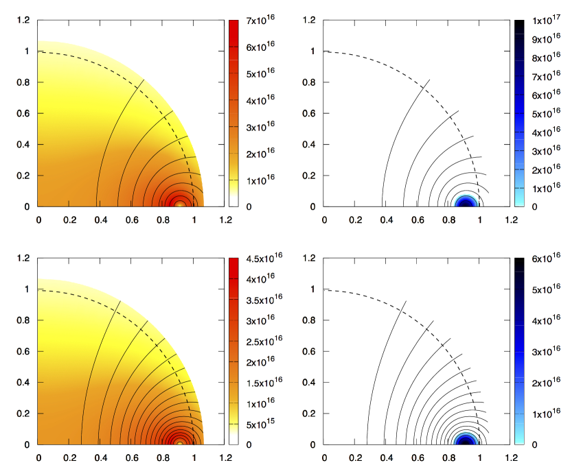
Figure 14: Two non-rotating models, slightly oblately distorted by the magnetic field. With the colourscales we plot the magnitude of the poloidal (left) and toroidal (right) field components, in units of gauss, together with the poloidal field lines. The dashed lines show the stellar surface. Top: $s_{b0}=0$, bottom: $s_{b0}=1.5$. These models feature around the strongest toroidal component, in terms of its contribution to the total magnetic energy, that our numerical method is able to find: $\mathcal{E}_{\rm mag}^{\rm tor}/\mathcal{E}_{\rm mag}=8.5\%$ for both. The magnetic-field structure of the hot model is virtually identical to the cold one, although the magnitudes of the field components are lower.

We now present some representative results for the magnetic field of a late proto-NS. Firstly, we look at a linked poloidal-toroidal magnetic field configuration; see Fig. 14. A very hot model, with $s_{b0}=1.5$, is compared with its zero-temperature counterpart. Although non-rotating, the two stars are slightly oblate by virtue of dominantly-poloidal magnetic fields (strong toroidal fields, by contrast, induce prolate distortions). In fact, all such self-consistent zero-temperature equilibria found to date feature a poloidal component that is energetically dominant, with the magnetic energy in the toroidal component $\mathcal{E}_{\rm mag}^{\rm tor}$ being only a small fraction of the total; one motivation for the work reported here was to see whether the same remained true for hot proto-NSs.

Fig. 14 demonstrates that the temperature of a NS plays essentially no role in determining the star’s magnetic-field structure, with the two models being indistinguishable. This strongly suggests that our simplified model for the thermal physics is perfectly adequate for this problem. Although we have chosen free functions in order to maximise the importance of the toroidal component (see section 5.2.1), only $8.5\%$ of the magnetic energy is stored in the toroidal component in both the hot and the cold models. The key difference is in the magnitude of the magnetic field, showing that a hot NS is more readily distorted by a magnetic field than its cold counterpart. We will explore this more in section 6.5.

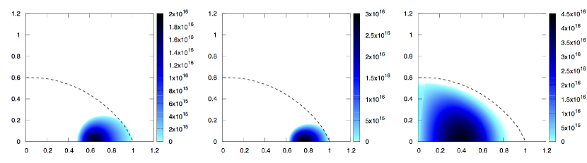
Figure 15: Toroidal field strength (colourscale) for three models with $s_{b0}=1.5$ and $\Omega=\Omega_{K}$, and all with an average internal field strength of $2\times 10^{16}$ G. The dashed line denotes the stellar surface. Left and middle: the toroidal component of a linked poloidal-toroidal field model with $\mathcal{E}_{\rm mag}^{\rm tor}/\mathcal{E}_{\rm mag}=5\%$ (left) and $10.7\%$ (middle). Right: a purely-toroidal field model.

Finally, in Fig. 15 we compare the distribution of toroidal field within two linked poloidal-toroidal models, and one purely-toroidal model, all rotating at Keplerian velocity. We consider three hot proto-NSs models, with $s_{b0}=1.5$; again, their cold counterparts are very similar in structure, but with different magnitudes. In the linked poloidal-toroidal models, we see that a slightly stronger toroidal component is possible compared with the almost-spherical non-rotating models of the previous figure: one model has $\mathcal{E}_{\rm mag}^{\rm tor}/\mathcal{E}_{\rm mag}=10.7\%$. We see an effect already known from cold models (Bucciantini et al., 2015; Armaza et al., 2015): as the maximum strength of the toroidal component is increased, the region it occupies decreases, leading to locally-intense toroidal fields whose contribution to the total magnetic energy is no larger than for locally-weaker counterparts.

6.5 Ellipticity

The magnetically-induced ellipticity, measuring the distortion from sphericity of a star’s mass distribution, is of interest, as a star with misaligned rotation and magnetic axes will emit continuous GWs at a magnitude proportional to this distortion (Bonazzola & Gourgoulhon, 1996). We find that it is somewhat easier to distort a hot star than a cold one. We constructed a number of magnetised and non-rotating models for a given $s_{b0}$, always finding that the results were in excellent agreement with the expected quadratic scaling $\epsilon=kB^{2}$. We then repeated the procedure for different values of $s_{b0}\leq 1.5$, finding that increases in $\epsilon$ were proportional to $s_{b0}^{2}$. Combining these results, we find a reasonable fit (deviating by less than 3% from all results) to the magnetically-induced ellipticity of a hot NS to be:

$$\epsilon=10^{-5}(3.0s_{b0}^{2}+8.3)\left({\frac{B_{\rm pole}}{10^{15}\textrm{ G}}}\right)^{2}=10^{-6}(2.3s_{b0}^{2}+6.5)\left({\frac{B_{\rm av}}{10^{15}\textrm{ G}}}\right)^{2}$$ (119)

for poloidal fields, and

$$\epsilon=-10^{-6}(2.1s_{b0}^{2}+6.9)\left({\frac{B_{\rm av}}{10^{15}\textrm{ G}}}\right)^{2}$$ (120)

for toroidal fields. In this latter case the ellipticity is negative, since the induced distortion is prolate. The results are only reported as a function of $B_{\rm av}$, since the toroidal magnetic-field strength drops to zero at the surface. The above formulae can readily be converted to a function of central temperature instead of entropy, using equation (118). Finally, results for mixed poloidal-toroidal models are not reported; the toroidal component only marginally reduces the oblateness (and therefore the ellipticity), since it occupies an insignificant low-density fraction of the stellar volume.

In the quadrupole formula for gravitational radiation, the ellipticity multiplies the moment of inertia of the star. The increase in $\epsilon$ we find could conceivably have been cancelled by a corresponding decrease in the moment of inertia, thus leading to no enhancement in the GW signal; however, upon checking this we found the moment of inertia varies very little with temperature (and, in fact, increases slightly).

6.6 Multipolar structure

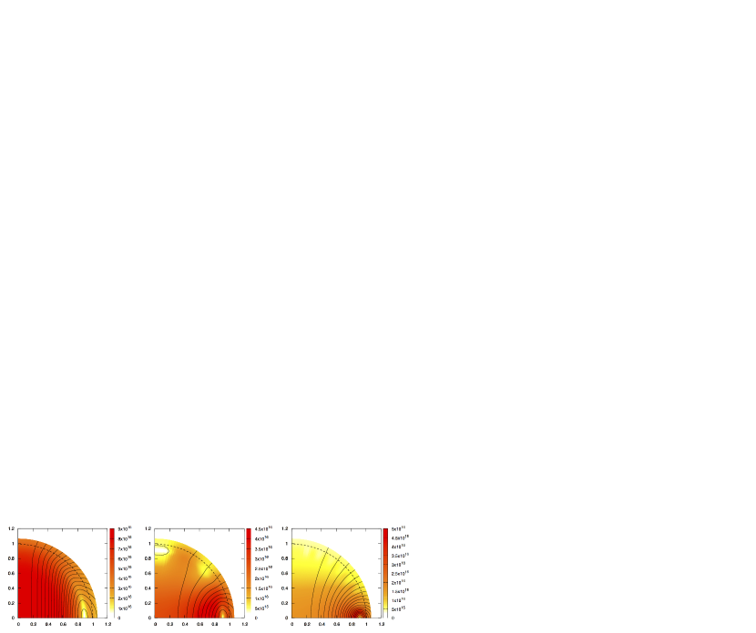
Figure 16: The effect of truncating equilibrium solutions at different multipoles. The magnitude (colourscale) and direction (lines) of the poloidal component of a linked poloidal-toroidal field are plotted for truncation at $l=1,4,16$ (left to right). All demonstrate unphysical artefacts from the truncation; convergence to a smooth solution is only achieved at $l=32$, shown in the bottom-left panel of Fig. 14.

Solution of the magnetic-equilibrium equations requires a multipolar decomposition of the exact vector equations into an infinite series of scalar equations in terms of different multipoles. Clearly one cannot in practice solve this infinite system, and must truncate the multipolar expansion at some value of the angular index. For semi-analytic models (e.g. Ciolfi et al. (2010)) it is only practicable to retain a few multipoles at best; in our numerical study we have the luxury of producing equilibria including the contributions of higher multipoles with little extra computational time.

In solving for a large-scale, global magnetic-field equilibrium, it is natural to expect the solution to be dominated by low-multipole contributions – but it is not clear how many multipoles should be retained for a faithful approximation to the exact infinite-multipole result. We check this in Fig. 16, for a linked poloidal-toroidal field whose toroidal component is very intense and localised in the outer equatorial region. We show only the poloidal component – strength and magnitude – since the toroidal component looks similar in each case. We find a major difference in the magnetic-field structures coming from truncating at low and high multipoles, and even between the $l=16$ and $32$ models; truncation for $l>32$, on the other hand, makes little difference. This is also seen in the ratio $\mathcal{E}_{\rm mag}^{\rm tor}/\mathcal{E}_{\rm mag}$, which is $2.4\%,3.4\%,8.2\%,8.5\%$ respectively for $l=1,4,16,32$.

We have undertaken similar comparisons for other cases. They are not plotted for reasons of brevity, but we find that high multipoles are similarly important in any magnetic-field model with significant stellar distortion (either from the magnetic field or rotation), but less so for almost-spherical poloidal-toroidal models without strong toroidal components. Only in this latter case (dominantly poloidal fields) is it safer to terminate at low multipoles.

In almost-spherical stars without extremely strong toroidal field components, the solution is seen to be dominated by the dipole component. However, for very intense toroidal components and/or significant stellar distortion, we see that a large number of multipoles must be summed before artefacts of the truncation cease to be visible.

7 Discussion

The primary motivation for undertaking this work was to study differences between the magnetic fields of young and mature NSs. They have turned out to be very similar, a result that raises more questions than it answers. In closing, it is therefore natural to discuss the implications of this result, and how realistic and general our results are.

7.1 Comparing cold and hot models

There were reasons to anticipate differences between cold and hot models. The strong thermal pressure – accounting for a substantial fraction of the star’s total pressure for our hottest models – represents a new piece of physics compared with a cold star. At the same time, we have not accounted for any kind of buoyancy force, even though they may play a role in a real proto-NS’s equilibrium; see section 3.2. The field is again governed by the Grad-Shafranov equation for barotropic fluids, whose solutions are only weakly affected by differences in the star’s pressure/density distribution. The core’s thermal pressure $P_{\rm th}\propto\rho^{5/3}$, which is not significantly different from the adiabatic index of $2-3$ for the zero-$T$ core pressure. We believe these two effects – the similar pressure distribution and the lack of buoyancy force – are the key reasons why the magnetic fields of hot equilibria are so similar to their cold counterparts. It also suggests that a relativistic version of our Newtonian equilibrium model – essentially amounting to changing the gravitational potential – would give similar results.

7.2 Relative strengths of poloidal and toroidal components

All of our new magnetic-field configurations for hot NSs are – like their cold predecessors – energetically dominated by the poloidal field component (the only exception being purely toroidal fields – but these are unstable and, having no exterior component, would not be directly observable). This is in conflict with a number of other pieces of work that rely on a NS’s magnetic field being dominated by its toroidal component. Typical supporting evidence invoked for dominantly-toroidal fields is the work of Braithwaite (2009) and Akgün et al. (2013), but we argue that the strong buoyancy forces required to support these equilibria may not exist in the proto-NS phase (and perhaps not at later stages either). To our knowledge the only barotropic NS model with a dominantly toroidal field is that presented in Ciolfi & Rezzolla (2013). With a careful choice of the magnetic functions $f(u)$ and $M(u)$ (see section 5.2.1), they were able to control the magnetic-field structure and produce a much wider range of poloidal- and toroidal-component strengths; see also Fujisawa & Eriguchi (2015) for a physical interpretation of this choice.

We have also experimented with a range of different choices for $f(u),M(u)$, including those of Ciolfi & Rezzolla (2013), but all of our resulting equilibria resemble those of Fig. 14 instead of ever having dominant toroidal components. There are two significant differences in our approach: firstly, our study involves numerical solution for self-consistent equilibria rather than an essentially analytic approach; secondly, that we retain a far higher number of multipoles in our solution (Ciolfi & Rezzolla (2013) only allowed for a dipole, $l=1$, field component). During our iterations we observe that even if we start with a larger region of toroidal field, as engineered by a careful choice of $f(u),M(u)$, this shrinks rapidly before the iterative method converges. How can we explain this disagreement? One possible scenario is that there is more than one branch of solutions to the Grad-Shafranov equation, and that our code ‘picks’ only a particular poloidal-dominated one. Another – and we believe more likely – possibility is that the results of Ciolfi & Rezzolla (2013) are only approximate equilibria, resulting from truncating at the dipole component and not considering the backreaction of the field – and that true self-consistent equilibrium models all resemble those we present in this work. We have already seen the dangers of truncating at low multipoles: in section 6.6, it was shown to cause serious errors in the resulting field configurations, including in the ratio $\mathcal{E}_{\rm mag}^{\rm tor}/\mathcal{E}_{\rm mag}$.

Further evidence for the universality of our poloidal-dominated equilibria is that at least two other independent numerical studies have also used the prescription of Ciolfi & Rezzolla (2013) without managing to obtain toroidal-dominated equilibria (Bucciantini et al. (2015); Armaza, private communication). The common feature of all three numerical codes seems to be the retention of high multipoles in the solutions; Fujisawa & Eriguchi (2015) also pointed out the likely importance of higher multipoles in their analysis of this problem. Finally, we note that non-linear evolutions of of an initially unstable magnetic field tend to show saturation to a state (albeit a dynamic one, not a strict equilibrium) with $\mathcal{E}_{\rm mag}^{\rm tor}/\mathcal{E}_{\rm mag}\;\raise 1.29167pt\hbox{$<$\kern-7.5pt\raise-4.73611pt\hbox{$\sim$}}\;25\%$ (Lasky et al., 2011; Ciolfi et al., 2011; Sur et al., 2020).

7.3 Stability and rearrangement of the field

We have argued that the magnetic field in a late proto-NS can be reasonably described as an equilibrium, and that such an equilibrium configuration appears to be poloidal-dominated in all cases. This has several implications. Firstly and most seriously, it has been argued that a stable magnetic equilibrium needs both poloidal and toroidal components, with at least comparable energies (Tayler, 1980) – which would imply there are no astrophysically relevant equilibria for proto-NSs at all. Qualitatively similar magnetic fields in zero-temperature models have been shown to be unstable (Lander & Jones, 2012), with the instability for poloidal-dominated fields developing in the region of closed field lines (where the toroidal component is also present). A glimmer of hope for the models presented here is that the temperature gradient may have a stablising effect; in addition, although the toroidal component is not energetically dominant, it can be locally comparable in strength with the poloidal one in the most unstable region of the star.

A second implication of our results is that a number of scenarios relying on a newborn NS having a strong toroidal field may be irrelevant, if no such field configuration exists. It is quite conceivable that differential rotation drives a strong amplification of the toroidal field component shortly after birth, but once this driving force ceases the field must rearrange into a state like our models. This suggests that at this early stage the magnetic field may shed a considerable amount of energy in its attempt to become an equilibrium state – an event likely to be powerful enough for detection. Furthermore, we have found that very rapidly-rotating stars can support stronger toroidal fields than non-rotating ones; this hints at another possible source of energy release from magnetic-field rearrangement on the star’s spindown timescale.

All our conclusions apply to relatively strong magnetic fields; see section 1.2. If instead the birth field is weak, so that the characteristic time for rearrangement is longer than the cooling timescale, we anticipate that it may avoid substantial rearrangement. Weaker NS magnetic fields could then have qualitatively different structures from stronger ones.

7.4 Lower break-up velocity

We find that a very hot proto-NS reaches break-up (Keplerian) velocity at a far lower rotational frequency than a cold model: by a factor of about a third. Our piecewise-polytropic treatment of the cold equation of state leads to a value of $\nu_{K}=960$ Hz for a $1.4\mathcal{M}_{\odot}$ cold star, in excellent agreement with the value $\nu_{K}=970$ Hz resulting from the approximate formula in Haensel et al. (2009) (within the range of accuracy of this approximation), but this drops below $\nu_{K}=700$ Hz for the hottest models, which can be explained by the significantly larger radii of these stars. Since the star is born hot, it is this latter, smaller value of $\nu_{K}$ that sets the effective limiting rotation rate in the star’s early life. Note that for all plausible field strengths ($B\;\raise 1.29167pt\hbox{$<$\kern-7.5pt\raise-4.73611pt\hbox{$\sim$}}\;10^{17}$ G), the magnetic field has no effect on the value of $\nu_{K}$ (Lander & Jones, 2009). This low value of $\nu_{K}$ may make it more difficult to realise various interesting scenarios: gravitational waves from unstable $r$- or $f$-modes in rapidly-rotating newborn NSs, or millisecond magnetars and their associated electromagnetic/gravitational radiation. Our limiting rotation rate is however not relevant for explaining the puzzle of rotation rates of old, recycled NSs having an upper limit well below $\nu_{K}$, since for this scenario the cold value is relevant.

7.5 The future of the proto-NS’s magnetic field

The majority of observed NSs have strong magnetic fields with large-scale structure. They have no obvious mechanism for regeneration of magnetic flux, indicating that the field remaining at the end of the proto-NS phase is not substantially dissipated over thousands of years. We have argued, however, that instabilities may plague our models – and such instabilities involve widespread disruption to the magnetic field and turbulent fluid motions, which are likely to cause a major loss of magnetic energy.

The resolution to this contradiction could be an additional piece of proto-NS physics – for example, if differential rotation persists into this late stage and allows for a stronger toroidal field than in our models – or the advent of a new stabilising mechanism as the star cools. A day into its life, with a temperature not much above $10^{9}$ K (Gnedin et al., 2001), a NS will have started developing two such candidate mechanisms: a modest but growing region of superconducting protons in its core, and solidification of its envelope into a crust, starting from the boundary with the core and slowly moving outwards. Both may inhibit magnetic instabilities: the former by changing the local structure and dynamics of the field, and the latter by providing an elastic force to resist unstable motion.

Two factors may assist the crust in stabilising the stellar magnetic field. Firstly, although the toroidal-field component might not itself stabilise the poloidal-dominated field, it can help indirectly by pushing the unstable closed-field-line region outwards into the crust (see section 6.4). Secondly, a strong magnetic field induces the formation of an extended inner crust region (Fang et al., 2017), which could be as much as $\sim 1$ km in a magnetar, thus increasing the likelihood of the closed-field-line region coinciding with the crust (Sengo et al., 2020).

7.6 Outlook

The study of NS magnetic fields has reached a juncture, where quantitative models tend to include only very simple physics, and where consideration of more realistic physics is often speculative and qualitative. Quantitative studies of the birth phase of NS magnetic fields are likely to be crucial to improving this situation: the dynamo processes generating magnetic flux straight after birth, the immediate post-dynamo phase in which the field should presumably relax into an equilibrium, and the later formation of a solid crust and superconducting regions in the core. We have tried, in this work, to take a first step in that direction.

Data availability

The specific data underlying this article, and additional data for other stellar models, will be made available upon reasonable request.

References

- Akgün et al. (2013) Akgün T., Reisenegger A., Mastrano A., Marchant P., 2013, MNRAS, 433, 2445
- Armaza et al. (2015) Armaza C., Reisenegger A., Valdivia J. A., 2015, ApJ, 802, 121
- Bocquet et al. (1995) Bocquet M., Bonazzola S., Gourgoulhon E., Novak J., 1995, A&A, 301, 757
- Bonazzola & Gourgoulhon (1996) Bonazzola S., Gourgoulhon E., 1996, A&A, 312, 675
- Braithwaite (2009) Braithwaite J., 2009, MNRAS, 397, 763
- Braithwaite & Cantiello (2013) Braithwaite J., Cantiello M., 2013, MNRAS, 428, 2789
- Bucciantini et al. (2015) Bucciantini N., Pili A. G., Del Zanna L., 2015, MNRAS, 447, 3278
- Burrows & Lattimer (1986) Burrows A., Lattimer J. M., 1986, ApJ, 307, 178
- Camelio et al. (2017) Camelio G., Lovato A., Gualtieri L., Benhar O., Pons J. A., Ferrari V., 2017, Phys. Rev. D, 96, 043015
- Camelio et al. (2019) Camelio G., Dietrich T., Marques M., Rosswog S., 2019, Phys. Rev. D, 100, 123001
- Cameron (1959) Cameron A. G., 1959, ApJ, 130, 884
- Castillo et al. (2020) Castillo F., Reisenegger A., Valdivia J. A., 2020, MNRAS, 498, 3000
- Ciolfi & Rezzolla (2013) Ciolfi R., Rezzolla L., 2013, MNRAS, 435, L43
- Ciolfi et al. (2010) Ciolfi R., Ferrari V., Gualtieri L., 2010, MNRAS, 406, 2540
- Ciolfi et al. (2011) Ciolfi R., Lander S. K., Manca G. M., Rezzolla L., 2011, ApJ, 736, L6
- Colgate & White (1966) Colgate S. A., White R. H., 1966, ApJ, 143, 626
- Douchin & Haensel (2001) Douchin F., Haensel P., 2001, A&A, 380, 151
- Fang et al. (2017) Fang J., Pais H., Pratapsi S., Avancini S., Li J., Providência C., 2017, Phys. Rev. C, 95, 045802
- Fujisawa & Eriguchi (2015) Fujisawa K., Eriguchi Y., 2015, PASJ, 67, 53
- Glampedakis & Lasky (2016) Glampedakis K., Lasky P. D., 2016, MNRAS, 463, 2542
- Glampedakis et al. (2011) Glampedakis K., Andersson N., Samuelsson L., 2011, MNRAS, 410, 805
- Glampedakis et al. (2014) Glampedakis K., Lander S. K., Andersson N., 2014, MNRAS, 437, 2
- Gnedin et al. (2001) Gnedin O. Y., Yakovlev D. G., Potekhin A. Y., 2001, MNRAS, 324, 725
- Goussard et al. (1997) Goussard J. O., Haensel P., Zdunik J. L., 1997, A&A, 321, 822
- Grad & Rubin (1958) Grad H., Rubin H., 1958, in 2nd United Nations Int. Conf. on Peaceful Uses of Atomic Energy, Geneva. p. 190
- Gusakov et al. (2017) Gusakov M. E., Kantor E. M., Ofengeim D. D., 2017, Phys. Rev. D, 96, 103012
- Hachisu (1986) Hachisu I., 1986, ApJS, 61, 479
- Haensel & Pichon (1994) Haensel P., Pichon B., 1994, A&A, 283, 313
- Haensel et al. (2007) Haensel P., Potekhin A. Y., Yakovlev D. G., 2007, Neutron Stars 1 : Equation of State and Structure. Vol. 326
- Haensel et al. (2009) Haensel P., Zdunik J. L., Bejger M., Lattimer J. M., 2009, A&A, 502, 605
- Jackson et al. (2005) Jackson S., MacGregor K. B., Skumanich A., 2005, ApJS, 156, 245
- Janka et al. (2007) Janka H. T., Langanke K., Marek A., Martínez-Pinedo G., Müller B., 2007, Phys. Rep., 442, 38
- Kiuchi & Kotake (2008) Kiuchi K., Kotake K., 2008, MNRAS, 385, 1327
- Kiuchi et al. (2009) Kiuchi K., Kotake K., Yoshida S., 2009, ApJ, 698, 541
- Landau & Lifshitz (1993) Landau L. D., Lifshitz E. M., 1993, Statistical Physics, Part 1. Oxford: Pergamon Press
- Lander (2014) Lander S. K., 2014, MNRAS, 437, 424
- Lander & Jones (2009) Lander S. K., Jones D. I., 2009, MNRAS, 395, 2162
- Lander & Jones (2011) Lander S. K., Jones D. I., 2011, MNRAS, 412, 1730
- Lander & Jones (2012) Lander S. K., Jones D. I., 2012, MNRAS, 424, 482
- Lander et al. (2010) Lander S. K., Jones D. I., Passamonti A., 2010, MNRAS, 405, 318
- Lander et al. (2012) Lander S. K., Andersson N., Glampedakis K., 2012, MNRAS, 419, 732
- Lasky et al. (2011) Lasky P. D., Zink B., Kokkotas K. D., Glampedakis K., 2011, ApJ, 735, L20
- Lin & Ogilvie (2018) Lin Y., Ogilvie G. I., 2018, MNRAS, 474, 1644
- Mastrano et al. (2011) Mastrano A., Melatos A., Reisenegger A., Akgün T., 2011, MNRAS, 417, 2288
- Ofengeim & Gusakov (2018) Ofengeim D. D., Gusakov M. E., 2018, Phys. Rev. D, 98, 043007
- Pili et al. (2015) Pili A. G., Bucciantini N., Del Zanna L., 2015, MNRAS, 447, 2821
- Pons & Viganò (2019) Pons J. A., Viganò D., 2019, Living Reviews in Computational Astrophysics, 5, 3
- Pons et al. (1999) Pons J. A., Reddy S., Prakash M., Lattimer J. M., Miralles J. A., 1999, ApJ, 513, 780
- Potekhin & Chabrier (2000) Potekhin A. Y., Chabrier G., 2000, Phys. Rev. E, 62, 8554
- Prakash et al. (1997) Prakash M., Bombaci I., Prakash M., Ellis P. J., Lattimer J. M., Knorren R., 1997, Phys. Rep., 280, 1
- Read et al. (2009) Read J. S., Lackey B. D., Owen B. J., Friedman J. L., 2009, Phys. Rev. D, 79, 124032
- Reisenegger (2009) Reisenegger A., 2009, A&A, 499, 557
- Sengo et al. (2020) Sengo I., Pais H., Franzon B., Providência C., 2020, arXiv e-prints, p. arXiv:2006.07248
- Shafranov (1958) Shafranov V. D., 1958, Soviet Journal of Experimental and Theoretical Physics, 6, 545
- Spruit (2009) Spruit H. C., 2009, in Strassmeier K. G., Kosovichev A. G., Beckman J. E., eds, Vol. 259, Cosmic Magnetic Fields: From Planets, to Stars and Galaxies. pp 61–74, doi:10.1017/S1743921309030075
- Sur et al. (2020) Sur A., Haskell B., Kuhn E., 2020, MNRAS, 495, 1360
- Tayler (1980) Tayler R. J., 1980, MNRAS, 191, 151
- Thompson & Duncan (1993) Thompson C., Duncan R. C., 1993, ApJ, 408, 194
- Tomimura & Eriguchi (2005) Tomimura Y., Eriguchi Y., 2005, MNRAS, 359, 1117
- Uryū et al. (2019) Uryū K., Yoshida S., Gourgoulhon E., Markakis C., Fujisawa K., Tsokaros A., Taniguchi K., Eriguchi Y., 2019, Phys. Rev. D, 100, 123019
- Villain et al. (2005) Villain L., Bonazzola S., Haensel P., 2005, Phys. Rev. D, 71, 083001
- Woosley et al. (2002) Woosley S. E., Heger A., Weaver T. A., 2002, Reviews of Modern Physics, 74, 1015