Chiral Four-Wave-Mixing signals with circularly-polarized X-ray pulses

Abstract

Chiral four-wave-mixing signals are calculated using the irreducible tensor formalism. Different polarization and crossing angle configurations allow to single out the magnetic dipole and the electric quadrupole interactions. Other configurations can reveal that the chiral interaction occurs at a given step within the nonlinear interaction pathways contributing to the signal. Applications are made to the study of valence excitations of S-ibuprofen by chiral Stimulated X-ray Raman signals at the Carbon K-edge and by chiral visible 2D Electronic Spectroscopy.

1 Introduction

Chirality is the notable property of molecules lacking mirror symmetry. This simple geometrical constraint has profound implications on fundamental science¹, biological activity² and drug synthesis³. Numerous techniques have been implemented to detect and discriminate opposite enantiomers with high precision. These include now routine spectroscopies such as Circular Dichroism (CD)^{4, 5} or Optical Activity (OA)⁶ as well as more advanced ones like Raman Optical Activity (ROA)⁶ or Photoelectron CD (PECD)⁷. Differences of observables involving various polarization configurations permit to cancel the achiral contributions and single out the chiral ones. Most chiral-sensitive spectroscopies suffer from an unfavorable signal-to-noise ratio since the ratio of chiral to achiral signals is usually of the order of a percent or less (the ratio of molecular size to the optical wavelength).
The application of third-order nonlinear spectroscopies to measure chiral signals has gained experimental and theoretical interest over the past decades^{8, 9, 10, 11}. Belkin and Shen¹² have focused on second-order $\chi^{(2)}$ signals that vanish altogether in an achiral isotropic sample. Most spectroscopic measurements of matter chirality are carried out on randomly oriented samples. In non isotropic samples, important artefacts cover the CD signals such as linear dichroism or birefringence and must be dealt with¹³. Here, we focus on molecules in the liquid or gas phase where the molecular response must be rotationally averaged. Rotational averagings of cartesian¹⁴ and spherical¹⁵ tensors are well established. We use the irreducible tensor formalism^{15, 16} to carry out the rotational averages. This is very convenient since only the $J=0$ tensor components do not vanish upon averaging.

In this study, we demonstrate that chiral nonlinear signals offer a way to control which chiral pathways contribute to the final signals by using various polarization and pulse geometry configurations. In particular, we show that signals involving the chiral interaction at a given step along the interaction pathways can be extracted. We have calculated chiral signals that only depend only on the magnetic dipole or on the electric quadrupole interactions. These allow to assign explicitly the multipolar nature of a given transition. This is of importance to describe near field chiral interactions^{17, 18} and for the emergence of X-ray chiral sensitive signals where the relative magnitudes of electric quadrupole and magnetic dipole may be very different than at the visible and infrared frequency regimes¹⁹.

We focus on chiral four-wave-mixing (4WM) signals. Several polarization schemes can single out chiral contributions by highlighting different types of interactions. In section 2, we first present 4WM spectroscopies in general terms using the multipolar interaction Hamiltonian. We compute all possible combinations of chiral-sensitive 4WM techniques and discuss the averaging of signals using the irreducible tensor representation of the 4WM response tensors. Finally, in section 3, we apply this formalism to study valence excitations in the drug S-ibuprofen by Stimulated X-ray Raman Spectroscopy (SXRS) and 2D Electronic Spectroscopy (2DES).

2 Multipolar representation of four-wave-mixing signals

We start with the multipolar radiation-matter coupling Hamiltonian that includes the electric and magnetic dipoles and the electric quadrupole:

$$H_{\text{int}}(t)=-\bm{\mu}\cdot\mathbb{E}(t)-\bm{m}\cdot\mathbb{B}(t)-\bm{q}\cdot\nabla\mathbb{E}(t)$$ (1)

We consider 3 four wave mixing techniques denoted $\mathbb{k}_{I},\mathbb{k}_{II}$ and $\mathbb{k}_{III}$ according to their phase matching direction

$$\mathbb{k}_{I} = -\mathbb{k}_{1}+\mathbb{k}_{2}+\mathbb{k}_{3}$$ (2)

$$\mathbb{k}_{II} = +\mathbb{k}_{1}-\mathbb{k}_{2}+\mathbb{k}_{3}$$ (3)

$$\mathbb{k}_{III} = +\mathbb{k}_{1}+\mathbb{k}_{2}-\mathbb{k}_{3}$$ (4)

$\bm{k}_{1}$, $\bm{k}_{2}$ and $\bm{k}_{3}$ are the wavevectors of the time-ordered incoming pulses. We use the vectors $(u_{1},u_{2},u_{3})=(-1,1,1),\ (1,-1,1),\ (1,1,-1)$ to represent the $\mathbb{k}_{I},\mathbb{k}_{II}$ and $\mathbb{k}_{III}$ techniques respectively. In a three level system, the $\mathbb{k}_{I}$ and $\mathbb{k}_{II}$ techniques contain three pathways (excitated state emission ESE, ground state bleaching GSB and excited state absorption ESA) while $\mathbb{k}_{III}$ has only two ESA pathways. These pathways indicate whether the molecule is back in the ground state after the first two interactions (GSB) or in an excited state (ESE and ESA)²⁰.

The heterodyne-detected four-wave-mixing signal generally contains chiral and nonchiral components

$$S_{\text{het}}(\Gamma)=S_{\text{achir}}(\Gamma)+S_{\text{chir}}(\Gamma)$$ (5)

where $\Gamma$ represents collectively the set of parameters that control the multidimensional signal (typically central frequencies, polarizations, bandwidths) as well as the wavevector configuration ($\mathbb{k}_{I},\mathbb{k}_{II}$ or $\mathbb{k}_{III}$). The achiral contribution $S_{\text{achir}}$ is given by the purely electric dipole contribution⁹:

$$S_{\text{achir}}(\Gamma)=-\frac{2}{\hbar}\Im\int dtdt_{3}dt_{2}dt_{1}\mathbb{\mathbb{missing}}R_{\mu\mu\mu\mu}(t_{3},t_{2},t_{1})\bullet(\mathbb{E}_{s}(t)\otimes\mathbb{E}_{3}(t-t_{3})\otimes\mathbb{E}_{2}(t-t_{3}-t_{2})\\ \otimes\mathbb{E}_{1}(t-t_{3}-t_{2}-t_{1}))$$ (6)

with

$$\mathbb{R}_{\mu\mu\mu\mu}(t_{3},t_{2},t_{1})=\Big{(}-\frac{i}{\hbar}\Big{)}^{3}\langle\bm{\mu}_{\text{left}}\mathcal{G}(t_{3})\bm{\mu}_{-}\mathcal{G}(t_{2})\bm{\mu}_{-}\mathcal{G}(t_{1})\bm{\mu}_{-}\rangle$$ (7)

$\mathbb{R}_{\mu\mu\mu\mu}$ is a sum of pathways with four electric dipoles. At the lowest multipolar order, the chiral contribution $S_{\text{chiral}}$ contains either one magnetic dipole or one electric quadrupole and is given by

$$S_{\text{chiral}}(\Gamma)=-\frac{2}{\hbar}\Im\int dtdt_{3}dt_{2}dt_{1}$$

$$(\bm{R}_{m\mu\mu\mu}\bullet(\mathbb{B}_{s}\otimes\mathbb{E}_{3}\otimes\mathbb{E}_{2}\otimes\mathbb{E}_{1})+\bm{R}_{q\mu\mu\mu}\bullet(\nabla\mathbb{E}_{s}\otimes\mathbb{E}_{3}\otimes\mathbb{E}_{2}\otimes\mathbb{E}_{1})$$

$$+\bm{R}_{\mu m\mu\mu}\bullet(\mathbb{E}_{s}\otimes\mathbb{B}_{3}\otimes\mathbb{E}_{2}\otimes\mathbb{E}_{1})+\bm{R}_{\mu q\mu\mu}\bullet(\mathbb{E}_{s}\otimes\nabla\mathbb{E}_{3}\otimes\mathbb{E}_{2}\otimes\mathbb{E}_{1})$$

$$+\bm{R}_{\mu\mu m\mu}\bullet(\mathbb{E}_{s}\otimes\mathbb{E}_{3}\otimes\mathbb{B}_{2}\otimes\mathbb{E}_{1})+\bm{R}_{\mu\mu q\mu}\bullet(\mathbb{E}_{s}\otimes\mathbb{E}_{3}\otimes\nabla\mathbb{E}_{2}\otimes\mathbb{E}_{1})$$

$$+\bm{R}_{\mu\mu\mu m}\bullet(\mathbb{E}_{s}\otimes\mathbb{E}_{3}\otimes\mathbb{E}_{2}\otimes\mathbb{B}_{1})+\bm{R}_{\mu\mu\mu q}\bullet(\mathbb{E}_{s}\otimes\mathbb{E}_{3}\otimes\mathbb{E}_{2}\otimes\nabla\mathbb{E}_{1}))$$ (8)

where we have omitted the time variable for conciseness. The multipolar matter correlation functions are given by:

$$\mathbb{R}_{m\mu\mu\mu}(t_{3},t_{2},t_{1}) = \Big{(}-\frac{i}{\hbar}\Big{)}^{3}\langle\bm{m}_{\text{left}}\mathcal{G}(t_{3})\bm{\mu}_{-}\mathcal{G}(t_{2})\bm{\mu}_{-}\mathcal{G}(t_{1})\bm{\mu}_{-}\rangle$$ (9)

$$\mathbb{R}_{q\mu\mu\mu}(t_{3},t_{2},t_{1}) = \Big{(}-\frac{i}{\hbar}\Big{)}^{3}\langle\bm{q}_{\text{left}}\mathcal{G}(t_{3})\bm{\mu}_{-}\mathcal{G}(t_{2})\bm{\mu}_{-}\mathcal{G}(t_{1})\bm{\mu}_{-}\rangle$$ (10)

The four magnetic dipole and the four electric quadrupole response functions in Eq. 8 are obtained by permuting the position of the $\bm{m}$ or $\bm{q}$ within each interaction pathway. The subscripts $(\text{left})$ and $(-)$ indicates Liouville space superoperators²¹. The Liouville space superoperators are defined by their action on Hilbert space operators as $\mathcal{O}_{\text{left}}\mathcal{A}\equiv\mathcal{O}\mathcal{A}$ and $\mathcal{O}_{\text{right}}\mathcal{A}\equiv\mathcal{A}\mathcal{O}$. We further define their linear combinations $\mathcal{O}_{\pm}$ which correspond to commutators and anticommutators in Hilbert space as $\mathcal{O}_{\pm}\mathcal{A}\equiv\mathcal{O}\mathcal{A}\pm\mathcal{A}\mathcal{O}.$ Such operators allow to keep track of interactions on the ket or bra side of the density matrix.

Assuming a slowly varying electric field envelope, we can express the magnetic fields and the electric field gradients as:

$$\bm{E}_{i}(t) = \mathcal{E}_{i}(t)\ \bm{\epsilon}_{i}$$ (11)

$$\bm{B}_{i}(t) = \mathcal{E}_{i}(t)\ \frac{1}{c}u_{i}\bm{\hat{k}}_{i}\wedge\bm{\epsilon}_{i}$$ (12)

$$\bm{\nabla}E_{i}(t) = \mathcal{E}_{i}(t)\ iu_{i}\frac{\omega_{i}}{c}\bm{\hat{k}}_{i}\otimes\bm{\epsilon}_{i}$$ (13)

where $\bm{\epsilon}_{i}$ is the polarization unit vector of the $i$th pulse electric field.

The chiral contributions to 4WM are defined for rotationally-averaged samples and will be calculated using the irreducible tensor algebra¹⁶. In this formalism, cartesian tensors are expanded in irreducible tensors, i.e. tensors transforming according to the irreducible representations of the rotation group SO(3): $T=\sum_{\tau J}\ {}_{\tau}T^{J}$ where $\tau$ is the seniority index which depends on the coupling scheme of matter quantities constituting the response tensor. This formalism is a generalization of the decomposition of a matrix into its trace, an anti-symmetric part and a traceless symmetric part. For 4WM signals, we apply it to rank 4 and 5 cartesian tensors. Irreducible tensors up to irreducible rank $J=5$ appear in the decomposition of the matter and field tensors. The strength of the formalism resides in that only the isotropic $J=0$ tensors contributes to the rotationally averaged signals and thus need to be calculated.^{16, 22} The signal is given by an irreducible tensor product of the matter response function $\bm{R}$ and the field tensor $\bm{F}$:

$$\bm{R}\cdot\bm{F}=\sum_{\tau J}\sum_{M=-J}^{J}(-1)^{M}\ _{\tau}R^{JM}\ _{\tau}F^{J-M}$$ (14)

The field tensor $F$ is kept general here and in practice will be described by a direct product of four field functions $\bm{E},\bm{B}$ or $\nabla\bm{E}$. For example, the response tensor $R_{m\mu\mu\mu}$ and $R_{q\mu\mu\mu}$ are contracted with $\bm{B}\otimes\bm{E}\otimes\bm{E}\otimes\bm{E}$ and $\nabla\bm{E}\otimes\bm{E}\otimes\bm{E}\otimes\bm{E}$ respectively.

The rotationally-averaged contraction between matter and field response tensor is obtained by retaining only the $J=0$ terms:

$$(\bm{R}\cdot\bm{F})_{\text{av}}=\sum_{\tau}\ {}_{\tau}R_{\text{dip-E}}^{J=0}\ {}_{\tau}F_{\text{elec}}^{J=0}+\ _{\tau}R_{\text{dip-M}}^{J=0}\ {}_{\tau}F_{\text{mag}}^{J=0}+\ _{\tau}R_{\text{quad-E}}^{J=0}\ {}_{\tau}G_{\text{quad}}^{J=0}$$ (15)

where the general expression for the matter and the field tensors are given in Appendix A and in supplementary materials, section 1. The field tensors ${}_{\tau}F_{\text{elec}}^{J=0}$ and ${}_{\tau}F_{\text{mag}}^{J=0}$ are calculated from the rank 4 cartesian tensors while the ${}_{\tau}G_{\text{quad}}^{J=0}$ is calculated from the rank 5 tensors involving $\nabla\bm{E}$.

As is done in circular dichroism (CD) or Raman optical activity (ROA), combinations of various polarization configurations can lead to the cancellation of the achiral electric dipole contribution and provides a measure of the chiral response function. The electric dipole invariant tensor components have even parity while the magnetic dipole and electric quadrupole ones have an odd parity.

Unlike the linear CD, nonlinear 4WM signals offer multiple possible cancellation scenarios of the achiral components which can be combined in order to enhance desired features of the signal. There are four possible chiral polarization configurations (denoted $\alpha,\beta,\gamma$ and $\delta$) for each of the phase matching directions ($\mathbb{k}_{i}=\mathbb{k}_{I}$, $\mathbb{k}_{II}$ and $\mathbb{k}_{III}$), leading to 12 possible schemes, see Eqs. 16-19. Each of them further depends on the crossing angles of the incoming pulses. There are thus many ways to access the chiral response functions with various degrees of control.

The four polarization schemes are given by

$$S_{\text{chir}}(\alpha,\bm{k}_{i}) = S_{\text{het}}(L,L,L,L)-S_{\text{het}}(R,R,R,R)$$ (16)

$$S_{\text{chir}}(\beta,\bm{k}_{i}) = S_{\text{het}}(L,R,L,R)-S_{\text{het}}(R,L,R,L)$$ (17)

$$S_{\text{chir}}(\gamma,\bm{k}_{i}) = S_{\text{het}}(L,L,R,R)-S_{\text{het}}(R,R,L,L)$$ (18)

$$S_{\text{chir}}(\delta,\bm{k}_{i}) = S_{\text{het}}(L,R,R,L)-S_{\text{het}}(R,L,L,R)$$ (19)

where the arguments of $S_{\text{het}}(e_{s},e_{3},e_{2},e_{1})$ indicate the polarization of pulses $\bm{E}_{s}$, $\bm{E}_{3}$, $\bm{E}_{2}$ and $\bm{E}_{1}$ and $\mathbb{k}_{i}=\mathbb{k}_{I},\mathbb{k}_{II}$ or $\mathbb{k}_{III}$.

We shall show that it is possible to experimentally select signals occurring solely through magnetic dipole or through electric quadrupole interactions. It is also possible to identify signals whereby the chiral interaction occurs at a given step in the interaction pathways.

3 Resonant chiral SXRS and 2DES signals in S-ibuprofen

3.1 Ibuprofen quantum chemistry

The valence electronic excited states of S-ibuprofen (Fig. 1a) were computed using multi configurational self-consistent field (MCSCF) calculations at the cc-pVDZ/CASSCF(8/7) level of theory using the MOLPRO package²³.

The core-excited states were calculated at the cc-pVDZ/RASSCF(9/8) level by moving one by one the 1s carbon orbitals into the active space and freezing it to a single occupancy. The second order Douglas-Kroll-Hess Hamiltonian was used to account for relativistic corrections²⁴. The valence and core excited states stick spectra compared with experiment^{25, 26} are displayed in Fig. 1 b) and c).

Figure 1: a) Molecular structure of S-ibuprofen. b) Experimental UV absorption from Moore et al.²⁵ (blue) and stick spectrum calculated at the cc-pVDZ/CASSCF(8/7) level. c) Experimental X-ray absorption ²⁶ (blue) and stick spectrum at the cc-pVDZ/CASSCF(8/7). The dashed red curve is computed from the stick spectrum by convoluting with Lorentzian lineshapes and a step function accounting for ionization contributions.

3.2 Chiral Stimulated X-ray Raman Spectroscopy

We now employ the polarization configurations developed earlier to compute the chiral Stimulated X-ray Raman Spectra (cSXRS), at the carbon K edge, as sketched in Fig. 2. This pump-probe technique involves two ultrashort X-ray pulses, Fig. 2a, whose variation with their delay carries information on the valence excitation manifold. Each X-ray pulse induces a stimulated Raman process in the molecule (Fig. 2b) and its broad bandwidth allows to pump or probe many valence excited states in a single shot with high temporal resolution. The core resonance allows to control which atoms are excited and probed, and the signal thus carries information about the valence excitations in the vicinity of the selected core.

Figure 2: a) Pulse configuration for SXRS. b) Jablonski energy levels contributing to the SXRS signal. $g$ is the ground state, $e$ is the valence excited state manifold and $c$ the core excited state one. c) Ladder diagrams for SXRS. To account for the lack of time ordering of the interactions with the first pulse, each of these diagrams contributes twice to the signal. Upon Fourier transforming over the time delay, only the left diagram contributes to positive frequencies.

The signal can be read off the loop diagrams displayed in Fig. 2c and reads

$$S_{\text{SXRS}}(T)=-\frac{2}{\hbar}\Im(\frac{i}{\hbar})^{3}\int dtds_{3}ds_{2}ds_{1}\bm{E}_{2}^{*}(t)\bm{E}_{2}(t-s_{3})\Big{(}\\ \langle\Psi(t_{0})|G^{\dagger}(t)\bm{\mu}G(s_{3})\bm{\mu}^{\dagger}G(s_{2})\bm{\mu}G(s_{1})\bm{\mu}^{\dagger}G(t-s_{3}-s_{2}-s_{1})|\Psi(t_{0})\rangle\bm{E}_{1}^{*}(t-s_{3}-s_{2})E_{1}(t-s_{3}-s_{2}-s_{1})\\ +\langle\Psi(t_{0})|G^{\dagger}(t-s_{2}-s_{1})\bm{\mu}G^{\dagger}(s_{1})\bm{\mu}^{\dagger}G^{\dagger}(s_{2})\bm{\mu}G(s_{3})\bm{\mu}^{\dagger}G(t-s_{3})|\Psi(t_{0})\rangle\bm{E}_{1}(t-s_{2})\bm{E}_{1}(t-s_{2}-s_{1})\Big{)}$$ (20)

By expanding this expression in molecular eigenstates, transforming the fields into the frequency domain and taking the Fourier transform over $T$, we obtain the following expressions for the electric dipole contribution to the signal:

$$S_{\text{SXRS}}(\Omega)=|E_{2}|^{2}|E_{1}|^{2}\frac{2}{\hbar^{4}}\Im\sum_{ecc^{\prime}}\bm{\mu}_{gc^{\prime}}\bm{\mu}^{\dagger}_{c^{\prime}e}\bm{\mu}_{ec}\bm{\mu}^{\dagger}_{cg}\frac{I_{2,c^{\prime}g}(\Omega)I_{1,cg}(\Omega)}{\Omega-\omega_{eg}+i\epsilon}$$ (21)

$$I_{2,c^{\prime}g}(\Omega)=\frac{e^{-\Omega^{2}/4\sigma_{2}^{2}}}{2\sigma_{2}^{2}}e^{-z_{2}^{2}}(i+\text{erfi}(z_{2}))\ \ \ \ \ \ \ \text{with}\ \ \ \ \ \ \ z_{2}=-\frac{1}{\sigma_{2}}(\omega_{2}+\Omega/2-\omega_{c^{\prime}g}+i\epsilon)\\ I_{1,cg}(\Omega)=\frac{e^{-\Omega^{2}/4\sigma_{2}^{2}}}{2\sigma_{1}^{2}}e^{-z_{1}^{2}}(i+\text{erfi}(z_{1}))\ \ \ \ \ \ \ \text{with}\ \ \ \ \ \ \ z_{1}=-\frac{1}{\sigma_{1}}(\omega_{1}+\Omega/2-\omega_{cg}+i\epsilon)$$ (22)

where $I_{1,cg}(\Omega)$ and $I_{2,c^{\prime}g}(\Omega))$ are the lineshape functions associated with the first and second X-ray pulses respectively.

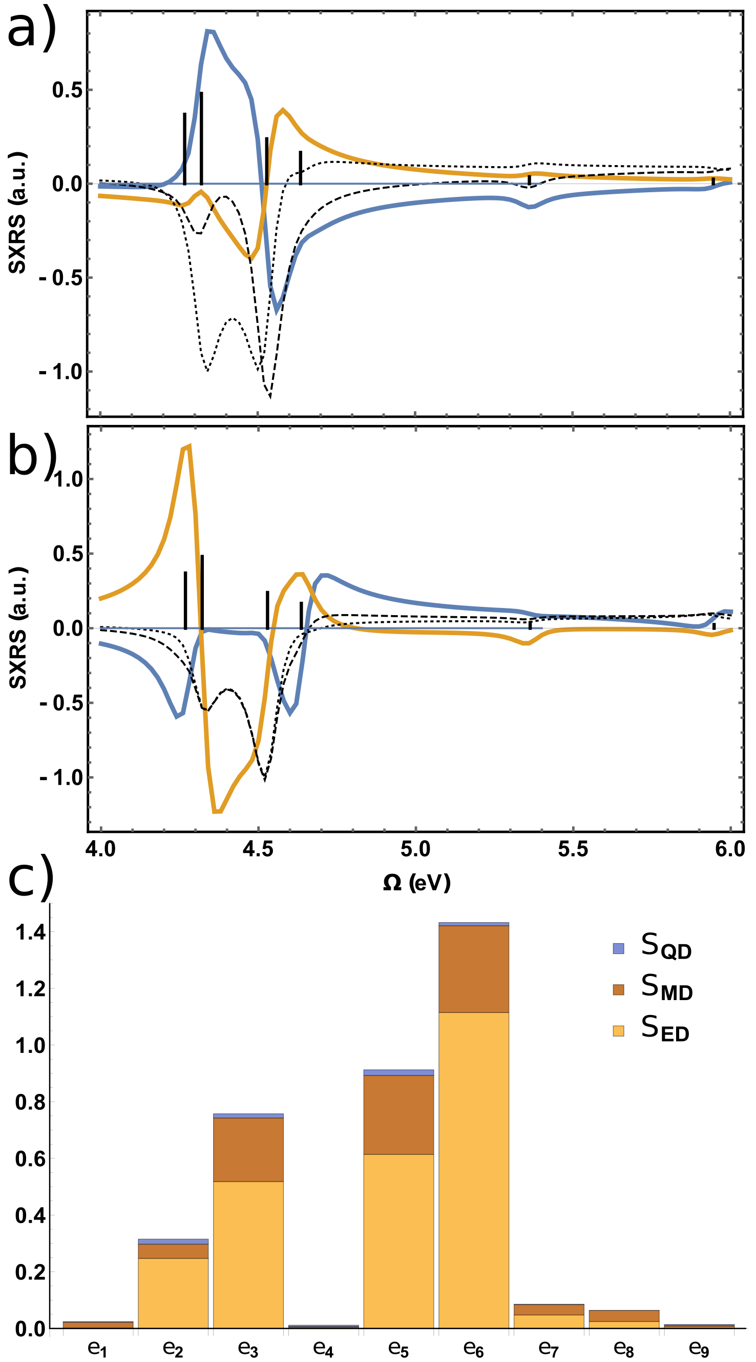
Figure 3: a) cSXRS($\Omega$,$\alpha$) signal of ibuprofen. Blue: both X-ray pulses are centred at the chiral carbon 1s core-excitation transition energy (283.8 eV). Orange: the first pulse is tuned at the chiral carbon 1s core transition and the second pulse is tuned at the carbon in the propyl group (286.6 eV). The dashed and dotted curves are the total SXRS signals with LL and RR polarization configurations respectively. The total SXRS signals are normalized and the cSXRS are multiplied by 5. In b) cSXRS($\Omega$,$\beta$) signal with similar pulse central frequencies. The dashed and dotted curves are the total SXRS signals with LR and RL polarization configurations respectively. c) Relative multipolar contributions from each state to the total SXRS signals.

The other contributions are obtained by replacing one of the electric dipoles in Eq. 21 with a magnetic dipole or with an electric quadrupole, following Eq. 8.

SXRS is a $\bm{k}_{\text{II}}$ technique carried out with two non-collinear pulses. This constrains the angles of the 4WM pulses defined above to $\theta_{s}=\theta_{3}=0$ and $\theta_{2}=\theta_{1}=\theta$. Furthermore, the polarizations are not independent and $\bm{e}_{s}=\bm{e}_{3}$ and $\bm{e}_{2}=\bm{e}_{1}$. We find the following two possible chiral signals

$$S_{\text{cSXRS}}(\Omega,\alpha,\Gamma) = S_{\text{cSXRS}}(\Omega,LLLL)-S_{\text{cSXRS}}(\Omega,RRRR)$$ (23)

$$S_{\text{cSXRS}}(\Omega,\gamma,\Gamma) = S_{\text{cSXRS}}(\Omega,LLRR)-S_{\text{cSXRS}}(\Omega,RRLL)$$ (24)

$\Gamma$ denotes all control parameters $\{\theta,\omega_{1},\omega_{2},\sigma_{1},\sigma_{2}\}$ with $\theta$ the crossing angle between the two pulses, $\omega_{1}$ and $\omega_{2}$ are the pulses central frequencies and $\sigma_{1}$ and $\sigma_{2}$ their Gaussian envelope standard deviation.

In Fig. 3a and b, we present the cSXRS spectra for the two polarization configurations $\alpha$ and $\gamma$ and a crossing angle $\theta=\pi/4$. In Fig. 4, we display the same signals for various pulses crossing angles. Using the irreducible tensor formalism, we have calculated the contributions to the chiral signals for each polarization scheme and crossing angle. Many interaction pathways are contributing for each signal and in Fig. 3c, we present the relative multipolar contribution of each state to the final signal at their resonant frequencies. Other examples are in supplementary materials and a Mathematica code is provided to compute the contributions for any chosen configuration.

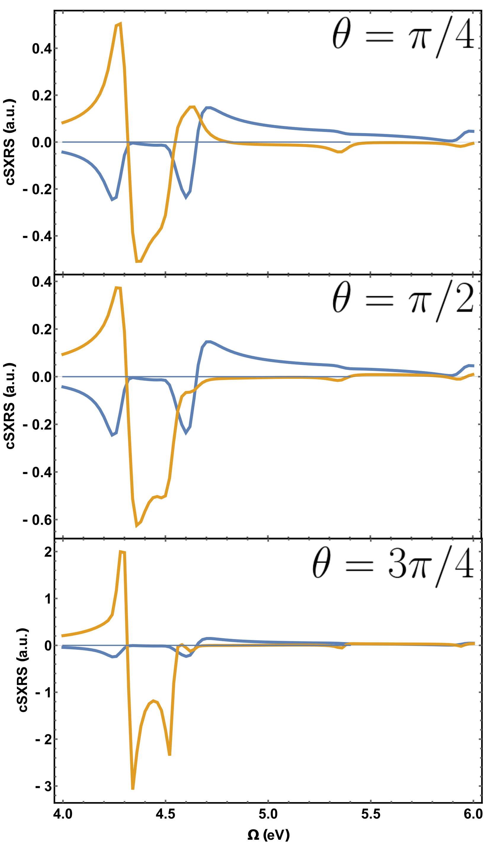
Figure 4: cSXRS($\Omega$,$\gamma$) for different crossing angles: $\pi/4$ (top), $\pi/2$ (middle) and $3\pi/4$ (bottom). Central frequencies are the same as in Fig. 3.

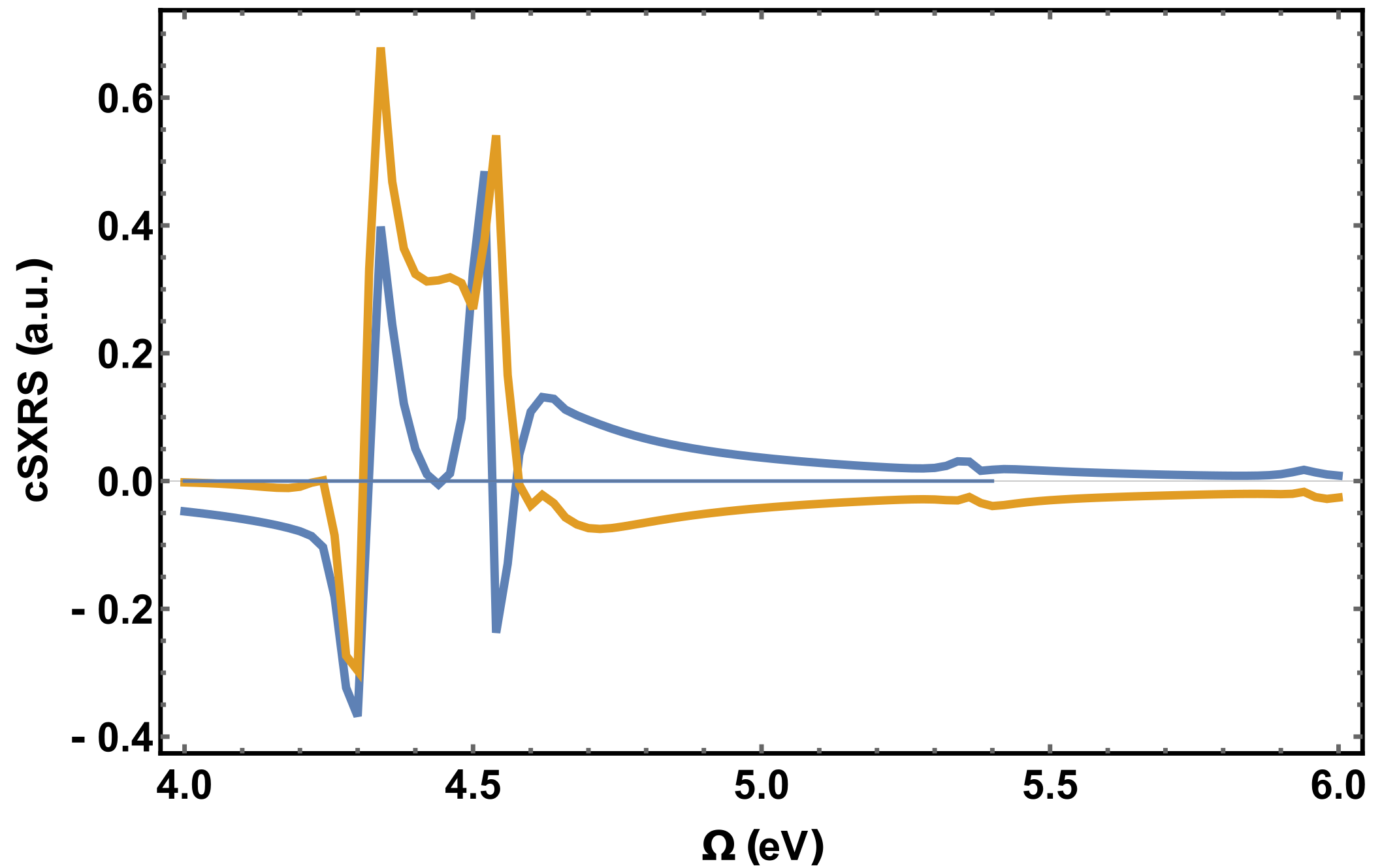
Figure 5: Sum of cSXRS signals with different crossing angles extracting pathways with a chiral interaction only during the first pulse (in blue, Eq. 25) or during the second pulse (in orange, Eq. 26).

Combining measurements with different crossing angles for the various chiral techniques ($\alpha$ or $\gamma$) allow to extract few selected contributions. For example, Fig. 5 shows SXRS signals in which the chiral interaction occurs only during the first pulse:

$$S_{\text{cSXRS}}(\Omega,\gamma,\frac{\pi}{4})-S_{\text{cSXRS}}(\Omega,\gamma,3\frac{\pi}{4})+S_{\text{cSXRS}}(\Omega,\alpha,\frac{\pi}{4})-S_{\text{cSXRS}}(\Omega,\alpha,3\frac{\pi}{4})=\\ -\Im\frac{2i}{15}\big{(}5\sqrt{6}\ _{1}R_{\mu\mu\mu m}-3\sqrt{5}_{1}R_{\mu\mu\mu q}+5\sqrt{6}_{1}R_{\mu\mu m\mu}\big{)}$$ (25)

or during the second pulse:

$$S_{\text{cSXRS}}(\Omega,\gamma,\frac{\pi}{4})-S_{\text{cSXRS}}(\Omega,\gamma,3\frac{\pi}{4})-(S_{\text{cSXRS}}(\Omega,\alpha,\frac{\pi}{4})-S_{\text{cSXRS}}(\Omega,\alpha,3\frac{\pi}{4}))=\\ -\Im\frac{2i}{15}\big{(}5\sqrt{6}\ _{1}R_{m\mu\mu\mu}+3\sqrt{5}_{1}R_{q\mu\mu\mu}+5\sqrt{6}_{1}R_{\mu m\mu\mu}\big{)}$$ (26)

3.3 Chiral 2D Electronic Spectroscopy

We next apply the 4WM polarization schemes to 2DES of S-ibuprofen. 2DES has been used to resolve excitonic couplings and energy transfer in molecular aggregates. It can further separate homogeneous and inhomogeneous contributions to absorption lineshapes. Here, we apply it to S-ibuprofen using phenomenological relaxation and compare with the SXRS signals that also probe the valence excited manifold. 2DES lacks the element-sensitivity of the X-rays but offers additional polarization and crossing angle controls because each interaction corresponds to a different pulse.

Figure 6: Ladder diagrams for 2DES.

We focus on 2DES non-rephasing ($\mathbb{k}_{II}$ technique) signals whose diagrams are given in Fig. 6. The correlation functions and SOS expressions of the 2DES signals are given in supplementary materials.

The freedom to independently select the polarization scheme and crossing angle for each of the four interactions results in a huge number of possible techniques. Here, we focus on a single case and other combinations can be computed using the supplementary materials. The chiral 2DES signal can be made to be sensitive to the electric quadrupole interaction only.

$$S_{\text{c2DES}}(\Omega_{1},T_{2},\Omega_{3},\alpha)=S_{\text{2DES}}(\Omega_{1},T_{2},\Omega_{3},LLLL)-S_{\text{2DES}}(\Omega_{1},T_{2},\Omega_{3},RRRR)$$ (27)

Using $,\theta_{1}=\pi/2,\theta_{2}=-\pi/2$ and $\theta_{3}=\pi/2$ as crossing angles, the pathways that contributes to the final signal are:

$$S_{\text{c2DES}}(\Omega_{1},T_{2},\Omega_{3},\alpha)=\frac{3\ _{1}R_{\mu q\mu\mu}-\sqrt{3}\ _{2}R_{\mu q\mu\mu}}{12\sqrt{10}}$$ (28)

Fig.7 compares the electric dipole contribution (panels a and b) with the quadrupole-sensitive c2DES signal. The dominant states in the achiral contribution (at 4.5 eV) are differnt from the ones in the chiral electric quadrupole one (at 4.3 eV). In SXRS, the 4.3 and 4.53 eV transitions were giving the main contributions to the signals. On the other hand, in the chiral 2DES signal displayed in Fig. 7 which contains only quadrupolar interactions, the 4.53 eV is contributing weakly.

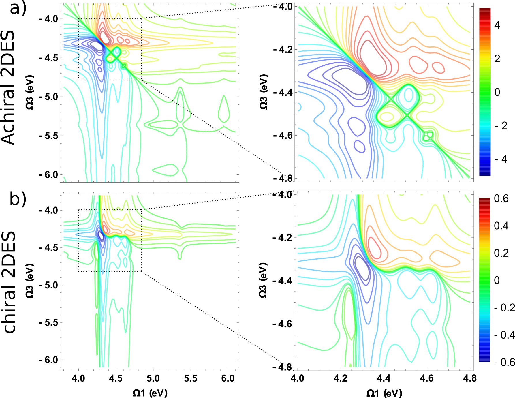
Figure 7: a) Achiral 2DES spectrum on an isotropic average (Eq. XX) of S-ibuprofen calculated in the dipolar approximation. b) Chiral 2DES defined in Eq. 27 with crossing angles $\theta_{1}=\pi/2,\theta_{2}=-\pi/2$ and $\theta_{3}=\pi/2$. This choice of polarization and crossing angles singles out only electric quadrupole interaction in the chiral interactions. The right panels show the main features on an expanded scale.

4 Conclusions

Chiral 4WM signals can combine the detailed information of 4WM techniques on molecular dynamics and relaxation with the inherent structural aspects of chirality. Their interpretation based on the multipolar expansion truncated at the magnetic dipole and electric quadrupole order is complicated by the many possible interaction pathways. We have used the irreducible tensor formalism to calculate each contribution to the signals for various pulse configurations and circularly polarized light.

Applications are made to two chiral-sensitive 4WM techniques, SXRS and 2DES. While the former is more restricted since multiple interactions occur with the same pulse, it allows to add the extra element-sensitivity of the X-rays. 2DES on the other hand uses optical or UV pulses but is a well-established tabletop technique that has better control of the crossing angles and pulses polarizations.

Some polarization configurations are identified which permit to isolate specific contributions in which the chiral interaction (with the magnetic dipole or with the electric quadrupole) occurs at a chosen step within the interaction pathways. We further have shown how to extract chiral contributions involving only the magnetic dipole or the electric quadrupole.

Appendix A Chiral-sensitive 4WM signals

${}_{\tau}\bm{R}_{\text{dip-E}}^{J=0}$ and ${}_{\tau}\bm{R}_{\text{dip-M}}^{J=0}$ are rank 4 tensors that have the following rotational invariants:

$${}_{0}R^{J=0} = \{\{\bm{A}\otimes\bm{B}\}_{0}\otimes\{\bm{C}\otimes\bm{D}\}_{0}\}_{0}=\frac{1}{3}(\bm{A}\cdot\bm{B})(\bm{C}\cdot\bm{D})$$ (29)

$${}_{1}R^{J=0} = \{\{\bm{A}\otimes\bm{B}\}_{1}\otimes\{\bm{C}\otimes\bm{D}\}_{1}\}_{0}=\frac{1}{\sqrt{3}}(\bm{A}\wedge\bm{B})\cdot(\bm{C}\wedge\bm{D})$$ (30)

$${}_{2}R^{J=0} = \{\{\bm{A}\otimes\bm{B}\}_{2}\otimes\{\bm{C}\otimes\bm{D}\}_{2}\}_{0}$$ (31)

$$= \frac{1}{\sqrt{5}}(\frac{1}{2}(\bm{A}\cdot\bm{C})(\bm{B}\cdot\bm{D})-\frac{1}{3}(\bm{A}\cdot\bm{B})(\bm{C}\cdot\bm{D})+\frac{1}{2}(\bm{A}\cdot\bm{D})(\bm{B}\cdot\bm{C}))$$ (32)

where $A,B,C$ and $D$ can be either an electric dipole $\bm{\mu}$ or a magnetic dipole $\bm{m}$ interaction. Each of these invariants gets contracted with the corresponding field invariants ${}_{\tau}F^{J=0}$:

$${}_{0}F(\bm{p}_{s},\bm{p}_{3},\bm{p}_{2},\bm{p}_{1})^{J=0} = \{\{\bm{p}_{s}\otimes\bm{p}_{3}\}_{0}\otimes\{\bm{p}_{2}\otimes\bm{p}_{1}\}_{0}\}_{0}$$ (33)

$${}_{1}F(\bm{p}_{s},\bm{p}_{3},\bm{p}_{2},\bm{p}_{1})^{J=0} = \{\{\bm{p}_{s}\otimes\bm{p}_{3}\}_{1}\otimes\{\bm{p}_{2}\otimes\bm{p}_{1}\}_{1}\}_{0})$$ (34)

$${}_{2}F(\bm{p}_{s},\bm{p}_{3},\bm{p}_{2},\bm{p}_{1})^{J=0} = \{\{\bm{p}_{s}\otimes\bm{p}_{3}\}_{2}\otimes\{\bm{p}_{2}\otimes\bm{p}_{1}\}_{2}\}_{0}$$ (35)

where $\bm{p}_{i}=\bm{\epsilon}_{i}$ or $\frac{i}{c}\bm{\hat{k}}_{i}\wedge\bm{\epsilon}_{i}$. ${}_{\tau}R_{\text{quad-E}}^{J=0}$ is a rank 5 tensor that has two rotational invariants:

$${}_{0}R_{\text{quad-E}}^{J=0} = \{\{\bm{\mu}\otimes\bm{\mu}\}_{1}\otimes\{\bm{\mu}\otimes\bm{q}\}_{1}\}_{0}$$ (36)

$${}_{1}R_{\text{quad-E}}^{J=0} = \{\{\bm{\mu}\otimes\bm{\mu}\}_{2}\otimes\{\bm{\mu}\otimes\bm{q}\}_{2}\}_{0}$$ (37)

The relevant field tensors are:

$${}_{0}G(\bm{a},\bm{b},\bm{c},i\bm{k}\otimes d)^{J=0} = \{\{\bm{a}\otimes\bm{b}\}_{1}\otimes\{\bm{c}\otimes\{i\bm{k}\otimes\bm{d}\}_{2}\}_{1}\}_{0}$$ (38)

$${}_{1}G(\bm{a},\bm{b},\bm{c},i\bm{k}\otimes d)^{J=0} = \{\{\bm{a}\otimes\bm{b}\}_{2}\otimes\{\bm{c}\otimes\{i\bm{k}\otimes\bm{d}\}_{2}\}_{2}\}_{0}$$ (39)

where $\bm{a},\bm{b},\bm{c},\bm{d}=\bm{\epsilon}_{i}$. We assume that the heterodyning pulse propagates along $z$ (hence $\bm{\hat{k}}_{s}=\bm{e}_{0}$). The three exciting pulses are non-collinear, forming an angle $\theta_{i}$ with the $y$ axis. This corresponds to the most common experimental situation where multiple pulses parallel to the optical table are incident on the sample with a small angle between them. We further assume that the electric field polarization $\bm{\epsilon}_{1},\bm{\epsilon}_{2},\bm{\epsilon}_{3}$ are left or right polarized in the laboratory frame. In the irreducible basis $\{\bm{e}_{1},\bm{e}_{0},\bm{e}_{-1}\}$, the polarization vectors are given by

$$\bm{e}_{L}=\begin{pmatrix}1\\ 0\\ 0\end{pmatrix}\ \ \ \ \ \ \ \bm{e}_{R}=\begin{pmatrix}0\\ 0\\ 1\end{pmatrix}$$ (40)

where $\bm{e}_{L}$ and $\bm{e}_{R}$ are the left and right-handed polarization vectors for a plane wave propagating along $z$. For non-collinear pulses, the Wigner $\mathcal{D}^{J=1}$ matrix can be used to obtain the corresponding left and right polarizations. The vectors $(\bm{e}_{L},\bm{e}_{R},\bm{e}_{z})$ form an orthonormal basis with the following properties:

$$\bm{e}_{L}^{*}=-\bm{e}_{R}\hskip 68.28644pt\bm{e}_{R}^{*}=-\bm{e}_{L}$$

$$\bm{e}_{L}\cdot\bm{e}_{L}=\bm{e}_{R}\cdot\bm{e}_{R}=0\hskip 14.22636pt\bm{e}_{L}\cdot\bm{e}_{R}=-1$$

$$\bm{e}_{z}\times\bm{e}_{L}=-i\bm{e}_{L}\hskip 39.83368pt\bm{e}_{z}\times\bm{e}_{R}=i\bm{e}_{R}$$ (41)

Eq. 41 allows to get the polarization vectors $\bm{b}$ of the magnetic field

$$\bm{b}_{L/R}=\frac{1}{c}\bm{e}_{z}\times\bm{e}_{L/R}$$ (42)

In supplementary materials, we give the non-vanishing tensor components corresponding to different polarization schemes and the general tensor expressions for arbitrary polarization vectors in term of Clebsch-Gordan sums.

2 Supporting Information

Details on the quantum chemistry of S-ibuprofen and on the 2DES and SXRS signal derivations are given in supplementary materials. The program allowing to extract the response tensor irreducible components contributing to a given configuration is also available.

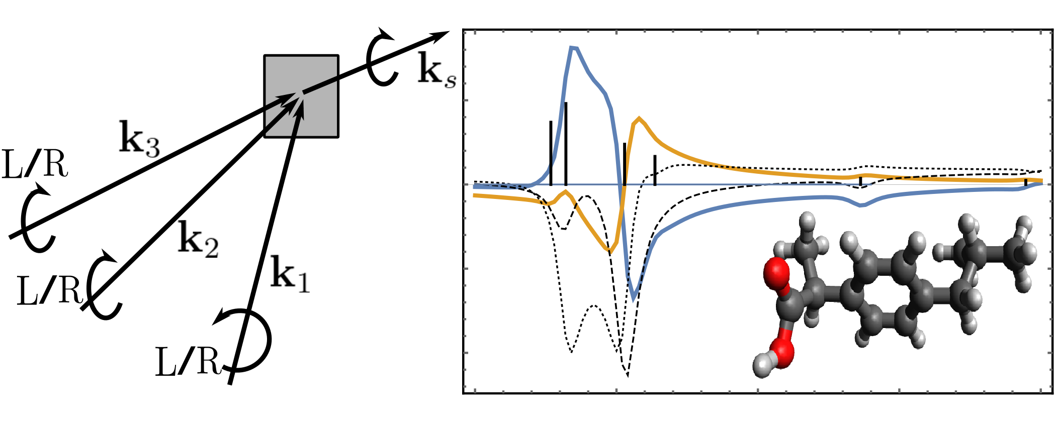
Figure 8: TOC graphics

References

- Quack 2002 Quack, M. How important is parity violation for molecular and biomolecular chirality? Angewandte Chemie International Edition 2002, 41, 4618–4630
- Flügel 2011 Flügel, R. M. Chirality and Life: A Short Introduction to the Early Phases of Chemical Evolution; Springer Science & Business Media, 2011
- Francotte and Lindner 2006 Francotte, E.; Lindner, W. Chirality in drug research; Wiley-VCH Weinheim, 2006; Vol. 33
- Berova et al. 2000 Berova, N.; Nakanishi, K.; Woody, R. W. Circular dichroism: principles and applications; John Wiley & Sons, 2000
- He et al. 2011 He, Y.; Bo, W.; Dukor, R. K.; Nafie, L. A. Determination of absolute configuration of chiral molecules using vibrational optical activity: a review. Applied Spectroscopy 2011, 65, 699–723
- Barron 2009 Barron, L. D. Molecular light scattering and optical activity; Cambridge University Press, 2009
- Powis 2008 Powis, I. Photoelectron circular dichroism in chiral molecules. Advances in Chemical Physics 2008, 138, 267–330
- Hache et al. 1999 Hache, F.; Mesnil, H.; Schanne-Klein, M. Nonlinear circular dichroism in a liquid of chiral molecules: A theoretical investigation. Physical Review B 1999, 60, 6405
- Abramavicius et al. 2009 Abramavicius, D.; Palmieri, B.; Voronine, D. V.; Sanda, F.; Mukamel, S. Coherent multidimensional optical spectroscopy of excitons in molecular aggregates; quasiparticle versus supermolecule perspectives. Chemical reviews 2009, 109, 2350–2408
- Fischer and Hache 2005 Fischer, P.; Hache, F. Nonlinear optical spectroscopy of chiral molecules. Chirality: the pharmacological, biological, and chemical consequences of molecular asymmetry 2005, 17, 421–437
- Mesnil and Hache 2000 Mesnil, H.; Hache, F. Experimental evidence of third-order nonlinear dichroism in a liquid of chiral molecules. Physical review letters 2000, 85, 4257
- Belkin and Shen 2005 Belkin, M.; Shen, Y. Non-linear optical spectroscopy as a novel probe for molecular chirality. International Reviews in Physical Chemistry 2005, 24, 257–299
- Castiglioni et al. 2009 Castiglioni, E.; Biscarini, P.; Abbate, S. Experimental aspects of solid state circular dichroism. Chirality: The Pharmacological, Biological, and Chemical Consequences of Molecular Asymmetry 2009, 21, E28–E36
- Craig and Thirunamachandran 1998 Craig, D. P.; Thirunamachandran, T. Molecular quantum electrodynamics: an introduction to radiation-molecule interactions; Courier Corporation, 1998
- Andrews and Ghoul 1982 Andrews, D.; Ghoul, W. Irreducible fourth-rank Cartesian tensors. Physical Review A 1982, 25, 2647
- Jerphagnon et al. 1978 Jerphagnon, J.; Chemla, D.; Bonneville, R. The description of the physical properties of condensed matter using irreducible tensors. Advances in Physics 1978, 27, 609–650
- Mun and Rho 2019 Mun, J.; Rho, J. Importance of higher-order multipole transitions on chiral nearfield interactions. Nanophotonics 2019, 8, 941–948
- Rusak et al. 2019 Rusak, E.; Straubel, J.; Gładysz, P.; Göddel, M.; Kȩdziorski, A.; Kühn, M.; Weigend, F.; Rockstuhl, C.; Słowik, K. Enhancement of and interference among higher order multipole transitions in molecules near a plasmonic nanoantenna. Nature communications 2019, 10, 1–8
- Yamamoto 2008 Yamamoto, T. Assignment of pre-edge peaks in K-edge x-ray absorption spectra of 3d transition metal compounds: electric dipole or quadrupole? X-Ray Spectrometry: An International Journal 2008, 37, 572–584
- Berera et al. 2009 Berera, R.; van Grondelle, R.; Kennis, J. T. Ultrafast transient absorption spectroscopy: principles and application to photosynthetic systems. Photosynthesis research 2009, 101, 105–118
- Harbola and Mukamel 2008 Harbola, U.; Mukamel, S. Superoperator nonequilibrium Green’s function theory of many-body systems; applications to charge transfer and transport in open junctions. Physics Reports 2008, 465, 191–222
- Varshalovich et al. 1988 Varshalovich, D. A.; Moskalev, A. N.; Khersonskii, V. K. Quantum theory of angular momentum; World Scientific, 1988
- Werner et al. 2012 Werner, H.-J.; Knowles, P. J.; Knizia, G.; Manby, F. R.; Schütz, M. Molpro: a general-purpose quantum chemistry program package. Wiley Interdisciplinary Reviews: Computational Molecular Science 2012, 2, 242–253
- Reiher 2006 Reiher, M. Douglas–Kroll–Hess Theory: a relativistic electrons-only theory for chemistry. Theoretical Chemistry Accounts 2006, 116, 241–252
- Moore 2002 Moore, D. E. Photophysical photochemical and aspects of drug stability. 2002, 19–48
- Mincigrucci et al. 2020 Mincigrucci, R.; Rouxel, J. R.; Rossi, B.; Principi, E.; Bottari, C.; Catalini, S.; Fainozzi, D.; Foglia, L.; Simoncig, A.; Matruglio, A.; Kurdi, G.; Capotondi, F.; Pedersoli, E.; Perucchi, A.; Piccirilli, F.; Gessini, A.; Giarola, M.; Mariotto, G.; Mukamel, S.; Bencivenga, F.; Chergui, M.; Masciovecchio, C. Element and enantiomeric selective visualization of ibuprofen dimer vibrations; submitted for publication, 2020