Improving Recurrent Neural Network Responsiveness to Acute Clinical Events

Abstract

Predictive models in acute care settings must be able to immediately recognize precipitous changes in a patient’s status when presented with data reflecting such changes. Recurrent neural networks (RNN) have become common for training and deploying clinical decision support models. They frequently exhibit a delayed response to acute events. New information must propagate through the RNN’s cell state memory before the total impact is reflected in the model’s predictions. This work presents input data perseveration as a method of training and deploying an RNN model to make its predictions more responsive to newly acquired information: input data is replicated during training and deployment. Each replication of the data input impacts the cell state and output of the RNN, but only the output at the final replication is maintained and broadcast as the prediction for evaluation and deployment purposes. When presented with data reflecting acute events, a model trained and deployed with input perseveration responds with more pronounced immediate changes in predictions and maintains globally robust performance. Such a characteristic is crucial in predictive models for an intensive care unit.

1 Introduction

1.1 The Problem

Critical care environments require rapid decision making. To be meaningful, predictive models in these settings must immediately recognize precipitous changes in a patient’s state when presented with data reflecting such changes [1, 2]. Newly acquired information must be integrated quickly with the existing understanding of the patient’s state to inform clinical decisions.

Long Short-Term Memory (LSTM) models [3] are a type of Recurrent Neural Network (RNN) architecture and have become increasingly popular for modeling tasks in clinical settings, including Intensive Care Units (ICUs) [4, 5, 6, 7, 8, 9, 10, 11]. It is occasionally noted that RNNs, including LSTM models, exhibit some lag after acquiring new information [12]. This characteristic is frequently observed in stock prediction tasks where the apparent predictive capability of a model is comparable to a model that predicts the last observed stock price [13, 14]. However, the intersection of deep learning and healthcare, though ever widening, has a paucity of literature on this phenomenon. Commonly reported metrics such as Area Under the Receiver Operating Characteristic Curve, sensitivity, specificity, and mean absolute errors mask certain behaviors of RNN based models.

RNN models require computational cycles to incorporate new data into their memory cell [15]. There are two primary observable effects of this, summarized briefly here. First, what we refer to as a pipe-up period, requires the initial input to propagate through the memory cell to overcome the initialized cell state before that input significantly influences the predictions. Second, during all subsequent times, new information only slightly changes the overall prediction of a model at the time of input and requires propagation through the memory cell before fully augmenting the model’s prediction. The first phenomenon is a special case of the second. These two effects are further illustrated in Sections 5 and 6.

1.2 Proposed Solution

This work aims to enable more pronounced changes in RNN predictions when the model is presented with data indicating acute clinical events by perseverating the input. Instead of giving newly available input data to an RNN model only once, the input is replicated and given to the model multiple times, during both training and deployment, with only the prediction of the final perseveration maintained and made visible to the end-user. This approach provides additional computational cycles for new data to be incorporated into the model’s internal states before a prediction is broadcast. We hypothesized that the resultant model would be able to react to acute events more quickly than traditionally trained LSTMs and still maintain overall model performance.

2 Related Works

Since the seminal paper by R.E. Kalman in 1960 describing what is now called the Kalman Filter [16], engineers have been aware of the trade off between integrating historical data and responding to new data. Most training techniques used in modern deep learning affect the balance between relying on historical trends and responding to new information; such techniques include dropout, optimizers, and activation functions [17, 18, 19, 20]. Generating an appropriate target vector (e.g. using changes in values between consecutive time points instead of predicting raw values) is another training technique that can prevent generation of an auto-correlation model [12].

Attention mechanisms [21] are sometimes used to manage the balance between historical and new data by appending the entire input sequence to the final hidden layer of an RNN. Doing so affords the model another opportunity to learn weights which expose the moments in time series data most relevant to the predictions. Attention networks were originally developed for post-hoc sequence-to-sequence modeling tasks such as image captioning and neural machine translation which permit access to the entire input sequence when making predictions [22, 21]. An attention mechanism was applied by Zhang, et al. to predict risk of future hospitalization using medical records from a fixed observation window.[23].

3 Data

3.1 Clinical Data Sources

Data for this work were extracted from de-identified observational clinical data collected in Electronic Medical Records (EMR, Cerner) in the Pediatric Intensive Care Unit (PICU) of Children’s Hospital Los Angeles (CHLA) between January 2009 and February 2019. The CHLA Institutional Review Board (IRB) reviewed the study protocol and waived the need for IRB approval. A patient record included static information such as gender, race, and discharge disposition at the end of an ICU episode, defined as a contiguous admission in the PICU. A patient may have multiple episodes. The EMR for an episode also contained irregularly, sparsely and asynchronously charted measurements of physiologic observations (e.g. heart rate, blood pressure), laboratory results (e.g. creatinine, glucose level), drugs (e.g. epinephrine, furosemide) and interventions (e.g. intubation, oxygen level). Episodes without discharge disposition were excluded, leaving 12,826 episodes (9,250 patients) in the final dataset.

Prior to any of the computational experiments described here, the episodes were randomly partitioned into three sets: a training set for deriving model weights, a validation set for optimizing hyper-parameters, and a holdout test set for measuring performance. To minimize bias in the performance evaluation metrics, partitioning was done at the patient level, i.e. all episodes from a single patient belonged to only one of these sets: 60% in the training set, 20% in the validation set, and 20% in the test set. No other stratification was applied. Table I displays basic characteristics of the resulting data partitions.

Preprocessing steps described in previous work [24] converted each episode data to a matrix structure amenable to machine learning model development. A row of values in this matrix represented measurements (recorded or imputed) of different variables at one particular time, while a column contained values of a single variable at different times. A complete list of variables used as model inputs can be found in Appendix A. Note that diagnoses, while available in the EMR, were not used as input features.

TABLE I: Basic demographics of data used in this study for each data partition.

	training	validation	test	overall
Number of episodes	7663	2541	26221	12826
Number of patients	5551	1850	18501	9251
Mortality rate	0.035	0.037	0.043	0.037
Fraction male	0.56	0.55	0.58	0.56
Age mean (years)	7.99	8.23	8.09	8.06
std dev	6.45	6.51	6.35	6.44

3.2 Target Outcome

ICU mortality was chosen as the target outcome because it is a simple, unambiguous outcome. Importantly, risk of mortality is used commonly as a proxy for severity of illness in critical care [25, 26, 27, 28]. The overall mortality rate of the data was $3.7\%$ (Table I).

4 RNN Models

Many-to-many recurrent neural network models, consisting of stacked Long Short-Term Memory (LSTM) layers followed by a dense layer, were trained to predict ICU mortality of each patient episode. All the models output a probability of survival at each distinct time point where an observation or measurement of the patient was made, generating a trajectory of scores that reflect the changing status of a patient during their ICU episode.

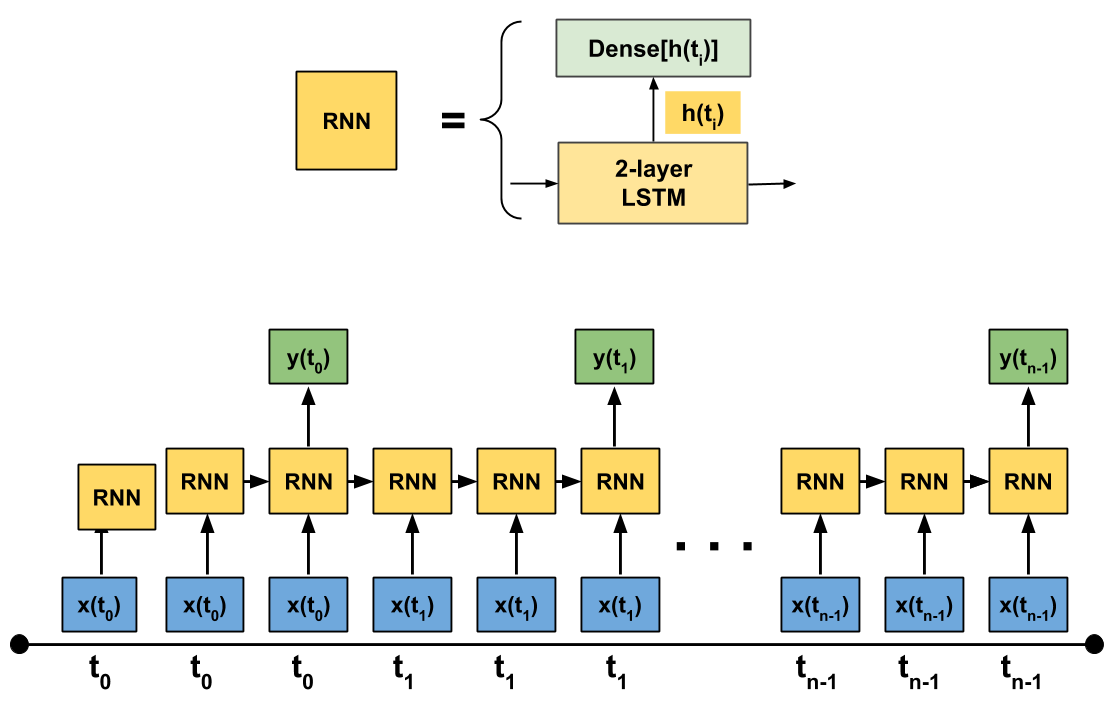
Figure 1: The perseverating recurrent neural network (PRNN) is an RNN with repeating inputs. Each input vector associated with a particular time is replicated $k$ times, and only the output from the last replication is considered as the prediction for that time. The diagram above illustrates the process for $k=3$.

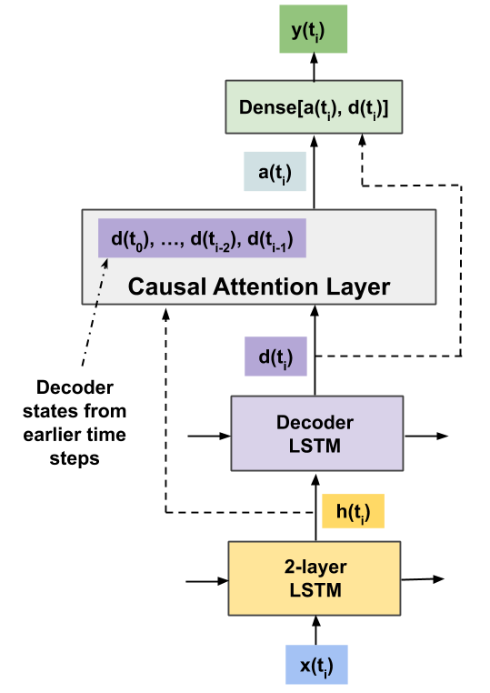
Figure 2: Overview of a standard RNN model with a causal attention layer.

The baseline RNN model was trained in the traditional manner: when the model acquires new data $x(t_{i})$, it generates and immediately broadcasts a prediction $y(t_{i})$. Other models which share the architecture of the baseline RNN model were trained using input perseveration: the same $x(t_{i})$ vector was repeatedly given as input to the RNN model $k$ times, where $k$ is a controllable parameter. While all $k$ outputs – corresponding to the $k$ times that $x(t_{i})$ was given to the model – are used for optimization during training, only the last one is maintained and broadcast as the prediction at time $t_{i}$ during performance assessment and deployment. We call these models perseverating recurrent neural networks (PRNN). Figure 1 illustrates a PRNN model with $k=3$. Note that the baseline RNN can be considered as a PRNN with $k=1$. Input perseveration provides the internal cell state memory of the RNN additional computational cycles to incorporate the current state of the patient into the final prediction.

An attention network using the same hyperparameters of the baseline RNN model was also implemented. Most attention networks have access to the entire sequence of inputs – both past and future relative to the current one – when making a prediction at any point in time. However, continuous monitoring of patient status precludes access to future information, available in a retrospective study but not in a real deployment scenario. Therefore, the attention layer between the last hidden layer and output layer used a causal mask that exposed only the inputs up to the time when a prediction is being made [29]. This ensured that the network did not use future information to make its predictions while affording it another opportunity to consider the totality of information up to the current time. See Figure 2 for a diagram of the model.

All six models – baseline RNN ($k=1$), PRNN for $k=2,3,4,5$, and attention RNN – were implemented and trained using Keras 2.0.7 with the Theano 1.0.2 backend [30, 31]. For each model, weights were optimized on the training and validation sets; performance was computed on the validation set after every epoch (i.e. a full cycle through the training set), and the best performing weights were saved as the final model. Table II displays the hyperparameters that were used for all six models. The final models were assessed for performance metrics on the test set.

TABLE II: Hyperparameters for all permutations of the PRNN.

Hyperparameter	Value
Number of LSTM Layers	3
Hidden Units in LSTM Layers	[128, 256, 128]
Batch Size	32
Initial Learning Rate	1e-5
Loss	binary cross-entropy
Optimizer	rmsprop
Dropout	0.2
Recurrent Dropout	0.2
Regularizer	0.0001
Output Activation	sigmoid

5 Model Assessments

Standard metrics such as the Area Under the Receiver Operating Characteristic Curve (AUROC), precision, and recall scores for a binary classification task can capture a model’s overall predictive performance. However, they can mask the lag phenomenon displayed by LSTMs that, although known, is rarely commented on in the literature. The trajectory of probability of survival predictions should reflect the evolving state of a patient which can have instantaneous changes. Metrics were designed to quantify a model’s pipe-up behavior and its ability to capture rapid changes resulting from clinically adverse events. AUROC was used to compare overall predictive performance for the main task – ICU mortality prediction.

5.1 Pipe-Up Behavior

A model’s prediction at the first time step is a function of its weights, initial state of its memory cells and the first input. Of these, only the first input varies across different patient episodes; therefore, the distribution of a model’s prediction at the first time point of all episodes indicates the model’s level of reliance on the first input data. We refer to this period as the pipe-up period.

The mean and standard deviation of the distribution of all $\hat{y}_{p}(t_{0})$ predictions, where $\hat{y}_{p}(t_{0})$ represents the first prediction for patient episode $p$, were computed for all survivors and non-survivors in the test set. These metrics were computed for all six RNN models described in the previous section and used to compare their responsiveness to the first available information about a patient episode.

5.2 Responsiveness to Acute Events

The models were also assessed for their instantaneous responses to clinically adverse events using an average variation metric computed from the predictions during such periods. In consultation with clinicians, the times when any of the following occurred were defined as acute time points or intervals:

1. substantial increases in creatinine levels or inotrope score between two consecutive recordings;

2. substantial decreases in heart rate, mean arterial pressure, Glasgow Coma Score, blood oxygen level (SpO2), arterial blood gas (ABG) pH, and venous blood gas (VBG) pH between two consecutive recordings;

3. a patient’s heart rate goes to 0.

We quantified substantial changes as those that were in the top or bottom $X$ percentile ($X\in\{5.0,1.0,0.5\}$) of inter-measurement changes. For example, a time point $t_{i}$ was considered acute in terms of creatinine when the increase in creatinine level from $t_{i-1}$ to $t_{i}$ was in the top $X$ percentile of all creatinine level percent changes between any two consecutive time points in the test dataset. Similarly, acute time points for heart rate were those times when the decrease in heart rate was in the bottom $X$% of all heart rate changes between any two consecutive time points of all test set episodes. Table III shows the specific percent change thresholds indicating acute changes in a patient. Thus, a 32% drop in heart rate between two consecutive measurements would be in the top 1 percentile, while a 70% increase in inotrope score would be in the top 5 percentile.

Applying three percentile-based thresholds to define acute patient state changes meant a total of 25 acuity definitions (2 * 3 increases in measured variables, 6 * 3 decreases in measured variables, and zero heart rate) used to assess models’ responses when such events occur. It is important to note that we are not proposing these as general definitions of clinical acuity. They were designed to capture events that indicate precipitous changes in a patient’s state with high specificity to assess the magnitude of the instantaneous change in predicted probability of survival.

Each previously defined acute event, denoted by $E$, identified a set of acute time points, denoted by $S_{E}(p)$, for each patient episode $p$. Changes in a model’s prediction at these time points were evaluated through an average temporal variation metric given by:

$$V_{E}(p) = \frac{100}{|S_{E}(p)|}\sum_{t_{i}\in S_{E}(p)}|\hat{y}_{p}(t_{i})-\hat{y}_{p}(t_{i-1})|,$$ (1)

where $\hat{y}_{p}(t_{i})$ is the prediction for patient episode $p$ at time point $t_{i}$, and $|S_{E}(p)|$ is the number of time points in $S_{E}(p)$. This metric measures how much the predicted probability of survival (scaled to $[0,100]$) changed, on average, at the defined acute time points of an episode. Model $A$ having a higher $AV(p)$ than model $B$ means that when both models were presented with data reflecting a precipitous change in a patient’s state, model $A$’s prediction underwent a greater change than model $B$’s prediction, indicating that model $A$ had a more pronounced response to the acute event. The average of this metric across $N_{p}$ episodes gives a measure of the model’s overall responsiveness to acute event $E$ of those episodes:

$$\bar{V}_{E}=\frac{1}{N_{p}}\sum_{p}V_{E}(p).$$ (2)

TABLE III: Thresholds of percent change used to define acute changes in patient state. Negative thresholds correspond to the bottom $p\%$ of changes and positive thresholds correspond to the top $p\%$ of changes, for $p\in[5,1,0.5]$.

	5%	1%	0.5%
Heart Rate	-18.8	-31.6	-37.1
Mean Arterial Pressure	-23.5	-38.1	-44.2
Glascow Coma Score	-50.0	-72.7	-72.7
Pulse Oximetry	-5.6	-20.2	-35.1
ABG pH	-1.5	-2.9	-3.5
VBG pH	-1.4	-2.6	-3.1
Inotrope Score	66.7	150.0	250.0
Creatinine	33.3	60.5	81.8

5.3 Overall Predictive Performance

Model predictions at ICU admission and at 1, 3, 6, 12, and 24 hours after ICU admission were evaluated for predictive performance via the AUROC. Performance was only measured for episodes lasting at least $24$ hours to maintain a consistent cohort across time slices ($n=2130$, mortality rate = 0.046).

6 Results

Figure 3 illustrates trajectories of probability of survival predictions from two models, the baseline RNN ($k=1$) and a PRNN with $k=5$, for two non-surviving episodes. In the first episode (top), the patient had a rapid increase of creatinine level, which indicates kidney dysfunction, about 500 hours after ICU admission. When presented with this defined acute event, the baseline model’s prediction dropped from 0.89 to 0.88, while the PRNN model dropped from 0.75 to 0.71. In the second episode (bottom), the patient’s Glasgow Coma Score decreased from 7 to 4. When presented with this defined acute event, the baseline model’s probability of survival prediction dropped from 0.76 to 0.70, while the PRNN model dropped from 0.69 to 0.50. In either case, the PRNN model’s immediate response to an acute event was more pronounced than that of the baseline RNN model. Further, the trajectory of the baseline RNN’s predictions after either acute event appears to lag behind that of the PRNN by about 1-2 hours.

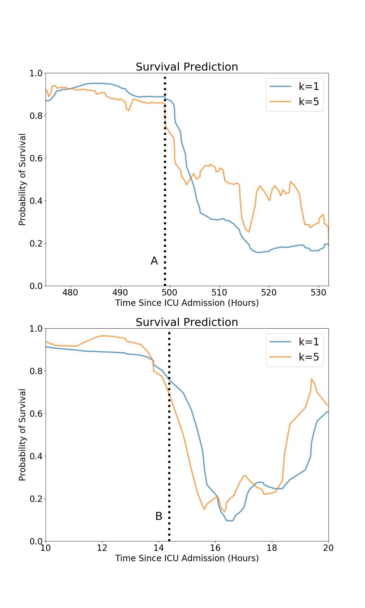
Figure 3: Two examples of predictions following acute events in two individual patient episodes. The blue curves correspond to the baseline ($k=1$) model, while the orange curves correspond to the PRNN model with $k=5$. The dotted vertical lines denote onset of an acute event for each patient: (A) a patient experiencing kidney failure and the moment of increased creatinine and blood urea nitrogen (BUN); (B) a patient’s Glasgow Coma Score decreasing from 7 to 4, indicating significantly reduced levels of consciousness.

The remainder of this section describes the results from aggregating the assessment metrics described in Section 5 across episodes in the test dataset.

Figure 4: Distribution of model predictions at the first available observation for survivors and non-survivors

6.1 Pipe-Up Behavior

Figure 4 shows the distribution of predictions at the first observation. The mean prediction for survivors increased with the perseveration parameter $k$: from $0.70$ ($k=1$) to $0.90$ ($k=5$). For both survivors and non-survivors, the standard deviation increased with $k$. The increase of standard deviation was more pronounced in the non-survivors, going from from $0.04$ at $k=1$ to $0.13$ at $k=5$.

6.2 Responsiveness to Acute Events

Figure 5 displays the average variation as a function of $k$ and acuity definitions. Two trends are apparent. First is the behavior of average variation as a function of percentile change in a given physiologic observation or intervention. For each model, the resulting average variation increased as the change in a physiologic or intervention variable became more severe (ie. from 95.0 to 99.5 percentile). Second, a clear positive correlation between $k$ and average variation is evident across all definitions of acuity. The attention layer generally demonstrated lower average variation than the $k=1$ model.

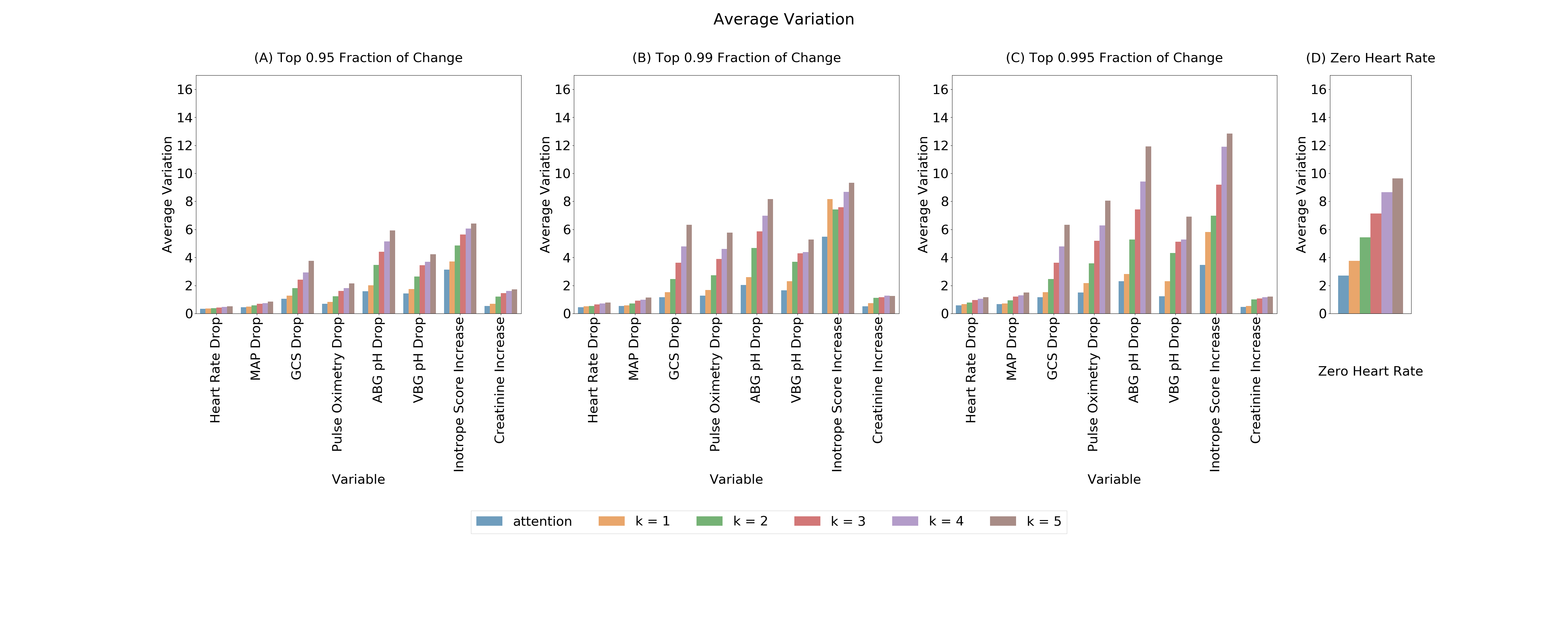
Figure 5: Comparison of the average variation metric $\bar{V}_{E}$ of different models as defined by Equation 2 across all test set episodes, where the events are defined by: A) a 95th percentile change; B) a 99th percentile change; C) a 99.5th percentile change; D) a cardiac arrest.

6.3 Overall Predictive Performance

Table IV summarizes the AUROC of model predictions at different times after ICU admission of all episodes in the test set that lasted at least 24 hours. The AUROC gains due to input perseveration were larger at the earlier times of prediction ($t\leq 6$ hours), increasing at the first hour from $0.77$ when $k=1$ to $0.83$ when $k=5$. By the 12th hour, the AUROC did not significantly change with the perseveration parameter $k$. Performance increases for all models as additional hours of observation are available. Adding an attention layer displayed similar performance as the baseline model ($k=1$) at all evaluation times.

TABLE IV: Test set AUROCs for the mortality prediction at admission and after $1$, $3$, $6$, $12$, and $24$ hours of observation. Only the patient episodes lasting at least $24$ hours of ICU time were evaluated.

k	0hr	1hr	3hr	6hr	12hr	24hr
1	0.716	0.766	0.859	0.895	0.914	0.952
2	0.729	0.804	0.871	0.902	0.916	0.956
3	0.731	0.819	0.875	0.902	0.916	0.955
4	0.735	0.821	0.876	0.900	0.915	0.954
5	0.736	0.832	0.883	0.905	0.919	0.955
attention	0.723	0.734	0.853	0.892	0.910	0.949

7 Discussion

Real time predictions for ICU mortality are proxies for severity of illness [28, 32, 33] and should reflect acute changes in a patient. The examples in Figure 3 show that the mortality model trained with input perseveration (PRNN with $k=5$) responded more pronouncedly and immediately than the traditionally trained model ($k=1$) when both were presented with data reflecting acute changes. Subsequent to the acute changes, the responses of the traditional RNN appeared to lag behind the PRNN’s. Standard metrics such as AUROCs for classification or mean absolute errors for continuous regression often mask this predictive lag and other deleterious behaviors that can be detrimental in critical or intensive care settings where rapid recognition and response are crucial.

Input perseveration provides the RNN’s internal cells additional computational cycles to incorporate the current state of the patient into the final prediction. The effect of this method was measured by metrics designed to capture a model’s immediate responses to newly acquired data.

The variation metric described in Section 5.2 compares the models’ immediate responses to data indicating precipitous changes in a patient’s status. These changes require quick reaction time from the care team, therefore capturing them in the predictions is important. The comparison of variation metrics from the different models (Figure 5) shows that the LSTM became more responsive to acute clinical events as the level of perseveration, $k$, increased. When $k$ increased from 1 to 5, the variation metric corresponding to the defined precipitous events increased by a factor of 2-3 times. They also show that a given model’s responsiveness increased with more acute events (i.e. those belonging to higher percentile changes for a given physiologic or intervention variable). This result is consistent with expectations about the variation metric. For example, one would expect the change in predictions of those with larger drops in blood gas level to be greater than those of less severe drops.

Figure 4 compares the distributions of initial predictions generated by the different models. Since the first prediction is a function of both the initial input (which varies across episodes) and the initial cell state memory (which is fixed), a wider distribution of these predictions across episodes indicates a higher reliance on the initial input. This is important because children admitted to the PICU have different severities of illness [25, 27]. Increasing $k$ resulted in a wider distribution as measured by the standard deviation. The increase was greater for the non-surviving population ($\sigma=0.04$ when $k=1$ to $\sigma=0.13$ when $k=5$) relative to the surviving population. This is again consistent with clinical expectations.

Increasing the first prediction’s reliance on the initial measurement – as achieved by the PRNN models with higher $k$ – also resulted in higher AUROC at ICU admission (Table IV). As the models observed the patient longer, their AUROCs increased as expected. Importantly, the increase of AUROC due to perseveration was greater at the early hours ($t\leq 3$) when information is most scarce, with the 1-hour AUROC increasing from 0.77 when $k=1$ to 0.83 when $k=5$. This means that predictive clinical models relying on scarce data for early detection could benefit from the perseveration approach.

Adding a causal attention layer to the baseline ($k=1$) model had no apparent performance improvement in any of the metrics. The attention network theoretically can put more weight to the most recent state than to the previous ones. The results indicate that this mechanism did not improve on what the baseline LSTM’s gates were already doing, but persistently giving the same input to the model – i.e. perseverating the input – did.

There are limitations to the perseverated input approach. Although LSTMs are theoretically good at understanding temporal trends through their memory cells, there remain practical limitations to how long prior information can be maintained to inform future predictions [34, 35]. The PRNN has the potential to exacerbate these algorithmic deficiencies because of the memory cell’s prolonged exposure to the same data. A comprehensive assessment of the impact of a potential reduction in temporal memory was not performed. However, the basic data perseveration technique can easily be generalized to any sequential data.

Additionally, perseveration increases the number of sequences requiring computation. Perseveration is used during both training and inference, and the compute time scales linearly for both, commensurate with the level of perseveration. However, the time required for inference is on the order of $30ms$ for $k=1$ (baseline) and $150ms$ for $k=5$ on an NVIDIA Titan RTX. Since the recording frequency is approximately every 15 minutes, these computational burdens do not hinder deployment.

Finally, this proof-of-concept study used only a single clinical outcome (ICU mortality) and data from a single center. Future work will examine the effect of perseverating the data input on other important clinical tasks such as risk of desaturation, sepsis, and renal failure.

8 Conclusion

This work demonstrates that perseverated data input increases the responsiveness of LSTM models to a variety of acute changes to patient state and also significantly increases predictive performance in the early hours following admission. The PRNN is a simple solution to the predictive lag exhibited by standard LSTMs when encountering an acute event and may enable more rapid responses to critical conditions.

Appendix A EMR Variables

TABLE V: EMR variables (demographics, vitals and labs) in patient episode matrix. Demographics such as gender and race/ethnicity were encoded as binary variables.

Demographics and Vitals
Age	Sex_F	Sex_M	race_African American
race_Asian/Indian/Pacific Islander	race_Caucasian/European Non-Hispanic	race_Hispanic	race_unknown
Abdominal Girth	FLACC Pain Face	Left Pupillary Response Level	Respiratory Effort Level
Activity Level	FLACC Pain Intensity	Level of Consciousness	Respiratory Rate
Bladder pressure	FLACC Pain Legs	Lip Moisture Level	Right Pupil Size After Light
Capillary Refill Rate	Foley Catheter Volume	Mean Arterial Pressure	Right Pupil Size Before Light
Central Venous Pressure	Gastrostomy Tube Volume	Motor Response Level	Right Pupillary Response Level
Cerebral Perfusion Pressure	Glascow Coma Score	Nasal Flaring Level	Sedation Scale Level
Diastolic Blood Pressure	Head Circumference	Near-Infrared Spectroscopy SO2	Skin Turgor_edema
EtCO2	Heart Rate	Nutrition Level	Skin Turgor_turgor
Extremity Temperature Level	Height	Oxygenation Index	Systolic Blood Pressure
Eye Response Level	Hemofiltration Fluid Output	PaO2 to FiO2	Temperature
FLACC Pain Activity	Intracranial Pressure	Patient Mood Level	Verbal Response Level
FLACC Pain Consolability	Left Pupil Size After Light	Pulse Oximetry	WAT1 Total
FLACC Pain Cry	Left Pupil Size Before Light	Quality of Pain Level	Weight
Labs
ABG Base excess	CBG PCO2	GGT	Neutrophils %
ABG FiO2	CBG PO2	Glucose	PT
ABG HCO3	CBG TCO2	Haptoglobin	PTT
ABG O2 sat	CBG pH	Hematocrit	Phosphorus level
ABG PCO2	CSF Bands%	Hemoglobin	Platelet Count
ABG PO2	CSF Glucose	INR	Potassium
ABG TCO2	CSF Lymphs %	Influenza Lab	Protein Total
ABG pH	CSF Protein	Lactate	RBC Blood
ALT	CSF RBC	Lactate Dehydrogenase Blood	RDW
AST	CSF Segs %	Lactic Acid Blood	Reticulocyte Count
Albumin Level	CSF WBC	Lipase	Schistocytes
Alkaline phosphatase	Calcium Ionized	Lymphocyte %	Sodium
Amylase	Calcium Total	MCH	Spherocytes
Anti-Xa Heparin	Chloride	MCHC	T4 Free
B-type Natriuretic Peptide	Complement C3 Serum	MCV	TSH
BUN	Complement C4 Serum	MVBG Base Excess	Triglycerides
Bands %	Creatinine	MVBG FiO2	VBG Base excess
Basophils %	Culture Blood	MVBG HCO3	VBG FiO2
Bicarbonate Serum	Culture CSF	MVBG O2 Sat	VBG HCO3
Bilirubin Conjugated	Culture Fungus Blood	MVBG PCO2	VBG O2 sat
Bilirubin Total	Culture Respiratory	MVBG PO2	VBG PCO2
Bilirubin Unconjugated	Culture Urine	MVBG TCO2	VBG PO2
Blasts %	Culture Wound	MVBG pH	VBG TCO2
C-Reactive Protein	D-dimer	Macrocytes	VBG pH
CBG Base excess	ESR	Magnesium Level	White Blood Cell Count
CBG FiO2	Eosinophils %	Metamyelocytes %
CBG HCO3	Ferritin Level	Monocytes %
CBG O2 sat	Fibrinogen	Myelocytes %

TABLE VI: EMR Variables (drugs and interventions) in baseline patient episode matrix.

Drugs
Acetaminophen/Codeine_inter	Clonazepam_inter	Ipratropium Bromide_inter	Oseltamivir_inter
Acetaminophen/Hydrocodone_inter	Clonidine HCl_inter	Isoniazid_inter	Oxacillin_inter
Acetaminophen_inter	Cyclophosphamide_inter	Isradipine_inter	Oxcarbazepine_inter
Acetazolamide_inter	Desmopressin_inter	Ketamine_cont	Oxycodone_inter
Acyclovir_inter	Dexamethasone_inter	Ketamine_inter	Pantoprazole_inter
Albumin_inter	Dexmedetomidine_cont	Ketorolac_inter	Penicillin G Sodium_inter
Albuterol_inter	Diazepam_inter	Labetalol_inter	Pentobarbital_inter
Allopurinol_inter	Digoxin_inter	Lactobacillus_inter	Phenobarbital_inter
Alteplase_inter	Diphenhydramine HCl_inter	Lansoprazole_inter	Phenytoin_inter
Amikacin_inter	Dobutamine_cont	Levalbuterol_inter	Piperacillin/Tazobactam_inter
Aminophylline_cont	Dopamine_cont	Levetiracetam_inter	Potassium Chloride_inter
Aminophylline_inter	Dornase Alfa_inter	Levocarnitine_inter	Potassium Phosphat e_inter
Amlodipine_inter	Enalapril_inter	Levofloxacin_inter	Prednisolone_inter
Amoxicillin/clavulanic acid_inter	Enoxaparin_inter	Levothyroxine Sodium_inter	Prednisone_inter
Amoxicillin_inter	Epinephrine_cont	Lidocaine_inter	Propofol_cont
Amphotericin B Lipid Complex_inter	Epinephrine_inter	Linezolid_inter	Propofol _inter
Ampicillin/Sulbactam_inter	Epoetin_inter	Lisinopril_inter	Propranolol HCl_inter
Ampicillin_inter	Erythromycin_inter	Lorazepam_inter	Racemic Epi_inter
Aspirin_inter	Factor VII_inter	Magnesium Sulfate_inter	Ranitidine_inter
Atropine_inter	Famotidine_inter	Meropenem_inter	Rifampin_inter
Azathioprine_inter	Fentanyl_cont	Methadone_inter	Risperidone_inter
Azithromycin_inter	Fentanyl_inter	Methylprednisolone_inter	Rocuronium_inter
Baclofen_inter	Ferrous Sulfate_inter	Metoclopramide_inter	Sildenafil_inter
Basiliximab_inter	Filgrastim_inter	Metronidazole_inter	Sodium Bicarbonate_inter
Budesonide_inter	Fluconazole_inter	Micafungin_inter	Sodium Chloride_inter
Bumetanide_inter	Fluticasone_inter	Midazolam HCl_cont	Sodium Phosphate_inter
Calcium Chloride_cont	Fosphenytoin_inter	Midazolam HCl_inter	Spironolactone_inter
Calcium Chloride_inter	Furosemide_cont	Milrinone_cont	Sucralfate_inter
Calcium Gluconate_inter	Furosemide_inter	Montelukast Sodium_inter	Tacrolimus_inter
Carbamazepine_inter	Gabapentin_inter	Morphine_cont	Terbutaline_cont
Cefazolin_inter	Ganciclovir Sodium_inter	Morphine_inter	Tobramycin_inter
Cefepime_inter	Gentamicin_inter	Mycophenolate Mofetl_inter	Topiramate_inter
Cefotaxime_inter	Glycopyrrolate_inter	Naloxone HCL_cont	Trimethoprim/Sulfamethoxazole_inter
Cefoxitin_inter	Heparin_cont	Naloxone HCL_inter	Ursodiol_inter
Ceftazidime_inter	Heparin_inter	Nifedipine_inter	Valganciclovir_inter
Ceftriaxone_inter	Hydrocortisone_inter	Nitrofurantoin_inter	Valproic Acid_inter
Cephalexin_inter	Hydromorphone_cont	Nitroprusside_cont	Vancomycin_inter
Chloral Hydrate_inter	Hydromorphone_inter	Norepinephrine_cont	Vasopressin_cont
Chlorothiazide_inter	Ibuprofen_inter	Nystatin_inter	Vecuronium_inter
Ciprofloxacin HCL_inter	Immune Globulin_inter	Octreotide Acetate_cont	Vitamin K_inter
Cisatracurium_cont	Insulin_cont	Olanzapine_inter	Voriconazole_inter
Clindamycin_inter	Insulin_inter	Ondansetron_inter
Interventions
Abdominal X Ray	Diversional Activity_tv	NIV Mode	Range of Motion Assistance Type
Arterial Line Site	ECMO Hours	NIV Set Rate	Sedation Intervention Level
CT Abdomen Pelvis	EPAP	Nitric Oxide	Sedation Response Level
CT Brain	FiO2	Nurse Activity Level Completed	Tidal Volume Delivered
CT Chest	Gastrostomy Tube Location	O2 Flow Rate	Tidal Volume Expiratory
Central Venous Line Site	HFOV Amplitude	Oxygen Mode Level	Tidal Volume Inspiratory
Chest Tube Site	HFOV Frequency	Oxygen Therapy	Tidal Volume Set
Chest X Ray	Hemofiltration Therapy Mode	PEEP	Tracheostomy Tube Size
Comfort Response Level	IPAP	Peak Inspiratory Pressure	Ventilator Rate
Continuous EEG Present	Inspiratory Time	Peritoneal Dialysis Type	Ventriculostomy Site
Diversional Activity_books	MRI Brain	Pharmacological Comfort Measures Given	Visitor Mood Level
Diversional Activity_music	Mean Airway Pressure	Position Support Given	Visitor Present
Diversional Activity_play	Mechanical Ventilation Mode	Position Tolerance Level	Volume Tidal
Diversional Activity_toys	MultiDisciplinaryTeam Present	Pressure Support

References

- [1] P. S. Chan, A. Khalid, L. S. Longmore, R. A. Berg, M. Kosiborod, and J. A. Spertus, “Hospital-wide code rates and mortality before and after implementation of a rapid response team,” Jama, vol. 300, no. 21, pp. 2506–2513, 2008.
- [2] D. A. Jones, M. A. DeVita, and R. Bellomo, “Rapid-response teams,” New England Journal of Medicine, vol. 365, no. 2, pp. 139–146, 2011.
- [3] S. Hochreiter and J. Schmidhuber, “Long short-term memory,” Neural computation, vol. 9, no. 8, pp. 1735–1780, 1997.
- [4] A. Rajkomar, E. Oren, K. Chen, A. M. Dai, N. Hajaj, M. Hardt, P. J. Liu, X. Liu, J. Marcus, M. Sun et al., “Scalable and accurate deep learning with electronic health records,” npj Digital Medicine, vol. 1, no. 1, p. 18, 2018.
- [5] A. Esteva, A. Robicquet, B. Ramsundar, V. Kuleshov, M. DePristo, K. Chou, C. Cui, G. Corrado, S. Thrun, and J. Dean, “A guide to deep learning in healthcare,” Nature medicine, vol. 25, no. 1, p. 24, 2019.
- [6] S. L. Oh, E. Y. Ng, R. San Tan, and U. R. Acharya, “Automated diagnosis of arrhythmia using combination of cnn and lstm techniques with variable length heart beats,” Computers in biology and medicine, vol. 102, pp. 278–287, 2018.
- [7] O. Faust, Y. Hagiwara, T. J. Hong, O. S. Lih, and U. R. Acharya, “Deep learning for healthcare applications based on physiological signals: A review,” Computer methods and programs in biomedicine, vol. 161, pp. 1–13, 2018.
- [8] E. Laksana, M. Aczon, L. Ho, C. Carlin, D. Ledbetter, and R. Wetzel, “The impact of extraneous features on the performance of recurrent neural network models in clinical tasks,” Journal of Biomedical Informatics, p. 103351, 2019.
- [9] R. Miotto, F. Wang, S. Wang, X. Jiang, and J. T. Dudley, “Deep learning for healthcare: review, opportunities and challenges,” Briefings in bioinformatics, vol. 19, no. 6, pp. 1236–1246, 2017.
- [10] M. Aczon, D. Ledbetter, L. Ho, A. Gunny, A. Flynn, J. Williams, and R. Wetzel, “Dynamic mortality risk predictions in pediatric critical care using recurrent neural networks,” arXiv preprint arXiv:1701.06675, 2017.
- [11] C. S. Carlin, L. V. Ho, D. R. Ledbetter, M. D. Aczon, and R. C. Wetzel, “Predicting individual physiologically acceptable states at discharge from a pediatric intensive care unit,” Journal of the American Medical Informatics Association, vol. 25, no. 12, pp. 1600–1607, 2018.
- [12] V. Flovik, “towards data science,” Jun 2018. [Online]. Available: https://towardsdatascience.com/how-not-to-use-machine-learning-for-time-series-forecasting-avoiding-the-pitfalls-19f9d7adf424
- [13] H. Y. Kim and C. H. Won, “Forecasting the volatility of stock price index: A hybrid model integrating lstm with multiple garch-type models,” Expert Systems with Applications, vol. 103, pp. 25–37, 2018.
- [14] R. Xiong, E. P. Nichols, and Y. Shen, “Deep learning stock volatility with google domestic trends,” arXiv preprint arXiv:1512.04916, 2015.
- [15] C. Olah, “Understanding lstm networks,” colah’s blog, 2015.
- [16] R. E. Kalman, “A new approach to linear filtering and prediction problems,” Journal of basic Engineering, vol. 82, no. 1, pp. 35–45, 1960.
- [17] N. Srivastava, G. Hinton, A. Krizhevsky, I. Sutskever, and R. Salakhutdinov, “Dropout: a simple way to prevent neural networks from overfitting,” The Journal of Machine Learning Research, vol. 15, no. 1, pp. 1929–1958, 2014.
- [18] T. Tieleman and G. Hinton, “Lecture 6.5-rmsprop: Divide the gradient by a running average of its recent magnitude,” COURSERA: Neural networks for machine learning, vol. 4, no. 2, pp. 26–31, 2012.
- [19] D. P. Kingma and J. Ba, “Adam: A method for stochastic optimization,” arXiv preprint arXiv:1412.6980, 2014.
- [20] V. Nair and G. E. Hinton, “Rectified linear units improve restricted boltzmann machines,” in Proceedings of the 27th international conference on machine learning (ICML-10), 2010, pp. 807–814.
- [21] M.-T. Luong, H. Pham, and C. D. Manning, “Effective approaches to attention-based neural machine translation,” arXiv preprint arXiv:1508.04025, 2015.
- [22] K. Xu, J. Ba, R. Kiros, K. Cho, A. Courville, R. Salakhudinov, R. Zemel, and Y. Bengio, “Show, attend and tell: Neural image caption generation with visual attention,” in International conference on machine learning, 2015, pp. 2048–2057.
- [23] J. Zhang, K. Kowsari, J. H. Harrison, J. M. Lobo, and L. E. Barnes, “Patient2vec: A personalized interpretable deep representation of the longitudinal electronic health record,” IEEE Access, vol. 6, pp. 65 333–65 346, 2018.
- [24] L. V. Ho, D. Ledbetter, M. Aczon, and R. Wetzel, “The dependence of machine learning on electronic medical record quality,” in AMIA Annual Symposium Proceedings, vol. 2017. American Medical Informatics Association, 2017, p. 883.
- [25] M. M. Pollack, K. M. Patel, and U. E. Ruttimann, “Prism iii: an updated pediatric risk of mortality score,” Critical care medicine, vol. 24, no. 5, pp. 743–752, 1996.
- [26] M. M. Pollack, R. Holubkov, T. Funai, J. M. Dean, J. T. Berger, D. L. Wessel, K. Meert, R. A. Berg, C. J. Newth, R. E. Harrison et al., “The pediatric risk of mortality score: update 2015,” Pediatric Critical Care Medicine, vol. 17, no. 1, pp. 2–9, 2016.
- [27] A. Slater, F. Shann, G. Pearson, P. S. Group et al., “Pim2: a revised version of the paediatric index of mortality,” Intensive care medicine, vol. 29, no. 2, pp. 278–285, 2003.
- [28] S. Leteurtre, A. Duhamel, V. Deken, J. Lacroix, F. Leclerc, G. F. de Réanimation et Urgences Pédiatriques (GFRUP et al., “Daily estimation of the severity of organ dysfunctions in critically ill children by using the pelod-2 score,” Critical care, vol. 19, no. 1, p. 324, 2015.
- [29] A. Vaswani, N. Shazeer, N. Parmar, J. Uszkoreit, L. Jones, A. N. Gomez, Ł. Kaiser, and I. Polosukhin, “Attention is all you need,” in Advances in neural information processing systems, 2017, pp. 5998–6008.
- [30] F. Chollet, “Keras (2.2.2),” 2018.
- [31] Theano Development Team, “Theano: A Python framework for fast computation of mathematical expressions,” arXiv e-prints, vol. abs/1605.02688, May 2016. [Online]. Available: http://arxiv.org/abs/1605.02688
- [32] O. Badawi, X. Liu, E. Hassan, P. J. Amelung, and S. Swami, “Evaluation of icu risk models adapted for use as continuous markers of severity of illness throughout the icu stay,” Critical care medicine, vol. 46, no. 3, pp. 361–367, 2018.
- [33] C. W. Hug and P. Szolovits, “Icu acuity: real-time models versus daily models,” in AMIA annual symposium proceedings, vol. 2009. American Medical Informatics Association, 2009, p. 260.
- [34] Y. Zhang, G. Chen, D. Yu, K. Yaco, S. Khudanpur, and J. Glass, “Highway long short-term memory rnns for distant speech recognition,” in 2016 IEEE International Conference on Acoustics, Speech and Signal Processing (ICASSP). IEEE, 2016, pp. 5755–5759.
- [35] R. Yu, S. Zheng, A. Anandkumar, and Y. Yue, “Long-term forecasting using tensor-train rnns,” Arxiv, 2017.