Families In Wild Multimedia: A Multimodal Database for Recognizing Kinship

Abstract

Kinship, a soft biometric detectable in media, is fundamental for a myriad of use-cases.  Despite the difficulty of detecting kinship, annual data challenges using still-images  have consistently improved performances  and attracted new researchers. Now, systems reach  performance levels unforeseeable a decade ago, closing in on performances acceptable to deploy in practice. Like other biometric tasks, we expect systems can receive help from other modalities. We hypothesize that adding modalities to Families In the Wild (FIW), which has only still-images,  will improve performance. Thus, to narrow the gap between research and reality and enhance the power of kinship recognition systems, we extend FIW with multimedia (MM) data (i.e., video, audio, and text captions). Specifically, we introduce the first publicly available multi-task MM kinship dataset. To build FIW in Multimedia (FIW MM), we developed machinery to automatically collect, annotate, and prepare the data, requiring minimal human input and no financial cost.  The proposed MM corpus allows the problem statements  to be more realistic template-based protocols. We show significant improvements in all benchmarks with the added modalities. The results highlight edge cases to inspire future research with different areas of improvement. FIW MM supplies the data needed to increase the potential of automated systems to detect kinship in MM. It also allows experts from diverse fields to collaborate in novel ways.

1 Introduction

Automated kinship recognition assumes genetic relatedness between individuals is detectable by facial cues. The motivation behind the progress in this arduous task was  kinship datasets and advances in face recognition (FR) [liu2017sphereface, masi2018deep]. The seminal work in visual kinship recognition introduced the first image dataset in 2010 [fang2010towards]. Later came  more prominent  and challenging datasets, such as FIW [robinson2018recognize] and Tri-Subject Kinship (TSKIN) [qin2015tri]. After that,  researchers proposed methods to match the level of difficulty in these kinship datasets [robinsonKinsurvey2020, robinson2020recognizing].

Conventional FR systems get, store, and recognize human faces automatically. Nowadays,  FR, and the vast sub-problems that model visual knowledge from faces, have grown popular in speaker-based problems via audiovisual data (e.g., speaker separation [ephrat2018looking], speaker identification [nagrani2017voxceleb, chung2018voxceleb2], cross-modal audio-to-visual  or vice-versa [Nagrani18a], emotion recognition in multimedia (MM) [Albanie18a, hao2020visual], and more [Wiles18, Wiles18a]). The sudden surge of attention to audiovisual data has brought together specialists in biometrics to combine knowledge and find solutions that fuse multi-domain knowledge for best decision-making [song2019review, petridis2017end]. The benefits of added biometrics signals reaped in FR intuitively can also enhance existing state-of-the-art (SOTA) in kinship recognition. 

FIW [robinson2016families, robinson2018recognize], the largest and most comprehensive image dataset for kinship recognition, includes 1,000 families with relationships labeled as tree structures: families have family and profile photos (i.e., $\geq$ 12 photos), multiple members (i.e., $\geq$ four members), and many faces (i.e., 20 faces on average). The metadata includes first and last names, genders, bounding box coordinates of faces in photos, and the relationships with all other family members. We chose 200 families of FIW with $\geq$ two members in video data available online. The added biometrics in MM (e.g., the visual dynamics in videos, speech in audio, and spoken words in text captions) should complement  the facial images. 

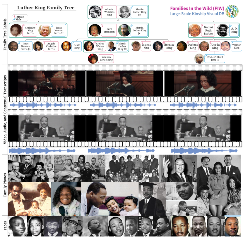
Figure 1: Sample family of FIW MM. Top-to-bottom: family-tree labels show faces of members in the immediate family, with subjects of the same generations in the same row; videos, audio, and contextual exemplify sample video pairs of Dr. King Jr. and his daughter Andrea with tracklets of faces in the visual domain and audio data aligned frame-by-frame; randomly selected  family photos that contain Dr. Luther King Jr. (note, cropped to fit); faces of Dr. King Jr. from adolescence-to-adulthood. Multiple faces are available for most subjects. Best viewed electronically.

The proposed shows that MM improves the SOTA in kinship recognition.  Our contributions to the FR, biometric, anthropology, and MM communities are three-fold.

• Built MM database: extended FIW with MM data (i.e., video tracks, speech segments, and text transcripts) via an automatic labeling scheme – $>$600 audiovisual samples for $\geq$ two members of 200 FIW families).  We reorganized FIW MM for the added metadata and paired data at the subject and instance levels, respectively. 

• Created protocols and benchmarks: a new paradigm for kinship recognition using MM data. Specifically, the updated experiments to template-based, as there is  often a  variable number of samples per subject in real-world settings. We are the first to do kinship recognition with multimodal template-based data with family tree labels. 

• Proved the advantage of MM: we show an increase in system performance from still-images  to still-images and videos, and then, again, with speech signals added – a clear benefit of each added modality is shown. Our analysis highlights the shortcomings of the different media types for future work to address.

This work will attract more scholars to kin-based problems using MM. FIW MM will be accessible online.

Table I: Commonly used acronyms and variables.

	FID	Family ID
	MID	Member ID
	PID	Picture ID
DB Terms	VID	Video ID
	BB	brother-brother
	SS	sister-sister
	SIBS	brother-sister
	FD	father-daughter
	FS	father-son
	MD	mother-daughter
	MS	mother-son
	GFD	grandfather-granddaughter
	GFS	grandfather-grandson
	GMD	grandmother-granddaughter
	GMS	grandmother-grandson
	GGFD	great
	GGFS	great
	GGFD	great
Pair-types	GGMS	great
	FMD	father/mother-daughter
Tri-Pairs	FMS	father/mother-son
	CMC	Cumulative matching characteristic
	DET	Detection error trade-off
	FAR	False-acceptance rate
	ROC	Receiver operating characteristic
Metrics	TAR	True-acceptance rate
	FR	Facial recognition
	SVM	Support vector machine
Task / solution	TA	Template Adaptation
	$P$	Probe
	$G$	Search gallery
	$X$	Template
	$x$	Media sample
	$x^{+}$	Encoded positive sample
	$x^{-}$	Encoded negative sample
	$z$	Encoded media sample
	$N_{+}$	No. positive templates
Experimental	$N_{-}$	No. negative templates

2 Related Works

Attempts to recognize kinship in media began with domesticated animals (e.g., dogs [hepper1994long] and sheep [POINDRON200799, poindron2007maternal]), as many species recognize their kin through various signals (e.g., touch, smell, visual, and acoustics). From this, we hypothesized that information in MM, besides image-level facial features, can be used to detect kinship in humans better.  Hence, knowledge extracted from imagery lacks much information. Modeling more complex signals (e.g., face dynamics and speech in videos) attribute inheritable traits (e.g., expressions, mannerisms, and accents). Nonetheless, getting MM is expensive. We propose a method to collect data and show recognition improvements with MM.

We next review existing work in visual kinship recognition and then research advances audiovisual  data for FR.

2.1 Kinship recognition

Computer vision researchers began using faces to recognize kinship about a decade ago, where Feng et al. proposed to model the geometry, color, and low-level visual descriptors extracted from faces to discriminate between KIN and NON-KIN [fang2010towards]. Others then formulated the problem as various paradigms (e.g., transfer subspace learning [Xia201144, xia2012understanding], 3D face modeling [vijayan2011twins], low-level feature descriptions [zhou2011kinship], sparse encoding [fang2013kinship], metric learning [lu2014neighborhood], tri-subject verification [qin2015tri], adversarial learning [zhang2020advkin], ensemble learning [wang2020kinship], video understanding [zhang2014talking, sun2018video, georgopoulos2020investigating], and, most recently, video-audio understanding [wu2019audio]). A common factor is the attempt to improve discriminatory power for classifying face pairs as KIN or NON-KIN; another commonality was the limited sample size and, thus, unrealistic experimental settings.

Robinson et al. introduced a large-scale image dataset to recognize families in still-imagery called FIW [robinson2016families, robinson2018visual]. FIW has 1,000 families with an average of 13 family photos, five  family members, and 26 faces. It came with benchmarks for 11 pairwise types, with the top performance of the baselines being a fine-tuned CNNs (i.e., SphereFace [liu2017sphereface] and Center-loss [wen2016discriminative]). This was the beginning of big data in kin-based vision tasks– deep learning could then be used to overcome observed failure cases [wang2017kinship, wu2018kinship]. Furthermore, new applications such as child appearance prediction [ghatas2020gankin, gao2019will],  and familial privacy protection [mingaaai2020] were made  recently.

Nowadays, FIW continues to challenge researchers with various views of image-based tasks. A myriad of methods showed the ability of machinery to use still-images to find kinship in a pair or group of subjects. Nonetheless, only so much information can be extracted from still-images. The dynamics of faces in video data (e.g., mannerisms expressed across frames) have other information, and audio and text transcripts (i.e., contextual data describing the speech and other sounds) can widen the range of cues we model to discriminate between relatives and non-relatives. We propose the first large-scale multimedia dataset for kinship recognition. Specifically, we used the familial data of the FIW image database to build upon the existing resource [robinson2016families, robinson2018visual], using the still-images of FIW and adding video, audio, audiovisual, and text data of subjects. Note that the difference between the video and audio compared to the audiovisual  is that the former two are single modality and the latter has multiple modalities– audiovisual  clips have talking-face tracks  aligned with the speech signal. After its predecessor, the  database was dubbed FIW MM. En route to bridging research and reality,  we follow the protocols of FIW [robinson2020recognizing], but now can be template-based (i.e., per National Institute of Standards and Technology (NIST) in [maze2018iarpa]). Figure 1 depicts a sample family with MM for MLK and his daughter. 

An annual data challenge that was based on FIW intended to attract more attention by supplying more structure and incentives for researchers to work on kin-based visual recognition.  Namely, the Recognizing Families In the Wild (RFIW) series,  which has been held annually since 2017 [robinson2017recognizing], and with the latest in 2020 [robinson2020face]. There have been many great attempts on the still-images as a result [KinNet, AdvNet]. Recent surveys [qin2019literature], tutorials [robinson2018recognize], and challenges [lu2014kinship, lu2015fg, wu2016kinship, robinson2020recognizing] elaborate on RFIW and the various submissions.

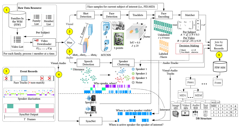
Figure 2: Our automated labeling framework. We extended a subset of families from FIW with $N$ YouTube videos for $M$ subjects (i.e., $M>1$). Upon selecting the candidates, we generated and processed a list of videos per family, processing a single subject (i.e., video-by-video) per iteration (1). First, we processed visual data: video shot detection (i.e., C shots per video), detected face-tracks with $J$ samples per shot (i.e., $J<26$ faces): tracks continued for as many as 25 frames or if the IoU ¡ 0.3 for neighboring bounding boxes. Next, ArcFace encoded all faces (i.e., the $J$ unlabeled face-tracks and the $I$ labeled faces). Then, we compared labeled and unlabeled faces via cosine similarity, yielding a score-matrix ($J\times I$): fusing the score-matrix to a single decision (i.e., Match or Non-Match) was done as follows: (i) the mean score of each frame across labeled samples produced a score vector of the size $J$; (ii) scores below the threshold (i.e., 0.3) were marked Non-Match; (iii) the 25-percentile of the samples marked as Match represented the final, fused score; (iv) the fused score was compared to a threshold of 0.25 and, if greater than, the face-track was assumed to Match the current subject of interest, which also represented in an event record to indicate frames with tracks that Match (2). Returning to the Mux and following the Audio branch: we transformed audio signals to speech utterances, clustered speaker IDs into $K$ clusters for $K$ subjects, and recorded them as events (3). Returning to signal before Mux (i.e., before splitting the visual and audio modalities), we used the audiovisual data to detect frames with the active speaker visually displayed, which we also recorded as events (4). Next, the event records of size $T$ from steps 2-4 allowed us to produce a final record based on the agreement in records: we compared the event records to filter the samples of interest via logical AND (5). Finally, we stored the MM data in the FIW MM database (6). Details for each step are in Section 3.2. Best to view electronically.

2.2 Audiovisual data

The big archetypal data  used for audiovisual  identification problems are Voxceleb [nagrani2017voxceleb] and Voxceleb2 [chung2018voxceleb2]. Like FIW MM, the datasets were acquired by extending image collections (i.e., Voxceleb and Voxceleb2 extended of the VGGFace [Parkhi15] and VGGFace2 [Cao18], respectively). Currently, the primary usage of Voxceleb is in speaker-based tasks, such as using the audiovisual  data to detect and classify the speaker by the who and the when [ephrat2018looking]. Other speaker-centric  problems have been proposed using the Voxceleb collections, like to enhance speech signals [afouras2018conversation], to detect when and where the speaking face is visible [Chung17a], and when the audio and mouth motions infer the lips and sound are in sync [Afouras18b]. Nonetheless, the lip-reading task predates the larger Voxceleb with older lip-reading datasets [Chung16, Chung17].

It is worth highlighting that these audiovisual  databases were instrumental in applied research as well (e.g., generating talking-faces [Chung17b], where the input is a still-image face and a stream of audio, and the output frames  mocking the audio with the faces as if the input face was regurgitating the audio clip). In [wiles2018x2face], face frames were generated from a still-image and audio clip, with pose information added as a control signal for the synthesized output. Furthermore, Voxceleb predicted emotion labels via its signals to automatically infer ground-truth [Albanie18].

Minimal  attempts to  recognize kinship in audiovisual data have been made.  Most relevant was in [wu2019audio], where the authors collected  400 pairs. Wu et al. certainly proved the core hypothesis of this work– multimedia can enhance our ability to automatically detect kinship in humans– as was clearly shown in their work [wu2019audio]. However, the sample size was limited in the number of pairs and the types of labels, as there is no family tree structure nor multiple samples per member (i.e., age-varying), as is the case in our much more extensive and comprehensive FIW MM.

3 The FIW-MM Database

FIW MM extended the existing paired faces  of FIW via  an automated labeling pipeline that allowed the proposed data  to be acquired with no financial cost and minimal human input (Figure 2). Specifically, FIW allowed us to find who, when, and where a family member appeared in the video. We chose 200 (of the  1,000) FIW families with  2-5 members in 1-3 YouTube videos. Hence, FIW MM consists of  550 subjects in 660 videos. We obtained three types of data per subject per video: (1)  non-speaking face tracks (i.e.,  visual only), (2)  speech segments (i.e.,  audio only), and (3)  face tracks of the  speaker (i.e.,  audiovisual).  Timestamps were  set for the start and end frames, along with the bounding box information for the face tracks.  In this way,  overlap in samples was  identifiable.

Let us next cover the data specifications, along with a detailed description of our automatic labeling pipeline.

3.1 Specifications

The goal was to extend FIW in the number of samples and the types of media. Plus, improved experimental protocols. Recalling that FIW supplies name metadata and face images for multiple members of 1,000 families [robinson2018recognize], we used this from the 200 families. For quick reference, common acronyms and symbols are in Table I.

Table II: Database statistics. Types are split based on the span in the generation of the relationship.

	1st Generation			2nd Generation				3rd Generation				4th Generation
	BB	SS	SIBS	FD	FS	MD	MS	GFD	GFS	GMD	GMS	GGFD	GGFS	GGMD	GGMS	Total
# Subjects	883	824	1,542	1,914	1,954	1,892	2,041	426	463	483	526	39	30	45	37	13,099
# Families	345	334	472	666	676	665	670	154	174	178	191	9	10	11	10	953
# Still-images	40,386	31,315	46,188	83,157	89,157	57,494	63,116	8,007	6,775	6,373	6,686	408	410	798	797	441,067
# Clips	123	79	81	155	134	147	138	16	18	25	15	2	4	0	0	937
# Pairs	641	621	1,138	1,151	1,253	1,177	1,207	263	280	292	324	28	18	36	28	8,457

Following the  convention of the original FIW [robinson2016families], the indices of the topmost level of the database were unique Family IDs, which have $M$ Member IDs for $M$ family members. Each FID is represented by a relationship matrix of size $M$ (i.e., a row and a column added per MIDs), along with the gender information for each member. Thus, FIW is organized with 1,000 folders (i.e., one per FID, F0001-F1000), each with a relationship matrix that relates the $M$ MIDs that have face data stored in subfolders (e.g., family F0009 has $M=7$,  meaning the folder contains 7 MID folders, MID1, …, MID7). The same scheme is adopted for FIW MM, with the difference being that the MID folders now have a folder per media type (i.e., subdirectory images added to MID folder for which existing face images are now stored). Besides, folders for other media types were added.

3.2 Data pipeline

Inspired by earlier work, such as FIW [robinson2018visual] (i.e., labeling families) and VoxCeleb [nagrani2017voxceleb] (i.e., labeling audiovisual  data), we formed the basis for our pipeline. From this, three modality-specific branches processed the data independently. Specifically, the branches process the video, audio, and audiovisual  modalities. Furthermore, branch-specific events are recorded by the frame number and used to summarize instances that are propagated between records. 

The following subsections are numbered according to the yellow circle callouts in Figure 2.

Step 1.  Raw data resource. A single-family  with at least two members on YouTube  was selected (i.e., families with only one member with MM would be useless). Video URLs were queried per unique Video IDs (i.e., $v_{1},\dots,v_{N}$ for $N$ videos). The videos were either interview-style (e.g., with only a news anchor in a plain room answering scripted questions) or face-time clips (i.e., self-recordings with the subject speaking directly to the camera). Also, the ethnicity for subjects was  manually collected.

We used Pypi’s youtube-dl to download YouTube videos by URL: each renamed to its VID and stored as an  MKV file, along with TXT with captions when available. The raw data consists of the original MKV for the audiovisual  branch, audio-only (WAV), and visual-only  (MP4) extracted with FFmpeg  assuming 25 FPS.

Table III: Task-specific counts. Per task (i.e., verification in top row and identification bottom three), individuals (I), families (F), images (S), video-clips (V), audio snippets (A), audio snippets (VA) in the set of probes (P), gallery (G), and total (T).

	Train					Val					Test
	I	F	S	V	A	I	F	S	V	A	I	F	S	V	A
T	2,976	571	16,464	290	7,217	955	190	5,458	72	3,308	972	192	5,231	91	1,775
P	571	571	3,039	47	1,843	190	190	1,334	16	789	192	192	993	23	876
G	2,475	571	13,571	244	5,581	791	190	4,538	56	2,519	800	192	4,705	69	899
T	3,046	571	16,610	291	7,424	981	190	5,872	72	3,308	992	192	5,698	92	1,775

Step 2.  Event records. Before branching, blank (sequential) tabular records were instantiated for the duration of the video– one record per branch  denoted 3-5 (i.e., audio, visual, and audiovisual  event records). These are later compared to share knowledge between the branches to help filter out samples of the subject of interest. In essence, the mutual information across records at a given instance (i.e., frame-step) is  used to imply matches, contradictions, and non-matches across modalities (i.e., a means to propagate labels across modalities). The usage of set theory helps to both confirm matches and filter out non-matches. Although unique to our problem, the concept of using logic across events to parse videos has been done (e.g., [haq2019movie]); however, opposed to high-level semantics like types of objects, we care about the more straightforward tasks of a  face or no face, speech or not, visible or unseen, and then the same or different subject. Furthermore, doing this increases the random chance by adding more evidence across records. 

Specifically, and for one video simultaneously, the  three-event  records are instantiated with zero event entries. Then, events of each branch are recorded. The type of event is  later described for each branch: like branch 3, visual branch, the events are face tracks that is a match with BB coordinates recorded for all frames of the shot; the audio branch consists of instances that each of the $k$ speakers pronounces  utterances; the record for the audiovisual  branch is  when the speaker is visible in the current frame. Then, by propagating the frame number that the subject of interest appears, the other audio instances with the same speaker and the frames where the speaker is  visible can be inferred by finding intersecting events between the three records.

Step 3.  Visual branch. A video was first parsed into scenes by using two global measures and with the assumption that, statistically, neighboring frames of the same shot will match as close as 90% when comparing HSV (i.e., color) and local binary patterns [ahonen2006face] (i.e., texture) features. The features were extracted and used to parameterize two probabilistic representations per frame (i.e., one per feature). Then, neighboring frames were measured via KL-Divergence and compared with a threshold of 0.1 [sanchez2017multimedia]. A pair of frames that scored below the threshold were assumed to be shot boundary frames for $V$ videos of size $T\text{,}$ i.e., $v_{t}\in\{1,2,\dots,C\}$  represents all shots detected in the $i$-th video. The first, last,  and the frame closest to the centroid (i.e., in color and texture) were used as the shot: the three frames were run through an  MTCNN face detector [zhang2016joint], and for those without at least one face detection were assumed face-less scenes. Otherwise, the clips with face detections had as many as five more frames sampled and passed to the face detector, and then all faces were encoded and compared to the faces for members of the respective family in FIW. Events were then recorded for the face tracks that matched the subject of interest. Note that this could to quickly drop unwanted data  and reduce noise in events assumed by the other branches.

Faces were encoded with ArcFace via the architecture, settings, and matcher of [deng2019arcface]. Specifically,

$$d_{boolean}({x}_{i},{x}_{j})=d({x}_{i},{x}_{j})\leq\theta,$$ (1)

where the matcher $d_{boolean}$ compared the $i^{th}$-to-$j^{th}$  face encoding of FIW [LFWTech]. Hence, $d_{boolean}$ is the decision boundary in score space– if threshold $\theta$ is satisfied, assume match; else, non-match. Note that it is currently assumed that $i$ and $j$ are from different sets (i.e., with $J$ labeled samples from FIW and $I$ face detections from newly collected). The matcher in Eq 1 was set as cosine similarity the closeness of the L2 normalized [wang2017normface] features  by $d_{boolean}({x}_{i},{x}_{j})=1-d({x}_{i},{x}_{j})=\frac{z_{i}\cdot z_{j}}{||z_{i}||_{2}||z_{j}||_{2}}>\theta$,  where $z$ represents media encoding. We set $\theta=0.2$ manually for a high recall. This process - including the usage of ArcFace to encode faces - is the matcher used throughout.

In the end, scenes having the subject of interest had all its frames processed by the MTCNN– the bounding box coordinates, fiducials (i.e., 5 points), and confidence scores were recorded for each step. We then processed the BB coordinates to ensure continuity, dropping those without it: the ROI was set on the prior face location, and the IoU was calculated frame-by-frame, which had to surpass a threshold of 0.3. Finally, up to 25 (i.e., $J$) faces were sampled per track  and passed to $d_{boolean}$  with each of the $I$ labeled faces (i.e., producing $J\times I$ score matrix). The mean across $I$ samples produced a single score per the $J$ faces, at which point the value at the 25-percentile was compared to a higher threshold of $\theta=0.25$. Note, the fusion of scores was done to both consider all the existing labeled faces equally  while avoiding much weight on any of the few (of $J$) potentially low-quality faces. This step alone yielded many face tracks of type match with high  confidence.

Step 4.  Audio branch. Audio signals were  extracted from the videos and saved as high-quality WAV files. For the entire audio clip,  we did speaker diarization– the process of detecting utterances of speech (i.e., the when), to then form $K$ clusters for $K$ speakers (i.e., the who). Note that the clusters are arbitrarily assigned IDs per video. In the end, a speech detector determined the when, and clusters determined the number of speakers and, thus, the speech segments from the who. The utterance detector used was SpeechRecognizer, and clusters were based on models from [chung2020in].

Step 5.  Audiovisual  branch. The aim was  to detect when the speaker is in the field of view. Thus, the purpose was to find the frames for which the face and speech were aligned. An intuitive way would be to relate the faces detected, lip motions, and audio– which is at the core of many speaker ID methods in MM [zhu2020deep]. For this, videos were processed using SyncNet [Chung16a]), pre-trained from [li2017targeting]. The output was  the BB at frames for which the audio aligned to that face.

The faces tracks belonging to the subject of interest were found and used to record events.  Furthermore, these events, compared with the audio events, allowed the cluster holding all speech utterances of the subject of interest formed at Step 4 to be figured out.

Step 6.  Outputs and DB structure. The face tracks, audio segments, and audiovisual  tracks of the subject of interest are output and retractable via the final event record (i.e., the three records merged with only positive instances). Thus, the  overlap between audio and audiovisual  infers which cluster of audio segments belongs to the respective active speaker, while the processing of the visual and comparison to the original FIW allowed for the subject of interest to match up with the active speaker. Any overlap in the data found in the visual branch or audio branch versus the audiovisual  was  removed as duplicated instances. The face tracks, speech segments, and clips with aligned audiovisual  were added to the folder named after media type in the MID folders, along with the final event record (i.e., the event record is enough to parse raw data). Then, the database is $N$ FID folders with $M$ MID folders  and a relationship matrix. 

Table IV: True Acceptance Rate (TAR) (%) at specific False Acceptance Rate (FAR). Scores are for template-based settings: Image only (left column), Image + Video (middle), and Image + Video + Audio (right). Higher is better.

FAR	BB			SS			SIBS			FD			FS			MD			MS			Avg.
0.5	97.8	97.8	98.2	91.5	92.3	92.7	91.7	90.8	91.5	79.8	77.8	79.9	85.3	85.3	87.1	90.6	88.8	91.4	81.3	82.6	85.2	88.3	87.9	89.8
0.3	94.1	94.1	95.3	88.0	87.2	90.1	82.9	83.9	85.7	63.5	66.5	69.3	77.1	79.1	81.5	82.4	82.3	85.0	68.9	70.1	73.4	79.6	80.4	81.6
0.1	88.1	87.4	88.4	76.1	76.1	79.1	68.7	68.2	70.2	34.5	36.9	42.9	54.3	54.3	58.2	62.2	63.1	69.4	46.1	46.5	50.1	61.4	61.8	64.9
0.01	70.4	70.4	73.6	54.7	55.6	59.9	44.2	46.1	52.4	5.9	7.9	12.9	23.6	24.0	32.1	28.3	31.3	40.6	11.6	13.3	21.0	34.1	35.5	41.1
0.001	54.8	57.0	61.1	47.9	48.7	52.4	29.5	29.0	33.7	2.0	2.5	7.7	9.3	10.9	14.1	14.2	14.6	18.5	3.3	4.6	7.8	23.0	23.9	30.1

4 Problem Statements

Following the recent RFIW data challenge [robinson2020recognizing], we benchmark two kin-based tasks: kinship verification and search & retrieval of family members.  In RFIW  and the contemporary works in kinship recognition, protocols are image-based,  i.e., unimodal, single-shot experiments. By contrast, FIW MM supports multimodal,  with added samples and media types (Table II). Provided the MM, protocols are template-based, like with IJB-A [maze2018iarpa].

Kinship verification has been the primary focus of  experiments. More recently, the emergence of the more challenging  but more practical  task of searching for missing family members was supported [robinson2020recognizing]. We benchmark FIW MM for both tasks. With the difference being the template-based [maze2018iarpa]– approaching settings of operational use-cases.

We next provide details for template-based recognition tasks. Then, we describe the tasks:  first kinship verification and  then search & retrieval of family members. The paragraph structure stays consistent:  task overview, data splits and settings, and task-specific metrics.

4.1 Definitions and protocols

Template $X$ holds all media for a subject (i.e., images, videos, audio clips).  Hence, $X$ consists of samples $x$, with a total of $N$ templates for the $n^{th}$ independent piece of media $x_{n}$, with a size of the sum of all data samples, $N=N_{I}+N_{V}+N_{A}$. We stored features for all samples. Now, the templates include feature vectors, i.e., $\mathcal{F}(x)=z$, where $\mathcal{F}$ maps face to the feature space via $\mathcal{F}(x)\in\mathbb{R}^{\mathrm{d}}$, and with $d$ being the size of the vector.  We set a subject-specific template as  probe $P$ (i.e., query) or reference $Q$ (i.e., hypothesis). For 1:$N$, known subjects were from a known family, and  templates enrolled in gallery $G$. Then, at inference, the goal was to match an unseen probe $P$ with $G$, where $|G|$ refers to the  number of templates enrolled in the gallery.  As mentioned later,  for 1:1-based evaluation,  we assume $|G|=1$ (i.e., compared the template for $P$ with the template of $G$ to decide whether the pair is KIN or NON-KIN). For $|G|>1$,  the one-to-many 1:$N$ search & retrieval task outputs ranked lists of template IDs sorted by the likelihood of being a blood relative (e.g., if $|G|=10$, then template of $P$ will compare with the ten  templates of $G$, to generate a list of indices [1, 10] ordered by score compared with probe $P$). 

As mentioned, we treat  an audio segment (i.e., a clip of a  subject speaking without interruptions or significant  pauses) as a single piece of media $x\text{,}$ which is fused to a single representation by averaging across frames. Note that a video may consist of several disjoint tracks,  visual, audio, and audiovisual  (i.e., aligned). Thus, there are many independent media samples for both the visual and audio modalities. Again, this is the set of media making up template $X$ per subject, which contains  various media samples $x$, such that the $j^{th}$ subject can be represented by $k$ media samples as follows: $X_{j}={\mathcal{F}_{t}(x_{1}),\mathcal{F}_{t}(x_{2}),\dots,\mathcal{F}_{t}(x_{k})}$, where $t$ corresponds to the media type and, hence, the corresponding encoder. From this, $|X_{j}|$ is the total number of features  for subject $j$. The gallery $G$ consists of a set of subjects by $G=\{(X_{1},y_{1})^{l},(X_{2},y_{2})^{l},\dots,(X_{n},y_{n})^{l}\}$, where $y$ are identity labels for each of the $N$ subjects, and $l\in\{1,2,\dots L\}$ are ground-truth for $L$ families. Each tuple also contains  a tag representing the set of $L$ families (i.e., $(X_{j},y_{j})^{l}$), where $l\in\{1,2,\dots,L\}$. Further partitioning of the data is done per the  requirements of a task. For instance, for the verification, the $i^{th}$ pair of tuples from the same family $\mathbb{P}_{m}=((X_{i},y_{i})\bigcap(X_{j},y_{j}))$, where $i\neq j$, inherit labels KIN (i.e., match) and relationship type.

Each task consists of a ($\approx$60%) train, ($\approx$20%) validation, and ($\approx$20%) test set. These sets are disjoint in family and subject IDs– sets were generated by splitting family labels, with partitioning that remained constant for all tasks.

4.2 Kinship verification

Kinship verification is the simplest  of tasks in this challenging and complex problem space.  Hence, this one-to-one paradigm is the main view vision researchers have tackled. The task is to figure out whether a face pair  are blood relatives (i.e., true kin or match). This face-based problem inherits all the challenges of conventional FR,  such as variations in lighting, pose, and occlusion (e.g., sunglasses or beards). Additionally, several challenges specific to kin-based FR are posed by age variations, face pairs that contradict directional relationships (e.g., grandparent-grandchild, where the face image of the grandfather was from a younger age and that of the grandchild was older), bias across  subgroups like in FR [robinson2020face] but amplified for the kin-based data. 

The most fundamental question asked in kinship verification  and re-asked in all other kinship discrimination tasks  is whether a face pair is related. Therefore, kinship verification is the  boolean classification of pairs (i.e., ${y}\in\{\emph{KIN}\bigcup\emph{NON-KIN}\}$). Typically, knowledge of the relationship type is assumed. Thus, supplied the output of the model for a given pair is KIN, then the specific type is implied. Future efforts could incorporate relationship-type signals to advance capabilities of kinship detection systems; however, and as stated upfront, verification provides the simplest of all the benchmarks and, up until now, is the most popular [robinson2020recognizing].

4.2.1 Data splits and settings

Conventionally, a query consists of a single face image $x_{1}$ paired with a second face image $x_{2}$ (i.e., a one-shot, boolean classification problem with labels $y\in\{\text{KIN},\text{NON-KIN}\}$). Put formally, given a set of face-pairs $(x_{1},x_{2})_{s}^{l}$, where the number of sample pairs $s\in\{1,2,\dots,S\}$ of relationship-type (e.g., mother-son). A set of pair-lists $\mathbb{P}=\{[(x_{1},x_{2})_{1}^{l}]_{\mathbbm{1}},[(x_{1},x_{2})_{2}^{l}]_{\mathbbm{1}},\dots,[(x_{1},x_{2})_{S}^{l}]_{\mathbbm{1}}\}$ for the $L$ types, and with the label determined by the indicator function $\mathbbm{1}$ for a single pair $\mathbb{P}_{s}\rightarrow\{0,1\}$, i.e.,

$$\mathbbm{1}(\mathbb{P}_{s})=\begin{cases}0&\hskip 14.22636pt\emph{NON-KIN}\\ 1&\hskip 14.22636pt\emph{KIN}\\ \end{cases}.$$ (2)

Note, a $\mathbb{P}_{s}$ consists of a pair of templates and, thus, the task is to decide whether the media of the templates provide evidence that the two persons are blood relatives; notice Eq. (2) is the template matcher defined in Eq. (1).

Table V: Identification results for Image, Image + Video, and Image + Video + Audio. Specifically, accuracy as a function of rank and mAP scores. The higher, the better.

		Rank
Modality	Fusion	@1	@5	@10	@20	@50	mAP
Image	Mean	0.29	0.43	0.54	0.64	0.78	0.13
	Median	0.28	0.44	0.52	0.64	0.77	0.13
	Max	0.11	0.19	0.28	0.34	0.52	0.06
	TA	0.31	0.43	0.52	0.63	0.74	0.14
Image	Mean	0.30	0.44	0.52	0.64	0.77	0.14
+ Video	Median	0.28	0.44	0.50	0.63	0.76	0.14
	Max	0.13	0.21	0.26	0.30	0.44	0.06
	TA	0.34	0.46	0.55	0.68	0.75	0.16
Image	Mean	0.30	0.44	0.52	0.64	0.77	0.14
+ Video	Median	0.28	0.44	0.50	0.63	0.76	0.14
+ Audio	Max	0.13	0.21	0.26	0.30	0.44	0.06
	TA	0.56	0.59	0.63	0.74	0.78	0.24

The data can be further split by the type of relationship $l$– $L$ sets of pairs organized into $L$ independent lists, meaning $\mathbb{P}_{s}$ partitioned into $l$ disjoint sets in $\mathbb{P}_{s}^{l}$ (Table III). Specifically, pair-types are brother-brother (BB), sister-sister (SS), or brother-sister (SIBS) of mixed-sex; father-daughter (FD), father-son (FS), mother-daughter (MD), or mother-son (MS); grandfather-granddaughter (GFD), grandfather-grandson (GFS), grandmother-granddaughter (GMD), or grandmother-grandson (GMS); four great grandparent types as well. Hence, $l\in L\rightarrow\{BB,SS,\dots,GMGD,GMGS\}$ with $L=11$. Statistics for all relationship types are listed in Table II, with the lists of grandparent-grandchild and great-grandparent omitted from the  verification task due to insufficient sample counts (i.e., $L=7$).

As described, FIW MM is organized as templates with many samples from various modalities (i.e., still-face, face tracks,  audio, and transcripts (contextual)). Specifically, true IDs $y$ are paired with a template of all media available for the respective subject. In contrast with conventional kinship recognition, where one image is compared to another, the 1:1 paradigm is template-based (i.e., one template compared to another). Then, a template pair $\mathbb{P}_{s}^{l}=((X_{i},y_{i}),(X_{j},y_{j}))$ is of different subjects (i.e., $X_{i}$ and $X_{j}$, where $i\neq j$).

4.2.2 Metrics

det curves and the average verification accuracy measured performances in verification, along with the TAR scores at specific values of FAR  (Table IV).

det curves show error rates for binary classification systems, plotting the false-negative rate (FNR) as a function of FAR. Type II error FNR contributes to the Type I error fpr, revealing the imposter accepted:

$$\text{FAR}=\text{FPR}=\frac{\text{FP}}{{N^{-}}}=\frac{{FP}}{\text{FP}+\text{TN}},$$

where the number of negatives is $N^{-}$. The geometric relationships of the metrics related to the score distributions and the choice in threshold show the trade-offs in error rates (i.e., Type I versus Type II error):

$$\text{FNR}=\frac{\text{FN}}{{N^{+}}}=\frac{{FN}}{\text{FN}+\text{TP}}.$$

Finally, $\acs{tar}+\acs{fnr}=1$; therefore, $\acs{tar}=1-\acs{fnr}$. 

In summary, various attempts were made for both genuine and imposter pairs, and the scores were saved. Then, by changing the threshold that converts the score to a decision, we could visualize the trade-offs between the different error types (i.e., a lower threshold means fewer rejections of genuine pairs  but more accepting of imposter pairs). Thus, the performance of the system is highly dependent on a choice in the  threshold, which is the reason DET curves are used in biometrics to see these trade-offs in binary problems.

Figure 3: Results for fusing early (i.e., feature fusion (FF)) and late (i.e., score fusion (SF)). Still-images $S\text{,}$ video clips $V\text{,}$ and audio segments $A\text{,}$ with images and video $S+V$ and images, audio, and video $S+V+A\text{.}$ Both tasks gain from early fusion: the DET curve (top) summarizes the verification task by plotting FNR versus FPR (i.e., lower is better); search & retrieval shows a CMC curve (bottom)– accuracy across ranks (i.e., higher is better).

4.3 Search & retrieval (missing family member)

Kinship identification is organized as a 1:N search and retrieval task, with each subject having one-to-many media samples. Thus, we imitate template-based evaluation protocols [maze2018iarpa]. Furthermore, the goal is to find relatives of search subjects (i.e., probes) in a search pool (i.e., gallery).

4.3.1 Data splits and settings

A gallery $G=\{g_{i}\},(i=1,...,N)$ is queried by a set of probes $P=\{p_{j}\},(j=1,...,M)$ for search and retrieval, where $g_{i}$ is the $i^{th}$ template in $G$ and $p_{j}$ is the template of the $j^{th}$ query subject. As mentioned, a template consists of samples of various modalities. Given a template of MM, various schemes were applied to integrate the identity information from all media components of $P\text{.}$

4.3.2 Metrics

Scores of $N$ missing children are calculated as

$$AP(l)=\frac{1}{P_{L}}\sum^{P_{L}}_{tp=1}Prec(tp)=\frac{1}{P_{L}}\sum^{P_{L}}_{tp=1}\frac{tp}{rank(tp)},$$

where average precision (AP) is a function of family $l\in L$ (i.e., $|L|={P_{L}}$) for a given true-positive rate (TPR). All AP scores are averaged to find the mean AP (i.e., mAP):

$$mAP=\frac{1}{N}\sum^{N}_{l=1}AP(l).$$

Also, Cumulative Matching Characteristic (CMC) curves as a function of rank enable for analysis between different attempts [decann2013relating], along with the accuracy at rank 1, 5, and 10.

Our choice in metrics is typical for judging the  ranking capabilities of classification (or identification) systems. Like the DET assesses the 1:1 case of verification, CMC measures the 1:$m$ performance in ranking-based problems.

5 Benchmarks

5.1 Methodology

The problems of FIW MM have various views– multi-source and multimodal.  The former varies in samples and treats  the different media types  independently until the matching function outputs scores (i.e., late-fusion). The latter demands a method for the  early fusion (e.g., feature-level), enhancing  performance by using informative samples while ignoring noisy and less discriminating samples. We next describe the modality-specific features (i.e., encoding different media types)  and methods of fusion.

5.1.1 Visual features

We represented each visual media sample  as the encoding from Arcface CNN [deng2019arcface] (i.e., ResNet-34). MS1M [guo2016ms] was the train set, which had $\approx$5.8M faces for 85,000 subjects. Faces were detected with MTCNN [zhang2016joint],  returning the five facial landmarks (i.e., two eyes, nose, both corners of the mouth). Then, faces were cropped and aligned using a similarity transformation on the five points with references set by the eye locations. Once cropped, we resized the faces  to 96$\times$112. The RGB (i.e., pixel values of [0, 255]) were center about 0 (i.e., subtracting 127.5) and then standardized (i.e., divided by 128). We passed images through a CNN to map to features–  all features  were later L2 normalized [wang2017normface]. During training, the batch size  was 200, and an  SGD optimizer with a momentum of  0.9, weight decay 5e-4, and learning rate starting at 0.1 and decreasing 10$\times$ twice, both times when the error leveled. We followed the settings of  the SOTA Arcface– a popular choice for an off-the-shelf choice for FR technology and applications.

We processed  both images and videos as described, with the mapping from image-space to feature-space denoted by $\mathcal{F}(x)\in\mathbb{R}^{\mathrm{d}}$, where the dimension $\mathrm{d}=512$ for ArcFace. Face tracks from video data are fused to a single encoding by average pooling the same track features. We represent  a face track of $M$ frames as $\bar{z}=\frac{1}{M}\sum_{x}\mathcal{F}(x)$. This reduces the effect of noisy frames  and smooths out the final representation to weigh like  all other media samples.

5.1.2 Audio features

We encoded all speech segments  with a SOTA deep learning model [chung2020in].  Specifically, we trained SqueezeNet [iandola2016squeezenet], a 34-layer ResNet [he2016deep], with an angular prototypical loss and optimized with Adam [kingma2014adam] to transform WAV-encoded audio files to a single encoding (i.e., $f(x)=z\in\mathcal{R}^{512}$). Thus, per the  angular prototypical loss [snell2017prototypical], used alongside softmax, minimizes within-class scatter (i.e., penalty formed as the sum of Euclidean  distances from all samples of a subject from the mean centroid of the respective mini-batch). Expressly,  a support set $S$ and a query $Q$ are set in each mini-batch on a subject-by-subject basis, with $Q$ made up  of a single utterance to compare with the centroid of $S$ that consists of all other samples in the mini-batch for that class. Angular prototypical takes advantage of the perks of using centroid prototypes  while enhancing by following generalized end-to-end (GE2E) [wan2018generalized] usage of a cosine-based similarity metric. This is scale-invariant, is more robust to feature variance, and helps convergence during training [wang2017deep]. 

5.1.3 Naive fusion

We show results from various  naive fusion techniques (e.g., average pooling of features and voting of scores). To no surprise, the score-based fusion outperforms the feature-level fusion schemes. Specifically, the mean of all scores, both within a template and comparing templates, further improved by adding the other media types (Table IV).  The gain from each added modality is clear from just the naive score-fusion. Still, the naive fusion methods at the feature level are an ineffective way of combining knowledge. Provided media - media that vary  in modality, quality,  and discriminative power - a simple, unweighted average across the items of a template does not exploit all information. To better fuse the template, we adapt a model to the template to better discriminate family members. 

5.1.4 Feature fusion

ta [whitelam2017iarpa] is a form of transfer learning that fuses labeled face features  from a source domain with template-specific  Support Vector Machines trained on the target domain. We followed probe adaptation settings for kinship verification;  for identification (i.e., search & retrieval), we follow gallery adaptation settings. Regardless of the setting, the goal is to train a similarity function from a probe template $P$ to either a reference template $Q$ (i.e., similarity $s(P,Q)$) or gallery $G$ (i.e., similarity $s(P,G)$) for probe adaptation and gallery adaptation, respectively. Thus, given $P$, we train an SVM on top of its encoded media in $x^{+}$ and $x^{-}$ as the positive and negative, respectively:  for probe adaptation), the negative set is formed by sampling a single sample from all other templates to use for $P$ and $Q$; for gallery adaptation, the negatives are of templates in $G=\{X_{1},X_{2},\dots,X_{m}\}$ besides the $i^{th}$ template $X_{i}\neq X$. Either way, template adaptation (TA) allows for the early fusion of different media types with many more negative samples (i.e., $x^{+}\ll x^{-}$). The number of positive samples is minimal (i.e., $|P|<<|N|$); hence, the SVM-based modeling mitigates imbalanced data about the number of positives versus negatives. Notably, a kernel space defined by the largest margins found by SVMs handled cases with one or few samples the best. 

Finally, let $P(q)$ represent the evaluation of media features  of template $Q$ upon being trained on $P$, and vice versa for $Q(p)$ to use knowledge from both directions: 

$$s(P,Q)=\frac{1}{2}P(q)+\frac{1}{2}Q(p).$$ (3)

The similarity score is the result of the templates fused.

The benefit of SVMs is in the kernel. Specifically, the linear, max-margin modeling scheme of a vanilla SVM has proven effective at separating a non-linear feature space between two classes; (i.e., $i$ and $j$, where $y_{ij}=\pm 1$ for the same ($+$) and different ($-$) classes). Thus, the implicit embedding function (i.e., kernel) $K(x_{i},x_{j},y_{ij})=\varphi(x_{i},y_{i})\varphi(x_{j},y_{j})$ projects the encoding pair to a non-linear space such that the SVM learns the best hyperplane $\mathbf{w}^{T}K(x_{i},x_{j},y_{ij})+b=0$ separating the two classes. This is done on the  training set by (1) maximizing the margin and (2) minimizing the loss– weights $\mathbf{w}$ are learned, while bias terms $b$ are set to 1 (i.e., concatenated on $\mathbf{w}$, as an added dimension). Also, $K(x_{i},x_{j},y_{ij})=\exp{\frac{||x_{i}-x_{j}||^{2}}{2\sigma^{2}}}$ for ${y_{ij}\in\{-,+\}}$ as the respective class (i.e., Gaussian RBF kernel [scholkopf2002learning] projects all features  to a higher dimension). Then, the predicted class is inferred as $\hat{y}=\mathbf{w}^{T}\varphi(x_{i})\varphi(x_{j})+b$. We used dlib’s [king2009dlib]– L2 regularized cosine-loss with class-weighted hinge-loss, i.e.,

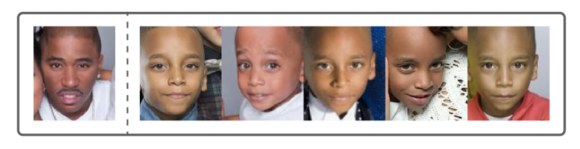
Figure 4: Template of an actual  FS pair incorrectly classified using score fusion, but correct for TA (i.e., feature fusion). Only a single face is available for the father (left), while all son instances  are at an early age (right).

$$\min_{\mathbf{w}}{\frac{1}{2}\mathbf{w}^{T}\mathbf{w}}+\lambda_{+}\sum_{i=1}^{N_{+}}\max\large{[}0,1-y_{i}\mathbf{w}^{T}f(x_{i})\large{]}^{2}$$

$$+\lambda_{-}\sum_{j=1}^{N_{-}}\max\large{[}0,1-y_{j}\mathbf{w}^{T}f(x_{j})\large{]}^{2}.$$ (4)

The protocols are set for gallery adaptation: train a similarity function $s(P,G)$ from a probe $P$ to gallery $G$. A gallery of templates $G=\{X_{1},X_{2},\dots,X_{m}\}$ are used to train the SVM (i.e., the scoring function $s(P,X_{i})$). The difference between probe adaptation and gallery adaptation is in the negative sets. Along with the sample per subject trained against for probe adaptation, global adaptation samples all other templates in $G$ as added negatives. Again, $N_{+}<<N_{-}$. The class imbalance is handled via class-weighted hinge-loss in Eq 4, with $\lambda_{+}=\lambda\frac{N_{+}+N_{-}}{2N_{+}}$, $\lambda_{-}=\lambda\frac{N_{+}+N_{-}}{2N_{-}}$, which are regularization constants inversely proportionate to class frequency. The constant $\lambda$ trades-off between the regularization and loss, which we set to 10 as in earlier work [whitelam2017iarpa].

5.1.5 Implementation

The system was implemented in Python, with CNNs for visual and audio from PyTorch’s  deep learning framework for each media encoder and SVM from LibSVM. The negative sample set was formed by randomly selecting a single instance from all other families. Hence, investigating and improving the naive means for which we pool negative samples is a promising direction for future work. With that, $N_{+}\text{ and }N_{-}$ are  set case-by-case.

5.2 Results

System performance boosted with each added modality (Fig. 3, Table IV and V). Considering the benchmarks use conventional speech and FR technology  and our hypothesis that video and audio boost  discrimination, these notable improvements would likely continue to climb supplied a more sophisticated or specific solution. It would be interesting to fuse earlier on  and train machinery jointly for audiovisual  data. From this, more complex dynamics of facial appearance, along with the corresponding speech signal, could further our knowledge and supply  insights.

There was a trend in the type of corrected samples when comparing the score-based fusion to the feature-based (i.e., TA). As shown in Figure 4, the challenge of recognizing kinship from samples of one or more members  at an early age is mitigated. TA learns to better discriminate in these conventional failure cases. Additionally, some templates with multiple instances are often better than others when comparing. Hence, TA does not simply average all instances equally, like for naive score-based fusion– fix cases with few samples are most discriminate (Fig. 5).

5.3 Discussion

The template-based protocol adds practical value by mimicking the more likely structure posed in operational settings, per NIST [maze2018iarpa]. Besides, several other factors make it a more exciting formulation and,  therefore, a higher potential for researchers to show off  their creativity. For instance, opposed to using a single sample per subject (i.e., one-shot learning), each now is represented in a set of media (i.e., a template). The question now arises  - how to best fuse knowledge and incorporate evidence from different modalities and how to best learn from all available MM data? Another consequence of using templates is that the random chance is increased from (1) the knowledge added to the  pool (or fuse) from the added modalities, and (2) the gallery size reduces from tens of thousands by nearly ten-fold. The latter is not an implication of lessor difficulty  but the byproduct of reducing bias in data [robinson2020face]. That is, opposed to having one-to-many samples per subject,  there is just one template. Mitigating specific sources of data imbalance (i.e., whether there are thirty samples or just one),  a system’s ability to recognize a particular pairing or group affects the metric evenly. In other words, a system may easily recognize a specific parent-child pair - regardless of the number of face samples and, so, the number of face pairs. Hence, the impact on the metric is proportional to the number of unique pairs.

Furthermore, for verification, we measured the impact of the different results using the significant  test. Expressly, we set the baseline image-only as the null hypothesis to compare an alternative hypothesis set as the different results (i.e., image-only, image and video, and audiovisual).  Specifically, comparing baseline to null results in a p-value of 1.000 (i.e., same results). Then, a limited improvement p-value=0.974 (i.e., the smaller, the  better) results compared to the mean of image and videos (i.e., videos add samples, but of the similar modality after averaging frames). Significant improvement in p-value=0.024 compared  with the naive fusion of MM (i.e., audio and visual), which goes to 0.000 for TA using MM. Thus, this further confirms our claim that kinship recognition systems significantly better the decisions.

6 Future Work

FIW MM pushes the bar for possibilities in automatic recognition of kinship in MM. An immediate next step for research involves gathering  experts of different domains, such as those in sequence-to-sequence modeling, whether video (i.e., visual), audio (i.e., speech), contextual (e.g., conversations and parts-of-speech), or early fusing pairs or groups. Let us next discuss a variety of ways that we foresee the data being beneficial and to form a  collaboration amongst different research communities  and beyond (i.e., although FIW-MM is for non-commercial uses, the resource has high  commercial potential and, thus, proof of principle experiments can motivate business moves). 

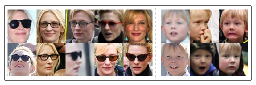
Figure 5: A MS pair incorrectly classified with late fusion but correct with early fusion (i.e., TA). The young age of the son and most faces of the mother occluded by sunglasses pose a challenge (i.e., score fusion puts equal weight on all samples, where TA learns to discriminate better). 

We expect FIW MM to bring anthropology and genealogy experts together with researchers of MM and ML to help find the hidden patterns connecting families in MM. For instance, we showed that simply  applying pre-trained models from the speech recognition domain allows for the audio signal to be incorporated for more discriminative power than visual evidence alone. Indeed, there is room to improve over the simple benchmark. Furthermore, high-level semantics (i.e., attributes) like accents, commonly used phrases, and speaker demeanor could boost the overall performance and supply insights by interpretation. Similarly, studies on familial language components and inherited changes, or even deltas across the same generation (i.e., commonalities and differences in siblings’ speech), can too be quite revealing. A similar potential exists for the videos and audiovisual data in model complexity and use-cases.

The family trees, an  abundance of data points, rich metadata for individuals,  and relationships among MM data – FIW MM could serve as a basis for group-based (i.e., social) data mining. More data can enhance or target specific nature-based studies, traditional ML-based audio, visual, and audiovisual  tasks, or even extend this dataset. Fusing audiovisual  data is an ongoing, unanswered problem [song2019review]. Note that FIW-MM in its entirety pose more problems than it solves: from the model training  to improvements made when dealing with missing or incomplete modalities, and even the data processing and data imbalance; from the underlying roots of the problem to the high-level semantics, similar to modern biometrics systems with audiovisual  data, FIW MM is an appropriate step considering the state in visual kinship recognition technology.

Another direction is fusion. We included early and late fusion by merging the media as features and scores, respectively. Scores were fused by naively averaging– ignoring the signal type  and assuming all samples should carry the same weight. Fusion can incorporate more sophisticated techniques: cross-modality, selectively choosing the best quality samples or model-based  decision trees. This concept, alone, is vastly in need of solutions– whether data fusion, where the input is clips of aligned audiovisual;  early-fusion, as we did via TA to fuse at the feature-level; or late-fusion, which we also included by naively averaging scores. Besides, meta-knowledge, like relationship types (e.g., directional relationships), genders, age, and other attributes, could indicate final decisions. Hence, there is  an abundance of fusion paradigms– none are trivial, yet most hold promise.

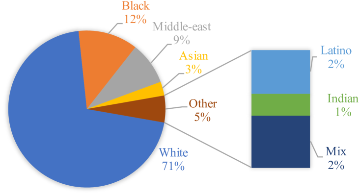
Figure 6: Ethnicity distrubution of the families in FIW. This is based on the output of pretrained ethnicity classify and, hence, is only an approximation. We used a public github, face_toolbox_keras, to acquire predicted labels.

Besides, questions concerning bias– trends as a function of gender and ethnicity; properly securing family data, addressing areas of privacy and protection. Furthermore, studies on differences between a diverse pool versus a search pool of mostly similar faces– whether it be a closer look at the effects of age for different relationship types, quantifying the similarity of specific features across different subgroups, and its effects on appearance (i.e., visual data) and speech (i.e., audio data). As has been a focus in recent works [robinson2021balancing, DBLP:journals/corr/abs-2102-02320], considerations of bias across subgroups, along with attempts to acquire a balanced set of families with respect to individual demographics .

Research topics to spawn off the proposed are vast; the specifics suggested here are limited by our imagination. We expect scholars and experts of other domains to see paradigms not mentioned here: whether it be an improved variant of adapting templates and feature fusion (e.g.,  [xiong2017good]), deciding when to fuse, a new method of integration, along with the integration details, are all open research questions.

7 Conclusion

We extended the  Families In the Wild (FIW) image dataset for kinship recognition with multimedia (MM) data– 1-3 MM samples for 2-4 members from 200 (of 1,000) families we obtained  and then renamed FIW in Multimedia (FIW MM), which is the first dataset to provide multimedia data for families in ML-related fields. In addition, we followed  new paradigms (i.e., template-based protocols) in both benchmarks (i.e., kinship verification and search & retrieval of family members)– templates mimic a realistic setting, as followed in FR-related problems, but with this a first for kin-based recognition. Our labeling pipeline uses multimodal  evidence and a simple feedback schema to use the labeled data of FIW to propagate ground truth for the added modalities. Results improve with each added media type, with the top performance obtained with an  early fusion of features of multiple modalities. FIW MM marks a significant  milestone for kin-based problems by welcoming experts of other data domains.  In addition, FIW MM supports several  recognition tasks due to its rich metadata, template-based structure,  and multiple modalities.

Joseph P Robinson B.S. in electrical & computer engineering (’14) and Ph.D. in computer engineering (’20) at Northeastern University, where he worked as part-time faculty: taught undergrads in Data Analytics (’19-’20 Best Teacher). Research is in applied machine vision, emphasizing faces, deep learning, MM, and big data. He led on TRECVid debut (MED’15, third place). Built many images and video datasets– most notably FIW. Organized & hosted several workshops and challenges (e.g., NECV17, RFIW@ACMMM17, RFIW@FG18-20, AMFG@CVPR18, FacesMM @ICME18-19), tutorials (ACM-MM18, CVPR19, FG19), PC member (e.g., CVPR, FG, MIRP, MMEDIA, AAAI, ICCV, etc.), reviewer (e.g., IEEE TBioCAS, TIP, TPAMI,etc.), and Pres. of IEEE@NEU and Rel. Officer of IEEE SAC R1 Region. Completed NSF REUs (’10 & ’11); co-op at Analogic Corp. (’12) BBN Tech. (’13); intern at MIT LL (’14), STR (’16-’17), Snap Inc. (’18), ISMConnect (’19). Currently, an AI Engineer at Vicarious Surgical (’21), working on surgical robotics.

Zaid Khan Received a B.S. in Computer engineering (’18) and is currently a Ph.D. student in Computer Engineering (’25) at Northeastern University under Dr. Yun Fu. Zaid served as the website and technical chair of RFIW 2020 held in conjunction with IEEE Conference on Facial and Gesture Recognition. His research interests lie in computer vision, with a focus on faces.

Yu Yin Received B.S. in Electrical and Information Engineering (2016) from Wuhan University of Technology, China, M.S. in Electrical and Computer Engineering (2018) at Northeastern University (NEU), Boston, MA, and is currently pursuing a Ph.D. in Computer Engineering at NEU under Dr. Yun Fu. Her research spans image processing (i.e., super-resolution, face generation), visual recognition (i.e., face recognition, pose estimation, face alignment, and emotion recognition), and biosignal processing. She served as organizing chair of RFIW Workshop Challenge @ FG’20, conference PC (e.g., AAAI & FG), and journal reviewer (e.g., IEEE Trans. on TIP & TNNLS). She interned at Zillow Group (2020).

Ming Shao Received the B.E. degree in computer science, the B.S. degree in applied mathematics, and the M.E. degree in computer science from Beihang University, Beijing, China, in 2006, 2007, and 2010, respectively. He received the Ph.D. degree in computer engineering from Northeastern University, Boston MA, 2016. He is a tenure-track Assistant Professor affiliated with College of Engineering at the University of Massachusetts Dartmouth since 2016 Fall. His current research interests include sparse modeling, low-rank matrix analysis, deep learning, and applied machine learning on social media analytics. He was the recipient of the Presidential Fellowship of State University of New York at Buffalo from 2010 to 2012, and the best paper award winner/candidate of IEEE ICDM 2011 Workshop on Large Scale Visual Analytics, and ICME 2014. He has served as the reviewers for many IEEE Transactions journals including TPAMI, TKDE, TNNLS, TIP, and TMM. He has also served on the program committee for the conferences including AAAI, IJCAI, and FG. He is the Associate Editor of SPIE Journal of Electronic Imaging, and IEEE Computational Intelligence Magazine. He is a member of IEEE.

Yun Fu (S’07-M’08-SM’11-F’19) received the B.Eng. degree in information engineering and the M.Eng. degree in pattern recognition and intelligence systems from Xi’an Jiaotong University, China, respectively, and the M.S. degree in statistics and the Ph.D. degree in electrical and computer engineering from the University of Illinois at Urbana-Champaign, respectively. He is an interdisciplinary faculty member affiliated with College of Engineering and the College of Computer and Information Science at Northeastern University since 2012. His research interests are Machine Learning, Computational Intelligence, Big Data Mining, Computer Vision, Pattern Recognition, and Cyber-Physical Systems. He has extensive publications in leading journals, books/book chapters and international conferences/workshops. He serves as associate editor, chairs, PC member and reviewer of many top journals and international conferences/workshops. He received seven Prestigious Young Investigator Awards from NAE, ONR, ARO, IEEE, INNS, UIUC, Grainger Foundation; eleven Best Paper Awards from IEEE, ACM, IAPR, SPIE, SIAM; many major Industrial Research Awards from Google, Samsung, Amazon, Konica Minolta, JP Morgan, Zebra, Adobe, and Mathworks, etc. He is currently an Associate Editor of the IEEE Transactions on Neural Networks and Leaning Systems. He is fellow of IEEE, IAPR, OSA and SPIE, a Lifetime Distinguished Member of ACM, Lifetime Member of AAAI, and Institute of Mathematical Statistics, member of Global Young Academy, INNS and Beckman Graduate Fellow during 2007-2008.

References

- [1] W. Liu, Y. Wen, Z. Yu, M. Li, B. Raj, and L. Song, “Sphereface: Deep hypersphere embedding for face recognition,” in Conference on Computer Vision and Pattern Recognition (CVPR), 2017.
- [2] I. Masi, Y. Wu, T. Hassner, and P. Natarajan, “Deep face recognition: A survey,” in 2018 31st SIBGRAPI conference on graphics, patterns and images (SIBGRAPI). IEEE, 2018, pp. 471–478.
- [3] R. Fang, K. D. Tang, N. Snavely, and T. Chen, “Towards computational models of kinship verification,” in International Conference on Image Processing (ICIP). IEEE, 2010.
- [4] J. P. Robinson, M. Shao, and Y. Fu, “To recognize families in the wild: A machine vision tutorial,” in ACM on International Conference on Multimedia (MM), 2018.
- [5] X. Qin, X. Tan, and S. Chen, “Tri-subject kinship verification: Understanding the core of a family,” IEEE Transactions on Multimedia, vol. 10, no. 17, pp. 1855–1867, 2015.
- [6] J. P. Robinson, M. Shao, and Y. Fu, “Survey on the analysis and modeling of visual kinship: A decade in the making,” IEEE Transactions on Pattern Analysis and Machine Intelligence, 2021.
- [7] J. P. Robinson, Y. Yin, Z. Khan, M. Shao, S. Xia, M. Stopa, S. Timoner, M. A. Turk, R. Chellappa, and Y. Fu, “Recognizing families in the wild (rfiw): The 4th edition,” in Conference on Automatic Face and Gesture Recognition (FG), 2020, pp. 857–862.
- [8] A. Ephrat, I. Mosseri, O. Lang, T. Dekel, K. Wilson, A. Hassidim, W. T. Freeman, and M. Rubinstein, “Looking to listen at the cocktail party: A speaker-independent audio-visual model for speech separation,” ACM Trans. Graph., vol. 37, no. 4, Jul. 2018.
- [9] A. Nagrani, J. S. Chung, and A. Zisserman, “Voxceleb: a large-scale speaker identification dataset,” in INTERSPEECH, 2017.
- [10] J. S. Chung, A. Nagrani, and A. Zisserman, “Voxceleb2: Deep speaker recognition,” in INTERSPEECH, 2018.
- [11] A. Nagrani, S. Albanie, and A. Zisserman, “Seeing voices and hearing faces: Cross-modal biometric matching,” in Conference on Computer Vision and Pattern Recognition (CVPR), 2018.
- [12] S. Albanie, A. Nagrani, A. Vedaldi, and A. Zisserman, “Emotion recognition in speech using cross-modal transfer in the wild,” in ACM on International Conference on Multimedia (MM), 2018.
- [13] M. Hao, W. Cao, Z. Liu, M. Wu, and P. Xiao, “Visual-audio emotion recognition based on multi-task and ensemble learning with multiple features,” Neurocomputing, vol. 391, pp. 42–51, 2020.
- [14] O. Wiles, A. Koepke, and A. Zisserman, “X2face: A network for controlling face generation by using images, audio, and pose codes,” in European Conference on Computer Vision (ECCV), 2018.
- [15] A. S. Koepke, O. Wiles, and A. Zisserman, “Self-supervised learning of a facial attribute embedding from video,” in British Machine Vision Conference 2018, BMVC 2018, Newcastle, UK, September 3-6, 2018. BMVA Press, 2018, p. 302. [Online]. Available: http://bmvc2018.org/contents/papers/0288.pdf
- [16] X. Song, H. Chen, Q. Wang, Y. Chen, M. Tian, and H. Tang, “A review of audio-visual fusion with machine learning,” in Journal of Physics: Conference Series, vol. 1237. IOP Publishing, 2019.
- [17] S. Petridis, Y. Wang, Z. Li, and M. Pantic, “End-to-end audiovisual fusion with lstms,” in Proc. The 14th International Conference on Auditory-Visual Speech Processing, pp. 36–40.
- [18] J. P. Robinson, M. Shao, Y. Wu, and Y. Fu, “Families in the wild (FIW): Large-scale kinship image database and benchmarks,” in ACM on International Conference on Multimedia (MM), 2016.
- [19] P. G. Hepper, “Long-term retention of kinship recognition established during infancy in the domestic dog,” Behavioural processes, vol. 33, no. 1-2, pp. 3–14, 1994.
- [20] P. Poindron, A. Terrazas, M. Oca, N. Serafín, and H. Hernandez, “Sensory and physiological determinants of maternal behavior in the goat (capra hircus),” Hormones and behavior, 2007.
- [21] P. Poindron, F. Levy, and M. Keller, “Maternal responsiveness and maternal selectivity in domestic sheep and goats: The two facets of maternal attachment,” Developmental psychobiology, vol. 49, pp. 54–70, 01 2007.
- [22] S. Xia, M. Shao, and Y. Fu, “Kinship verification through transfer learning,” in International Joint Conferences on AI (IJCAI), 2011, pp. 2539–2544.
- [23] S. Xia, M. Shao, J. Luo, and Y. Fu, “Understanding kin relationships in a photo,” IEEE Trans. on Multimedia, 2012.
- [24] V. Vijayan, K. W. Bowyer, P. J. Flynn, D. Huang, L. Chen, M. Hansen, O. Ocegueda, S. K. Shah, and I. A. Kakadiaris, “Twins 3D face recognition challenge,” in IEEE International Joint Conference on Biometrics (IJCB). IEEE, 2011, pp. 1–7.
- [25] X. Zhou, J. Hu, J. Lu, Y. Shang, and Y. Guan, “Kinship verification from facial images under uncontrolled conditions,” in Proceedings of the 19th ACM international conference on Multimedia. ACM, 2011.
- [26] R. Fang, A. Gallagher, T. Chen, and A. Loui, “Kinship classification by modeling facial feature heredity,” in International Conference on Image Processing (ICIP). IEEE, 2013.
- [27] J. Lu, X. Zhou, Y.-P. Tan, Y. Shang, and J. Zhou, “Neighborhood repulsed metric learning for kinship verification,” IEEE Trans. on Pattern Analysis and Machine Intelligence (TPAMI), 2014.
- [28] L. Zhang, Q. Duan, D. Zhang, W. Jia, and X. Wang, “Advkin: Adversarial convolutional network for kinship verification,” IEEE Transactions on Cybernetics, pp. 1–14, 2020.
- [29] W. Wang, S. You, and T. Gevers, “Kinship identification through joint learning using kinship verification ensembles,” in European Conference on Computer Vision (ECCV), A. Vedaldi, H. Bischof, T. Brox, and J.-M. Frahm, Eds. Cham: Springer International Publishing, 2020, pp. 613–628.
- [30] “A talking profile to distinguish identical twins,” Image and Vision Computing, vol. 32, no. 10, pp. 771–778, 2014.
- [31] Y. Sun, J. Li, Y. Wei, and H. Yan, “Video-based parent-child relationship prediction,” in 2018 IEEE Visual Communications and Image Processing (VCIP). IEEE, 2018, pp. 1–4.
- [32] M. Georgopoulos, Y. Panagakis, and M. Pantic, “Investigating bias in deep face analysis: The kanface dataset and empirical study,” Image and Vision Computing, vol. 102, p. 103954, 2020.
- [33] X. Wu, E. Granger, T. H. Kinnunen, X. Feng, and A. Hadid, “Audio-visual kinship verification in the wild,” IEEE International Conference on Biometrics (ICB), 2019.
- [34] J. P. Robinson, M. Shao, Y. Wu, H. Liu, T. Gillis, and Y. Fu, “Visual kinship recognition of families in the wild,” IEEE Trans. on Pattern Analysis and Machine Intelligence (TPAMI), 2018.
- [35] Y. Wen, K. Zhang, Z. Li, and Y. Qiao, “A discriminative feature learning approach for deep face recognition,” in European Conference on Computer Vision (ECCV). Springer, 2016.
- [36] S. Wang, J. P. Robinson, and Y. Fu, “Kinship verification on families in the wild with marginalized denoising metric learning,” in Conference on Automatic Face and Gesture Recognition (FG), 2017.
- [37] Y. Wu, Z. Ding, H. Liu, J. P. Robinson, and Y. Fu, “Kinship classification through latent adaptive subspace,” in Conference on Automatic Face and Gesture Recognition (FG). IEEE, 2018.
- [38] F. Ghatas and E. Hemayed, “Gankin: generating kin faces using disentangled gan,” SN Applied Sciences, vol. 2, 02 2020.
- [39] P. Gao, S. Xia, J. P. Robinson, J. Zhang, C. Xia, M. Shao, and Y. Fu, “What will your child look like? dna-net: Age and gender aware kin face synthesizer,” IEEE International Conference on Multimedia and Expo (ICME), 2021.
- [40] C. Kumar, R. Ryan, and M. Shao, “Adversary for social good: Protecting familial privacy through joint adversarial attacks,” in Conference on Artificial Intelligence (AAAI), 2020.
- [41] B. Maze, J. Adams, J. A. Duncan, N. Kalka, T. Miller, C. Otto, A. K. Jain, W. T. Niggel, J. Anderson, J. Cheney et al., “Iarpa janus benchmark-c: Face dataset and protocol,” in IEEE International Conference on Biometrics (ICB). IEEE, 2018, pp. 592–=600.
- [42] J. P. Robinson, M. Shao, H. Zhao, Y. Wu, T. Gillis, and Y. Fu, “Recognizing families in the wild (rfiw),” in RFIW at ACM MM, 2017.
- [43] J. P. Robinson, G. Livitz, Y. Henon, C. Qin, Y. Fu, and S. Timoner, “Face recognition: Too bias, or not too bias?” Conference on Computer Vision and Pattern Recognition Workshop, 2020.
- [44] Y. Li, J. Zeng, J. Zhang, A. Dai, M. Kan, S. Shan, and X. Chen, “Kinnet: Fine-to-coarse deep metric learning for kinship verification,” in RFIW at ACM MM, 2017.
- [45] Q. Duan and L. Zhang, “Advnet: Adversarial contrastive residual net for 1 million kinship recognition,” in RFIW at ACM MM, 2017.
- [46] X. Qin, D. Liu, and D. Wang, “A literature survey on kinship verification through facial images,” Neurocomputing, 2019.
- [47] J. Lu, J. Hu, X. Zhou, J. Zhou, M. Castrillón-Santana, J. Lorenzo-Navarro, L. Kou, Y. Shang, A. Bottino, and T. Figuieiredo Vieira, “Kinship verification in the wild: The first kinship verification competition,” in IEEE International Joint Conference on Biometrics, 2014.
- [48] J. Lu, J. Hu, V. E. Liong, X. Zhou, A. Bottino, I. U. Islam, T. F. Vieira, X. Qin, X. Tan, S. Chen et al., “The fg 2015 kinship verification in the wild evaluation,” in Conference on Automatic Face and Gesture Recognition (FG), vol. 1. IEEE, 2015, pp. 1–7.
- [49] X. Wu, E. Boutellaa, X. Feng, and A. Hadid, “Kinship verification from faces: Methods, databases and challenges,” in Conference on Signal Processing, Communications and Computing. IEEE, 2016.
- [50] O. M. Parkhi, A. Vedaldi, and A. Zisserman, “Deep face recognition,” in Proceedings of the British Machine Vision Conference (BMVC). BMVA Press, September 2015, pp. 41.1–41.12. [Online]. Available: https://dx.doi.org/10.5244/C.29.41
- [51] Q. Cao, L. Shen, W. Xie, O. M. Parkhi, and A. Zisserman, “Vggface2: A dataset for recognising faces across pose and age,” in Conference on Automatic Face and Gesture Recognition (FG), 2018.
- [52] T. Afouras, J. S. Chung, and A. Zisserman, “The conversation: Deep audio-visual speech enhancement,” Proc. Interspeech 2018, pp. 3244–3248, 2018.
- [53] J. S. Son and A. Zisserman, “Lip reading in profile,” in Proceedings of the British Machine Vision Conference (BMVC). BMVA Press, September 2017, pp. 155.1–155.11.
- [54] T. Afouras, J. S. Chung, and A. Zisserman, “Deep lip reading: A comparison of models and an online application,” Proc. Interspeech, pp. 3514–3518, 2018.
- [55] J. S. Chung and A. Zisserman, “Lip reading in the wild,” in Asian Conference on Computer Vision, 2016.
- [56] J. S. Chung, A. Senior, O. Vinyals, and A. Zisserman, “Lip reading sentences in the wild,” in Conference on Computer Vision and Pattern Recognition (CVPR), 2017.
- [57] A. J. Joon Son Son and A. Zisserman, “You said that?” in Proceedings of the British Machine Vision Conference (BMVC). BMVA Press, September 2017, pp. 109.1–109.12.
- [58] O. Wiles, A. Sophia Koepke, and A. Zisserman, “X2face: A network for controlling face generation using images, audio, and pose codes,” in European Conference on Computer Vision (ECCV), 2018, pp. 670–686.
- [59] S. Albanie, A. Nagrani, A. Vedaldi, and A. Zisserman, “Emotion recognition in speech using cross-modal transfer in the wild,” in ACM on International Conference on Multimedia (MM), 2018.
- [60] I. U. Haq, K. Muhammad, T. Hussain, S. Kwon, M. Sodanil, S. W. Baik, and M. Y. Lee, “Movie scene segmentation using object detection and set theory,” International Journal of Distributed Sensor Networks, vol. 15, no. 6, p. 1550147719845277, 2019.
- [61] T. Ahonen, A. Hadid, and M. Pietikainen, “Face description with local binary patterns: Application to face recognition,” IEEE Trans. on Pattern Analysis and Machine Intelligence (TPAMI), pp. 2037–2041, 2006.
- [62] E. Sánchez-Nielsen, F. Chávez-Gutiérrez, J. Lorenzo-Navarro, and M. Castrillón-Santana, “A multimedia system to produce and deliver video fragments on demand on parliamentary websites,” Multimedia Tools and Applications, vol. 76, no. 5, 2017.
- [63] K. Zhang, Z. Zhang, Z. Li, and Y. Qiao, “Joint face detection and alignment using multitask cascaded convolutional networks,” IEEE Signal Processing Letters, vol. 23, no. 10, pp. 1499–1503, 2016.
- [64] J. Deng, J. Guo, N. Xue, and S. Zafeiriou, “Arcface: Additive angular margin loss for deep face recognition,” in Conference on Computer Vision and Pattern Recognition (CVPR), 2019.
- [65] G. B. Huang, M. Mattar, T. Berg, and E. Learned-Miller, “Labeled Faces in the Wild: A Database forStudying Face Recognition in Unconstrained Environments,” in Workshop on Faces in ’Real-Life’ Images: Detection, Alignment, and Recognition. Marseille, France: Erik Learned-Miller and Andras Ferencz and Frédéric Jurie, 2008.
- [66] F. Wang, X. Xiang, J. Cheng, and A. L. Yuille, “Normface: L2 hypersphere embedding for face verification,” in ACM on International Conference on Multimedia (MM), 2017, pp. 1041–1049.
- [67] J. S. Chung, J. Huh, S. Mun, M. Lee, H.-S. Heo, S. Choe, C. Ham, S. Jung, B.-J. Lee, and I. Han, “In defence of metric learning for speaker recognition,” Proc. Interspeech 2020, pp. 2977–2981, 2020.
- [68] H. Zhu, M. Luo, R. Wang, A. Zheng, and R. He, “Deep audio-visual learning: A survey,” CoRR arXiv:2001.04758, 2020.
- [69] J. S. Chung and A. Zisserman, “Out of time: automated lip sync in the wild,” in Workshop on Multi-view Lip-reading, ACCV, 2016.
- [70] Y. Li, M. Murias, S. Major, G. Dawson, K. Dzirasa, L. Carin, and D. E. Carlson, “Targeting EEG/LFP synchrony with neural nets,” in Advances in Neural Information Processing Systems (NIPS), 2017.
- [71] B. DeCann and A. Ross, “Relating ROC and CMC curves via the biometric menagerie,” in IEEE International Conference on Biometrics: Theory, Applications and Systems (BTAS). IEEE, 2013.
- [72] Y. Guo, L. Zhang, Y. Hu, X. He, and J. Gao, “Ms-celeb-1m: A dataset and benchmark for large-scale face recognition,” in European Conference on Computer Vision (ECCV). Springer, 2016, pp. 87–102).
- [73] F. N. Iandola, M. Moskewicz, K. Ashraf, S. Han, W. Dally, and K. Keutzer, “Squeezenet: Alexnet-level accuracy with 50x fewer parameters and <1mb model size,” CoRR, vol. abs/1602.07360, 2016.
- [74] K. He, X. Zhang, S. Ren, and J. Sun, “Deep residual learning for image recognition,” in Conference on Computer Vision and Pattern Recognition (CVPR), 2016, pp. 770–778.
- [75] D. P. Kingma and J. Ba, “Adam: A method for stochastic optimization,” CoRR arXiv:1412.6980, 2014.
- [76] J. Snell, K. Swersky, and R. Zemel, “Prototypical networks for few-shot learning,” in Advances in Neural Information Processing Systems (NIPS), 2017, pp. 4077–4087.
- [77] L. Wan, Q. Wang, A. Papir, and I. L. Moreno, “Generalized end-to-end loss for speaker verification,” in International Conference on Acoustics, Speech and Signal Processing (ICASSP). IEEE, 2018.
- [78] J. Wang, F. Zhou, S. Wen, X. Liu, and Y. Lin, “Deep metric learning with angular loss,” in IEEE International Conference on Computer Vision (ICCV), 2017, pp. 2593–2601.
- [79] C. Whitelam, E. Taborsky, A. Blanton, B. Maze, J. Adams, T. Miller, N. Kalka, A. K. Jain, J. A. Duncan, K. Allen et al., “Iarpa janus benchmark-b face dataset,” in Conference on Computer Vision and Pattern Recognition Workshop, 2017.
- [80] B. Schölkopf and A. Smola, Smola, A.: Learning with Kernels - Support Vector Machines, Regularization, Optimization and Beyond. MIT Press, Cambridge, MA, 01 2001, vol. 98.
- [81] D. E. King, “Dlib-ml: A machine learning toolkit,” Journal of Machine Learning Research, vol. 10, no. 60, pp. 1755–1758, 2009.
- [82] J. P. Robinson, C. Qin, Y. Henon, S. Timoner, and Y. Fu, “Balancing biases and preserving privacy on balanced faces in the wild,” CoRR arXiv:2103.09118, 2021.
- [83] Z. Khan and Y. Fu, “One label, one billion faces: Usage and consistency of racial categories in computer vision,” CoRR, vol. abs/2102.02320, 2021. [Online]. Available: https://arxiv.org/abs/2102.02320
- [84] L. Xiong, J. Karlekar, J. Zhao, Y. Cheng, Y. Xu, J. Feng, S. Pranata, and S. Shen, “A good practice towards top performance of face recognition: Transferred deep feature fusion,” CoRR arXiv:1704.00438, 2017.