An Iterative LQR Controller for Off-Road and On-Road Vehicles using a Neural Network Dynamics Model

Abstract

In this work we evaluate Iterative Linear Quadratic Regulator(ILQR) for trajectory tracking of two different kinds of wheeled mobile robots namely Warthog (Fig. 1), an off-road holonomic robot with skid-steering and Polaris GEM e6 [1], a non-holonomic six seater vehicle (Fig. 2). We use multilayer neural network to learn the discrete dynamic model of these robots which is used in ILQR controller to compute the control law. We use model predictive control (MPC) to deal with model imperfections and perform extensive experiments to evaluate the performance of the controller on human driven reference trajectories with vehicle speeds of 3m/s-4m/s for warthog and 7m/s-10m/s for the Polaris GEM.

I INTRODUCTION

Model based control approaches are used successfully to control complex dynamic systems [2], [3], [4], [5]. These approaches rely on using the dynamic model of the system to compute the control law for a task in hand. In model based approaches once the controller is developed it can be utilized to perform different types of control tasks compared to model free approaches where agent has to learn a new policy for every task. The asymptotic performance of model based approaches is generally worse than model free approaches due to inaccuracies in the model [6], [7] to deal with this issue researchers often use model based controllers in model predictive control (MPC)[8] setting. Model free approaches require millions of samples to learn good policies [9]. Collecting samples on a real robot operating in a highly dynamic environments can be extremely dangerous and renders model free approaches ineffective for these kind of systems. Classical model based control on real dynamic systems involve careful system identification [8] that requires considerable domain expertise and modeling of the complex dynamics of actuators, tire forces, slip etc in case of wheeled mobile robots. These constraints make the model free and classical model based control hard and time consuming for real robotic systems.

In this work we use multilayer neural networks to learn the dynamic model of different types of wheeled robot and use ILQR [10] as the controller. Neural networks are powerful non-linear function approximators [11] [12] 1[13] and provide an alternative approach for system identification or dynamic modeling of the system by only using the data collected from the system. ILQR uses the dynamic model of the vehicle and provides extra robustness on top of kinematic controllers that cannot deal with the dynamic constraint of the vehicle. In section-II we discuss some of the past research on learning the dynamic model of the system and then discuss some of the model based control approaches which use ILQR and are closely related to the work presented in this paper. In section-III we discuss our approach and in section-IV present the results of trajectory tracking on both Warthog and the Polaris GEM e6 for various reference trajectories .

Figure 1: Warthog

Figure 2: Polaris GEM e6

II Related Work

In this section we discuss some of the past research on learning non-linear and stochastic dynamic systems. Then we discuss previous work on using ILQR to control different kinds of robots. Finally we discuss some of the past research which combine ILQR and learned model to control a robotic system.

II-A Model Learning

[14] and [15] present first usage of neural networks for identification and control of non-linear dynamical systems. [16] uses Radial Basis Function Neural Network (RBFNN) to model non-linear stochastic dynamic system. [17] uses neural network to model the non-linear dynamics of a neutralization plant and uses this model to control the pH-value. Gaussian processes (GP) are used to model low dimensional stochastic dynamic systems and preferred over neural networks when only few data-points are available [18, 19, 20, 21, 22, 23]. [24] uses probabilistic neural network to model high dimensional stochastic dynamic systems using significantly fewer samples. Past research on model learning has focused on learning the dynamic model of manipulators [22], UAVs [21], [19] or robots in simulation[18], [23]. In this work we use neural networks to learn the dynamic model of off-road and on-road vehicles and validate the learned model by integrating it with a controller for trajectory tracking.

II-B ILQR based controllers

ILQR is a control analog of the Gauss-Newton method for nonlinear least squares optimization and is a variant of Differential Dynamic Programming (DDP) [25]. DDP uses second order derivatives of the dynamic model while ILQR uses first order derivatives to speed up the computation. ILQR is usually used in an MPC setting where faster dynamics evaluation is more important than the decrease in performance due to inaccurate dynamics approximation [10]. [26] shows the first use of ILQR to control non-linear biological movement systems. The authors of [26] extend their work in [27] and develop ILQG for constrained nonlinear stochastic systems with gaussian noise. [10] uses ILQR in MPC settings to deal with model imperfections to control a 22-DoF humanoid in simulation. [28] and [29] introduce the concept of ILQR smoothing for non-linear dynamic systems with non-quadratic cost function. ILQR smoothing converges faster taking only about third of the number of iterations required by other existing ILQR approaches. [30] introduces control constraint in a DDP [25] setting, previous approaches enforced the control constraint by clamping on control limits, [30] demonstrates that the naive clamping methods are inefficient and proposed an algorithm which solves a quadratic programming problem subject to box constraints at each time step. [30] validates the proposed method on three simulated problems including the 36-DoF HRP-2 robot. [31] generalizes the control constrained used in [30] and presents an approach that can deal with the complex constraints of the general on-road autonomous driving. [31] validates the approach in simulation for different on road driving scenarios like obstacle avoidance, lane change, car following and on general driving which combines all of these different scenarios.

III Model Based Control Using ILQR

In this section we discuss our approach to learn the dynamic model of both Warthog and the Polaris GEM e6 using multilayer neural networks. Warthog is an off-road robot capable of climbing hills, moving through dense shrubs, rocky terrain and shallow water bodies with maximum speed up to 4.5 m/s. Polaris GEM e6 is a six seater non holonomic vehicle with maximum speed up to 10 m/s. Both vehicles are equipped with a VectorNav-300 GPS for localization. After we discuss the dynamic modeling of these vehicles we presenth the ILQR controller for Model based control in algorithm-1. Finally we define the trajectory tracking problem and discuss our approach of using ILQR and the learned model to track a reference trajectory.

III-A Neural Network based Dynamic Model

Let $\mathbf{x}_{t}\in\mathbb{R}^{n}$ denote the state and $\mathbf{u}_{t}\in\mathbb{R}^{m}$ denote the control commands of a system at discrete time instant $t$ (henceforth referred to as time $t$). The dynamics of the system can be given as follows:

$$\mathbf{x}_{t+1}=f(\mathbf{x}_{t},\mathbf{u}_{t})$$ (1)

For Warthog the state of the system $\mathbf{x}_{t}\in\mathbb{R}^{2}$ is given by $(v_{t},\omega_{t})$ where $v_{t}$ is the linear velocity and $\omega_{t}$ is the angular velocity of the Warthog at time $t$. Control command $\mathbf{u}_{t}\in\mathbb{R}^{2}$ is given by $(v_{t}^{c},\omega_{t}^{c})$ where $v_{t}^{c}$ and $\omega_{t}^{c}$ are the commanded linear and angular velocities respectively at time $t$. The dynamic function $f_{w}$ for the warthog can now be given as follows:

$$\left[\begin{array}[]{c}v_{t+1}\\ \omega_{t+1}\end{array}\right]=f^{w}\left(\left[\begin{array}[]{c}v_{t}\\ \omega_{t}\end{array}\right],\left[\begin{array}[]{c}v_{t}^{c}\\ \omega_{t}^{c}\end{array}\right]\right)$$ (8)

For Polaris GEM e6 the state $\mathbf{x}_{t}\in\mathbb{R}^{2}$ is given by $(v_{t},\dot{\phi}_{t})$ where $v_{t}$ is the linear velocity and $\dot{\phi}_{t}$ is the steering angle rate at time $t$. The control $\mathbf{u}_{t}\in\mathbb{R}^{3}$ is given by $(p_{t},b_{t},\dot{\phi}_{t}^{c})$ where $p_{t}$ is the throttle, $b_{t}$ is the brake and $\dot{\phi}_{t}^{c}$ is the commanded steering rate at time $t$. The dynamic function $f_{g}$ for the Polaris GEM e6 can now be given as:

$$\left[\begin{array}[]{c}v_{t+1}\\ \dot{\phi}_{t+1}\end{array}\right]=f^{g}\left(\left[\begin{array}[]{c}v_{t}\\ \dot{\phi}_{t}\end{array}\right],\left[\begin{array}[]{c}p_{t}\\ b_{t}\\ \dot{\phi}_{t}^{c}\end{array}\right]\right)$$ (16)

We collected the data $(\mathbf{x}_{t+1},\mathbf{x}_{t},\mathbf{u}_{t})$ for both Warthog and Polaris GEM e6 by manually driving them using joystick for an hour in on-road and off-road environments. Driving time is decided using trail and error by observing the traning and validation losses during training process. The data is sampled at 20Hz for the warthog and 30Hz for the Polaris GEM e6 which are fixed hardware specificatons for these platforms.

$\mathbf{x}_{t},\mathbf{u}_{t}$ is used as inputs and $\mathbf{x}_{t+1}$ is used as output to a neural network that learns the dynamic function $f$ by minimizing the mean squared error (MSE) between the predicted output state $\overline{\mathbf{x}}_{t+1}$ and observed output state $\mathbf{x}_{t+1}$. Two different neural networks are used to learn $f_{w}$ and $f_{g}$. We whiten the data before we feed it to the input layer of the networks. We experimented with multiple architectures and empirically found that a fully connected neural networks with two hidden layers having 64 units each with ReLU activation function performs very well with our controller.

III-B ILQR Controller

Consider a non-linear discrete dynamic system:

$$\mathbf{x}_{t+1}=f(\mathbf{x}_{t},\mathbf{u}_{t})$$ (17)

Where $\mathbf{x}_{t}\in\mathbb{R}^{n}$ is the state of the system and $\mathbf{u}_{t}\in\mathbb{R}^{m}$ is the control input at time $t$. The cost $J_{i}(\mathbf{x},\mathbf{U}_{i})$ represents the cost incurred by the system starting from state $\mathbf{x}$ and following the control $\mathbf{U_{i}}$ thereafter.

$$J_{i}(\mathbf{x},\mathbf{U}_{i})=\sum_{j=i}^{N-1}l(\mathbf{x}_{j},\mathbf{u}_{j})+l_{f}(\mathbf{x}_{N})$$ (18)

$l(\mathbf{x}_{j},\mathbf{u}_{j})$ is the cost of executing control $\mathbf{u}_{j}$ in state $\mathbf{x}_{j}$ and $l_{f}(\mathbf{x}_{N})$ is the final cost of sate $\mathbf{x}_{N}$. We want to find the optimal control $\mathbf{U}_{0}^{*}(\mathbf{x})$ that minimizes the total cost $J_{0}(\mathbf{x},\mathbf{U}_{0})$.

Algorithm 1 ILQR algorithm

1:function backward_pass($l,l_{f},f,T$)

2:     $V_{\mathbf{x}}\leftarrow l_{f,\mathbf{x}}(\mathbf{x}_{n})$

3:     $V_{\mathbf{x},\mathbf{x}}\leftarrow l_{f,\mathbf{x}\mathbf{x}}(\mathbf{x}_{n})$

4:     $k\leftarrow[],K\leftarrow[]$

5:     for $i\leftarrow n-1\textrm{ to }1$ do

6:         $Q_{\mathbf{x}}\leftarrow l_{\mathbf{x}}|_{\mathbf{x}_{i}}+(f_{\mathbf{x}}^{T}V_{\mathbf{x}})|_{\mathbf{x}_{i}}$

7:         $Q_{\mathbf{u}}\leftarrow l_{\mathbf{u}}|_{\mathbf{x}_{i}}+(f_{\mathbf{u}}^{T}V_{\mathbf{x}})|_{\mathbf{u}_{i},\mathbf{x}_{i}}$

8:         $Q_{\mathbf{x}\mathbf{x}}\leftarrow l_{\mathbf{x}\mathbf{x}}|_{\mathbf{x}_{i}}+(f_{x}^{T}V_{\mathbf{x}\mathbf{x}}f_{x})|_{\mathbf{x}_{i}}$

9:         $Q_{\mathbf{u}\mathbf{u}}\leftarrow l_{\mathbf{u}\mathbf{u}}|_{\mathbf{u}_{i}}+(f_{u}^{T}V_{\mathbf{x}\mathbf{x}}f_{u})|_{\mathbf{u}_{i},\mathbf{x}_{i},\mathbf{u}_{i}}$

10:         $Q_{\mathbf{u}\mathbf{x}}\leftarrow l_{\mathbf{u}\mathbf{x}}|_{\mathbf{u}_{i},\mathbf{x}_{i}}+(f_{u}^{T}V_{\mathbf{x}\mathbf{x}}f_{x})|_{\mathbf{u}_{i},\mathbf{x}_{i},\mathbf{x}_{i}}$

11:         $\widetilde{Q}_{\mathbf{u}}\leftarrow l_{\mathbf{u}}|_{\mathbf{x}_{i}}+(f_{\mathbf{u}}^{T}(V_{\mathbf{x}}+\mu\mathbf{I}_{n}))|_{\mathbf{u}_{i},\mathbf{x}_{i}}$

12:         $\widetilde{Q}_{\mathbf{u}\mathbf{u}}\leftarrow l_{\mathbf{u}\mathbf{u}}|_{\mathbf{u}_{i}}+(f_{u}^{T}(V_{\mathbf{x}\mathbf{x}}+\mu\mathbf{I}_{n})f_{u})|_{\mathbf{u}_{i},\mathbf{x}_{i},\mathbf{u}_{i}}$

13:         $\widetilde{Q}_{\mathbf{u}\mathbf{x}}\leftarrow l_{\mathbf{u}\mathbf{x}}|_{\mathbf{u}_{i},\mathbf{x}_{i}}+(f_{u}^{T}(V_{\mathbf{x}\mathbf{x}}+\mu\mathbf{I}_{n})f_{x})_{\mathbf{u}_{i},\mathbf{x}_{i},\mathbf{x}_{i}}$

14:         $k[i]\leftarrow-\widetilde{Q}_{\mathbf{u}\mathbf{u}}^{-1}\widetilde{Q}_{\mathbf{u}}$

15:         $K[i]\leftarrow-\widetilde{Q}_{\mathbf{u}\mathbf{u}}^{-1}\widetilde{Q}_{\mathbf{u}\mathbf{x}}$

16:         $V_{\mathbf{x}}\leftarrow Q_{\mathbf{x}}+K^{T}Q_{\mathbf{u}\mathbf{u}}k+K^{T}Q_{\mathbf{u}}+Q_{\mathbf{u}\mathbf{x}}^{T}k$

17:         $V_{\mathbf{x}\mathbf{x}}\leftarrow Q_{\mathbf{x}\mathbf{x}}+K^{T}Q_{\mathbf{u}\mathbf{u}}K+K^{T}Q_{\mathbf{u}\mathbf{x}}+Q_{\mathbf{u}\mathbf{x}}^{T}K$

18:     end for

19:     return $K,k$

20:end function

21:function Forward_pass($k,K,f,T$)

22:     $\overline{\mathbf{x}}_{0}\leftarrow\mathbf{x}_{0},U\leftarrow[],X\leftarrow[]$

23:     for $i\leftarrow 1\textrm{ to }N-1\ \textbf{do}$

24:         $\overline{\mathbf{u}}_{i}\leftarrow\mathbf{u}_{i}+\alpha k[i]+K[i](\overline{\mathbf{x}}_{i}-\mathbf{x}_{i})$

25:         $\overline{\mathbf{x}}_{i+1}=f(\overline{\mathbf{x}}_{i},\overline{\mathbf{u}}_{i})$

26:         $X[i]\leftarrow\overline{\mathbf{x}}_{i}$

27:         $U[i]\leftarrow\textrm{CLIP}(\overline{\mathbf{u}}_{i},\mathbf{u}_{min},\mathbf{u}_{max})$

28:     end for

29:     $X[N]\leftarrow\overline{\mathbf{x}}_{N}$

30:     $T\leftarrow\{X,U\}$

31:     return $T$

32:end function

33:function ILQR($l,l_{f},f$)

34:     Sample initial trajectory $T$ using model (17) for horizon $N$

35:     for $j\leftarrow 0\textrm{ to }M$ do

36:         $k,K\leftarrow\textrm{ BACKWARD\_PASS}(l,l_{f},f,T)$

37:         $T\leftarrow\textrm{ FORWARD\_PASS}(k,K,f,T)$

38:     end for

39:     return $T$

40:end function

The Pseudo code for ILQR[25] is given in algorithm-1. [25] gives detail discirption of the algorithm which is avoided here due to space constraints. The parameter $\mu$ is the Levenberg-Merquardt parameter and $\alpha$ is tuned using bactracking line-search. The reader is referred to [10] for further details on how to tune these parameters.

III-C Trajectory Tracking

In this section we present the development of the trajectory tracking controller for Polaris GEM e6 and omit the discussion for warthog due to space constraint but similar techniques can be used to develop a trajectory tracking controller for warthog as well. Let $\mathbf{s}_{i}=\{x_{i},y_{i},\theta_{i},\phi_{i},v_{i},\dot{\phi}_{i}\}$ represent the state of the Polaris GEM e6 with wheel base distance $L$, at discrete instant $i$ where $\{x_{i},y_{i},\theta_{i}\}$ is the pose, $\phi_{i}$ is the steering angle, $v_{i}$ is the velocity and $\dot{\phi}_{i}$ is the rate of change of steering angle at discrete instant $i$. The control command is given by $\mathbf{u}_{i}=\{a_{i},b_{i},\dot{\phi}^{c}_{i}\}$, here $a_{i}$ is the pedal input, $b_{i}$ is the brake input and $\dot{\phi}^{c}_{i}$ is the commanded rate of change of steering angle at discrete instant $i$. We represent the state transition function with $\pi$:

$$\mathbf{s}_{i+1}=\pi(\mathbf{s}_{i},\mathbf{u}_{i})$$ (19)

Using the dynamic functions $\{f_{v}^{g},f_{\dot{\phi}}^{g}\}$ given in section III-A and following the bicycle model, $\pi$ can be defined by following equations:

$$x_{i+1} =x_{i}+v_{i}cos(\theta_{i})\Delta t$$

$$y_{i+1} =y_{i}+v_{i}sin(\theta_{i})\Delta t$$

$$\dot{\phi}_{i+1} =f^{g}_{\dot{\phi}}\left(\left[\begin{array}[]{c}v_{i}\\ \dot{\phi}_{i}\end{array}\right],\left[\begin{array}[]{c}a_{i}\\ b_{i}\\ \dot{\phi}_{i}^{c}\end{array}\right]\right)$$ (25)

$$\phi_{i+1} =\phi_{i}+\dot{\phi}_{i}\Delta t$$

$$\theta_{i+1} =\theta_{i}+\frac{v_{i}tan(\phi_{i})}{L}$$

$$v_{i+1} =f^{g}_{v}\left(\left[\begin{array}[]{c}v_{i}\\ \dot{\phi}_{i}\end{array}\right],\left[\begin{array}[]{c}a_{i}\\ b_{i}\\ \dot{\phi}_{i}^{c}\end{array}\right]\right)$$ (31)

Figure 3: Figure shows bicycle mode of Polaris GEM e6 and error state w.r.t a reference trajectory

Given a set of $M$ ordered poses with velocities, we fit a cubic spline to them and obtain a reference trajectory. ‘Fig. 3’ shows bicycle model of the Polaris GEM e6 in a typical state $\mathbf{s}_{i}$, the pink rectangles represent the two wheels, maroon circles represent the reference points and the red curve represents the fitted cubic spline. For every state $\mathbf{s}_{i}$ we define an error state $\bm{\psi}_{i}$ with respect to this reference trajectory as a 9-tuple $\{d^{e}_{i},\theta^{e}_{i},v^{e}_{i},\dot{d}^{e}_{i},\dot{\theta}^{e}_{i},\dot{v}^{e}_{i},v_{i},\dot{\phi}_{i},\phi_{i}\}$. As shown in ‘Fig. 3’, $d^{e}_{i}$ is the perpendicular distance of a robot in state $\mathbf{s}_{i}$ from the reference trajectory, $\theta^{e}_{i}$ is the heading error of the robot w.r.t the reference trajectory, $v^{e}_{i}$ is the velocity error corresponding to the closest point on the reference trajectory ($v^{e}_{i}=v_{i}-v_{p}$, here $v_{p}$ is the velocity of the closest point on the reference trajectory), $v_{i},\dot{\phi}_{i}$ and $\phi_{i}$ are copied from the state $\mathbf{s}_{i}$. We use error state $\bm{\psi}_{i}$ for the ILQR states which encodes all the errors from the reference trajectory. Given the error state $\bm{\psi}_{i}$ and control $u_{i}$ at a discrete instant $i$ the next error state $\bm{\psi}_{i+1}$ is given:

$$\bm{\psi}_{i+1}=\gamma(\bm{\psi}_{i},\mathbf{u}_{i})$$ (32)

$\gamma$ can be defined by following equations:

$$d^{e}_{i+1} =d^{e}_{i}+\dot{d}^{e}_{i}\Delta t$$

$$\theta^{e}_{i+1} =\theta^{e}_{i}+\dot{\theta}^{e}_{i}\Delta t$$

$$v^{e}_{i+1} =v^{e}_{i}+\dot{v}^{e}_{i}\Delta t$$

$$\dot{d}^{e}_{i+1} =(v^{e}_{i}+\dot{v}^{e}_{i}\Delta t+v^{p}_{i})sin(\theta^{e}_{i}+\dot{\theta}^{e}_{i}\Delta t)$$

$$\dot{\theta}^{e}_{i+1} =\frac{(v^{e}_{i}+\dot{v}^{e}_{i}\Delta t+v^{p}_{i})tan(\phi_{i}+\dot{\phi}_{i}\Delta t)}{L}$$

$$\dot{v}^{e}_{i+1} =(v_{i+1}-v_{i})/\Delta t$$

$$v_{i+1} =f^{g}_{v}\left(\left[\begin{array}[]{c}v_{i}\\ \dot{\phi}_{i}\end{array}\right],\left[\begin{array}[]{c}a_{i}\\ b_{i}\\ \dot{\phi}_{i}^{c}\end{array}\right]\right)$$ (38)

$$\dot{\phi}_{i+1} =f^{g}_{\dot{\phi}}\left(\left[\begin{array}[]{c}v_{i}\\ \dot{\phi}_{i}\end{array}\right],\left[\begin{array}[]{c}a_{i}\\ b_{i}\\ \dot{\phi}_{i}^{c}\end{array}\right]\right)$$ (44)

$$\phi_{i+1} =\phi_{i}+\dot{\phi}_{i}\Delta t$$ (45)

The cost $l(\bm{\psi}_{i},\mathbf{u}_{i})$ of executing $\mathbf{u}_{i}$ in error state $\bm{\psi}_{i}$ is given as follows:

$$l(\bm{\psi}_{i},\mathbf{u}_{i})=\bm{\psi}_{i}^{T}A\bm{\psi}_{i}+\bm{u}_{i}^{T}B\bm{u}_{i}$$ (46)

Here $A$ and $B$ are diagonal weight matrices with last 3 diagonal elements of $A$ equal to zero since we only care about driving the error terms in (III-C) to zero. For a state $\bm{\psi}$ the final cost $l_{f}(\bm{\psi})$ is given as follows:

$$l_{f}(\bm{\psi})=\bm{\psi}^{T}A\bm{\psi}$$ (47)

We can now define the trajectory tracking problem for our vehicle with a given reference trajectory as finding the optimal control sequence $\{\mathbf{u}_{0},\mathbf{u}_{1},...,\mathbf{u}_{N-2}\}$ for horizon $N$ that minimizes the following cost:

$$\sum_{i=0}^{N-2}l(\bm{\psi}_{i},\mathbf{u}_{i})+\bm{\psi}_{N-1}^{T}A\bm{\psi}_{N-1}$$ (48)

Subject to the constraints:

$$\bm{\psi}_{i+1}=\gamma(\bm{\psi}_{i},\mathbf{u}_{i})\quad\forall i\in\{0,1,...,N-2\}$$ (49)

(48) and (49) transform the trajectory tracking problem to a standard ILQR problem defined in section III-B, and hence can be solved by algorithm 1.

IV Results and future work

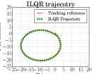
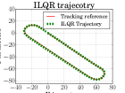
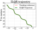
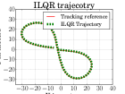
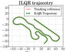
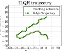
We evaluate the performance of the trajectory tracking algorithm by using four metrics, average cross track error(ACE), maximum cross track error(MCE), average velocity error(AVE) and maximum velocity(MVE). For Polaris GEM e6 we calculate these metrics on five types of reference trajectories namely circular track ‘Fig. 4(a)’, oval track ‘Fig. 5(a)’, snake track ‘Fig. 6(a)’, ’Eight’ track ‘Fig. 7(a)’, and a combination track ‘Fig. 8(a)’. We collect the reference trajectories by logging the VectorNav-300 GPS data while driving manually. We evaluate Warthog’s performance on the reference trajectory shown in ‘Fig. 9(a)’ which involves moving at the speeds of 3m/s-4m/s, mimicking the kind of trajectories Warthog might be required to follow in an off-road environment. The warthog has a maximum velocity of 4.5m/s so we are testing the controller at the limits of what the Warthog can perform.

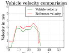
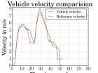
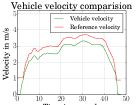
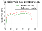
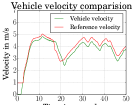
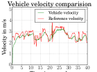
‘Table I’ summarizes the results of these experiments on both Warthog and Polaris GEM e6. Both vehicles are equipped with a VectorNav-300 GPS for localization which is accurate up to 20-30 cm, considering the GPS accuracy the ACEs and MCEs are acceptable for both Polaris GEM e6 and Warthog. The reason for high MVEs is the fact that at the start vehicle has zero velocity while the initial points in the reference trajectories have 1m/s-2m/s velocities. The high MCE for ’Eight’ track is due to the 0.8m/s reference velocity reported by GPS around 25th second from starting time as shown in ‘Fig. 7(b)’.

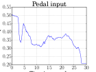
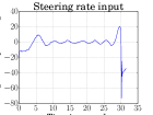
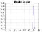
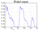
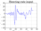
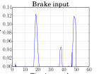
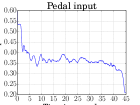
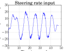
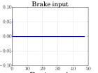
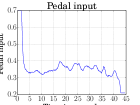
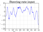
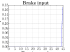
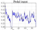
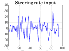
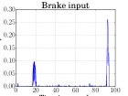
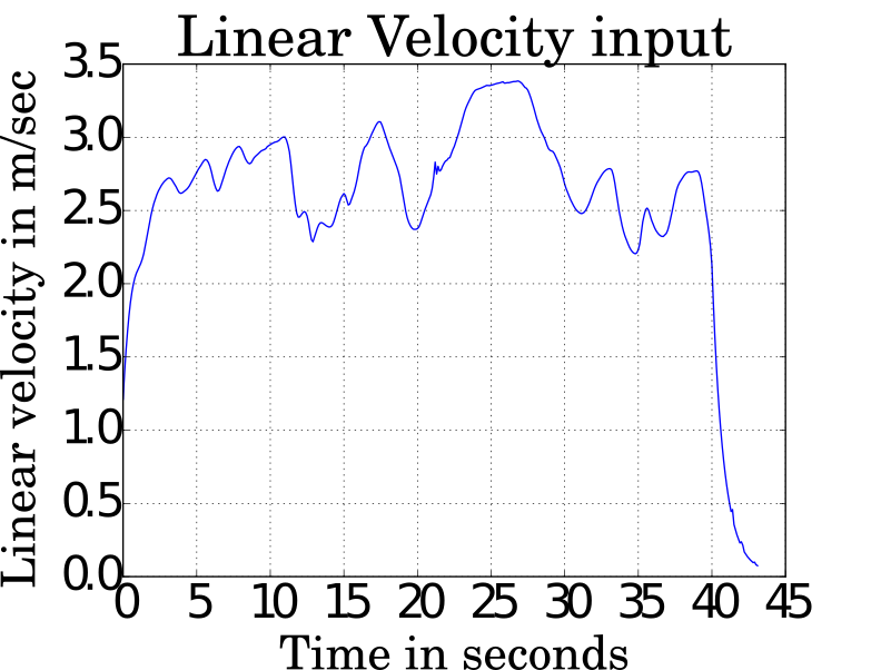
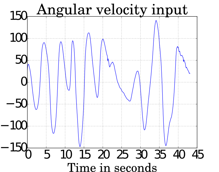
‘Fig. [4-9](b)’ compare commanded velocities and actual vehicle velocities for the reference trajectories. The control input plots ‘Fig. [4-8][c-e]’ and ‘Fig. 9[c-d]’ show that the control inputs satisfy the predefined constraints of $[0,1]$ for pedal and brake, $[-60,60]$ for steering rate(deg/s), $[0,4.5]$ for Warthog linear velocity (m/s) and $[-180,180]$ for Warthog angular velocity (deg/s).

In this work we demonstrated a model based control methodology for an off-road vehicle as well as an on-road shuttle with varying dynamics, speeds as well as environmental conditions. In future we plan to compare this approach with classical geometric and dynamic controllers for wheeled robots in trajectory following context. We also plan to implement the controller presented in this paper on an eighteen wheeler with a trailer attached. Truck and a trailer has a complex non linear dynamics and is a challenging problem what will further test the limits of the controller presented in this work.

(a)

(b)

(c)

(d)

(e)

Figure 4: Polaris GEM e6 Circular trajectory response

(a)

(b)

(c)

(d)

(e)

Figure 5: Polaris GEM e6 Oval trajectory response

(a)

(b)

(c)

(d)

(e)

Figure 6: Polaris GEM e6 Snake trajectory response

(a)

(b)

(c)

(d)

(e)

Figure 7: Polaris GEM e6 Eight trajectory response

(a)

(b)

(c)

(d)

(e)

Figure 8: Polaris GEM e6 Combination trajectory response

(a)

(b)

(c)

(d)

Figure 9: Warthog Combination trajectory response

Error Metrics
Reference	ACE	MCE	AVE	MVE
GEM Circular	0.24m	0.61m	0.44m/s	1.73m/s
GEM Oval	0.32m	0.66m	0.48m/s	1.61m/s
GEM Snake	0.40m	0.72m	0.46m/s	1.02m/s
GEM Eight	0.44m	1.32m	0.58m/s	3.88m/s
GEM Combination	0.43m	0.89m	0.43m/s	2.10m/s
Warthog Combination	0.25m	0.56m	0.28m/s	2.46m/s

TABLE I: Error result on various reference Trajectories.

References

- [1] “Polaris gem e6,” https://gem.polaris.com/en-us/e6/.
- [2] M. Deisenroth and C. Rasmussen, “Pilco: A model-based and data-efficient approach to policy search,” in Proceedings of the 28th International Conference on Machine Learning, ICML 2011. Omnipress, 2011, pp. 465–472.
- [3] J. Morimioto, G. Zeglin, and C. G. Atkeson, “Minimax differential dynamic programming: application to a biped walking robot,” in SICE 2003 Annual Conference (IEEE Cat. No.03TH8734), vol. 3, Aug 2003, pp. 2310–2315 Vol.3.
- [4] D. Meger, J. C. G. Higuera, A. Xu, P. Giguère, and G. Dudek, “Learning legged swimming gaits from experience,” in 2015 IEEE International Conference on Robotics and Automation (ICRA), May 2015, pp. 2332–2338.
- [5] H. Durrant-Whyte, N. Roy, and P. Abbeel, Learning to Control a Low-Cost Manipulator Using Data-Efficient Reinforcement Learning, 2012, pp. 57–64.
- [6] M. P. Deisenroth, G. Neumann, and J. Peters, “A survey on policy search for robotics,” Foundations and Trends in Robotics, vol. 2, pp. 1–142, 2013.
- [7] J. Kober, J. A. Bagnell, and J. Peters, “Reinforcement learning in robotics: A survey,” I. J. Robotics Res., vol. 32, pp. 1238–1274, 2012.
- [8] C. E. Garcia, D. M. Prett, and M. Morari, “Model predictive control: Theory and practice - a survey,” Autom., vol. 25, pp. 335–348, 1989.
- [9] J. Schulman, S. Levine, P. Moritz, M. I. Jordan, and P. Abbeel, “Trust region policy optimization,” CoRR, vol. abs/1502.05477, 2015. [Online]. Available: http://arxiv.org/abs/1502.05477
- [10] Y. Tassa, T. Erez, and E. Todorov, “Synthesis and stabilization of complex behaviors through online trajectory optimization,” in International Conference on Intelligent Robots and Systems, 2012.
- [11] K. Hornik, “Approximation capabilities of multilayer feedforward networks,” Neural Netw., vol. 4, no. 2, p. 251–257, Mar. 1991. [Online]. Available: https://doi.org/10.1016/0893-6080(91)90009-T
- [12] B. Hanin and M. Sellke, “Approximating Continuous Functions by ReLU Nets of Minimal Width,” arXiv e-prints, p. arXiv:1710.11278, Oct 2017.
- [13] S. Dargan, M. Kumar, M. R. Ayyagari, and G. Kumar, “A survey of deep learning and its applications: A new paradigm to machine learning,” Archives of Computational Methods in Engineering, Jun 2019. [Online]. Available: https://doi.org/10.1007/s11831-019-09344-w
- [14] K. S. Narendra and K. Parthasarathy, “Identification and control of dynamical systems using neural networks,” IEEE Transactions on Neural Networks, vol. 1, no. 1, pp. 4–27, March 1990.
- [15] S. CHEN, S. A. BILLINGS, and P. M. GRANT, “Non-linear system identification using neural networks,” International Journal of Control, vol. 51, no. 6, pp. 1191–1214, 1990. [Online]. Available: https://doi.org/10.1080/00207179008934126
- [16] S. Elanayar V.T. and Y. C. Shin, “Radial basis function neural network for approximation and estimation of nonlinear stochastic dynamic systems,” IEEE Transactions on Neural Networks, vol. 5, no. 4, pp. 594–603, July 1994.
- [17] A. Draeger, S. Engell, and H. Ranke, “Model predictive control using neural networks,” IEEE Control Systems Magazine, vol. 15, no. 5, pp. 61–66, Oct 1995.
- [18] J. Kocijan, R. Murray-Smith, C. E. Rasmussen, and A. Girard, “Gaussian process model based predictive control,” in Proceedings of the 2004 American Control Conference, vol. 3, June 2004, pp. 2214–2219 vol.3.
- [19] J. Ko, D. J. Klein, D. Fox, and D. Haehnel, “Gaussian processes and reinforcement learning for identification and control of an autonomous blimp,” in Proceedings 2007 IEEE International Conference on Robotics and Automation, April 2007, pp. 742–747.
- [20] D. Nguyen-Tuong and J. Peters, “Local gaussian process regression for real-time model-based robot control,” in 2008 IEEE/RSJ International Conference on Intelligent Robots and Systems, Sep. 2008, pp. 380–385.
- [21] G. Cao, E. M. Lai, and F. Alam, “Gaussian process model predictive control of unmanned quadrotors,” in 2016 2nd International Conference on Control, Automation and Robotics (ICCAR), 2016, pp. 200–206.
- [22] M. Deisenroth, D. Fox, and C. Rasmussen, “Gaussian processes for data-efficient learning in robotics and control,” IEEE Transactions on Pattern Analysis & Machine Intelligence, vol. 37, no. 02, pp. 408–423, feb 2015.
- [23] S. Kamthe and M. Deisenroth, “Data-efficient reinforcement learning with probabilistic model predictive control,” CoRR, vol. abs/1706.06491, 2017. [Online]. Available: http://arxiv.org/abs/1706.06491
- [24] K. Chua, R. Calandra, R. McAllister, and S. Levine, “Deep reinforcement learning in a handful of trials using probabilistic dynamics models,” CoRR, vol. abs/1805.12114, 2018. [Online]. Available: http://arxiv.org/abs/1805.12114
- [25] D. H. Jacobson and D. Q. Mayne, “Differential dynamic programming,” Modern Analytic and Computational Methods in Science and Mathematics, no. 24, 1970.
- [26] W. Li and E. Todorov, “Iteraitve linear quadratic regulator design for nonlinear biological movement systems,” in International Conference on Informatics in Control, Automation and Robotics, 2004.
- [27] E. Todorov and W. Li, “A generalized iterative lqg method for locally-optimal feedbackcontrol of constrained nonlinear stochastic systems,” in American Control Conference, 2005.
- [28] J. van dan Berg, “Extended lqr: Locally-optimal feedback control for systems with non-linear dynamics and non-quadratic cost,” in International Symposium of Robotics Research, 2013.
- [29] J. van den Berg, “Iterated lqr smoothing for locally-optimal feedback control of systems with non-linear dynamics and non-quadratic cost,” in 2014 American Control Conference, June 2014, pp. 1912–1918.
- [30] Y. Tassa, N. Mansard, and E. Todorov, “Control-limited differential dynamic programming,” in 2014 IEEE International Conference on Robotics and Automation (ICRA), May 2014, pp. 1168–1175.
- [31] J. Chen, W. Zhan, and M. Tomizuka, “Constrained iterative lqr for on-road autonomous driving motion planning,” in 2017 IEEE 20th International Conference on Intelligent Transportation Systems (ITSC), Oct 2017, pp. 1–7.