Restrain the losses of the entanglement and the non-local advantage of quantum coherence for accelerated quantum systems

Abstract

We examined the possibility of recovering the losses of entanglement and the non-local advantage by using the local symmetric operations. The improvement efficiency may be increased by applying the symmetric operations on both qubits. The recovering process of both phenomenon is exhibited clearly when only one qubit is accelerated and the symmetric operations is applied on both qubits. It is shown that, for large acceleration, the non-local coherent advantage may be re-birthed by using these symmetric operations.

Keywords : non-local coherent advantage ($\mathcal{N}_{La}$), acceleration, quantum coherence, parity-time ($\mathcal{PT}$)-symmetric operation.

1 Introduction

Quantum coherence is one of the most essential principles of quantum physics that plays a crucial role in many promising fields such as quantum biology [1, 2] and quantum thermodynamics [3, 4]. Some theoretical framework concerning the measure of coherence of quantum states are given in [5, 6, 7, 8]. Specifically, Baumgratz et al. [5] introduced some criteria that must be satisfied by any good measure of coherence.

In this contribution, we consider the $l_{1}$-norm and the relative entropy of coherence as a measure of quantum coherence, where these measures satisfy the criteria suggested by Baumgratz et al [5]. For a combined system $AB$, we quantify the non-local advantage $\mathcal{N}_{La}$ on party $B$ by local measurements on party $A$ and classical communication between its two parties [9]. However, it is well known that the Unruh effect on the accelerated systems causes degradation of entanglement [10] and consequently, the coherence between the accelerated subsystems decreases. Moreover, the decay rate of the coherence increases if the accelerated systems are subject to extra noise. Recently, researchers have been interested in investigating the behavior of accelerated systems in different types of noise. For example, Metwally [11] showed that there is a more robust use of the generic pure state than the self-transposed classes and the optimum communication between the users for small values of the acceleration is investigated in [12].

In our approach, to investigate the possibility of enhancing the non-local coherent advantage of the accelerated system, we use the non-Hermitian local symmetric operator, ($\mathcal{PT}$) [13], where it has been shown, that this operator can be used to minimize the losses of entanglement [14]. Also, Guo et al [15] used this symmetric operator to suppress decoherence and enhance the parameter estimation precision. So, in this contribution, we assume that a combined system, initially prepared in a maximum entangled state of Bell type, is accelerated: either one or both subsystems are accelerated. Due to the acceleration the decoherence phenomena appears and consequently the entanglement degraded. We estimate the loss of the non-local coherent advantage and by means of the negativity we quantify the entanglement. The possibility of protecting and minimizing the decay of these two phenomena are achieved by using the symmetric operator, where different possibilities are considered.

The paper is organized as follows. In Sec. 2, we describe briefly the acceleration process of the initial system, where it is assumed that either one or both subsystems are accelerated. The amount of the survival amount of entanglement is quantified using the negativity measure. The mathematical form of the non-local coherent advantage is introduced in Sec. 2.2, where, we investigate the decay behavior of this phenomena due to the acceleration process. The improving process of the entanglement and the non-local coherent advantage is discussed in Sec. 3, where different scenarios are introduced. In Sec. 4, we investigate numerically, the possibility of improving the entanglement of the accelerated systems. Sec. 5, is devoted to discuss the behavior of the non-local coherent advantage in the presence of the symmetric operators, where it is shown that by controlling on the operator strength, one can protect the loss of this phenomena. Finally, our results are summarized in Sec. 6.

2 The system and its evaluation

2.1 Acceleration Process

Assume that, we have a quantum system initially prepared in a maximum entangled state of Bell type as,

$$|\psi_{0}\rangle=\frac{1}{\sqrt{2}}(|0_{A}0_{B}\rangle+|1_{A}1_{B}\rangle).$$ (1)

It is assumed that, either one or both subsystems are accelerated. The acceleration process is performed with the computational basis, $|0_{R}\rangle$ and $|1_{R}\rangle$, in the Minkowski space $(t,z)$ of the qubit state is transformed into the Rindler space $(\tau,x)$ using the transformations [16, 17].

$$\tau=r~{}tanh\left(\frac{t}{z}\right),\quad x=\sqrt{t^{2}-z^{2}},$$ (2)

where $-\infty<\tau<\infty$, $-\infty<x<\infty$ and $r$ is the acceleration of the moving particle. Note that, the Minkowsik coordinates $(t,z)$ and Rindler coordinates $(\tau,x)$ are used to describe Dirac field, in the inertial and non-inertial frames, respectively. The relations (2) describe two regions in Rindler’s spaces: the first region $I$ for $t>|z|$ and the second region $II$ for $t<-|z|$ [18]. Therefore the basis $|0_{R}\rangle$ and $|1_{R}\rangle$, can be transformed as,

$$\begin{aligned} |0_{R}\rangle&=\cos(r)|0_{I}\rangle|0_{II}\rangle+\sin(r)|1_{I}\rangle|1_{II}\rangle,\\ |1_{R}\rangle&=|1_{I}\rangle|0_{II}\rangle.\end{aligned}$$ (3)

If only the first qubit is accelerated, then the final accelerated state in the first region $I$ is given by,

$$\rho(0)_{A,I_{acc}}=\left(\begin{array}[]{cccc}\frac{\cos^{2}(r)}{2}&0&0&\frac{\cos(r)}{2}\\ 0&\frac{\sin^{2}(r)}{2}&0&0\\ 0&0&0&0\\ \frac{\cos(r)}{2}&0&0&\frac{1}{2}\\ \end{array}\right).$$ (8)

Similarly, if the two subsystems are accelerated, then the final accelerated state in the first region $I$ is given by

$$\rho(0)_{A_{acc},I_{acc}}=\left(\begin{array}[]{cccc}\frac{\cos^{4}(r)}{2}&0&0&\frac{\cos^{2}(r)}{2}\\ 0&\frac{1}{8}\sin^{2}(2r)&0&0\\ 0&0&\frac{1}{8}\sin^{2}(2r)&0\\ \frac{\cos^{2}(r)}{2}&0&0&\frac{1}{2}\mu\\ \end{array}\right),$$ (13)

where $\mu=(\sin^{4}(r)+1)$.

Figure 1: In the absence of the $\mathcal{PT}$-local, the behavior of the negativity, $\mathcal{N}_{eg}$ of the accelerated system is described in Fig(a),(b), when Alice’qubit or both qubits are accelerated, respectively.

To quantify the amount of entanglement between the two subsystems, we use one of the most common quantitative measures of entanglement, namely, the negativity [19, 20]. Mathematically it is defined by,

$$\mathcal{N}_{eg}=max[0,-2\min\{\lambda_{\mu}\}],$$ (14)

where $\{{\lambda_{\mu}}\},~{}\mu=1..4$ represent the eigenvalues of $\rho_{ab}^{T_{2}}$ and $T_{2}$ refers to the partial transposition for the second subsystem. For a maximally-entangled state the negativity is maximum, i.e., $\mathcal{N}_{eg}=1$, while for the product states, $\mathcal{N}_{eg}=0$ [20, 21]. Fig.(1), shows the behavior of the survival amount of entanglement by means of negativity: at zero acceleration $(r=0)$, the negativity is maximum, $\mathcal{N}_{eg}=1$. As the acceleration increases, the negativity decreases to reach its minimum values at $r=0.8$. It is noted from Figs.(1a) and (1b) that, the decay rate of negativity relatively increases, when both qubits are accelerated.

2.2 The non-local advantage, $\mathcal{N}_{La}$

We start by recalling one of the favourite measures of coherence, namely, the one norm coherence $C_{l_{1}}^{na1}$. For any density operator $\rho_{ij}$ it is defined on the basis ${|i\rangle}_{i=1}^{d}$ as,

$$\begin{aligned} C_{l_{1}}^{na1}&=\sum_{i\neq j}|\langle i|\rho_{ij}|j\rangle|.\end{aligned}$$ (15)

Let us assume that the two users Alice and Bob share two qubit- state, $\rho_{AB}$. Let, t Alice who hold the first qubit $(A)$, performs a local measurements $\prod_{i}^{a}=\frac{1}{2}(I_{2}+(-1)^{a}\sigma_{i})$ on her qubit $A$ and informs Bob of her randomly selected observable $\sigma_{i}$ and the measurement results $a\in\{0,1\}$, where $\sigma_{i}$ being one of the Pauli operators $\sigma_{x,y,z}$ and $I_{2}$ is the 2-dimensional identity operator. By averaging over the three possible measurements of Alice and the corresponding eigenbases choosen by Bob, Mondal et al [22] derived the criterion for achieving the non-local advantage of quantum coherence ( NAQC)

$$\tilde{C}_{\alpha}^{na}=\frac{1}{2}\sum_{\begin{subarray}{c}i,j,a\\ i\neq j\end{subarray}}p_{a|\prod_{i}^{a}}C_{\alpha}^{\sigma_{j}}(\rho_{B|\prod_{i}^{a}})>C_{\alpha}^{m},$$ (16)

where $C_{\alpha}^{\sigma_{j}}(.)$($\alpha=l_{1}$ ) represents the quantum coherence with respect to the reference basis spanned by the eigenstates of $\sigma_{j}$, and the two critical values are given by $C_{l_{1}}^{m}=\sqrt{6}$. The probability for Alice’s measurement is $p_{a|\prod_{i}^{a}}=Tr[(\prod_{i}^{a}\otimes I_{2})\rho_{AB}]$, and $\rho_{B|\prod_{i}^{a}}$ is the corresponding postmeasurement state defined as,

$$\rho_{B|\prod_{i}^{a}}=\frac{Tr_{A}[(\prod_{i}^{a}\otimes I_{2})\rho_{AB}]}{p_{a|\prod_{i}^{a}}}.$$ (17)

Based on the criterion of equation 16, Hu et al[23] proposed to characterize quantitatively the degree of $\mathcal{N}_{La}$ of bipartite state as,

$$\mathcal{N}_{La}(\rho_{AB})=\max\{0,\frac{\tilde{C}_{\alpha}^{na}(\rho_{AB})-C_{\alpha}^{m}}{\tilde{C}_{\alpha,\max}^{na}-C_{\alpha}^{m}}\},$$ (18)

where $\tilde{C}_{\alpha,\max}^{na}=\max_{\rho_{AB}\in D(C^{d\times d})}\tilde{C}_{\alpha}^{na}(\rho_{AB})$ and for the two-qubit states we have $\tilde{C}_{\alpha,\max}^{na}=3$.

Figure 2: The behavior of the non-local advantage , $\mathcal{N}_{La}$ of the accelerated system (a) only qubit system is accelerated and (b)the two qubits are accelerated, respectively.

In Fig.(2), we plot the non-local advantage $\mathcal{N}_{La}$ for the accelerated system in the absence of the local $\mathcal{PT}$-symmetric operator. As seen $\mathcal{N}_{La}$, decreases as the acceleration increases. However, when only one qubit is accelerated,(see Fig.(2a)) $\mathcal{N}_{La}$ decreases gradually in Fig.(2b), it decays faster if both qubits are accelerated and vanishes at small values of acceleration, $r>0.55$ and survives for large acceleration if only one qubit is accelerated.

3 The evaluation of the system

In this section, we use the $\mathcal{PT}$-symmetric operator [13] to recover the losses of quantum entanglement and the non local advantage , as well as, the possibility of restraining their decay, $\mathcal{N}_{La}$. This symmetric operator, $\mathcal{PT}$ is defined as,

$$\mathcal{H}_{\mathcal{PT}}=\left(\begin{array}[]{cc}i\sin(\alpha)&1\\ 1&-i\sin(\alpha)\\ \end{array}\right),$$ (21)

where $\alpha$ is the real number characterizes the non-Hermitically if $\rvert\alpha\lvert<\frac{\pi}{2}$, while $\alpha=0$ corresponds to $H_{\mathcal{PT}}$ Hermitian. The time-evolving operator of $\mathcal{H}_{\mathcal{PT}}$ according to non-Hermitian quantum theory [13, 14] is written as,

$$U_{\mathcal{PT}}=\exp(-i\mathcal{H}_{\mathcal{PT}}t)=\sec(\alpha)\left(\begin{array}[]{cc}\cos(\alpha-\alpha_{1})&-i\sin(\alpha_{1})\\ -i\sin(\alpha_{1})&\cos(\alpha+\alpha_{1})\\ \end{array}\right),$$ (24)

where $\alpha_{1}=t\cos(\alpha)$. Now, we consider the following cases:

1. Only one qubit is accelerated

   Here we assume that, the users Alice and Bob share the state(3), where only one qubit is accelerated. If the symmetric operator is applied on the first qubit only, then the output state is defined as:

   $$\rho(t) = \frac{(U_{\mathcal{PT}}\otimes I_{B})\varrho_{A,I_{acc}}(U_{\mathcal{PT}}\otimes I_{B})^{\dagger}}{Tr[(U_{\mathcal{PT}}\otimes I_{B})\varrho_{A,I_{acc}}(U_{\mathcal{PT}}\otimes I_{B})^{\dagger}]}$$ (25)

   where the final density operator $\rho(t)$ on the computational basis is defined by the elements,

   $$\begin{aligned} \rho_{11}&=\frac{\delta^{2}}{2Z}\cos^{2}(r),\\ \rho_{12}&=\frac{i\nu\delta}{2Z}\cos(r),\\ \rho_{13}&=\frac{i\nu\delta}{2Z}\cos^{2}(r),\\ \rho_{14}&=\frac{\beta\delta}{2Z}\sec(\alpha)\cos(r),\\ \rho_{22}&=\frac{1}{2Z}(\nu^{2}+\sin^{2}(r)\delta^{2}),\\ \rho_{23}&=\frac{\nu^{2}}{2Z}\cos(r),\end{aligned}\qquad\begin{aligned} \rho_{24}&=-\frac{i\nu}{2Z}(\sec(\alpha)\beta-\sin^{2}(r)\delta),\\ \rho_{33}&=\frac{\nu^{2}}{2Z}\cos^{2}(r),\\ \rho_{34}&=-\frac{i\beta}{2Z}\sec^{2}(\alpha)\sin(\alpha_{1})\cos(r),\\ \rho_{44}&=\frac{1}{2Z}\sec^{2}(\alpha)(\beta^{2}+\sin^{2}(\alpha_{1})\sin^{2}(r)),\\ Z&=\sec^{2}(\alpha)-\tan^{2}(\alpha)\cos(2\alpha_{1}),\\ \rho_{21}&=\rho_{12}^{\ast},~{}~{}\rho_{31}=\rho_{13}^{\ast},~{}~{}\rho_{32}=\rho_{23},~{}~{}\rho_{41}=\rho_{14},~{}~{}\rho_{42}=\rho_{24}^{\ast},\\ \rho_{43}&=\rho_{34}^{\ast},~{}~{}\delta=\tan(\alpha)\sin(\alpha_{1})+\cos(\alpha_{1}),\\ \beta&=\cos(\alpha+\alpha_{1})~{}~{}\nu=\sec(\alpha)\sin(\alpha_{1}).\end{aligned}$$ (26)

   The second possibility is applying the symmetric-operator ( 24) on both qubits. In this case, the final output state is defined as,

   $$\rho(t) = \frac{(U_{\mathcal{PT}}\otimes U_{\mathcal{PT}})\varrho_{A,I_{acc}}(U_{\mathcal{PT}}\otimes U_{\mathcal{PT}})^{\dagger}}{Tr[(U_{\mathcal{PT}}\otimes I_{B})\varrho_{A,I_{acc}}(U_{\mathcal{PT}}\otimes I_{B})^{\dagger}]}$$ (27)

   where its elements are given by,

   $$\rho_{11} = \frac{1}{2Z}(\xi^{2}\sec^{2}(\alpha)+\xi^{2}\sin^{2}(\alpha)\cos^{2}(r)+\xi^{2}\tan^{2}(\alpha)(\sin^{2}(r)-2\cos(r))+\cos^{2}(\alpha_{2})\cos^{2}(r)),$$

   $$\rho_{12} = \frac{\xi}{Z}\tan(\alpha)\sin^{2}(\frac{r}{2})(\cos(\alpha_{2})+i(2\sec^{2}(\alpha)-1)\sin(\alpha_{2})),$$

   $$\rho_{13} = \frac{\xi}{4Z}\tan(\alpha)(e^{-i\alpha_{2}}(-2\cos(r)+\cos(2r)+1)-4i\sec^{2}(\alpha)\sin(\alpha_{2})\omega),$$

   $$\rho_{14} = \frac{1}{2Z}(-2\xi^{2}\tan^{2}(\alpha)+\cos(r)(\xi^{2}(\sin^{2}(\alpha)+\sec^{2}(\alpha))+\cos^{2}(\alpha_{2}))-i\xi(\sec(\alpha)\cos(\alpha_{2})\sin^{2}(r))),$$

   $$\rho_{21} = \frac{1}{2Z}\tan(\alpha)\xi\sin^{2}(\frac{r}{2})(2\cos(\alpha_{2})+i\xi\sec(\alpha)(\cos(2\alpha)-3)),$$

   $$\rho_{22} = \frac{1}{2Z}\sin^{2}(r)(\xi^{2}\sin^{2}(\alpha)+\cos^{2}(\alpha_{2}))+2\tan^{2}(\alpha)\xi^{2}\sin^{4}(\frac{r}{2}),$$

   $$\rho_{23} = \frac{\xi}{2Z}\sec(\alpha)(-2\tan^{2}(\alpha)\sin(\alpha_{2})\omega+i\cos(\alpha_{2})\sin^{2}(r)),$$

   $$\rho_{24} = \frac{1}{4Z}\tan(\alpha)\xi\sin^{2}(\frac{r}{2})(-4\cos(\alpha_{2})(\cos(r)+2)-4i\sin(\alpha_{2})(\cos(r)-2\tan^{2}(\alpha))),$$

   $$\rho_{31} = \frac{\xi}{4Z}\tan(\alpha)(4i\xi\sec(\alpha)\omega+e^{i\alpha_{2}}(-2\cos(r)+\cos(2r)+1)),$$

   $$\rho_{33} = \frac{\xi^{2}}{2Z}\sec^{2}(\alpha)\sin^{2}(\frac{r}{2})(\cos(2\alpha)\omega+\cos(r)+3),$$

   $$\rho_{34} = \frac{i\xi}{Z}\tan(\alpha)\sin^{2}(\frac{r}{2})((2\sec^{2}(\alpha)-1)\sin(\alpha_{2})+i\cos(\alpha_{2})),$$

   $$\rho_{43} = \frac{i\xi}{Z}\tan(\alpha)\sin^{2}(\frac{r}{2})(-2\xi\sec(\alpha)+\sin(\alpha_{2})+i\cos(\alpha_{2})),$$

   $$\rho_{44} = \frac{1}{4Z}(2\cos^{2}(\alpha_{2})+\xi^{2}(4\sec^{2}(\alpha)+(-4\tan^{2}(\alpha)\cos(r)+\cos(2r)-5)+2\sin^{2}(\alpha_{2}))),$$

   $$\rho_{32} = \rho_{23},~{}~{}\rho_{41}=\rho_{14}^{\ast},~{}~{}\rho_{42}=\rho_{24}^{\ast},~{}~{}Z=8\tan^{2}(\alpha)\xi^{2}\sin^{2}(\frac{r}{2})+1,$$

   $$\alpha_{2} = tcos^{2}(\alpha),~{}~{}\xi=\sec(\alpha)\sin(\alpha_{2}),~{}~{}\omega=(\cos(r)-1).$$ (28)

2. Both qubits are accelerated: In the second case, we consider that both subsystems are accelerated, namely the users share the state (4). If the symmetric operator ( 24) is applied on one qubit only, then the final output state is defined as $4\times 4$ matrix, where its elements are given by,

   $$\begin{aligned} \rho_{11}&=\frac{1}{8Z}(\nu^{2}\sin^{2}(2r)+4\cos^{4}(r)\delta^{2}),~{}\quad\rho_{12}=\frac{i\delta\nu}{2Z}\cos^{2}(r),\\ \rho_{13}&=-\frac{i\nu}{8Z}(\sec(\alpha)\sin^{2}(2r)\beta-4\cos^{4}(r)\delta),~{}\quad\rho_{14}=\frac{\beta\delta}{2Z}\sec(\alpha)\cos^{2}(r),\\ \rho_{22}&=\frac{1}{8Z}\sec^{2}(\alpha)(\sin^{2}(2r)\cos^{2}(\alpha-\alpha_{1})+4\sin^{2}(\alpha_{1})\mu),~{}\quad\rho_{23}=\frac{\nu^{2}}{2Z}\cos^{2}(r),\\ \rho_{24}&=-\frac{i\nu}{8Z}(4\sec(\alpha)\mu\beta-\sin^{2}(2r)\delta),~{}\quad\rho_{33}=\frac{1}{8Z}\sec^{2}(\alpha)(\sin^{2}(2r)\beta^{2}+4\sin^{2}(\alpha_{1})\cos^{4}(r)),\\ \rho_{34}&=-\frac{i\beta}{2Z}\sec^{2}(\alpha)\sin(\alpha_{1})\cos^{2}(r),~{}\quad\rho_{44}=\frac{1}{8Z}\sec^{2}(\alpha)(4\mu\beta^{2}+\sin^{2}(\alpha_{1})\sin^{2}(2r)),\\ \rho_{21}&=\rho_{12},~{}~{}\rho_{31}=\rho_{13}^{\ast},~{}~{}\rho_{32}=\rho_{23},~{}~{}\rho_{41}=\rho_{14},~{}~{}\rho_{42}=\rho_{24}^{\ast},~{}~{}\rho_{43}=\rho_{34}^{\ast},\\ Z&=\sec^{2}(\alpha)-\tan(\alpha)(\tan(\alpha)\cos(2\alpha_{1})+\sin(2\alpha_{1})\sin^{2}(r)),~{}~{}\alpha_{1}=t\cos(\alpha).\end{aligned}$$ (29)

   The final state of the initial accelerated system given by,

   $$\begin{aligned} \rho(t)&=\frac{(U_{\mathcal{PT}}\otimes U_{\mathcal{PT}})\varrho_{A_{acc},I_{acc}}(U_{\mathcal{PT}}\otimes U_{\mathcal{PT}})^{\dagger}}{Tr[(U_{\mathcal{PT}}\otimes U_{\mathcal{PT}})\varrho_{A_{acc},I_{acc}}(U_{\mathcal{PT}}\otimes U_{\mathcal{PT}})^{\dagger}]}\end{aligned},$$ (30)

   In the computational basis the elements of the density operator (19) are defined by

   $$\begin{aligned} \rho_{11}&=\frac{1}{Z}(\sec^{4}(\alpha)\gamma+\frac{\cos^{4}(r)}{2}),~{}\quad\rho_{12}=\frac{i\gamma}{Z}(\tan(\alpha)\sec^{3}(\alpha)),\\ \rho_{14}&=\frac{1}{2Z}(-2\tan^{2}(\alpha)\xi^{2}+\text{b1}\cos^{2}(r)-2i\xi(\sec(\alpha)\cos(\alpha_{2})\sin^{2}(r))),\\ \rho_{22}&=\frac{1}{8Z}\sec^{2}(\alpha)\sin^{2}(r)(-4\tan^{2}(\alpha)\cos(2\alpha_{2})+4\sec^{2}(\alpha)+2\cos(2\alpha)\cos^{2}(r)+\cos(2r)-3),\\ \rho_{23}&=\frac{\gamma}{Z}(\tan^{2}(\alpha)\sec^{2}(\alpha)),~{}\quad\rho_{24}=\frac{\lambda\xi}{Z}(\tan(\alpha)\sin^{2}(r)),\\ \rho_{33}&=\frac{1}{8Z}\sec^{2}(\alpha)\sin^{2}(r)(-4\tan^{2}(\alpha)\cos(2\alpha_{2})+4\sec^{2}(\alpha)+2\cos(2\alpha)\cos^{2}(r)+\cos(2r)-3),\\ \rho_{34}&=\frac{\lambda}{Z}(\tan(\alpha)\xi\sin^{2}(r)),\\ \rho_{41}&=\frac{1}{2Z}(\cos^{2}(r)-2\sec^{2}(\alpha)\sin(\alpha_{2})\sin^{2}(r)(\tan^{2}(\alpha)\sin(\alpha_{2})-i\cos(\alpha_{2}))),\\ \rho_{44}&=\frac{1}{2Z}(\sin^{2}(\alpha_{2})(\tan^{4}(\alpha)\mu+\cos(2\alpha)\sec^{4}(\alpha)\cos^{4}(r))+\mu\cos^{2}(\alpha_{2})),\\ \rho_{21}&=\rho_{12}^{\ast},~{}~{}\rho_{13}=\rho_{12},~{}~{}\rho_{31}=\rho_{12}^{\ast},~{}~{}\rho_{32}=\rho_{23},~{}~{}\rho_{42}=\rho_{24}^{\ast},~{}~{}\rho_{43}=\rho_{34}^{\ast}.\end{aligned}$$ (31)

   where,

   $Z=4\tan^{2}(\alpha)\sec^{2}(\alpha)\gamma+1,~{}~{}\gamma=\sin^{2}(\alpha_{2})\sin^{2}(r)~{}\quad b1=\sin^{2}(\alpha_{2})(\tan^{4}(\alpha)+\sec^{4}(\alpha))+\cos^{2}(\alpha_{2}),~{}~{}\alpha_{2}=t\cos^{2}(\alpha),\quad\lambda=(-\cos(\alpha_{2})+i\tan^{2}(\alpha)\sin(\alpha_{2}))$.

4 Recovering the entanglement

Here, we discuss the behavior of entanglement by means of the negativity, where the effect of the symmetric operator with different strengths on the negativity is investigated. It is well known that, due to the acceleration process, the decay rate of negativity increases when both qubits are accelerated.

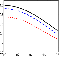
Figure 3: The behavior of the negativity $\mathcal{N}_{eg}$ of the accelerated system at different values of interaction time and for different initial settings of the $\mathcal{PT}$. It is assumed that the symmetric operator is applied only on the accelerated first qubit (a) $\alpha=\frac{\pi}{6}$, (b) $\alpha=\frac{\pi}{4}$ and (c) $\alpha=\frac{\pi}{3}$. The solid, dash and dot curves represent $\mathcal{N}_{eg}$ at $t=0.1,0.4$ and $0.9$, respectively.

In Fig.(3), it is shown the effect of the $\mathcal{PT}$ symmetric operation on the behavior of the survival amount of the entanglement by means of the negativity, $\mathcal{N}_{ng}$. The negativity decreases as $r$ increases at different values of interaction time. As, it is displayed in Fig.(3b) and (3c), the decay rate decreases as $\alpha$ decreases, where the maximum values of the negativity are improved as one increases the interaction time. Moreover, the entanglement doesn’t vanish even for large acceleration $r$.

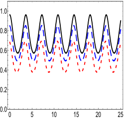
Figure 4: The behavior of the negativity $\mathcal{N}_{eg}$ in the presence of the local $\mathcal{PT}$-symmetric operator on the accelerated qubit $A$. The solid, dash and the dot lines represent $\mathcal{N}_{eg}$ at $r=0.2,0.4$ and $0.6$, respectively, where the local symmetric operator is described by (a) $\alpha=\frac{\pi}{6}$, (b) $\alpha=\frac{\pi}{4}$ and (c) $\alpha=\frac{\pi}{3}$.

The behavior of the survival amount of entanglement, $\mathcal{N}_{eg}$ is shown in Fig.(4), where it displays the instantaneous effect of the symmetric operator $\mathcal{PT}$ on the negativity. For small value of the operator strength, which is characterised by the angle $\alpha$, the negativity decays gradually to reach its minimum values. However, the decay rate increases as the acceleration increases. As one increases the operator strength, the behavior of $\mathcal{N}_{eg}$ changes dramatically, as it is displayed in Fig.(4b), where the entanglement fluctuates between its maximum and minimum values and the amplitudes of these oscillations increase and consequently,the minimum values of the negativity decrease. So, the minimum values of the negativity decreases and its the maximum values don’t exceed the initial ones. Moreover the minimum values depend on the initial values of accelerations and the operator’s strength.

Figure 5: (a) The same as Fig.(3a), where the negativity is a function of the acceleration, i.e., $\mathcal{N}_{eg}(r)$ (b) The same as Fig(4a) where the negativity is a function of the interaction time, i.e., $\mathcal{N}_{eg}(t)$. It is assumed that, the local $\mathcal{PT}$-symmetric operation on both qubits, $\alpha=\pi/6$ and only the first qubit is accelerated.

Fig(5), shows the possibility of improving the minimum values of the entanglement, when the symmetric operator is applied on both qubits. The behavior of the negativity as a function of the acceleration, $\mathcal{N}_{eg}(r)$ is displayed in Fig.(5a), where the decay rate decreases and the minimum values are much better than those displayed in Fig(3a), with the symmetric operator is applied on only one qubit. On the other hand, Fig.(5b), shows the behavior of the negativity as a function of the interaction time, $\mathcal{N}_{eg}(t)$. The depicted behavior is similar to that displayed in Fig.(4a), for the same set of parameters. However, by applying the $\mathcal{PT}$ on both qubits, the number of fluctuations decreases, where their amplitudes decrease, and consequently the minimum values are improved. Moreover, at small values of the interaction time, the maximum values are much better than those displayed at larger $t$.

Figure 6: The behavior of the negativity $\mathcal{N}_{eg}$ of the accelerated system, where it assumed that both qubits are accelerated. In Fig.(a),(b) it is assumed that the symmetric-operator is applied on only one qbit and (c), (d) it is applied on both qubits. The used parameters are the same as that used in Figs.(3a), (4a), respectively.

In reality, the two qubits may be accelerated. In this case, the behavior of the negativity depicted in Fig.(6) is similar to those predicted for cases of accelerating only one qubit in Fig.(3-4). However, due to the acceleration process of both qubits, the decay rate is much larger than that displayed in Fig.(3a) at large $r$. This phenomena is clearly displayed by comparing Fig.(3a) and Fig.(5a), where the maximum values are much larger, when only one qubit is accelerated. The possibility of improving and restraining the losses of the negativity can be achieved by applying the symmetric-operator on both qubits. As it is displayed in Fig.(5b),the negativity decays gradually and the maximum values are much better than that displayed in Fig.(6a). As it is displayed from Fig.(6b) and (6d), at small acceleration, the oscillations’ amplitude decreases when the symmetric-operator is applied on both qubits and consequently, the minimum values of the negativity are improved.

From the previous results of the negativity, it is clear that the effect of the symmetric-operator on the accelerated systems is much better when it is applied on both qubits during the interaction. However, the instant effect of the symmetric operator improve the minimum values of entanglement even at large acceleration. On the other hand, the possibility of improving the entanglement and minimizing its losses is achieved, if only one qubit is accelerated and the symmetric-operator is applied on both qubits.

In this context, it is important to mention that, our results consistences with that obtained by Chen et.al[14], where the entanglement of a two qubits system can be restored when one of them undergoes the $\mathcal{PT}$ symmetric operation and the entanglement can exceed its initial values. However, although our approach is different from that suggested by Chen et.al[14], where we applied the $\mathcal{PT}$ on accelerated systems, our conclusion is similar, where we showed that local symmetric operation improves the entanglement of the shared state between the two parties and minimize its losses.

5 Recovering the losses of $\mathcal{N}_{La}$

In this section, we investigate numerically the possibility of recovering the losses of the non-local coherent quantum advantage, where different cases will be considered: one or both qubits are accelerated, and the symmetric operator is applied either on a single or both qubits, with different initial settings of the symmetric operators.

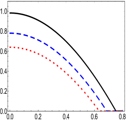
Figure 7: The behavior of the non-local coherent advantage $\mathcal{N}_{La}$ , when only one qubit is accelerated at different interaction time, where the solid, dash and dot curves are evaluated at $t=0.1,0.4$ and $0.9$, respectively, and the $\mathcal{PT}$ symmetric is described (a) $\alpha=\frac{\pi}{6}$, (b) $\alpha=\frac{\pi}{4}$ and (c) $\alpha=\frac{\pi}{3}$.

5.1 Only one qubit is accelerated

Fig.(7), shows the behavior of $\mathcal{N}_{La}$ at different interaction time, where it is assumed that the $\mathcal{PT}-operator$ is described by different angles. The general behavior is similar to that shown in Fig.(2), where the non-local coherent advantage decreases as the acceleration increases. However, at small values of the interaction time $t=0.1$, $\mathcal{N}_{La}$ decreases gradually as the acceleration increases. The maximum values of the non-local coherent advantage decreases as one increases the interaction time. Moreover, as it is displayed in Fig.(2a) $\mathcal{N}_{La}$ vanishes at small values of accelerations. Fig.(7b), show that when we increase the angle $\alpha$, which describes the strength of $\mathcal{PT}$, where we set $\alpha=\pi/4$, $\mathcal{N}_{La}$ decreases and the maximum values are much smaller than those displayed in Fig.(7a), where $\alpha=\frac{\pi}{6}$. Also, the non-local advantage survives at large values of acceleration, even at large interaction time. These phenomena is clearly exhibited in Fig.(7c), where we set $\alpha=\frac{\pi}{3}$. In this case, the maximum values of $\mathcal{N}_{La}$ are much smaller than those displayed at small values of the operator strength $\alpha$.

Figure 8: The behavior of the non-local coherent advantage, $\mathcal{N}_{La}$ in the presence of the local $\mathcal{PT}$-symmetric operator on the accelerated qubit $A$. The solid, dash and the dot lines represents the $\mathcal{N}_{La}$ at $r=0.2$, $r=0.4$ and $0.6$, respectively, where the local symmetric operator is described by (a) $\alpha=\frac{\pi}{6}$, (b) $\alpha=\frac{\pi}{4}$ and (c) $\alpha=\frac{\pi}{3}$.

The effect of the local symmetric operator $\mathcal{PT}$ on the behavior of the non-local coherent advantage, $\mathcal{N}_{La}(t)$ is shown in Fig.(8) with different initial acceleration, where it is assumed that the $\mathcal{PT}$ is applied only on one qubit. In Fig.(8a) we consider that, the symmetric operator is described by a small angle $\alpha=\pi/6$. The general behavior shows that, the non-local coherent advantage oscillates periodically between its maximum and minimum values. The minimum values depend on the initial acceleration, where as one decreases the acceleration, the minimum values are much larger than those displayed at small acceleration.

The effect of larger values of the initial angle settings of the symmetric operator is displayed in Fig.(8b), where we set $\alpha=\pi/4$. The periodic oscillations of the non-local coherent advantage are displaced with larger values of interaction time, where for large acceleration, it vanishes faster. Moreover, as the interaction time increases further, it rebirths to reach its maximum value, which doesn’t exceed its initial value.

From Fig.(8), we observe that at small values of the operator’s strength ($\alpha=\pi/6$), the behavior of the non-local coherent advantage changes dramatically, where it oscillates fast and the amplitudes of the oscillations are smaller. This means that, the minimum values of the $\mathcal{N}_{La}$ are much larger than those displayed in Figs.(8b),(8c). Moreover, the vanishing phenomena of $\mathcal{N}_{La}$ disappears and the long-lived phenomena of the non-local coherent advantage is predicted.

Figure 9: The same as Fig.(7), but it is assumed that the non local symmetric operator $\mathcal{PT}$ is applied on both qubits and only the first qubit is accelerated.

In Fig.(9), it is assumed that the symmetric operator $\mathcal{PT}$ is applied on both qubits, where only one qubit is accelerated. The general behavior shows that, $\mathcal{N}_{La}$ decays as the acceleration increases. However, at small interaction time, the decay strength induced from the acceleration is stronger than the improvement strength of the symmetric operator. The efficiency of symmetric-operator increases as one increases the interaction time, where as one increases the angle settings of the operator, the non-local coherent advantage decreases. Moreover, at $r=0$, the non-local advantage is maximum for all interaction times.

From Figs.(7) and (9), one may conclude that, the powerful of the local symmetric operator, $\mathcal{PT}$ is clearly exhibited, where one can keep the non-local coherent advantage survival and consequently the efficiency of the accelerated state increases for any value of the acceleration. By applying the local symmetric operator on both qubits, the vanishing phenomena of $\mathcal{N}_{La}$ disappears. Moreover, at zero acceleration, the effect of the symmetric operator is large, where the non-local coherent advantage is maximum and independent of the interaction time.

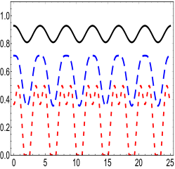
Figure 10: The same as Fig.(8), but it is assumed that, the non local symmetric operator $\mathcal{PT}$ is applied on both qubits and only the first qubit is accelerated.

Fig.(10) exhibits the improvements of the non-local advantage $\mathcal{N}_{La}$, when the symmetric operator $\mathcal{PT}$ is applied on both qubits. It is clear that, the behavior is similar to that displayed in Fig.(8a), but the number of oscillations is smaller and the amplitudes of these oscillations at small value of the interaction time, are smaller than those displayed in Fig.(8). This behavior shows that, the non-local coherent advantage is improved. The disadvantage that predicted in this figure is the vanishing phenomena of $\mathcal{N}_{La}$ at large acceleration. Moreover, as it is displayed in Figs.(10b) and (10c), the vanishing time of the non-local coherent advantage increases as the strength of the symmetric operator, $\mathcal{PT}$ increases, while, the maximum values of $\mathcal{N}_{La}$ at large acceleration ($r=0.6$, $\alpha=\pi/3$) exceeds their initial values

From, Fig.(8) and Fig.(10) one may conclude that, the non-local advantage of the accelerated system may be improved if the local symmetric operator is applied on both qubits for small acceleration. These improvements are depicted for different aspects: increasing the rate of the non-local advantage during the interaction time, with decreased vanishing time., and improvement of the maximum values to exceeds their initial values. However, the losses of the non-local advantage are not only recovered but may be increased if the local symmetric operator is applied on both qubits.

5.2 Both qubits are accelerated

In this section, we investigate the effect of the symmetric-operator on the accelerated system, where it is assumed that both qubits are accelerated. Now, we discuss the possibility of recovering the losses of the non-local advantage due to the decoherence. Similarly to the previous section, we consider two cases, one of them is assuming that the symmetric operator applies only on one qubit, while for the second case, the symmetric operator is applied on both qubits.

Figure 11: The behavior of the non-local advantage, $\mathcal{N}_{La}$, when both qubit are accelerated and the local symmetric operator is applied on only one qubits. The solid, dash and dot are evaluated $t=0.1,0.4$ and 0.9., where the strength of the operator is (a) $\alpha=\frac{\pi}{6}$, (b) $\alpha=\frac{\pi}{4}$ and (c) $\alpha=\frac{\pi}{3}$.

Fig.(11), shows the possibility of improving the non-local coherent advantage $\mathcal{N}_{La}(r)$, when both qubits are accelerated at different interaction time. The behavior is similar to that displayed in Fig.(7), where only one qubit is accelerated. However, the decay is much larger than that displayed in Fig.(7). The effect of the symmetric operator $\mathcal{PT}$, is displayed at different values of the operator’s strength. It is clear that, at small values of $\alpha$, the non-local coherent advantage, decays gradually and vanishes at large values of interaction time. However, as one increases the operator’ strength ($\alpha$), the maximum values decrease and the decay rate increases. Moreover, the non-local advantage vanishes at small values of the acceleration. As it is displayed, in Fig.(11c), $\mathcal{N}_{La}(r)$ decays fast, with maximum values are much smaller than those displayed at small values of $\alpha$.

Figure 12: The behavior of the non-local advantage, $\mathcal{N}_{La}(t)$ when the symmetric operator is applied on both qubit. The sold, dash and dot curves are evaluated at $r=0.2,0.4$ and $0.6$, respectively. The strength of the symmetric -operator is (a) $\alpha=\frac{\pi}{6}$, (b) $\alpha=\frac{\pi}{4}$ and (c) $\alpha=\frac{\pi}{3}$.

The behavior of $\mathcal{N}_{La}(t)$ is displayed in Fig.(12), where different values of the initial acceleration are considered. The fluctuations behavior of the non-local coherent advantage is displayed, where the number of oscillations decreases as the symmetric operator’ strength $\alpha$ increases. The periodic behavior shows that the amplitude of the oscillations decreases as $\alpha$ decreases and consequently, the minimum values are much large at small values of the operator’ strength. Moreover, as it is shown in Figs.(12), the non-local advantage vanishes completely with large acceleration. Further, the vanishing time of $\mathcal{N}_{La}(t)$ increases as the $\mathcal{PT}$-symmetric operator strength increases.

Figure 13: The same as Fig.(8) but the symmetric operator is applied on both qubits.

Fig.(13), we shows the possibility of recovering the losses of the non-local coherent advantage, when the $\mathcal{PT}$-symmetric operator is applied on both qubits, where different values of the initial strength are considered. The results that displayed in this figure show that, $\mathcal{N}_{La}$ is much better than that depicted in Fig.(11), where the maximum values of $\mathcal{N}_{La}$ are much better. However, as one increases the $\mathcal{PT}$-symmetric strength, the decay rate of $\mathcal{N}_{La}$ is larger than that displayed at small values of $\alpha$. Moreover, the vanishing phenomena of $\mathcal{N}_{La}$ is depicted at small values of initial accelerations.

Figs.(11) and (13), show that the possibility of imroving/recovering the non-local coherent advantage increases as the $\mathcal{PT}$-symmetric operator is applied on both qubits, where the maximum values are much larger. The only disadvantage that predicted when applying the $\mathcal{PT}$ operator on both qubits, is that the non-local coherent quantum advantage vanishes at small acceleration.

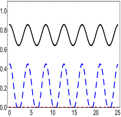
Figure 14: The same as Fig.(9) but the symmetric operator is applied on both qubits.

Fig.(14) shows the behavior of $\mathcal{N}_{La}(t)$, when the symmetric operator is applied on both qubits at different accelerations. In general, the behavior is similar to that predicted in Fig.(12), namely $\mathcal{N}_{La}(t)$ oscillates between its maximum and minimum values. However, as it is displayed in Fig.(14), the amplitude of oscillations are smaller than those shown in Fig.(12), which means that the non-local coherent advantage is improved. The most important remark is that at large accelerations, $\mathcal{N}_{La}(t)$, vanishes completely at small values of the strength $\alpha$. However, as the strength increases, the non-local coherent advantage re-births again and its maximum values increase as the strength of the symmetric operator $\alpha$ increases.

6 Conclusion

In this contribution, we investigate the possibility of recovering the loses of the entanglement and the non-local advantage for accelerated system initially prepared in the Bell state. As it is well known, due to the acceleration, the entangled properties of the accelerated system loses its coherence and consequently, their efficiency to perform some quantum information tasks decrease. One of the most important phenomena of the entanglement system, is the non-local coherent advantage of the accelerated system. We have used the local symmetric operator to improve/ recover the coherence of the non-local coherent advantage. In this context, two different cases are considered; one (both) qubits are accelerated and the symmetric operator is applied on one or both subsystems.

Due to the acceleration process, the entanglement, as quantified by means of its negativity, decreases. Possibility of improving the entanglement is suggested by using the symmetric operator. It is shown that, it can be increase instantaneously at small values of the symmetric-operator strength, where the amplitudes of the negativity oscillations decrease, and consequently its minimum values increase. The effect of the symmetric-operator on the accelerated systems is much better when it is applied on both qubits during the interaction. Moreover, this effect increases, when the symmetric operator is applied on both qubits. On the other hand, the possibility of improving and recovering the losses of entanglement increase, if only one qubit is accelerated and the symmetric-operator is applied on both qubits.

The behavior of the non-local coherent advantage decays as the acceleration increases and the decay rate is large when both qubit are accelerated. We examined the behavior of this physical phenomena at different interaction time, where different initial strength of the symmetric operator are considered. It is shown that, as the symmetric operator is applied on only one qubit, the maximum values of $\mathcal{N}_{La}(r)$ increase and vanish at large acceleration. The periodic behavior of the non-local coherent advantage is predicated, where the periodic time increases at small values of the operator strength. In addition, also $\mathcal{N}_{La}(t)$, vanishes periodically, where the disappearing interval time increases as the initial acceleration increases. However, the small values of the strength of the symmetric operator recover the losses of the $\mathcal{N}_{La}(t)$ and prevent its disappearance. Although the non-local coherent advantage fluctuates fast, the amplitudes of the oscillations are small, and in turn its minimum values are improved. Moreover, the improvement of the non-local coherent advantage is clearly displayed when only one qubit is accelerated and the local symmetric operator is applied on both qubits, where at small values of the symmetric strength $\mathcal{N}_{La}(r)$ increase and never vanishes.

The effect of the symmetric operator on the non-local coherent advantage when both qubits are accelerated is discussed. Due to the accelerating process the decay rate of $\mathcal{N}_{La}(r)$ is large. However, if the symmetric operator is applied on only one qubit, the $\mathcal{N}_{La}(r)$ increases as one decreases the strength of the symmetric operator. Similarly, the periodic behavior of $\mathcal{N}_{La}(t)$ is predicated with small amplitudes of fluctuations. These means that, the minimum values are improved. The time periodicity time increases as the strength of $\mathcal{PT}$ increases, which means that the non-local coherent advantage survives for a longer time.

Moreover, the effect of the symmetric operator on both qubits improve and recover the losses of $\mathcal{N}_{La}(r)$, where, it reaches its maximum value even at large acceleration. Therefore, if the initial acceleration is large, the decay of $\mathcal{N}_{La}(r)$ can be less by decreasing the symmetric operator strength. The amplitudes of oscillations reduce and consequently the minimum values of $\mathcal{N}_{La}(t)$ are improved. One of the important results, we obtained is: by applying the symmetric operator on both qubits, the phenomena of re-birthing the non-local coherent advantage appears. Further, the maximum values of the re-birthed non-local coherent advantage is much better than that obtained for small acceleration.

In conclusion, we examined the possibility of improving and recovering the losses of entanglement and the non-local coherent advantage by using the local symmetric-operator. The improvement efficiency may be increased by applying the symmetric operator on both qubits. The recovering process of both phenomenon is exhibited clearly when only one qubit is accelerated and the symmetric operator is applied on both qubits. It is shown that for large acceleration, the non-local coherent advantage may be re-birthed by using this symmetric operator

‏

References

- [1] Engel, G. S., Calhoun, T. R., et al. (2007). Evidence for wavelike energy transfer through quantum coherence in photosynthetic systems. Nature, 446(7137), 782.
- [2] Romero, E., Augulis, R., et al. (2014). Quantum coherence in photosynthesis for efficient solar-energy conversion. Nature physics, 10(9), 676.
- [3] Lostaglio, M., Jennings, D. and Rudolph, T. (2015). Description of quantum coherence in thermodynamic processes requires constraints beyond free energy. Nature communications, 6, 6383.
- [4] Lostaglio, M., Korzekwa, K., Jennings, D. and Rudolph, T. (2015). Quantum coherence, time-translation symmetry, and thermodynamics. Physical review X, 5(2), 021001.
- [5] Baumgratz, T., Cramer, M. and Plenio, M. B. (2014). Quantifying coherence. Physical review letters, 113(14), 140401.
- [6] Pires, D. P., Céleri, L. C. and Soares-Pinto, D. O. (2015). Geometric minimum bound for a quantum coherence measure. Physical Review A, 91(4), 042330.
- [7] Streltsov, A., Singh, U., Dhar, H. S., Bera, M. N. and Adesso, G. (2015). Measuring quantum coherence with entanglement. Physical review letters, 115(2), 020403.
- [8] Rana, S., Parashar, P. and Lewenstein, M. (2016). Trace-distance measure of coherence. Physical Review A, 93(1), 012110.
- [9] Hu, M. L. and Fan, H. (2018). Nonlocal advantage of quantum coherence in high-dimensional states. Physical Review A, 98(2), 022312.
- [10] Birrell, N. D., Birrell, N. D., Davies, P. C. W. and Davies, P. (1984). Quantum fields in curved space (No. 7). Cambridge university press.
- [11] Metwally, N. (2013). Usefulness classes of traveling entangled channels in noninertial frames. International Journal of Modern Physics B, 27(28), 1350155.
- [12] Metwally, N. and Sagheer, A. (2014). Quantum coding in non-inertial frames. Quantum information processing, 13(3), 771-780.
- [13] Bender, C. M. and Boettcher, S. (1998). Real spectra in non-Hermitian Hamiltonians having P T symmetry. Physical Review Letters, 80(24), 5243.
- [14] Chen, S. L., Chen, G. Y. and Chen, Y. N. (2014). Increase of entanglement by local -symmetric operations. Physical Review A, 90(5), 054301.
- [15] Guo, Y. N., Fang, M. F., Wang, G. Y., Hang, J. and Zeng, K. (2017). Enhancing parameter estimation precision by non-Hermitian operator process. Quantum Information Processing, 16(12), 301.
- [16] Martín-Martínez, E. and Leon, J. (2010). Quantum correlations through event horizons: Fermionic versus bosonic entanglement. Physical Review A, 81(3), 032320.
- [17] Alsing, P. M., Fuentes-Schuller, I., Mann, R. B. and Tessier, T. E. (2006). Entanglement of Dirac fields in noninertial frames. Physical Review A, 74(3), 032326.
- [18] Alsing, Paul M. and Milburn, G. J., Teleportation with a Uniformly Accelerated Partner, Phys. Rev. A.91 18, 180404 (2003).
- [19] Vidal, G. and Werner, R. F. (2002). Computable measure of entanglement. Physical Review A, 65(3), 032314.
- [20] R. Horodecki, M. Horodecki and P. Horodecki, Phys. Lett. A 222 (1996) 1; K. Zyczkowski, P. Horodecki, A. Sanpera and M. Lewenstein, Phys. Rev. A 58 (1998) 883.
- [21] Mohammed A.R. and El-Shahat T.M. (2017) . Study the Entanglement Dynamics of an Anisotropic Two-Qubit Heisenberg XYZ System in a Magnetic Field. Journal of Quantum” Information Science, 7, 160.
- [22] Mondal, D., Pramanik, T. and Pati, A. K. (2017). Nonlocal advantage of quantum coherence. Physical Review A, 95(1), 010301.
- [23] Hu, M. L., Wang, X. M. and Fan, H. (2018). Hierarchy of the nonlocal advantage of quantum coherence and Bell nonlocality. Physical Review A, 98(3), 032317.