Few-Shot Keyword Spotting With Prototypical Networks

Abstract

Recognizing a particular command or a keyword, keyword spotting has been widely used in many voice interfaces such as Amazon’s Alexa and Google Home. In order to recognize a set of keywords, most of the recent deep learning based approaches use a neural network trained with a large number of samples to identify certain pre-defined keywords. This restricts the system from recognizing new, user-defined keywords. Therefore, we first formulate this problem as a few-shot keyword spotting and approach it using metric learning. To enable this research, we also synthesize and publish a Few-shot Google Speech Commands dataset. We then propose a solution to the few-shot keyword spotting problem using temporal and dilated convolutions on prototypical networks. Our comparative experimental results demonstrate keyword spotting of new keywords using just a small number of samples.

1 Introduction

Most smart devices these days have an inbuilt voice recognition system which is mainly used for taking voice input from a user. This requires the voice recognition system to detect specific words (keywords/commands), also known as the Keyword Spotting (KWS) problem. Most approaches use either Large Vocabulary Continuous Speech Recognition (LVCSR) based models [1, 2] or lightweight deep neural network based models [3]. The former, LVCSR demands a lot of resource and computation power and hence are deployed in the cloud, raising privacy concerns and latency issues. The latter models are trained with a set of pre-defined keywords to recognize using thousands of training examples. However, with smart devices becoming more personalized, there is a growing need for such systems 1) to recognize custom or new keywords on-device and 2) to quickly adapt from a small number of user samples as the existing approaches require large number of training samples. Therefore, we attempt to solve this problem of recognizing new keywords given a few samples, hereon referred to as Few-Shot Keyword Spotting (FS-KWS).

Current approaches to KWS involves extracting audio features from the input keyword and then passing it as input to a Deep Neural Network (DNN) for classification [4, 3, 5, 6, 7]. Especially, the use of convolutional neural networks (CNNs) [8] in adjunction with Mel-frequency Cepstral Coefficients (MFCC) as speech features have shown to produce remarkable results [3, 4, 7, 9, 10].

Due to the data hungry nature of DNNs, recently the field of Few-Shot Learning has gained a lot of attention. Specifically, Few-Shot Classification (FSC) [11] aims to learn a classifier that can recognize new classes (not seen during training) when given limited, labeled examples for each new class. Broadly there are two approaches to FSC. First, Metric Learning based approaches [12, 13, 14] try to learn a good embedding function which can align examples of same class close to each other and far from examples of different class in an embedding space based on a metric (distance function). Second, Optimization based approaches [15, 16] attempts to learn good initialization parameters for a classifier such that it can be finetuned using few gradient descent steps on examples from new classes to classify them correctly. Both approaches involve training the classifier with a new set of classes in each training episode such that it will be able to classify another new set of classes at test time.

Previously, [17] have attempted to solve FS-KWS using model-agnostic meta learning (MAML) [16], an optimization based approach to FSC. However, since KWS is deployed on small devices with limited computation capability, an optimization based approach that requires fine-tuning may not always be feasible. Hence, we approach FS-KWS using metric learning based approach, specifically using Prototypical Networks [14] which can perform inference in an end-to-end manner. The following summarizes our main contributions:

• We propose a keyword spotting system that can classify new keywords from limited samples by a few-shot formulation of keyword spotting with metric learning.

• We propose a temporally dilated CNN architecture as a better embedding function for FS-KWS.

• We release a FS-KWS dataset synthesized from Google's Speech command dataset [18]. To make it more challenging, we also incorporate background noise and detection of silence and unknown (negative) keywords.

2 Few-Shot Keyword Spotting (FS-KWS) Problem

Consider a set $S$ of user-defined keywords such that $S=\{(s_{i},y_{i})\}^{N\times K}_{i}$ where $s_{i}$ is a keyword sample (voice input) and $y_{i}$ is its label. The set $S$ contains $N$ keywords, each keyword having $K$ samples where $K$ is a small number (for ex., 1,2,5). Then given a user query $q$, the objective of FS-KWS system is to classify $q$ into one of $N$ keyword classes. The user-defined keywords in $S$ could be new i.e, never seen before during the training of FS-KWS system. Yet, the system should be able to detect $q$, given $S$.

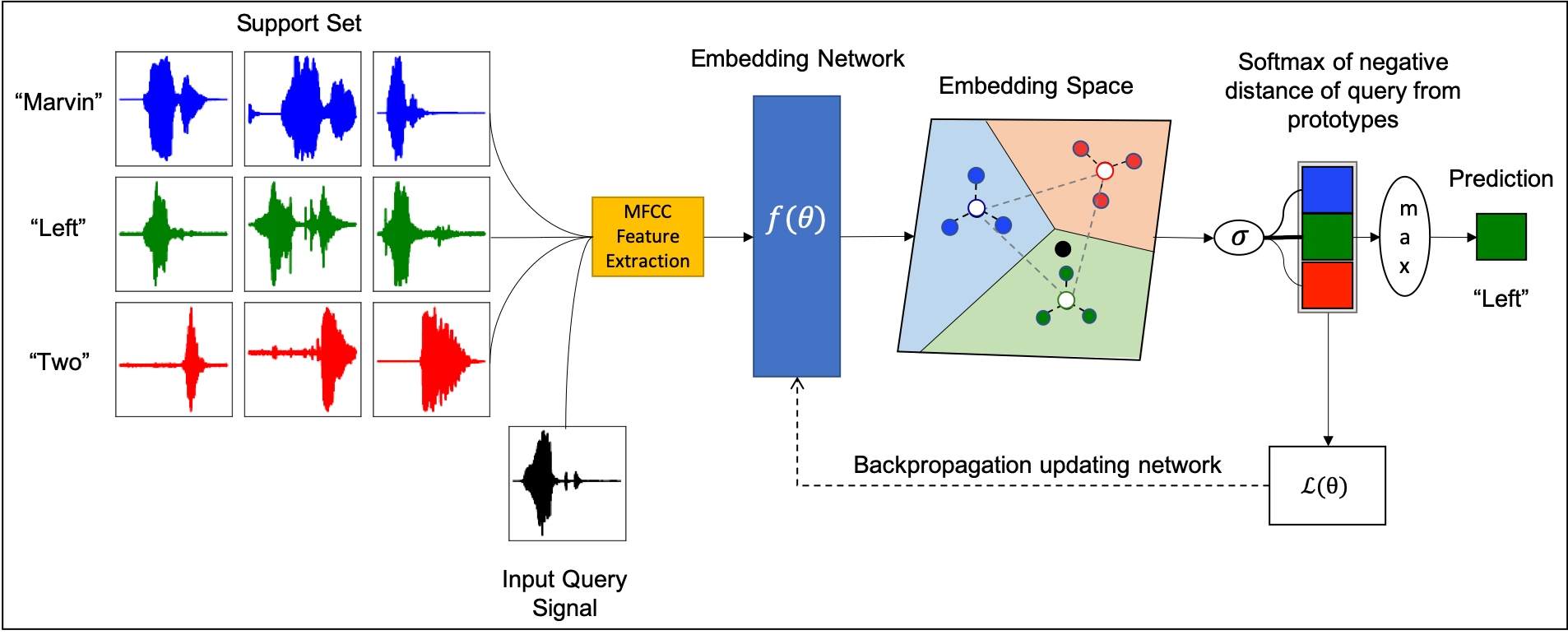
Figure 1: Few-Shot Keyword Spotting Pipeline

3 FS-KWS Framework

We base our framework (Figure 1) on Prototypical Networks [14] for building the FS-KWS system. The FS-KWS model is trained on a labeled dataset $D_{train}$ and tested on $D_{test}$. The set of keywords present in $D_{train}$ and $D_{test}$ are disjoint. The test set has only a few labeled samples per keyword. We follow an episodic training paradigm in which each episode the model is trained to solve an $N$-way $K$-Shot FS-KWS task. Each episode $e$ is created by first sampling $N$ categories from the training set and then sampling two sets of examples from these categories: (1) the support set $S_{e}=\{(s_{i},y_{i})\}_{i=1}^{N\times K}$ containing $K$ examples for each of the $N$ categories and (2) the query set $Q_{e}=\{(q_{j},y_{j})\}_{j=1}^{N\times Q}$ containing $Q$ different examples from the same $N$ categories. The episodic training for FS-KWS minimizes, for each episode, the loss of the prediction on samples in the query set, given the support set. The model is a parameterized function and the loss is the negative log likelihood of the true class of each query sample:

$$L(\theta)=-\sum_{t=1}^{|Q_{e}|}\log P_{\theta}(y_{t}\mid q_{t},S_{e}),$$ (1)

where $(q_{t},y_{t})\in Q_{e}$ and $S_{e}$ are, respectively, the sampled query and support set at episode $e$ and $\theta$ are the parameters of the model.

Prototypical networks make use of the support set to compute a centroid (prototype) for each category (in the sampled episode) and query samples are classified based on the distance to each prototype. The model is a CNN $f:\Re^{n_{v}}\to\Re^{n_{p}}$, parameterized by $\theta_{f}$, that learns a $n_{p}$-dimensional space where $n_{v}$-dimensional input samples of the same category are close and those of different categories are far apart. For every episode $e$, each embedding prototype $p_{c}$ (of category $c$) is computed by averaging the embeddings of all support samples of class $c$:

$$p_{c}=\frac{1}{|S_{e}^{c}|}\sum_{(s_{i},y_{i})\in S_{e}^{c}}f(s_{i}),$$

where $S_{e}^{c}\subset S_{e}$ is the subset of support examples belonging to class c. Given a distance function $d$, the distance of the query $q_{t}$ to each of the class prototypes $p_{c}$ is calculated. By taking a softmax [19] of the measured (negative) distances, the model produces a distribution over the $N$ categories in each episode:

$$P(y=c\mid q_{t},S_{e},\theta)=\frac{exp(-d(f(q_{t}),p_{c}))}{\sum_{n}exp(-d(f(q_{t}),p_{n}))},$$

where metric $d$ is a Euclidean distance and the parameters $\theta$ of the model are updated with stochastic gradient descent by minimizing Equation (1). Once the training finishes, the parameters $\theta$ of the network are frozen. Then, given any new FS-KWS task, the category corresponding to the maximum $P$ is the predicted category for the input query $q_{t}$.

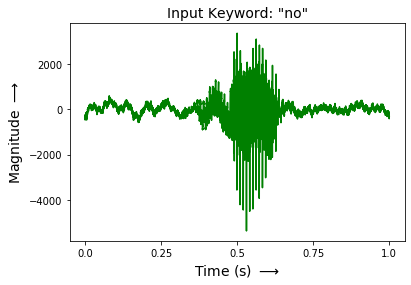
(a) Input Speech

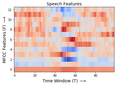
(b) MFCC Features

Figure 2: Example transformation of input speech to MFCC features

3.1 Audio Feature Extraction

In each episode, we first obtain Mel-frequency Cepstral Coefficients (MFCC) features for all the examples in the support set and the query set which then act as input to the embedding network as shown in Figure 1. Following [5], we extract 40 MFCC features from a speech frame of length 40 ms and stride 20 ms (see Figure 2).

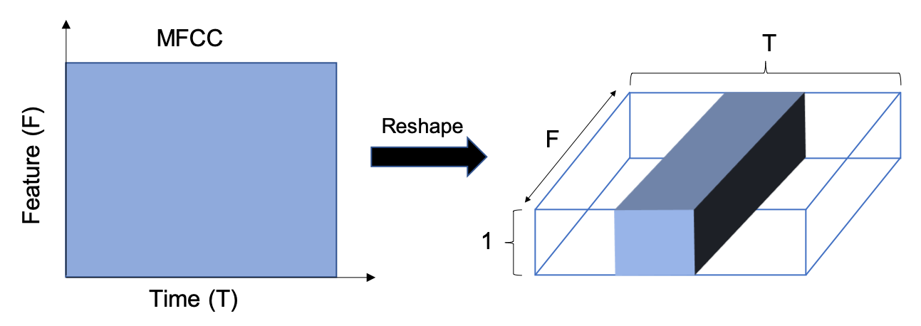
Figure 3: Reshaping MFCC features for time convolution.

3.2 Embedding Network

Choi et al. [9] demonstrated improved performance on KWS with temporal convolutions by reshaping the input MFCC features (Figure 3). Also, Cocke et al. [10] have shown that dilated convolutions are helpful in the processing of keyword signals. Therefore, we combine both the techniques by first reshaping the input MFCC features and then performing temporal convolutions along with dilation. We modify the TC-ResNet8 [9] architecture to reduce the size of the kernel to $7\times 1$ and use dilation of 1, 2, and 4 with stride 1 in three ResNet blocks respectively. This proposed architecture TD-ResNet7 (Figure 4) is then used to embed the reshaped input MFCC features (Figure 3).

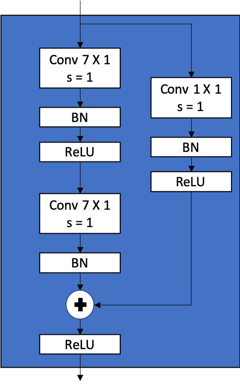
(a) Block

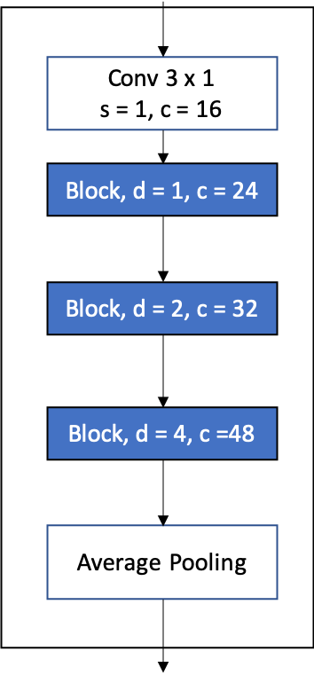
(b) TD-ResNet7

Figure 4: The proposed dilated time convolutional neural network for embedding.

4 Few-Shot Google Speech Command Dataset

Google’s Speech Commands dataset [18] has been used previously [5, 9] for keyword spotting problem. The dataset has a total of 35 keywords and contains multiple utterances of each keyword by multiple speakers. Each utterance is stored as a one-second (or less) WAVE format file, with the sample data encoded as linear 16-bit single-channel PCM values, at a 16 kHz rate. We curate a FS-KWS dataset from this dataset by performing the following preprocessing steps:

Keywords	Speakers	Utterances
		Min	Max	Mean
Core
down	1465	1	14	2.44
zero	1450	1	13	2.59
seven	1450	1	11	2.53
nine	1443	1	12	2.51
five	1442	1	19	2.58
yes	1422	1	20	2.6
four	1421	1	14	2.39
left	1416	1	12	2.47
stop	1413	1	22	2.52
six	1411	1	14	2.55
right	1409	1	15	2.45
on	1403	1	19	2.47
three	1401	1	11	2.43
off	1387	1	16	2.47
dog	1385	1	5	1.31
marvin	1378	1	6	1.33
one	1376	1	12	2.54
go	1372	1	12	2.53
no	1368	1	18	2.59
two	1367	1	15	2.58
eight	1358	1	15	2.53
house	1357	1	5	1.35
wow	1336	1	5	1.35
happy	1332	1	7	1.33
bird	1315	1	7	1.34
cat	1300	1	5	1.32
up	1291	1	17	2.53
sheila	1291	1	6	1.36
bed	1257	1	6	1.34
tree	1062	1	6	1.39
Unknown
visual	412	1	7	3.57
forward	397	1	10	3.66
backward	396	1	23	3.93
follow	387	1	11	3.76
learn	386	1	24	3.69

Table 1: Keyword Statistics

1. Filtering: We filter out all the utterances which are less than one second. This ensures the consistency of the output MFCC feature matrix obtained from each audio file.

2. Grouping: To train our KWS system to detect if an input query is an unknown keyword (not present in $S$), we group our keywords into two categories: Core and Unknown. Keywords having more than 1000 speakers are considered as core words and the rest are put in the category of unknown words.

3. Balancing: Next, we balance the dataset so that all keywords in a group have the same number of samples. As a result, we have 30 core keywords each with 1062 samples and 5 unknown keywords each with 386 samples and where all samples for a particular keyword come from a different speaker.

4. Splitting: (a) Core Keywords. They are randomly split into 20, 5, and 5 sets for training, validation, and testing respectively. Note that here the splits do not have any classes (keywords) in common. (b) Unknown Keywords. They are used for detecting negative inputs. Since we have only 5 keywords in an unknown category, we utilize them in all three phases of training, validation, and testing. For each keyword in the unknown category, 60% of its samples are used in training, 20% for validation, and 20% for testing. Note that in this case, all the training, validation, and test phases use the same 5 keywords as an unknown class but the samples are still from different speakers.

5. Mixing Background Noise: The original speech commands dataset [18] comes with a collection of sounds (6 WAVE files) that can be mixed with one-second utterances of keywords to simulate background noise. Following [20] implementation of mixing background noise, small snippets of these files are chosen at random and mixed at a low volume into audio samples during training. The loudness is also chosen randomly, and controlled by a hyper-parameter as a proportion where 0 is silence, and 1 is full volume. In our experiments, we set background volume to 0.1 and conduct experiments with both the presence and absence of background noise.

6. Detecting Silence: Apart from core classes and unknown class, we curate another class silence to detect the absence of keywords. Again following [20] implementation, we randomly sample 1000 one-second long sections of data from background sounds. Since there is never complete silence in real environments, we have to supply examples with quiet and irrelevant audio. We conduct experiments in both the presence and absence of samples from silence class.

We provide a script to synthesize this Few-Shot Speech Command dataset at our repository .

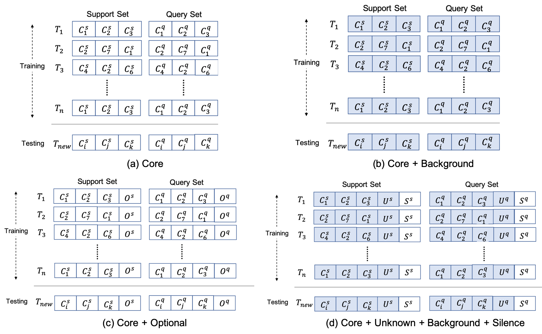
Figure 5: Training Cases demonstrated for 3-Way FS-KWS. (a) Core: In each task $T_{i}$, 3 Core classes are randomly sampled from $D_{train}$. Then for each Core class $C_{n}$, s support examples $C_{n}^{s}$ and q query examples $C_{n}^{q}$ are sampled (different from support examples). For testing, a new task $T_{new}$ is constructed which contains new classes $C_{i},C_{j},C_{k}$ sampled from $D_{test}$. (b) Core + Background: Here each keyword sample is mixed with background noise. (c) Core + Optional: An optional class (O) is present along with Core classes both during training and testing. (d) Core + Unknown + Background + Silence: Two optional classes i.e. Unknown (U) and Silence (S) are present and also the samples are mixed with background noise. (Note: In our experiments, the position of optional classes in (c) and (d) is random and not always at the last position as presented in this figure)

5 Experiments

5.1 Training

To test the effectiveness of our approach, we divide our experiments in four cases (Figure 5):

1. Core - Pure Keyword Detection: Both during training and testing, the keyword samples in the support ($S$) and query ($Q$) sets are from core keywords and without any background noise.

2. Core + Background: Same as (a), except the keyword samples are now mixed with random background noise.

3. Core + Optional: To account for scenarios when the input query is not from any of the keywords present in the provided support set or when there is simply no input, we train and test in presence of an optional class. This optional class is unknown keywords when we want to detect negatives and is silence when we want to detect the absence of any spoken keywords.

4. Core + Unknown + Silence + Background: Samples from both the optional classes i.e, Unknown and Silence are present and are also mixed with background noise. This case simulates more realistic scenarios when input is often mixed with background noise and could be an unknown word or just silence.

In each of the above cases, we train and test in a $N$-way $K$-shot manner where $N$ refers to the number of core classes and $K$ refers to the number of training examples per class in each episode as explained in Section 3. In cases where an optional class (Silence or Unknown) is used, we add $K$ support examples for the optional class in the support sets both during training and testing. We perform episodic training as suggested in [14] and train all our models for 200 epochs where each epoch has 200 training episodes and 100 validation (test) episodes. We use SGD with Adam [21] and an initial learning rate of $10^{-3}$ and cut the learning rate in half every 20 epochs. We conduct experiments with $N=\{2,4\}$ and $K=\{1,5\}$ for all the mentioned cases. The model is trained on the loss computed from 5 queries per class in each episode and evaluated more strictly with 15 queries per class during testing.

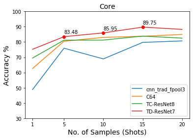
(a) Core

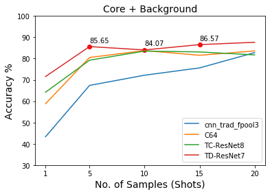
(b) Core + Background

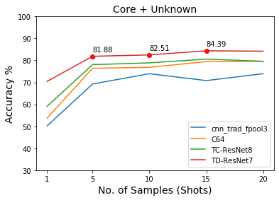
(c) Core + Unknown

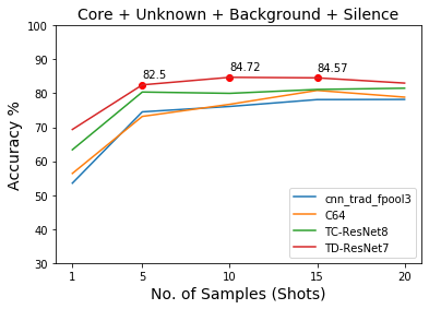
(d) Core + Unknown + Background + Silence

Figure 6: Comparing test accuracy of embedding network architectures on 4-way FS-KWS as we increase the number of support examples. The results are presented for all the four cases mentioned in section 5.1

5.2 Baselines

As we formulate and propose a new FS-KWS problem, there is a lack of prior research and standard FS-KWS dataset. Thus, to show the effectiveness of the proposed framework, we employ three different existing architectures as embedding network in our FS-KWS framework to examine the performance of the proposed approach. Following are the baseline embedding networks:

• cnn_trad_fpool3 [3] was originally proposed for KWS problem. It has two convolutional layers followed by a linear, a dense, and a softmax layer. We use the output of the dense layer as network embeddings.

• C64 [14] is the original 4-layer CNN used in Prototypical Networks for doing few-shot image classification on miniImageNet [13].

• TC-ResNet8 [9] has demonstrated great results on KWS. We remove the last fully connected and softmax layer and use the remaining architecture as our embedding network in FS-KWS framework.

5.3 Results

Table 2 lists the results for the three baselines and our proposed architecture on experiments mentioned in Section 5.1. Given a new 2-way-5-shot KWS task with keywords not seen during the training, our TD-ResNet7 model can classify an input query with $\sim$94% accuracy with the proposed FW-KWS pipeline. This is not even feasible with classical deep learning solutions withou FS-KWS formulation.

The TD-ResNet7 architecture also outperforms all the existing baselines architectures on all the test cases except in (b) Core + Background where the performance of TC-ResNet8 on 2-way 5-shot KWS is slightly better but the difference is not significant ($p=0.36$ while ANOVA for others presents $p\ll 0.05$). These results are illustrated in Figure 6. As we increase the number of shots (samples per class), the overall performance improves for all architectures, yet the TD-ResNet7 architecture consistently outperforms other baselines. All the accuracy results are averaged over 100 test episodes and are reported with 95% confidence intervals.

Case	Embedding Network	2-way Acc.		4-way Acc.
		1-shot	5-shot	1-shot	5-shot
core	cnn_trad_fpool3	69.23 $\pm$ 0.03	87.07 $\pm$ 0.02	48.83 $\pm$ 0.02	75.93 $\pm$ 0.01
	C64	77.20 $\pm$ 0.03	89.97 $\pm$ 0.02	62.63 $\pm$ 0.02	80.48 $\pm$ 0.01
	TC-ResNet8	82.70 $\pm$ 0.03	89.00 $\pm$ 0.02	69.47 $\pm$ 0.02	81.20 $\pm$ 0.01
	TD-ResNet7 (ours)	85.43 $\pm$ 0.03	94.10 $\pm$ 0.01	75.22 $\pm$ 0.02	83.48 $\pm$ 0.02
core + background	cnn_trad_fpool3	69.53 $\pm$ 0.04	86.8 $\pm$ 0.02	43.3 $\pm$ 0.02	67.42 $\pm$ 0.01
	C64	78.30 $\pm$ 0.03	90.03 $\pm$ 0.02	58.83 $\pm$ 0.02	80.52 $\pm$ 0.01
	TC-ResNet8	77.40 $\pm$ 0.03	91.40 $\pm$ 0.02	64.23 $\pm$ 0.02	79.25 $\pm$ 0.01
	TD-ResNet7 (ours)	82.23 $\pm$ 0.03	91.00 $\pm$ 0.02	71.58 $\pm$ 0.02	85.65 $\pm$ 0.01
core + unknown	cnn_trad_fpool3	58.33 $\pm$ 0.03	78.36 $\pm$ 0.02	50.15 $\pm$ 0.02	69.25 $\pm$ 0.01
	C64	63.42 $\pm$ 0.03	78.47 $\pm$ 0.02	53.69 $\pm$ 0.02	76.43 $\pm$ 0.01
	TC-ResNet8	68.84 $\pm$ 0.03	80.49 $\pm$ 0.02	59.08 $\pm$ 0.02	78.07 $\pm$ 0.01
	TD-ResNet7 (ours)	77.24 $\pm$ 0.02	87.22 $\pm$ 0.01	70.45 $\pm$ 0.02	81.88 $\pm$ 0.01
core + unknown + background + silence	cnn_trad_fpool3	67.43 $\pm$ 0.02	82.32 $\pm$ 0.01	53.51 $\pm$ 0.02	74.54 $\pm$ 0.01
	C64	65.83 $\pm$ 0.02	81.15 $\pm$ 0.01	56.38 $\pm$ 0.01	73.20 $\pm$ 0.01
	TC-ResNet8	78.63 $\pm$ 0.02	85.98 $\pm$ 0.01	63.37 $\pm$ 0.02	80.39 $\pm$ 0.01
	TD-ResNet7 (ours)	82.77 $\pm$ 0.02	89.45 $\pm$ 0.01	69.34 $\pm$ 0.01	82.50 $\pm$ 0.01

Table 2: Performance comparison of different embedding networks when plugged into FS-KWS pipeline for 4 different cases.

6 Conclusion

In this work, we attempted to solve the keyword spotting problem using only limited samples from each keyword. We demonstrated that using prototypical networks with our proposed embedding model which uses temporal and dilated convolutions, can produce significant results with only few examples. We also synthesis and release a Few-Shot Google Speech command dataset for future research on Few-Shot Keyword Spotting.

References

- [1] P. Motlicek, F. Valente, and I. Szoke, “Improving acoustic based keyword spotting using lvcsr lattices,” in 2012 IEEE International Conference on Acoustics, Speech and Signal Processing (ICASSP), 2012, pp. 4413–4416.
- [2] D. Can and M. Saraclar, “Lattice indexing for spoken term detection,” IEEE Transactions on Audio, Speech, and Language Processing, vol. 19, no. 8, pp. 2338–2347, 2011.
- [3] T. N. Sainath and C. Parada, “Convolutional neural networks for small-footprint keyword spotting,” in Sixteenth Annual Conference of the International Speech Communication Association, 2015.
- [4] G. Chen, C. Parada, and G. Heigold, “Small-footprint keyword spotting using deep neural networks,” in 2014 IEEE International Conference on Acoustics, Speech and Signal Processing (ICASSP). IEEE, 2014, pp. 4087–4091.
- [5] Y. Zhang, N. Suda, L. Lai, and V. Chandra, “Hello edge: Keyword spotting on microcontrollers,” arXiv preprint arXiv:1711.07128, 2017.
- [6] R. Tang and J. Lin, “Deep residual learning for small-footprint keyword spotting,” in 2018 IEEE International Conference on Acoustics, Speech and Signal Processing (ICASSP). IEEE, 2018, pp. 5484–5488.
- [7] D. C. de Andrade, S. Leo, M. L. D. S. Viana, and C. Bernkopf, “A neural attention model for speech command recognition,” arXiv preprint arXiv:1808.08929, 2018.
- [8] Y. LeCun, L. Bottou, Y. Bengio, P. Haffner et al., “Gradient-based learning applied to document recognition,” Proceedings of the IEEE, vol. 86, no. 11, pp. 2278–2324, 1998.
- [9] S. Choi, S. Seo, B. Shin, H. Byun, M. Kersner, B. Kim, D. Kim, and S. Ha, “Temporal convolution for real-time keyword spotting on mobile devices,” arXiv preprint arXiv:1904.03814, 2019.
- [10] A. Coucke, M. Chlieh, T. Gisselbrecht, D. Leroy, M. Poumeyrol, and T. Lavril, “Efficient keyword spotting using dilated convolutions and gating,” in ICASSP 2019-2019 IEEE International Conference on Acoustics, Speech and Signal Processing (ICASSP). IEEE, 2019, pp. 6351–6355.
- [11] W.-Y. Chen, Y.-C. Liu, Z. Kira, Y.-C. F. Wang, and J.-B. Huang, “A closer look at few-shot classification,” ArXiv, vol. abs/1904.04232, 2019.
- [12] G. Koch, R. Zemel, and R. Salakhutdinov, “Siamese neural networks for one-shot image recognition,” in ICML deep learning workshop, vol. 2, 2015.
- [13] O. Vinyals, C. Blundell, T. P. Lillicrap, K. Kavukcuoglu, and D. Wierstra, “Matching networks for one shot learning,” in NIPS, 2016.
- [14] J. Snell, K. Swersky, and R. Zemel, “Prototypical networks for few-shot learning,” in Advances in Neural Information Processing Systems, 2017, pp. 4077–4087.
- [15] S. Ravi and H. Larochelle, “Optimization as a model for few-shot learning,” in ICLR, 2017.
- [16] C. Finn, P. Abbeel, and S. Levine, “Model-agnostic meta-learning for fast adaptation of deep networks,” in ICML, 2017.
- [17] Y. Chen, T. Ko, L. Shang, X. Chen, X. Jiang, and Q. Li, “Meta learning for few-shot keyword spotting,” arXiv preprint arXiv:1812.10233, 2018.
- [18] P. Warden, “Speech commands: A dataset for limited-vocabulary speech recognition,” arXiv preprint arXiv:1804.03209, 2018.
- [19] J. S. Bridle, “Probabilistic interpretation of feedforward classification network outputs, with relationships to statistical pattern recognition,” in Neurocomputing. Springer, 1990, pp. 227–236.
- [20] P. Warden, Launching the speech commands dataset., 2017. [Online]. Available: https://ai.googleblog.com/2017/08/launching-speech-commands-dataset.html
- [21] D. P. Kingma and J. Ba, “Adam: A method for stochastic optimization,” arXiv preprint arXiv:1412.6980, 2014.