Abstract

We compute families of spherically symmetric neutron-star models in two-derivative scalar-tensor theories of gravity with a massive scalar field. The numerical approach we present allows us to compute the resulting spacetimes out to infinite radius using a relaxation algorithm on a compactified grid. We discuss the structure of the weakly and strongly scalarized branches of neutron-star models thus obtained and their dependence on the linear and quadratic coupling parameters $\alpha_{0}$, $\beta_{0}$ between the scalar and tensor sectors of the theory, as well as the scalar mass $\mu$. For highly negative values of $\beta_{0}$, we encounter configurations resembling a “gravitational atom”, consisting of a highly compact baryon star surrounded by a scalar cloud. A stability analysis based on binding-energy calculations suggests that these configurations are unstable and we expect them to migrate to models with radially decreasing baryon density and scalar field strength.

xx 1 5 Received: date; Accepted: date; Published: date Structure of neutron stars in massive scalar-tensor gravity Roxana Rosca-Mead¹ , Christopher J. Moore² , Ulrich Sperhake^1,3 , Michalis Agathos^1,4 and Davide Gerosa² Roxana Rosca-Mead, Christopher J. Moore, Ulrich Sperhake, Michalis Agathos and Davide Gerosa Correspondence: rr417@cam.ac.uk (R.R)

1 Introduction

Ever since its formulation in 1915, Einstein’s general relativity (GR) has been a tremendously successful theory of gravity, combining mathematical elegance with enormous predictive power. Phenomena ranging from Mercury’s perihelion precession to the formation of black holes (BHs), the generation of gravitational waves and the big bang, find a mathematical description within this single theory. A wide range of lab-based experiments, solar-system tests and observations of astronomical phenomena have systematically scrutinized the accuracy of the theory’s predictions and unanimously seen GR passing these tests with flying colors Will (2014). With the advent of gravitational-wave (GW) astronomy, marked by the detection of GW150914 by LIGO Abbott et al. (2016a), new tests of GR have become possible in spacetime regions with strong and dynamical gravitational fields and sources moving at relativistic velocities. Once again, all GW observations so far are compatible with GR Abbott et al. (2016b, 2017, 2019a, 2019b); Yunes et al. (2016).

Notwithstanding GR’s success, the search for possible alternative theories of gravity has for many decades been a highly active area of research Clifton et al. (2012); Will (2014); Berti et al. (2015); Barack et al. (2019); Olmo et al. (2019); Capozziello et al. (2019), motivated by important theoretical considerations, such as the incompatibility of GR with quantum theory at a fundamental level, as well as open questions in observational astronomy and cosmology. Astronomical observations of galactic rotation curves, micro-lensing, primordial nucleosynthesis or the accelerated expansion of the universe cannot be explained in GR without evoking dark matter and dark energy, enigmatic entities beyond the standard model of particles; see e.g. Freese (2009); Novosyadlyj et al. (2013).

Alternatively to either the dark-matter or dark-energy hypotheses, we may consider modifications in the laws of gravity; just in the same way GR explained Mercury’s anomalous perihelion precession in terms of modifications of the then prevailing Newtonian laws of gravity. Modifications of GR may also overcome one of the most important theoretical concerns about Einstein’s theory, its nonrenormalizability in quantum theory terms Hamber (2009). For a theory as well established as GR, however, the quest for modifications faces an obvious difficulty; the longstanding success of the old theory suggests that modifications either be extremely weak or become measurable only under new, in some sense extreme, conditions. Quite remarkably, however, this conclusion is not quite correct: nonperturbative effects of an alternative theory of gravity may lead to order-of-unity deviations from GR even if departures at linearized level are small. The prototypical example of this phenomenon is the spontaneous scalarization of neutron stars (NSs) Lasky (2015); Özel and Freire (2016) in scalar-tensor (ST) theory of gravity discovered by Damour and Esposito-Farèse in 1993 Damour and Esposito-Farese (1993). Here, the additional degree of freedom – in the form of the scalar field – allows for additional families of solutions describing stars in equilibrium. Moreover, these new families of solutions may appear “abruptly”, in a manner akin to phase-transitions, as one varies certain parameters of the theory or the star’s density profile. In the case of compact stars in ST gravity, the new solutions consist of stars with strong scalar-field profiles, as opposed to the GR-like models with negligible or zero scalar field. Often, the new scalarized configurations are energetically favored over their GR-like counterparts (assuming equal baryon mass or number), so that they represent the expected endpoints of dynamical scenarios.

Spontaenous scalarization bears a qualitative resemblence to other effects known in physics; Damour and Esposito-Farèse have highlighted its analogy to the spontaneous magnetization of ferromagnets Damour and Esposito-Farese (1996) and later studies have interpreted its onset in terms of catastrophe theory Harada (1998) or a tachyonic instability Ramazanoğlu and Pretorius (2016). Originally, spontaneous scalarization has been identified for spherically symmetric NS models in a class of massless ST theories sometimes refered to as Bergmann-Wagoner Bergmann (1968); Wagoner (1970) theories; these complement the metric sector of GR with a single scalar field, are governed by second-order covariant field equations at most linear in second and quadratic in first derivatives, and obey the weak equivalence principle. The phenomenon has by now been demonstrated to occur over a wide range of configurations and also in other theoretical frameworks Andreou et al. (2019); Ventagli et al. (2020). Analogous phenomena occur in many scenarios involving fields non-minimally coupled to a spacetime metric. Examples include scalarized BHs in theories with Gauss-Bonnet coupling Silva et al. (2018); Doneva and Yazadjiev (2018), universal horizons in Lorentz violating gravity theories Barausse et al. (2011) and the spotaneous vectorization or tensorization of compact stars in modified gravity Ramazanoğlu (2017); Annulli et al. (2019); Ramazanoğlu (2019).

Numerous studies have demonstrated that spontaneous scalarization features as prominently in rotating NS models, either in the slow-rotation limit Sotani (2012); Pani and Berti (2014); Silva et al. (2015); Yazadjiev et al. (2016); Altaha Motahar et al. (2017); Staykov et al. (2018), for fast rotation Doneva et al. (2013, 2014), or with differential rotation Doneva et al. (2018). Spontaneous scalarization has also been found a robust phenomenon under variations of the equation of state (EOS) Ramazanoğlu and Pretorius (2016); Altaha Motahar et al. (2017); Sotani and Kokkotas (2017); Rezaei and Dezdarani (2019); Anderson and Yunes (2019). While quantitative differences occur, the phenomenon as such appears to be ubiquitous and also preserve the approximate EOS universality of the relation between the moment of inertia $I$ and the quadrupole moment $Q$ known from GR Doneva et al. (2014); Pani and Berti (2014) and the inertia vs. compactness universality Altaha Motahar et al. (2017).

Numerical calculations find that the families of scalarized NSs can have larger maximal masses than the corresponding GR solutions Damour and Esposito-Farese (1993); Ramazanoğlu and Pretorius (2016); Morisaki and Suyama (2017); Doneva et al. (2018). Often this is accompanied with an even stronger increase in the NS radius, so that the maximum compactness of NSs in ST gravity is smaller than in GR Sotani and Kokkotas (2018). These findings suggest that the scalar field may effectively stiffen the equation of state and thus counteract the normal gravitational pull. This effect, does not appear to be generic, however, but rather depends on details of the matter sources. A generalization of the Buchdahl limit Tsuchida et al. (1998) has found that compactness above the Buchdahl limit is possible in ST theory, but only if the energy density $\rho$ and pressure $p$ satisfy $\rho<3p$. Sotani and Kokkotas Sotani and Kokkotas (2017) find that the maximum NS mass is larger in ST theory than in GR for sufficiently small sound speeds in the core, but that the reverse holds if this velocity exceeds 0.79 of the speed of light. In light of the recent discovery by LIGO and Virgo of the compact binary GW190814, whose light component’s mass likely falls in the so-called mass gap between NS and BHs Abbott et al. (2020), it is worth noting that massive ST gravity allows for the possibility of such objects being strongly scalarized NSs.

The presence or absence of the spontaneous scalarization phenomenon is largely determined by the quadratic coupling parameter $\beta_{0}$ between the scalar and tensor sectors of the theory; cf. Eq.(4) below. Strongly scalarized NS models are found for $\beta_{0}\lesssim-4.35$ and this threshold has been found remarkably robust against variations of other parameters such as the EOS; see e.g. Novak (1998); Pani and Berti (2014). In a series of studies, however, Mendes and collaborators Mendes et al. (2014); Mendes (2015); Mendes and Ortiz (2016) have demonstrated that strongly scalarized solutions can also be obtained for positive values of $\beta_{0}$ provided there exist stable equilibrium solutions for matter fields in the GR limit where the trace $T$ of the energy-momentum tensor acquires positive values. This can be understood, for instance, in terms of the tachyonic instability by noticing that the scalar field is sourced by a term $\propto\beta_{0}T$; cf. Eq. (3) in Ref. Ramazanoğlu and Pretorius (2016). This $\beta_{0}>0$ scenario has been explored in time evolutions of NSs close to the upper NS mass limit in Ref. Palenzuela and Liebling (2016). These simulations demonstrate an instability of the star to collapse for large $\beta_{0}$ of $\mathcal{O}(10^{2})$, suggesting an upper bound on the parameter $\beta_{0}$.

Massless ST theories of gravity have by now been significantly constrained – not least of all because of the large magnitude of the spontaneous scalarization effect – by the Cassini mission Bertotti et al. (2003), Lunar Laser Ranging Williams et al. (2009), binary pulsar observations Wex (2014) and gravitational wave (GW) observations with LIGO-Virgo Yunes et al. (2016). While spontaneous scalarization has been seen to occur in dynamical evolutions in massless ST theory, either for the gravitational collapse of single stars Novak (1998, 1998); Novak and Ibanez (2000); Gerosa et al. (2016) or the merger of binary NSs Barausse et al. (2013); Palenzuela et al. (2014); Shibata et al. (2014), the most recent constraints on $\beta_{0}$ severely limit the magnitude of the resulting GW signals and, thus, make it difficult to constrain this theory further with GW observations.

In the context of this work, the most important extension of the scalarization phenomenon is the inclusion of a non-zero scalar mass. This is because the above constraints only apply to ST theories with a scalar mass parameter $\mu\lesssim 10^{-16}\,{\rm eV}$. Otherwise, the Compton wavelength $\lambda_{c}=(2\pi\hbar)/(\mu c)$ is smaller than the distance between the objects involved in the systems under consideration and, hence, the scalar contribution to the objects’ interaction is suppressed. GW observations, on the other hand, provide exquisite constraints on dispersion which in turn can be interpreted as a constraint on the graviton mass, but this does not apply to radiation in the scalar sector. In consequence, massive ST theory remains compatible with present observations over much of its parameter space.

Motivated by this realization, many recent studies have explored spontaneous scalarization in massive ST gravity. Computations of stationary models have confirmed that the spontaneous scalarization phenomenon persists under the inclusion of a mass term in the scalar potential Chen et al. (2015); Doneva and Yazadjiev (2016); Yazadjiev et al. (2016); Ramazanoğlu (2017); Morisaki and Suyama (2017). A non-zero scalar mass $\mu>0$ does, however, dramatically affect the GW signals generated in stellar collapse in ST gravity through dispersion. A Fourier mode with frequency $\omega$ propagates at group velocity $v_{g}=\sqrt{1-\omega_{*}^{2}/\omega^{2}}$, $\omega_{*}=c^{2}\mu/\hbar$, so that high-frequencies reach a detector first with lower frequencies arriving later, so the signal acquires an inverse-chirp or howl character. Furthermore these signals get extremely stretched out and become approximately monochromatic (in the sense that the frequency changes by very little over one period; $\mathrm{d}f/\mathrm{dt}\ll f^{2}$), can reach considerable amplitude for sufficiently negative $\beta_{0}$ and may last for years or even centuries for scalar masses $\mu\lesssim 10^{-12}~{}{\rm eV}$ Sperhake et al. (2017); Rosca-Mead et al. (2020); Geng et al. (2020). While the inclusion of self-interaction terms may reduce the degree of scalarization and the amplitude of the scalar GWs Cheong and Li (2019); Staykov et al. (2018), this requires considerable finetuning of the scalar potential parameters Rosca-Mead et al. (2019).

In this work, we focus on spherically symmetric, static NS models in the framework of Bergmann-Wagoner ST theory with massive scalar fields. The main purpose of our study is two-fold. First, to introduce a numerical scheme that enables us to compute these stellar models over the entire spatial domain, all the way out to infinity, while maintaining complete control over exponentially diverging solutions. Second, to present an in-depth analysis of the structure of the different solution branches and their dependence on the parameters of the ST theory. We begin this discussion in Sec. 2 with a review of the field equations governing the stars. In Sec. 3, we describe the numerical framework used for our computations. Our results on the structure of NS solutions in massive ST gravity are presented in Sec. 4 and we conclude in Sec. 5.

2 Formalism

The Bergmann-Wagoner class of ST theories, i.e. theories involving a single scalar field that are governed by two-derivative, covariant field equations and obey the weak equivalence principle, can be described in terms of the action Fujii and Maeda (2007)

$$S_{J}=\int dx^{4}\sqrt{-g}\left[\frac{F(\phi)}{16\pi G}R-\frac{1}{2}Z(\phi)g^{\mu\nu}(\partial_{\mu}\phi)(\partial_{\nu}\phi)-W(\phi)\right]+S_{m}(\psi_{m},g_{\mu\nu})\,.$$ (1)

Here, $\psi_{m}$ collectively denotes the matter fields and $S_{m}$ represents their coupling to the spacetime geometry of the physical or Jordan metric $g_{\mu\nu}$ with determinant $g$ and Ricci scalar $R$. The functions $F(\phi)$ and $Z(\phi)$ encapsulate the nonminimal coupling of the scalar field $\phi$ to the metric sector, and $V(\phi)$ is the potential function. As we shall see shortly, the function $Z$ can be eliminated through an appropriate redefinition and is therefore often set to unity in the literature; see e.g. Salgado (2006).

This class of theories is conveniently described in the so-called Einstein frame, obtained from the physical or Jordan frame through a conformal transformation of the metric and a redefinition of the scalar degree of freedom and its potential,

$$g_{\alpha\beta}=\frac{1}{F}\bar{g}_{\alpha\beta},~{}~{}~{}~{}~{}~{}~{}~{}~{}~{}\frac{\partial\varphi}{\partial\phi}=\sqrt{\frac{3}{4}\frac{F_{,\phi}(\phi)^{2}}{F(\phi)^{2}}+\frac{4\pi Z(\phi)}{F(\phi)}}\,,~{}~{}~{}~{}~{}~{}~{}~{}~{}~{}V(\varphi)=\frac{4\pi W(\phi)}{F(\phi)^{2}}\,,$$ (2)

where $F_{,\phi}=dF/d\phi$. In terms of these new functions, the action (1) becomes

$$S_{E}=\frac{1}{16\pi G}\int dx^{4}\sqrt{-\bar{g}}\left[\bar{R}-2\bar{g}^{\mu\nu}(\partial_{\mu}\varphi)(\partial_{\nu}\varphi)-4V(\varphi)\right]+S_{m}\left[\psi_{m},\frac{\bar{g}_{\mu\nu}}{F(\varphi)}\right]\,,$$ (3)

where an overbar distinguishes tensors in the Einstein frame from their Jordan counterparts. Henceforth, we use natural units where $c=G=1$, unless stated otherwise.

By transforming to the Einstein frame, we have eliminated the function $Z$. The equivalence (or lack thereof) of the Einstein and Jordan frame formulations has been the subject of a long standing debate (see e.g. Faraoni and Gunzig (1999); Salgado et al. (2008); Geng et al. (2020) and references therein). Without entering this debate here, we merely note the extra freedom that the function $Z$ introduces to the transformation (2) between the frames and henceforth follow the recommendation of Ref. Faraoni and Gunzig (1999) and work in the Einstein frame.

To complete the description of the gravitational theory we must specify the remaining free functions $F$ and $V$. Following most previous studies in the literature, we write the conformal factor as

$$F(\varphi)=e^{-2\alpha_{0}\varphi-\beta_{0}\varphi^{2}}\,,$$ (4)

and take as our potential function the quadratic function

$$V(\varphi)=\frac{\mu^{2}\varphi^{2}}{2\hbar^{2}}\,,$$ (5)

which describes a non-self-interacting scalar field of mass $\mu$.

The field equations obtained by varying the Einstein action (3) with respect to $\bar{g}_{\alpha\beta}$, $\varphi$ are given by

$$\bar{R}_{\alpha\beta}-\frac{1}{2}\bar{g}_{\alpha\beta}\bar{R} = 2\partial_{\alpha}\varphi\partial_{\beta}\varphi-\bar{g}_{\alpha\beta}\bar{g}^{\mu\nu}\partial_{\mu}\varphi\partial_{\nu}\varphi+8\pi\bar{T}_{\alpha\beta}-2V\bar{g}_{\alpha\beta},$$ (6)

$$\bar{\Box}\varphi = 2\pi\frac{F_{,\varphi}}{F}\bar{T}+V_{,\varphi}\,,$$ (7)

with the energy momentum tensor

$$\bar{T}^{\alpha\beta}=\frac{2}{\sqrt{-\bar{g}}}\frac{\delta S_{m}}{\delta\bar{g}_{\alpha\beta}}=\frac{1}{{F(\varphi)}^{3}}\frac{2}{\sqrt{-g}}\frac{\delta S_{m}}{\delta g_{\alpha\beta}}=\frac{1}{{F(\varphi)}^{3}}T^{\alpha\beta}\,,$$ (8)

for which the Bianchi identity now implies the following conservation law

$$\bar{\nabla}_{\mu}\bar{T}^{\mu\alpha}=-\frac{1}{2}\frac{F_{,\varphi}}{F}\bar{T}\bar{g}^{\alpha\mu}\bar{\nabla}_{\mu}\varphi\,.$$ (9)

From now on, we restrict our attention to spherically symmetric, time independent stellar models. More specifically, we employ polar slicing and radial gauge in the Einstein frame, so that the line element is of the form

$$\mathrm{d}\bar{s}^{2}=\bar{g}_{\mu\nu}\mathrm{d}x^{\mu}\mathrm{d}x^{\nu}=-F\,\alpha^{2}\mathrm{d}t^{2}+F\,X^{2}\mathrm{d}r^{2}+r^{2}\mathrm{d}\Omega^{2}\,,$$ (10)

where $\alpha$ and $X$ as well as the scalar field $\varphi$ are functions of the radius $r$, and $\mathrm{d}\Omega^{2}$ denotes the standard line element on the unit 2-sphere. It is furthermore common practice to introduce the gravitational potential $\Phi$ and mass function $m$ according to

$$F\,\alpha^{2}=e^{2\Phi},~{}~{}~{}~{}~{}F\,X^{2}=\left(1-\frac{2m}{r}\right)^{-1}\,.$$ (11)

In this work we explore the behaviour of NSs in equilibrium and model their matter as a perfect fluid at zero temperature; the temperature of NS interiors in equilibrium, despite being of order $10^{6}\,\mathrm{K}$, is well below the Fermi temperature $\mathcal{O}(10^{11})\,\mathrm{K}$ of matter at nuclear densities. The energy momentum tensor is then given in terms of the baryon density $\rho(r)$, the specific enthalphy $h(r)$ and the pressure $P(r)$ by

$$\bar{T}_{\alpha\beta}=\frac{1}{F}T_{\alpha\beta}=\frac{1}{F}\left(\rho hu_{\alpha}u_{\beta}+Pg_{\alpha\beta}\right)\,,$$

$$\text{with}~{}~{}~{}~{}~{}~{}~{}~{}u^{\alpha}=\left[\alpha^{-1},~{}0,~{}0,~{}0\right]\,,~{}~{}~{}~{}~{}~{}~{}~{}h=1+\epsilon+\frac{P}{\rho}\,,$$ (12)

and where $\epsilon$ is the specific internal energy. Inserting the Einstein frame metric (10) and the energy momentum tensor (12) into the field equations (6)-(9), we obtain the set of differential equations

$$\partial_{r}\Phi = \frac{FX^{2}-1}{2r}+\frac{4\pi rPX^{2}}{F}+\frac{rX^{2}\eta^{2}}{2}-WrX^{2}F\,,$$ (13)

$$\partial_{r}X = \frac{4\pi rX^{3}}{F}(\rho h-P)+\frac{rX^{3}\eta^{2}}{2}\,,-\frac{X^{3}F}{2r}+\frac{X}{2r}-\frac{F_{,\varphi}X^{2}\eta}{2F}+X^{3}FWr\,,$$ (14)

$$\partial_{r}P = -\rho hFX^{2}\left(\frac{m}{r^{2}}+4\pi r\frac{P}{F^{2}}+\frac{r}{2F}{\eta}^{2}-rW\right)+\rho h\frac{F_{,\varphi}}{2F}X\eta\,,$$ (15)

$$\partial_{r}\varphi = X\eta\,,$$ (16)

$$\partial_{r}\eta = -\frac{3\eta}{2r}-\frac{2\pi XF_{,\varphi}}{F^{2}}(\rho h-4P)-\frac{X^{2}\eta F}{2r}-\frac{4X^{2}\eta\pi rP}{F}-\frac{X^{2}\eta^{3}r}{2}$$ (17)

$$+\frac{X\eta^{2}F_{,\varphi}}{2F}+X^{2}\eta FWr+XF\partial_{\varphi}W\,.\,$$

In order to close this set of equations, we need to relate the pressure and internal energy to the baryon density. In this work, we use cold polytropic EOSs with exponent $\Gamma$,

$$P=K\rho^{\Gamma}\,,$$ (18)

The internal energy is then determined by the first law of thermodynamics $dE={~{}~{}\mathchar 22\relax\mkern-11.0mud}Q-pdV$ for adiabatic processes with ${~{}~{}\mathchar 22\relax\mkern-11.0mud}Q=0$. For a total baryon number $N$ and mass per baryon $m_{b}$, the specific internal energy and baryon density are given by $\epsilon=E/(Nm_{b})$ and $\rho=m_{b}N/V$, respectively, and the first law results in

$$\epsilon=\frac{P}{(\Gamma-1)\rho}\,.$$ (19)

The set of equations (13)-(17) can then be solved subject to the boundary conditions

$$\text{at}~{}~{}r=0:~{}~{}~{}~{}\, \eta=0\,,~{}~{}~{}~{}~{}~{}~{}~{}~{}~{}~{}FX^{2}=1\,,$$

$$\text{at}~{}~{}r\rightarrow\infty:~{}~{} \Phi=0\,,~{}~{}~{}~{}~{}~{}~{}~{}~{}~{}\rho=0\,,~{}~{}~{}~{}~{}~{}~{}~{}~{}~{}\varphi=0\,.$$ (20)

The computation of solutions to this problem is complicated by three issues, which we list in increasing order of difficulty.

• The boundary conditions are specified at different locations of the domain, so that we have a two-point-boundary-value problem.

• For realistic values of the polytropic exponent $\Gamma$, the pressure will reach zero at a finite radius $R_{S}$; at this point, we need to match to an exterior solution with vanishing baryon density $\rho$.

• The asymptotic behaviour of the scalar field near infinity is determined by the scalar mass $\mu$ and is given by

  $$\lim_{r\rightarrow\infty}\varphi\sim A_{1}\frac{e^{-(\mu/\hbar)r}}{r}+A_{2}\frac{e^{(\mu/\hbar)r}}{r}\,,$$ (21)

  for constants $A_{1}$, $A_{2}$. We are only interested in bounded solutions with $\varphi\propto e^{-(\mu/\hbar)r}/r$. This exponential fall-off is responsible for the suppressed scalar contribution in the interaction of pulsar binaries in massive ST gravity and forms the key motivation for our study. From a purely numerical point of view, however, Eq. (21) creates a significant challenge. Numerical algorithms will pick up all possible modes of a solution – even if only through roundoff error.

We therefore seek an algorithm that provides us with explicit control over the asymptotic behaviour of our numerical solutions. In the next section, we will discuss how this can be achieved inside the more standard frameworks employed to address items (i) and (ii) of our above list.

3 Numerical framework

Numerical methods for solving two-point-boundary-value problems are well developed and fall into two main classes, shooting algorithms and relaxation schemes (including collocation methods) Press, William H. and Teukolsky, Saul A. and Vetterling, William T. and Flannery, Brian P. (1992) To the best of our knowledge, all literature on static NS models in ST gravity has employed shooting algorithms; see e.g. Ramazanoğlu and Pretorius (2016); Yazadjiev et al. (2016). This process integrates the differential equations from one end of the domain by supplementing the known boundary conditions at this point with appropriate trial values for the remaining variables. The resulting integration will typically not match the boundary conditions at the other end of the domain, but the degree of violation can be used, e.g. through a Newton-Raphson or a bisection method, to iteratively improve the trial values until all boundary conditions are satisfied within a user-specified threshold accuracy.

For the case of our system of differential equations (13)-(17) with boundary conditions (20), this would work as follows. We first note that the function $\Phi$ appears only in Eq. (13) and in the form of its spatial derivative. We can therefore set $\Phi(0)=0$ and add an arbitrary constant to match its boundary condition after having solved for all variables. Bearing in mind this freedom, we start the integration at the origin $r=0$ by selecting values for the central baryon density $\rho(0)$, the central scalar field amplitude $\varphi(0)$ and the metric function $\Phi(0)$, additionally to the known $\eta(0)=0$ and $X(0)=1/\sqrt{F(\varphi(0))}$. The integration will reach zero pressure at a finite $r$ which represents the NS radius. Beyond this radius, the integration continues setting $\rho=P=0$ in Eqs. (13)-(17). In principle this surmounts the issue (ii) mentioned in the previous section. We note, though, that $P=0$ is, in general, not realized on a grid point which adds a small discontinuity to the solution; the data on the outermost grid point inside the star and on the first point outside the star do not satisfy Eqs. (13)-(17). This discontinuity is typically not problematic, but we will see below how it can be simply eliminated in a relaxation approach. For a massless scalar field, it is even possible to analytically match the spacetime to an exterior vacuum metric; cf. Eqs. (8), (9) in Damour and Esposito-Farese (1993). Integration beyond the neutron star radius is not required and the trial value $\varphi(0)$ can be improved in accordance with the selected shooting algorithm.

Such an analytic matching is not known, however, for massive scalar fields. And now a more problematic issue arises as the integration is continued beyond the NS radius; no matter how accurate the central value $\varphi(0)$ has been chosen, the numerical solution will contain an exponentially growing contribution from the asymptotic behaviour (21) and eventually blow up exponentially. Worse, this blowup prevents us from improving our trial value $\varphi(0)$ through measuring the departure from the correct boundary condition at infinity; this departure is infinite and, hence, useless for numerical purposes. In shooting algorithms, this problem is circumvented by imposing the outer boundary conditions at a finite radius rather than infinity; cf. Sec. III A in Ramazanoğlu and Pretorius (2016).

While this method is still capable of generating accurate stellar models, a scheme covering the complete exterior and imposing the boundary conditions at infinity provides practical advantages besides the more rigorous boundary treatment. By extending all the way to infinity, our scheme can provide initial data for time evolutions on arbitrarily large computational domains (including compactified evolution schemes that incorporate spatial or null infinity) without resorting to adhoc procedures to extend results beyond the inevitably finite blow-up radius of shooting methods. We will also obtain a vacuum exterior that is matched to the NS interior on a grid point; in fact, the value of the NS surface, rather than the central density, will select the specific stellar model. Furthermore, the relaxation scheme provides an exceptionally elegant and simple way to implement the matching between the interior and exterior domain that we expect to be applicable to a wider range of problems, including extension to time evolutions.

For our method, we first introduce the NS radius $R_{S}$ as a free parameter. On the domain $r\in[0,R_{S}]$, we use the differential equations (13)-(17) with boundary conditions (20) for $\eta$ and $X$ at $r=0$; the condition $FX^{2}=1$ is formulated as an equation involving the unknown $\varphi(0)$. In the exterior, we introduce a compactified radial coordinate

$$y=\frac{1}{r}\,,$$ (22)

set $\rho=P=0$, and introduce rescaled variables

$$\sigma=\varphi e^{(\mu/\hbar)r}\,,~{}~{}~{}~{}~{}~{}~{}~{}~{}~{}\kappa=-\eta e^{(\mu/\hbar)r}\,.$$ (23)

By factoring the exponential dependence into our scalar field variables, we ensure that regular solutions $\sigma$ and $\kappa$ asymptote towards a $\propto y$ dependence at $y=0$. We find this step crucial in achieving convergence of our relaxation scheme which struggles with the exponential fall-off of $\varphi$ and $\eta$ but copes smoothly with the benign linear behaviour of the rescaled $\sigma$ and $\kappa$. We also notice a minor (but not crucial) improvement in the speed of convergence when switching from $X$ to the mass function $m$ of Eq. (11) and hence use the set of variables $\Phi,~{}m,~{}\sigma,~{}\kappa$ in the exterior. The differential equations in the exterior domain $y\in[0,y_{\rm S}]$, $y_{\rm S}=1/R_{\rm S}$, thus become

$$\partial_{y}\Phi = -\frac{m}{1-2my}-\frac{1}{2\left(1-2my\right)y^{3}e^{2\mu/y}}\left(\frac{\kappa^{2}}{F}-\mu^{2}\sigma^{2}\right)\,,$$ (24)

$$\partial_{y}m = -\frac{1}{2y^{4}e^{2\mu/y}}\left(\frac{\kappa^{2}}{F}-\mu^{2}\sigma^{2}\right)\,,$$ (25)

$$\partial_{y}\sigma = \frac{X\kappa-\mu\sigma}{y^{2}}\,,$$ (26)

$$\partial_{y}\kappa = -\kappa\partial_{y}\Phi+\frac{FX\mu^{2}\sigma+\kappa\left(2y-\mu\right)}{y^{2}}+\frac{X\kappa^{2}}{2y^{2}}\frac{F_{,\varphi}}{F}\,,$$ (27)

and the matching conditions imposed at the surface of the NS are given by

$$\Phi(y_{\rm S}) = \Phi(R_{\rm S})\,,$$

$$m(y_{\rm S}) = \left[\frac{r}{2}\left(1-\frac{1}{FX^{2}}\right)\right]_{r=R_{\rm S}}\,,$$

$$\sigma(y_{\rm S}) = \varphi(R_{\rm S})e^{(\mu/\hbar)R_{\rm S}}\,,$$

$$\kappa(y_{\rm S}) = -\eta(R_{\rm S})e^{(\mu/\hbar)R_{\rm S}}\,.$$ (28)

We formally also use the trivial equation $\partial_{y}P=0$ in the exterior which allows us to use a constant number of five variables over the entire grid. This grid consists of $N$ grid points in the interior and $M$ points in the exterior. We discretize the differential equations using cell-centered second-order stencils which provides us with $5(N-1)$ algebraic equations in the interior and $5(M-1)$ equations in the exterior. The boundary conditions provide two further equations at $r=0$ and three further equations at $y=0$. The surface radius is represented twice on our grid, the outermost point $r=R_{\rm S}$ of the interior and the innermost point $y_{\rm S}$ of the exterior grid. The variables used on these points are related by the matching conditions (28) as well as the trivial $P(R_{\rm S})=P(y_{\rm S})=0$. In total, we thus have $5(N+M)$ non-linear algebraic equations for the $5(N+M)$ unknown values of the variables on the grid points. Given an initial guess, we can linearize the equations around this trial solution which leads to a matrix equation with block-diagonal structure that is readily inverted to improve the guess iteratively; we use the algorithm of Ref. Press, William H. and Teukolsky, Saul A. and Vetterling, William T. and Flannery, Brian P. (1992) and typically obtain convergence after about ten iterations. The initial guess is obtained by integrating Eqs. (13)-(17) up to $R_{\rm S}$, fixing $\sigma$ and $\kappa$ as linear functions $\propto y$ in the exterior and integrating Eqs. (24), (25) with these specified scalar sources. Note that in this calculation we set $\rho=P=0$ in the exterior irrespective of whether or not they have reached zero at $R_{\rm S}$; the discontinuity that may result at the matching point is removed in the ensuing relaxation process.

Even for modest resolutions such as $N=M=401$, this approach provides an accuracy of $O(10^{-4})$. All models discussed in the remainder of this paper have been computed with this code.

4 Results

4.1 Overall phenomenology

We start this section by defining the terminology and diagnostic quantities as well as providing a qualitative review of the different branches of static NS models encountered in massive ST gravity. We then explore in the following subsections in more detail the impact of the ST parameters $\alpha_{0}$, $\beta_{0}$ and $\mu$ on the structure of these branches.

In the following, we will use the term “family” for the set of all NS models obtained for fixed EOS and ST parameters $\alpha_{0}$, $\beta_{0}$ and $\mu$. We will use the term “branch” to denote a subset of solutions of a family that share some specific property, for example strong scalarization. A family thus consists of one or more branches. In some cases, we find a branch to have the shape of a closed loop disconnected from other branches, and we also refer to such a branch as a “loop”. For reference, we note that the scalar mass $\mu$ introduces a Compton wavelength and characteristic frequency given by

$$\lambda_{C}=1.24\times 10^{6}\,\mathrm{km}~{}\left(\frac{\mu}{10^{-15}\,\mathrm{eV}}\right)^{-1}\,,~{}~{}~{}~{}~{}~{}~{}~{}~{}~{}f_{*}=\frac{\omega_{*}}{2\pi}=24.2\,\mathrm{Hz}~{}\left(\frac{\mu}{10^{-15}\,\mathrm{eV}}\right)^{-1}\,.$$ (29)

Unless stated otherwise, our numerical NS models in massive ST theory are computed with the polytropic EOS labelled “EOS1” in Ref. Novak (1998). Translated into our notation, we therefore compute the pressure and specific internal energy from the baryon density $\rho$ through Eqs. (18) and (19) with

$$K=1.543~{}\frac{\mathrm{cm}^{3\Gamma-1}}{\mathrm{g}^{\Gamma-1}\mathrm{s}},~{}~{}~{}~{}~{}~{}~{}~{}~{}~{}\Gamma=2.34\,.$$ (30)

The families of solutions thus obtained are conveniently represented in a mass-radius diagram. For this purpose, we define the total baryon mass $M_{b}$ as the volume integral of the baryon number density multiplied by the mass per baryon $m_{b}$. Translated into our baryon density $\rho=m_{b}n_{b}$, the expression becomes

$$M_{b}=m_{b}\int d^{3}x\sqrt{-g}n_{b}u^{t}=4\pi\int_{0}^{R_{S}}dr\left(r^{2}\frac{\rho}{F^{3/2}\sqrt{1-2m/r}}\right)\,.$$ (31)

The motivation for using the baryon mass, rather than the gravitational mass of Eq. (11), arises from the conservation of the baryon number; if we consider the possibility that a NS might migrate dynamically from one branch to another, we expect it to do so at constant $M_{b}$, whereas the binding energy and, hence, gravitational mass will, in general, change.

As in massless ST theories, all NS solutions can be classified as either weakly scalarized with scalar field profiles reaching a magnitude $\varphi\sim O(\alpha_{0})$ or strongly scalarized solutions where the scalar field reaches values $\varphi\sim O(1)$ Damour and Esposito-Farese (1993). In this work, we call these branches W (for weak) and S (for strong scalarization); see e. g. Fig. 1. The distinction between the two regimes naturally blurs for large values $\alpha_{0}=\mathcal{O}(1)$; in this work we consider only $\alpha_{0}\ll 1$ and thus retain a clear division between weakly and strongly scalarized NSs.

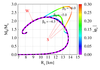
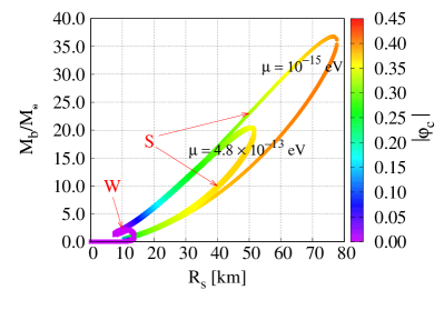
Figure 1: Branches of NS models are shown in the form of baryon-mass vs. radius ($M_{b}-R_{S}$) diagrams. Left: For fixed values $\alpha_{0}=10^{-4}$ and $\mu=4.8\times 10^{-13}\,\mathrm{eV}$, we plot the strongly scalarized branches obtained for selected values of $\beta_{0}$. For reference, the dashed black curve displays the solutions obtained in GR with $\alpha_{0}=\beta_{0}=0$. Right: Here we fix $\alpha_{0}=10^{-4}$ and a more extreme value of $\beta_{0}=-15$ and vary the scalar mass $\mu$; larger deviations from the GR structure are clearly visible in this case. In both panels the color scale measures the central value of $|\varphi|$ and the “S” and “W” label the strongly and weakly scalarized branches described in the text.

As is well known, the NS solutions in GR form a one-parameter family whose members can be characterized by its central density $\rho_{c}$ Shapiro and Teukolsky (1983). For the EOS (30), this leads to the black branch in the left panel of Fig. 1. In ST gravity, the introduction of a scalar field leads to additional branches of NS solutions with a non-vanishing scalar-field profile $\varphi(r)$. The shape of the extra branches depends on the values of the parameters $\alpha_{0}$, $\beta_{0}$ and $\mu$. In agreement with the literature Novak (1998), we observe strongly scalarized solutions if $\beta_{0}\lesssim-4.35$. These new branches are displayed in the left panel of Fig. 1 in terms of a color code that denotes the central scalar field amplitude. In contrast, the weakly scalarized solutions we obtain for $\beta_{0}\gtrsim-4.35$ have macroscopic properties that barely differ from those of the GR solutions and their branch would be indistinguishable from the GR family in the figure. For these cases, we have set $\alpha_{0}=10^{-4}$ and $\mu=4.8\times 10^{-13}\,\mathrm{eV}$. We now discuss in more detail how the solutions and their branches vary when the parameter values are changed.

4.2 Dependence on $\mu$

The variation of scalarized NS branches in massive ST theory has already been studied in Ref. Ramazanoğlu and Pretorius (2016) who generally observe that an increase in the scalar mass $\mu$ results in a weakening of the scalarization. By computing a sequence of models with equal gravitational or “Arnowitt-Deser-Misner” (ADM) Arnowitt et al. (2008) mass, they observe a monotonic decrease in the scalarization as the scalar mass is increased. Around $10^{-12}\,\mathrm{eV}$, their scalar profile drops to negligible levels when $\beta_{0}=-4.5$; cf. their Fig. 2. Our results exhibit a similar drop in scalarization. We illustrate this general behaviour by comparing the cases $\mu=10^{-15}\,\mathrm{eV}$ and $\mu=4.8\times 10^{-13}\,\mathrm{eV}$ in the right panel of Fig. 1; the color code of the branches represents the central scalar field amplitude and displays lower values for the larger $\mu$.

We furthermore notice that the strongly scalarized NS branches reach out to smaller baryon mass and radii as we increase the scalar mass $\mu$. As we shall discuss in more detail in Sec. 4.5, the stable NS model for a given baryon mass is that with the largest radius. For fixed $M_{b}$, a larger scalar mass $\mu$ results in smaller and more compact stable NS models.

4.3 Dependence on $\alpha_{0}$

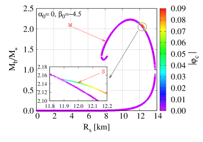
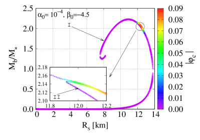
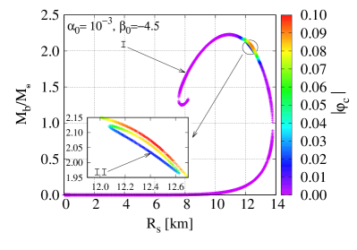
Figure 2: $M_{b}-R_{S}$ diagrams are shown for $\mu=4.8\times 10^{-13}\,\mathrm{eV}$ and $\beta_{0}=-4.5$, as well as $\alpha_{0}=0$ (top left), $\alpha_{0}=10^{-4}$ (top right) and $\alpha_{0}=10^{-3}$ (bottom panel). The color scale measures the central value of $|\varphi|$. Whereas the S and W branches connect at two points when $\alpha_{0}=0$, the S branch splits in two for nonzero $\alpha_{0}$ with each part connecting to GR-like models in such a way that we obtain a “loop” of models separate from the main branch of solutions. We refer to the main branch as branch I and to the loop as branch $II$.

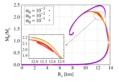
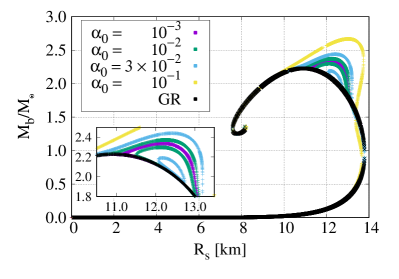
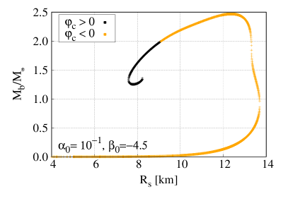
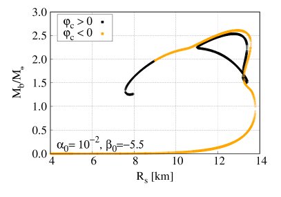
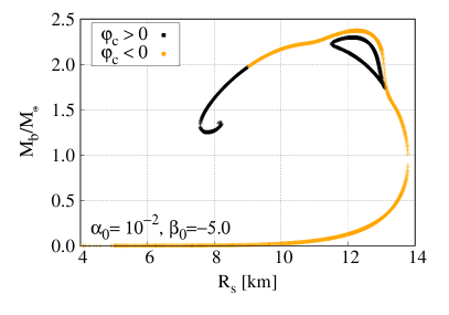
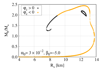
Figure 3: $M_{b}-R_{S}$ diagrams are shown for a scalar mass $\mu=4.8\times 10^{-13}$ with $\beta_{0}=-4.5$ (left) and $-5$ (right). As we increase $\alpha_{0}$, the loop of branch $II$ solutions shrinks in size and eventually disappears. For reference, we include the GR branch in the right panel.

Figure 4: Distribution of scalarized NS models based on the sign of $\varphi_{c}$ in the $M_{b}-R_{S}$ plane for $\mu=4.8\times 10^{-13}\,\mathrm{eV}$ and, from top-left to bottom-right, $(\alpha_{0},\beta_{0})=(10^{-1},-4.5)$, $(10^{-2},-5.5)$,    $(10^{-2},-5)$, $(3\times 10^{-2},-5)$. The orange points represent models with $\varphi_{c}<0$ whereas the black ones have $\varphi_{c}>0$. The type $II$ models on the loop differ in the sign of $\varphi_{c}$ from the nearby main branch $I$ models. Furthermore, we always observe a sign flip at the high-density end of branch $I$ (around $R_{S}\approx 8\,\mathrm{km}$ in the figure) but these NS models are unstable; cf. Sec. 4.5.

When $\alpha_{0}=0$, our system of equations (13)-(17) is invariant under the transformation $\varphi\to-\varphi$. In this case, each strongly scalarized model consists of two solutions that only differ by a minus sign in the scalar-field profile. Additionally to this degenerate scalarized branch, there exists a branch with zero scalar field, i.e. the set of models we also obtain in GR.

A nonzero $\alpha_{0}$ breaks the degeneracy of the strongly scalarized branch which now splits into two branches with unequal macroscopic properties and whose scalar field magnitudes differ at a level $\mathcal{O}(\alpha_{0})$. This split is illustrated in Fig. 2 where we consider NS models in the $M_{b}-R_{S}$ plane for $\mu=4.8\times 10^{-13}\,\mathrm{eV}$, $\beta_{0}=-4.5$ and different value of $\alpha_{0}$. For $\alpha_{0}=0$, we see that the scalarized branch directly connects to the GR branch. For $\alpha_{0}\neq 0$, we obtain a weakly scalarized branch W with $\varphi=\mathcal{O}(\alpha_{0})$ in place of the GR models. In terms of their mass $M_{b}$ and radius $R_{S}$, however, these models are barely distinguishable from their GR counterparts, and we refer to them as “GR like” models. The strongly scalarized branch S, on the other hand, splits into two, each of them connecting to separate parts of the GR-like branch in such a way that we obtain one loop of models that is separated from the single, large branch; cf. the insets in the top right and bottom panels of Fig. 2. We find the gap between the loop and the main branch to be proportional to $\alpha_{0}$ and independent of $\beta_{0}$. For small but nonzero $\alpha_{0}$, we thus find two sets of solutions: A branch $I$ that approximately follows the $M_{b}-R_{S}$ curve of GR for small and for large central density $\rho_{c}$, and a separate branch $II$ on a closed loop located in the region where strong scalarization occurs. The central baryon density strictly increases as we move along branch $I$, starting at $(M_{b},R_{S})=(0,0)$. We note that branches $I$ and $II$ both contain weakly as well as strongly scalarized models. Instead, their distinction arises from the separation of the loop from the main branch of models.

As we increase $\alpha_{0}$, however, the loop of branch $II$ solutions shrinks and eventually disappears, leaving branch $I$ as the only class of solutions. This remaining branch approximately overlaps with the GR family in the very high and low $\rho_{c}$ regime but shows a strong bulge of strongly scalarized solutions when $\rho_{c}$ has values comparable to nuclear density. In agreement with the literature, we observe that these scalarized models can reach significantly larger masses and radii than their GR counterparts. We illustrate these features in Fig. 4 for $\beta_{0}=-4.5$ and $-5$, but note that this behaviour occurs universally in all cases we have studied.

We conclude the discussion of the $\alpha_{0}$ dependence with a subtle observation we make throughout our computations: For all NS models of branch $II$ the central scalar field value has the same sign; $\varphi_{c}>0$ for our convention. For the vast majority (though not all) branch $I$ solutions, $\varphi_{c}$ has the opposite sign; $\varphi_{c}<0$ in our case. We display this observation graphically in Fig. 4 for several combinations of $\beta_{0}$ and $\alpha_{0}$. We note, however, that branch $I$ always contains a swap in $\mathrm{sign}(\varphi_{c})$ at very large central baryon density: we always observe $\varphi_{c}>0$ as $\rho_{c}\rightarrow\infty$.

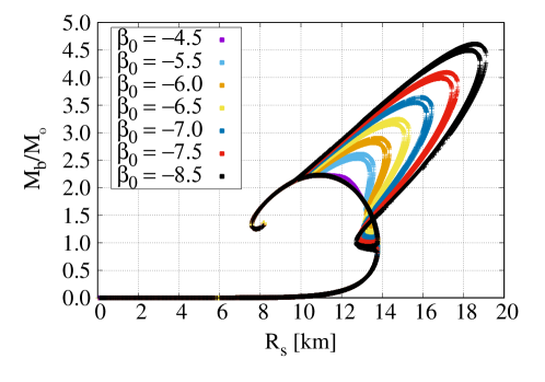
Figure 5: $M_{b}-R_{S}$ diagrams are shown for several values of $\beta_{0}$ in the regime of spontaneous scalarization $\beta_{0}<-4.35$. The other scalar field parameters are $\mu=-4.8\times 10^{-13}$ eV, $\alpha_{0}=10^{-2}$. For increasingly negative values of $\beta_{0}$, the S branch extends to larger values of the NS radius and baryon mass.

4.4 Dependence on $\beta_{0}$

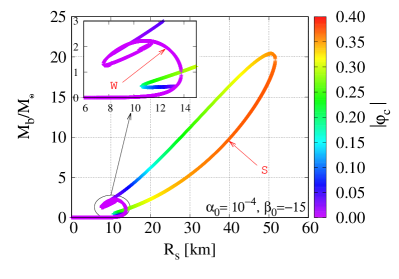
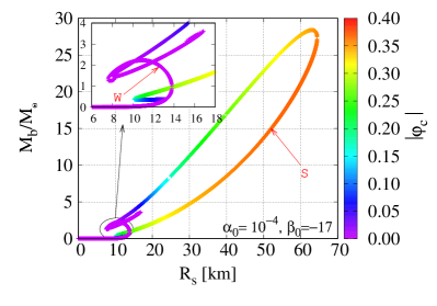
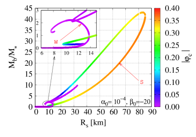
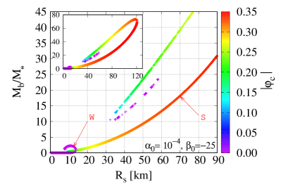
Figure 6: $M_{b}-R_{S}$ diagrams are shown for $\mu=4.8\times 10^{-13}\,\mathrm{eV}$ and $\alpha_{0}=10^{-4}$, as well as $\beta_{0}=-15$ (top left), $\beta_{0}=-17$ (top right), $\beta_{0}=-20$ (bottom left) and $\beta_{0}=-25$ (bottom right panel). The color scale measures the central value of $|\varphi|$. This sequence of plots (from top left to bottom right) shows the upper end of the S branch disconnecting and separating from the W branch as $\beta_{0}$ becomes more negative.

Spontaneous scalarization is a non-linear phenomenon and driven by the quadratic coupling parameter when $\beta_{0}\lesssim-4.35$. It has already been remarked in Ramazanoğlu and Pretorius (2016), that this threshold value for strong scalarization is barely affected by the introduction of a non-zero scalar mass. Our results confirm this observation as is illustrated by the W and S branches of solutions shown in the left panel of Fig. 1 for $\beta_{0}=-4.5$, $-5$ and $-6$ with fixed $\alpha_{0}=10^{-4}$ and $\mu=4.8\times 10^{-13}\,\mathrm{eV}$. Note that the transition from weak to strong scalarization along a sequence of NS models, while strictly speaking continuous, is sufficiently abrupt to allow for a clear distinction between models belonging to branch W or S.

The three branches displayed in the left panel of Fig. 1 for $\beta_{0}=-4.5$, $-5$ and $-6$ also demonstrate the increasing deviation in terms of mass and radius of branch S models from their GR-like counterparts. Increasingly negative values of $\beta_{0}$ allow for larger maximum mass and radius; cf. also Sec. IV A in Ramazanoğlu and Pretorius (2016). This rather strong effect may provide opportunities for constraining $\beta_{0}$ through mass and radius measurement of NSs, although a reevaluation of the measurements in the framework of ST gravity (rather than assuming GR) will be required for this purpose. In Fig. 1, the strongly scalarized branch S models appear as an arc splitting off from the GR-like branch W. We always find branch S to have this qualitative shape and the size of the arc grows monotonically as $\beta_{0}$ takes on increasingly negative values. This is illustrated in Fig. 5, which displays branches W and S for several values of $\beta_{0}\leq-4.5$. This figure also demonstrates that branch S has a shape resembling an inverted ’S’; it initially splits off from branch W towards smaller radii (around $R_{S}\approx 13.5\,\mathrm{km}$ and $M_{b}\approx 1\,M_{\odot}$ in the figure) before turning around and crossing branch W towards larger $R_{S}$. Note also that for each choice of $\beta_{0}$, branch S consists of two nearby but distinct curves; this splitting results from the relatively large value $\alpha_{0}=10^{-2}$ as we have already seen in the last section; cf. the bottom right panel in Fig. 4.

For highly negative $\beta_{0}$, we obtain NS models with yet larger radius and baryon mass as illustrated in Fig. 6, where we plot branches W and S for $\beta_{0}=-15$, $-17$, $-20$, $-25$ and fixed $\alpha=10^{-4}$, $\mu=4.8\times 10^{-13}\,\mathrm{eV}$. In this figure, we also notice a new effect: the upper (in the sense of larger $\rho_{c}$) end of branch S exhibits a more complex structure. Instead of connecting to branch W, branch S appears to remain separate and curl around; cf. the insets for $\beta_{0}=-15$ and $\beta_{0}=-17$. This behaviour becomes clearer for yet more negative $\beta_{0}$: between $\beta_{0}=-20$ and $\beta_{0}=-25$, the intersection of branch S with branch W is lost and instead, branch S forms its own tail of NS models with very small central values of the scalarfield $|\varphi_{c}|$; note the magenta color of this end of branch S. Contrary to what one might guess, the NS models on this tail of branch S are still strongly scalarized; the profile $\varphi(r)$ merely reaches its maximum away from the center $r=0$.

We explore this behaviour in more detail by comparing in Fig. 7 the sequence of models obtained for $\beta_{0}=-6$ with that for $\beta_{0}=-17$, keeping $\alpha_{0}=10^{-4}$ and $\mu=4.8\times 10^{-13}\,\mathrm{eV}$ fixed. The bottom panels show the respective families in the $M_{b}-R_{S}$ diagram analogous to Fig. 6. Along the branches, we have marked several NSs by colored circles, and for these models we plot the baryon-density and scalar-field profiles $\rho(r)$, $\varphi(r)$ in the upper panels. For $\beta_{0}=-6$, we observe a simple pattern: At the lower branch point, we obtain a weakly scalarized model (“1”) with comparatively small central baryon density. As we continue along branch S, the scalar field increases in strength, reaching a maximum at maximal radius (model “3”). Beyond that point, the central baryon density $\rho_{c}$ keeps increasing, but the scalar profile weakens. Eventually (model “6”), a weakly scalarized but highly compact NS marks the smooth reconnection with branch W; note that this weakly scalarized model is located on the unstable branch of the GR-like models.

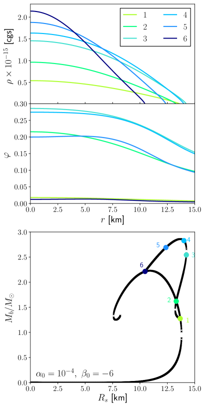
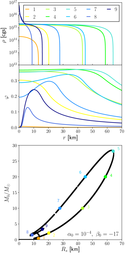
Figure 7: The branches of NS models are shown in the $M_{b}-R_{S}$ plane in the bottom panels for $\mu=4.8\times 10^{-13}\,\mathrm{eV}$, $\alpha_{0}=10^{-4}$ as well as $\beta_{0}=-6$ (left) and $\beta_{0}=-17$ (right). Several NS models are marked along the branches as colored circles. The top panels show the radial profiles of the baryon density $\rho(r)$ and the scalar field $\varphi(r)$ for these NSs using their respective color. The density profile always reaches a maximum at the origin; however, the scalar field profile in some cases reaches a peak at a non-zero radius.

The analogous results for $\beta_{0}=-17$ in the right column of Fig. 7 display a qualitatively similar behaviour near the lower branch point (model “1”); the central baryon-density and scalar-field values increase as we move along branch S (model “2”). Eventually, however, the scalar field profile changes its qualitative behaviour and peaks away from $r=0$ while the central value $\varphi_{c}$ decreases. In consequence, the upper tail of branch S now consists of models with $\varphi_{c}\approx 0$ but strong scalarization at $r>0$ and does not directly connect to branch W; compare model “8” for $\beta_{0}=-17$ with model “6” for $\beta_{0}=-6$. As branch S curls around, the scalar profile strengthens once again and we encounter models with a steep density cusp (model “9”). We cannot rigorously rule out that after further curling around, branch S might eventually connect with branch W, but our numerical results do not show any signs of this happening. We finally note the remarkable structure of these upper tail stars: A highly compact star of baryonic matter is surrounded by a shell of scalar-field (i.e. bosonic) matter. This structure is reminiscent of the atom like shape noticed for stars in massless ST gravity in Brito et al. (2016) and scalarized black holes in modified gravity  Baumann et al. (2019).

4.5 Stability of models

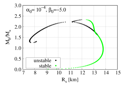
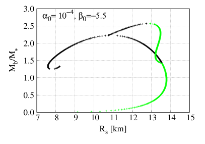
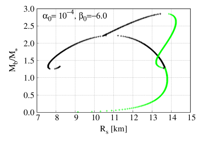
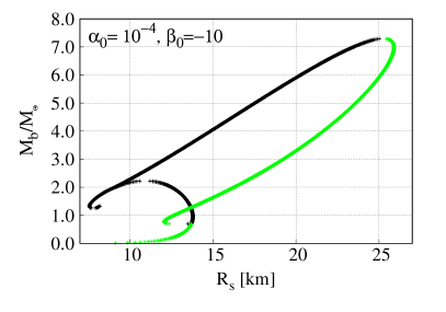
Figure 8: Plots showing the distribution of stable (green) and unstable (black) NS configurations in the $M_{b}-R_{S}$ plane. When two solutions with the same baryon mass $M_{b}$ exist, the one with the lower ADM mass is energetically favored. The scalar parameters are $\mu=4.8\times 10^{-13}$ eV, $\alpha_{0}=-10^{-4}$ and, from top left to bottom right, $\beta_{0}=-5$, $-5.5$, $-6$ and $-10$.

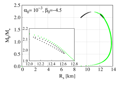
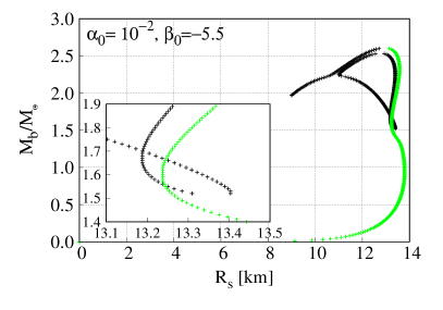
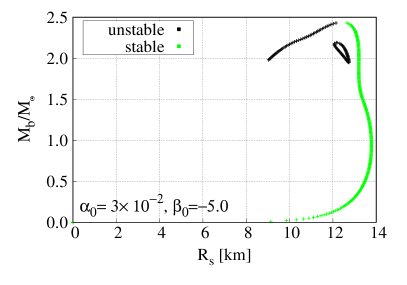
Figure 9: Same as Fig. 8 using scalar mass $\mu=4.8\times 10^{-13}$ eV, and coupling parameters from top-left to bottom, $(\alpha_{0},\beta_{0})=(10^{-3},-4.5)$, $(10^{-2},-5.5)$, $(3\times 10^{-2},-5)$.

In the previous sections, we have seen many cases where for fixed ST parameters $\alpha_{0}$, $\beta_{0}$, $\mu$ several equilibrium NS models with equal baryon mass exist; see e.g. $M_{b}=2\,M_{\odot}$ in the left panel of Fig. 1. We can analyze the stability of these models by comparing their binding energy. The model with the lowest ADM mass, i.e. strongest binding energy, represents the stable configuration and other models with equal baryon mass are expected to migrate to this configuration under perturbations. We note, however, that the physical relevance of this instability depends on the instability timescale as compared to other dynamical timescales under consideration.

Using this method, we classify in Fig. 8 stable and unstable NS models for several values of $\beta_{0}$ at fixed $\alpha=10^{-4}$ and $\mu=4.8\times 10^{-13}\,\mathrm{eV}$. The results confirm the theoretical prediction that the weakly scalarized branch W becomes unstable when strongly scalarized counterparts with equal baryon mass exist Novak (1998). Note also that the scalarized branch S exhibits a stability structure analogous to the well known GR case: The maximum mass model separates stable from unstable stars and the stable models are those with larger radius.

In Fig. 9, we analyze how the stable and unstable models spread among our “loop” branches $I$ and $II$ of Sec. 4.3 for different values of $\alpha_{0}$. The stable NSs are the strongly scalarized models with the largest radius, whereas the NSs on branch $II$ (i.e. on the closed loop) are always unstable. As a general pattern in all our computations, we find the models with the strongest central scalar field value $|\varphi_{c}|$ to be the stable configurations. For our convention, these always turn out to be models with $\varphi_{c}<0$; for example compare Fig. 9 with Fig. 4.

5 Conclusions

In this study, we have numerically computed solutions of spherically symmetric NSs in massive ST theory using a numerical scheme that enables us to eliminate the exponentially growing modes from the scalar field. For this purpose, we split the domain into the NS interior and the exterior from the stellar surface to infinity and discretize the resulting equations with a second-order relaxation scheme. This method enables us to compute NS spacetimes extending all the way to infinity where we can prescribe the boundary conditions in simple Dirichlet form. This formalism also provides a trivially simple implementation of the matching conditions without the need to perform interpolation.

We have used the resulting code to compute solutions of static, spherically symmetric NSs in massive ST theory and explored in detail the structure of the resulting branches of solutions in the (baryon) mass-radius plane for combinations of the linear and quadratic coupling parameters $\alpha_{0}$, $\beta_{0}$ of the ST theory and the scalar mass $\mu$. We summarize the main findings of our analysis as follows.

• In agreement with previous literature studies of NS equilibrium models in massive and massless ST gravity, we find larger values of $\alpha_{0}$ and $\beta_{0}$ to result in larger deviations from the NS solutions in GR, whereas larger values of the scalar mass tend to reduce these deviations; cf. Figs. 1 and 4.

• For $\alpha_{0}=0$, the NS models of GR are also solutions of the field equations of massive ST gravity. For $\beta\lesssim-4.35$, we find, additionally to the GR branch, the spontaneously scalarized class of NS solutions that Damour & Esposito-Farèse discovered in their original exploration of massless ST theory Damour and Esposito-Farese (1993) and that were also identified in massive ST theory in Ramazanoğlu and Pretorius (2016). These solutions are invariant under the scalar field transformation $\varphi\rightarrow-\varphi$.

• A non-zero $\alpha_{0}$ breaks this degeneracy and results in a dissection of the branches around the branch points; instead of the two connected branches of scalarized and non-scalarized solutions for $\alpha_{0}=0$, we now find a main branch $I$ and a smaller loop of branch $II$ solutions; cf. Fig. 2. The solutions on branches $I$ and $II$ are characterized by different signs of the central scalar-field value $\varphi_{c}$; cf. Fig. 4.

• For sufficiently negative $\beta_{0}$, roughly $\beta_{0}\lesssim-15$, we observe a qualitative change in the strongly scalarized branch S of solutions. Instead of smoothly approaching the weakly scalarized branch W as happens for milder $\beta_{0}$, its upper (in the sense of increasing central baryon density) tail now either crosses or completely detaches from the W branch.

• For highly negative values of $\beta_{0}$, we furthermore encounter a new type of strongly scalarized solutions at this upper end of the S branch: the maximum of the scalar field is located away from the stellar center; cf. Figs. 6, 7. In its most extreme form, these solutions are composed of highly compact NS models surrounded by a scalar shell; see e.g. Brito et al. (2016); Baumann et al. (2019) for similar “gravitational atom” like configurations in other theories of gravity.

• Whenever multiple NS models with equal baryon mass exist, we find the scalarized model to be the stable configurations in the sense of minimal binding energy. Typically, though not always, this is the model with the largest radius; cf. Figs. 8, 9. We also observe that the stable configurations agree in the sign of the central scalar field value, $\varphi_{c}<0$ in our convention.

The behavior with respect to the scalar parameters seems to be universal as we have encountered the same $M_{b}-R_{S}$ profile deviations with respect to GR for all other equations of state that we have studied. We have explored in a similar manner, though less exhaustively, the cold hybrid EOS1, EOS3 and EOSa Rosca-Mead et al. (2020), APR4 Akmal et al. (1998), 2H and HB Read et al. (2009) and observe qualitatively similar behaviour.

This research was funded by the European Union’s H2020 ERC Consolidator Grant “Matter and strong-field gravity: new frontiers in Einstein’s theory” Grant No. MaGRaTh–646597 and the STFC Consolidator Grant No. ST/P000673/1, the GWverse COST Action Grant No. CA16104, “Black holes, gravitational waves and fundamental physics”. D.G. is supported by Leverhulme Trust Grant No. RPG-2019-350, M.A. is supported by the Kavli Foundation, Computational work was performed on the SDSC Comet and TACC Stampede2 clusters through NSF-XSEDE Grant No. PHY-090003; the Cambridge CSD3 system through STFC capital Grants No. ST/P002307/1 and No. ST/R002452/1, and STFC operations Grant No. ST/R00689X/1; the University of Birmingham BlueBEAR cluster; the Athena cluster at HPC Midlands+ funded by EPSRC Grant No. EP/P020232/1; and the Maryland Advanced Research Computing Center (MARCC).