Electrostatic pair-interaction of nearby metal or metal-coated colloids at fluid interfaces

Abstract

In this paper, we theoretically study the electrostatic interaction between a pair of identical colloids with constant surface potentials sitting in close vicinity of each other at a fluid interface. By employing a simplified yet reasonable model system, the problem is solved within the framework of classical density functional theory and linearized as well as nonlinear Poisson-Boltzmann (PB) theory. Apart from providing a sound theoretical framework generally applicable to any such problem, our novel findings, all of which contradict common beliefs, include the following: first, quantitative as well as qualitative differences between the interactions obtained within the linear and the nonlinear PB theories; second, the importance of the electrostatic interaction between the omnipresent three-phase contact lines in interfacial systems; and third, the occurrence of an attractive electrostatic interaction between a pair of identical metal colloids. The unusual attraction we report on largely stems from an attractive line interaction which although scales linearly with the size of the particle, can compete with the surface interactions and can be strong enough to alter the nature of the total electrostatic interaction. Our results should find applications in metal or metal-coated particle-stabilized emulsions where densely packed particle arrays are not only frequently observed but are sometimes required.

I Introduction

Since its discovery in the early twentieth century by Ramsden Ram03 and Pickering Pic07 , stabilizing emulsions using colloidal particles instead of surfactants has become a standard technique. This new class of emulsions are popularly known as Pickering emulsions and finds application in diverse areas such as food Ray14 ; Ber15 ; Pic15 , cosmetic Ray14 ; Tan15 ; Mar16-1 , petroleum Uma18 , pharmaceutical or biomedical Son12 ; Lin13 ; Son13 ; He13 , and optical industries Ede16 , among others. Major advantages that make Pickering emulsions in general preferable over conventional surfactant-stabilized emulsions are its enhanced stability and reduced toxicity Wu16 ; Mar20 . Another important aspect is the availability of a wide range of particles differing in their composition and shape Bin17 ; Yan17 ; Gho19 . Among them, metal colloids are gaining increasing attention owing to their numerous applications facilitated by the advancement of opto-electronics and nanotechnology in the twenty-first century Sca18 .

Self-assembly of metal particles at fluid interfaces together with distinct optical, electrical, and catalytic properties of metal particles are exploited in liquid like mirrors Yoc03 ; Fan13 , sensors Sah12 ; Ede13 ; Pag14 , detectors Cec13 , filters Smi14 , antennas Ede13 , controllable and targeted drug delivery equipment Son12 ; Lin13 ; Son13 ; He13 , plasmonic rulers Tur12 , or in purification processes Cro10 . Due to their antimicrobial effect, silver particle stabilized emulsions are suitable for biomedical and textile applications Sam17 . For many of these applications, particularly for optical applications, a regular array of particles is needed which can be easily achieved at fluid interfaces. Contrary to the topological defects commonly observed for solid-liquid interfaces, the fluidic nature of these interfaces allows them to self-heal without any external influence, leading to strikingly uniform films spanning over large areas Cie10 ; Smi16 . Moreover, due to their defect-free nature such structures are easy to reproduce and being fluidic, they are easily deformable Smi16 .

Even a nanoparticle, while at fluid interfaces, typically feels a strong trapping potential several orders of magnitude larger than the thermal energy, originating from the reduction of the fluid-fluid interfacial area Bin00 ; Bin06 ; Boo15 . This restricts the motion of the particle to be only along the interfacial plane. Consequently, the arrangement of particles within a monolayer and the stability of the overall structure are largely dictated by their lateral interaction. For charged particles, one of the dominant contributions to the total lateral interaction usually comes from the electrostatic origin Oet08 ; Luo12 ; Kra16 ; Isa17 , which is the focus of the present study.

If the inter-particle separations are large, then, from the electrostatic point of view, the system behaves like a set of interacting point dipoles as the counter-ion cloud surrounding each particle differs in the two adjacent fluid media and leads to an effective dipole normal to the interfacial plane Pie80 . The large separation distance also allows for a point-particle assumption and for an analytical solution using the linearized PB theory or the Debye-Hückel (DH) theory Hur85 . Whereas this simple yet useful picture has sparked the interest of a bunch of subsequent studies Kra16 ; Ave02 ; Nik02 ; Wue04 ; Fry07 ; Dom08 ; Mas10 ; Gao15 ; Pet16 ; Rah19 , little is known about the opposite limit, i.e., when the inter-particle separation is small compared to the size of the particles. Clearly, the dipolar assumption fails in this situation.

Most of the few recent efforts Maj14 ; Maj16 ; Lia16 ; Maj18-1 ; Maj18-2 targeted toward addressing the short inter-particle separations have considered particles with constant surface charge densities, which, at a simplistic level, describes dielectric or insulating particles the best Der16 ; Mar16-2 . Conductive metal particles, on the other hand, are characterized by constant surface potentials Mar16-2 . In a very recent publication Zig20 , the interaction between particles at an air-water interface with constant surface potentials only in the portions immersed in water is addressed using the linearized PB theory. However, equipotential metal particle surfaces carry the same constant potential irrespective of the adjacent fluid phase. Not only that, metal particle stabilized emulsions often feature significantly polarizable oils Yen14 ; Smi16 ; Sca18 which behave quite differently compared to air. Moreover, the use of the linearized PB theory at short separations may not be accurate as well Maj16 . Therefore, a proper description of the electrostatic interaction between a pair of metal particles situated very close to each other at a fluid interface is still lacking and we aim toward filling this gap here.

The short separation situation we consider is frequently encountered experimentally for metal particle-stabilized emulsions Ede16 ; Sca18 ; Pag14 ; Smi16 ; Rei04 ; Coh07 ; Yen14 ; Too16 . In fact, for nanoplasmonic mirrors or detectors, in order to get substantial signal, one needs densely packed array of relatively big particles ($\gtrsim 40\,\mathrm{nm}$ in diameter) with average surface to surface distance being smaller than the particle radii Ede16 ; Sca18 ; Cec13 ; Fla10 . Not only that, our study could be equally useful for interfacial Janus colloids Fer15 ; Sto19 ; Die20 when the metal caps face each other or for core-shell particles consisting of metal shells with metallic or cost-effective non-metallic cores Pag14 ; Abi07 . One should also note that, strictly speaking, all particles including the metal ones in electrolyte solutions are charge-regulated Maj18-3 ; San19 . We do not account for such complexities here. However, the constant potential case should still remain insightful as the charge regulation solution is bounded by constant charge and constant potential limits Mar16-2 .

In order to tackle the problem efficiently, we use some justified approximations (see Fig. 1). First, the short inter-particle separation is exploited to treat the particles as flat plates by ignoring their curvatures. This assumption, motivated by the Derjaguin approximation, has been used before in this context as well Maj14 ; Maj16 ; Maj18-1 . Second, we assume the fluid-fluid interface to be flat as interfacial deformations are usually negligible for smooth particles up to a few micrometers in size Kra00 ; Sta00 ; Oet08 ; Ana16 . Moreover, we consider a $90^{\circ}$ liquid-particle contact angle which corresponds to the maximum reduction of interfacial area for any spherical particle and has been particularly shown to be pivotal for the entrapment of nanoparticles Dua04 ; Hu12 . Several other existing theoretical models also rely on these latter two assumptions Dom08 ; Upp14 ; Nal14 ; Bos16 ; Zig20 .

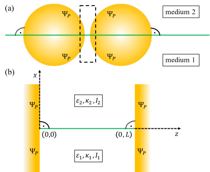
Figure 1: (a) Graphical illustration of the system under consideration. Two identical particles (represented by the yellow circles) with constant surface potentials $\Psi_{P}$ are sitting next to each other at a flat interface (indicated by the green horizontal line) formed by two immiscible electrolytes denoted as medium “1” (for $x<0$) and as medium “2” (for $x>0$). The surface-to-surface separation between the particles is small compared to their size and each particle is submerged equally in the two fluid phases corresponding to a liquid-particle contact angle of $90^{\circ}$. (b) Enlarged view of a model system that approximates the boxed region in part (a). Owing to their short separation, the particles are assumed to be parallel flat plates situated at $z=0$ and $z=L$ and aligned vertically with respect to the fluid interface. Fluid phase “1” (“2”) has dielectric constant $\varepsilon_{1}$ ($\varepsilon_{2}$). The ionic strength of the added binary monovalent salt and the corresponding inverse Debye length in medium “1” (“2”) are given by $I_{1}$ ($I_{2}$), and $\kappa_{1}$ ($\kappa_{2}$), respectively.

The electrostatic problem for the resulting model system, as depicted in Fig. 1(b), is studied within the framework of classical density functional theory (DFT) which requires the free energy of the system as the only input. A subsequent minimization of this free energy then leads to the governing equation for the electrostatic potential along with the boundary conditions and the ensuing effective interaction, which automatically ensures self-consistency, can also be attained easily. We solve the problem separately using the linearized PB theory and the nonlinear PB theory. In each case, the effective interaction is decomposed into parts proportional to the surface areas of the plates and to the lengths of the three-phase contact lines. We also provide results for the separation-independent interactions, i.e., surface, interface, and line tensions present in the system. Apart from offering a comparison, the analytically obtained results within the linear theory also serve as checks for those obtained numerically within the nonlinear PB theory in proper limits. Our results feature several novel aspects that contradict common beliefs. First, we show that the interaction of the three-phase contact lines plays a crucial role in determining the nature of the total electrostatic interaction. This is not intuitively obvious as the line part to the total electrostatic interaction scales linearly with the size of the particle whereas the surface parts scale with the square of the size of the particle. Second, our findings suggest that, depending upon the specific system under consideration, the interaction obtained within the linearized PB theory can differ quantitatively as well as qualitatively from that obtained within the nonlinear PB theory. While the quantitative differences are not unexpected at small inter-particle separations, the qualitative one is indeed surprising. Third and as a most striking result, it is shown that the electrostatic interaction of identical metal particles at fluid interface is not necessarily always repulsive. The unexpected attraction stems from the line interaction energy which can be repulsive as well as attractive and, depending upon the system, can be strong enough to alter the nature of the total electrostatic interaction.

II Model and formalism

In a Cartesian coordinate system, the region of interest is the space $x\in(-\infty,\infty)$, $z\in[0,L]$ bounded by two plates positioned at $z=0$ and $z=L$ and filled with two immiscible fluid phases creating an interface at $x=0$ (see Fig. 1(b)). As the plates mimic metal surfaces, they are equipotential. Moreover, they are considered to be identical and are modeled as constant potential surfaces, i.e., they carry the same surface potential $\Psi_{P}$ irrespective of the separation distance $L$ between them. The fluid phase occupying the space $x<0$ $(x>0)$ is denoted as medium “1” (“2”). The dissolved salt is a simple binary compound composed of oppositely charged monovalent ingredients only. Consequently, the ionic strength equals the salt concentration and its bulk value in medium $i\in\{1,2\}$ is given by $I_{i}$. The background solvents, i.e., the fluids are treated as structureless incompressible linear dielectrics with dielectric constants $\varepsilon_{i}=\varepsilon_{r,i}\varepsilon_{0}$, $i\in\{1,2\}$, where $\varepsilon_{r,i}$ is the relative permittivity of medium $i$ and $\varepsilon_{0}$ is the vacuum permittivity. Please note that the length scale of our interest is the Debye screening length $\kappa_{i}^{-1}=\sqrt{\varepsilon_{r,i}/\left(8\pi\ell_{B}I_{i}\right)}$, where $\ell_{B}=e^{2}/\left(4\pi\varepsilon_{0}k_{B}T\right)$ denotes the vacuum Bjerrum length with the elementary positive charge $e$, the Boltzmann constant $k_{B}$, and the temperature $T$. Therefore, any phenomena occurring on a smaller length scale such as the scale of bulk correlation length or molecular length are discarded. This includes the structures formed in the liquids due to the presence of the salt ions or of the surfaces and the interface, and associated changes in the ion number density profiles $n_{\pm}\left(\mathbf{r}\right)$ Bie12 . Thus, both the ionic strength profile $I(\mathbf{r})$ and the dielectric constant profile $\varepsilon(\mathbf{r})$ vary steplike at the interface. However, we consider the variation in the local charge density $e\left[n_{+}\left(\mathbf{r}\right)-n_{-}\left(\mathbf{r}\right)\right]$ as it varies on the scale of the Debye length. On this length scale, the salt ions can be considered as point like objects and, following the standard practice within a mean-field theory, we ignore any ion-ion correlation. With all these, the grand canonical density functional in the units of the thermal energy $k_{B}T=1/\beta$ for our system, which is in equilibrium with the ion reservoirs provided by the bulk of the two fluid media, is given by

$$\beta\Omega\left[n_{\pm}\right]= \int\limits_{V}d^{3}r\Bigg{[}\sum\limits_{k=\pm}n_{k}\left(\mathbf{r}\right)\left\{\ln\left(\frac{n_{k}\left(\mathbf{r}\right)}{\zeta_{k}}\right)-1+\beta V_{k}\left(\mathbf{r}\right)\right\}$$

$$+\frac{\beta\mathbf{D}\left(\mathbf{r},\left[n_{\pm}\right]\right)^{2}}{2\varepsilon\left(\mathbf{r}\right)}\Bigg{]}$$

$$+\beta\Psi_{P}\int\limits_{\partial V}d^{2}r\hat{\text{\boldmath$\nu$}}\left(\mathbf{r}\right)\cdot\mathbf{D}\left(\mathbf{r},\left[n_{\pm}\right]\right).$$ (1)

In this expression, within the curly brackets, the first two terms correspond to the entropic ideal gas contribution of the ions with fugacities $\zeta_{\pm}$, the third term describes the contribution due to ion solvation expressed via an external potential $V_{\pm}\left(\mathbf{r}\right)$ acting on the ions. The term quadratic in the electric displacement vector $\mathbf{D}$ includes all the Coulomb electrostatic interactions in the system due to the presence of surface charges and ions, whereas the last term stands for the work done by the system to maintain the plates at a constant surfaces potential $\Psi_{P}$. The integration volume $V$ is the space $(x,z)\in(-\infty,\infty)\times[0,L]$ enclosed by the bounding surfaces $\partial V$, i.e., the two plates at $z=0$ and $L$ with $\hat{\text{\boldmath$\nu$}}\left(\mathbf{r}\right)$ denoting the unit outward normal to these surfaces. Although Eq. (1) is central to both the linearized and the nonlinear PB theory and what we do next is in principle the same within both the theories, the ways in which we proceed from here differ slightly as the former is analytically tackleable whereas one needs to resort to numerical techniques for the latter. Hence, below we discuss them separately.

II.1 Linear theory

Within the linearized PB theory, one assumes that the deviations in the ion number densities compared to their bulk values are small. Consequently, $\Omega\left[n_{\pm}\right]$ is expanded in terms of these small deviations to obtain $\widetilde{\Omega}\left[n_{\pm}\right]$ by retaining terms up to quadratic order in the expansion. A minimization of $\widetilde{\Omega}\left[n_{\pm}\right]$ with respect to $n_{\pm}$ then provides the equilibrium profiles $n^{\text{eq}}_{\pm}$ which, together with the Gauss’s law, leads to the linearized PB or DH equation

$$\Delta\Psi_{i}\left(\mathbf{r}\right)=\kappa_{i}^{2}\left[\Psi_{i}\left(\mathbf{r}\right)-\Psi_{b,i}\right]$$ (2)

to be solved for the electrostatic potential $\Psi_{i}\left(\mathbf{r}\right)$ in medium $i\in\left\{1,2\right\}$ (see Chapter 2 of Beb18 for details). In conjunction with this, the following boundary conditions, which also come out of the minimization process, must be satisfied. First, both the electrostatic potential and the $x$-component of the electric displacement vector should be continuous at the fluid-fluid interface, i.e., at any given $z$-value, $\Psi\left(x=0^{-},z\right)=\Psi\left(x=0^{+},z\right)$, and $\varepsilon_{1}\partial_{x}\Psi_{1}\left(x=0^{-},z\right)=\varepsilon_{2}\partial_{x}\Psi_{2}\left(x=0^{+},z\right)$ should hold true. Second, the electrostatic potential must match the surface potential of the two plates at $z=0$ and $L$: $\Psi_{i}\left(x,z=0\right)=\Psi_{i}\left(x,z=L\right)=\Psi_{P}$, irrespective of the value of $x$. Moreover, the electrostatic potential needs to be finite while approaching $x\rightarrow\pm\infty$ which, in fact, is a prerequisite for using a Derjaguin-like approximation and is typically satisfied due to electrostatic screening. $\Psi_{b,i}$ in Eq. (2) refers to the bulk electrostatic potential in medium $i\in\left\{1,2\right\}$. By construction, the bulk electrostatic potential profile $\Psi_{b}(\mathbf{r})$ reads as

$$\Psi_{b}(\mathbf{r})=\begin{cases}\Psi_{b,1}=0&(\text{in medium ``1''})\\ \Psi_{b,2}=\Psi_{D}&(\text{in medium ``2''}).\end{cases}$$

This difference ($\Psi_{D}$) arises from contrasting solvation energies of the ions in the two media and is known as the Donnan potential or Galvani potential difference Bag06 .

As shown in Sec. III.1, Eq. (2) is analytically solvable for our set-up. Once the electrostatic potentials $\Psi_{i}\left(\mathbf{r}\right)$ are known, they are used to calculate $n_{\pm}^{\text{eq}}[\Psi]$ by considering the ion density profiles as functionals of $\Psi$. Finally, inserting these $n_{\pm}^{\text{eq}}[\Psi]$ back into the expression for $\widetilde{\Omega}\left[n_{\pm}\right]$, one obtains the grand potential $\widetilde{\Omega}\left(L\right)=\widetilde{\Omega}\left[n_{\pm}\left[\Psi\right]\right]$ of our system which combines the following contributions distinctly different from each other according to their origin:

$$\widetilde{\Omega}\left(L\right)= \sum\limits_{i\in\left\{1,2\right\}}\left[\Omega_{b,i}V_{i}+\left(\gamma_{i}+\omega_{\gamma,i}\left(L\right)\right)A_{i}\right]$$

$$+\gamma_{1,2}A_{1,2}+\left(\tau+\omega_{\tau}\left(L\right)\right)\ell.$$ (3)

Here, $\Omega_{b,i}=-2I_{i}/\beta$ is the osmotic or entropic energy contribution due to the ideal gas formed by the ions expressed per volume $V_{i}$ of medium $i\in\{1,2\}$, $\gamma_{i}$ is the surface tension acting between each plate and medium $i$, $\omega_{\gamma,i}(L)$ is the surfaces interaction energy density between the portions of the plates immersed in and acting through medium $i$, $A_{i}$ is the total surface area of the two plates immersed in medium $i$, $\gamma_{1,2}$ is the interfacial tension between medium “$1$” and medium “$2$”, $A_{1,2}$ is the total area of the fluid-fluid interface; $\tau$ is the line tension present at the three-phase contact lines at $(0,0)$ and $(0,L)$, and $\omega_{\tau}(L)$ is the contribution due to interaction between the contact lines expressed per total length $\ell$ of the two contact lines. Clearly, $\gamma_{i}$ and $\tau$ are $L$-independent as they result from the interaction of a single plate with its adjacent fluid(s). For the purpose of calculating the effective interaction between two colloids as shown in Fig. 1(a), the terms involving $\Omega_{b,i}$ and $\gamma_{1,2}$ in Eq. (3) also become irrelevant as the total volume of the fluids and the total area of the fluid-fluid interface, which not only include the boxed region in Fig. 1(a) but also the outer space, do not change while changing the separation distance $L$ between the colloids. Therefore, the effective inter-particle interaction, which is what we are interested in, is exclusively dictated by the contributions involving the surface interaction energy density $\omega_{\gamma,i}(L)$ and the line interaction energy density $\omega_{\tau}(L)$. Please note that they are constructed such that $\omega_{\gamma,i}(L\rightarrow\infty)\rightarrow 0$ and $\omega_{\tau}(L\rightarrow\infty)\rightarrow 0$.

II.2 Nonlinear theory

Within the nonlinear PB theory, the density functional in Eq. (1) is directly minimized with respect to $n_{\pm}$ which provides the equilibrium profiles $n_{\pm}^{\text{eq}}$ for the ion number densities. Using these profiles, one finally ends up getting the nonlinear PB equation

$$\Delta\left(\beta e\Psi_{i}\left(\mathbf{r}\right)\right)=\kappa_{i}^{2}\sinh\left[\beta e\left(\Psi_{i}\left(\mathbf{r}\right)-\Psi_{b,i}\right)\right]$$ (4)

along with the same boundary conditions as listed below Eq. (2) to be satisfied by the electrostatic potential $\Psi_{i}\left(\mathbf{r}\right)$ in medium $i\in\left\{1,2\right\}$. In principle, after solving Eq. (4), the grand potential $\Omega\left(L\right)$ can also be obtained from Eq. (1) by inserting the equilibrium ions profiles $n_{\pm}^{\text{eq}}\left[\Psi\right]$. However, in order to facilitate the whole process, we use the density functional

$$\beta\Omega_{\text{fem}}\left[\Psi\right]= \int\limits_{V}d^{3}r\Bigg{[}2I(\mathbf{r})\cosh\left\{\beta e\left(\Psi(\mathbf{r})-\Psi_{b}(\mathbf{r})\right)\right\}$$

$$+\frac{\beta\varepsilon(\mathbf{r})}{2}\left\{\left(\partial_{x}\Psi(\mathbf{r})\right)^{2}+\left(\partial_{z}\Psi(\mathbf{r})\right)^{2}\right\}\Bigg{]}$$ (5)

instead and obtain the electrostatic potential $\Psi\left(\mathbf{r}\right)$ (defined as $\Psi\left(\mathbf{r}\right)=\Psi_{1}\left(\mathbf{r}\right)$ for $x<0$ and $\Psi\left(\mathbf{r}\right)=\Psi_{2}\left(\mathbf{r}\right)$ for $x>0$) by minimizing it numerically using Rayleigh-Ritz-like finite element method Bra10 . Please note that the minimization of this functional with respect to $\Psi\left(\mathbf{r}\right)$ also results in the PB equation [Eq. (4)] together with all the boundary conditions that need to be satisfied. Once the potential $\Psi\left(\mathbf{r}\right)$, which minimizes Eq. (5) is obtained, it can be inserted back in Eq. (5) to obtain $\Omega_{\text{fem}}^{\text{min}}\left(L\right)$ which, at equilibrium, is related to the grand potential $\Omega\left(L\right)$ by $\Omega\left(L\right)=-\Omega_{\text{fem}}^{\text{min}}\left(L\right)$. Without loss of generality, we first rewrite Eq. (5) by expanding the function $\cosh\left\{\beta e\left(\Psi(\mathbf{r})-\Psi_{b}(\mathbf{r})\right)\right\}$ in a Taylor series,

$$\beta\Omega_{\text{fem}}^{(m)}\left[\Psi\right]= \int\limits_{V}d^{3}r\Bigg{[}2I(\mathbf{r})\sum\limits_{k=0}^{m}\frac{\left\{\beta e\left(\Psi(\mathbf{r})-\Psi_{b}(\mathbf{r})\right)\right\}^{2k}}{\left(2k\right)!}$$

$$+\frac{\beta\varepsilon(\mathbf{r})}{2}\left\{\left(\partial_{x}\Psi(\mathbf{r})\right)^{2}+\left(\partial_{z}\Psi(\mathbf{r})\right)^{2}\right\}\Bigg{]},$$ (6)

where $m$ can be interpreted as the degree of nonlinearity. For $m=1$, one recovers the linearized PB problem whereas $m\rightarrow\infty$ corresponds to the full nonlinear problem. We increase $m$ in Eq. (6) step by step starting from $m=1$. For each $m$-value, $\Omega^{(m)}\left(L\right)=-\Omega_{\text{fem}}^{(m)\text{min}}\left(L\right)$ is calculated and further decomposed into different interaction parameters as described in Eq. (3),

$$\Omega^{(m)}\left(L\right)=-\Omega_{\text{fem}}^{(m)\text{min}}\left(L\right)= \sum\limits_{i\in\left\{1,2\right\}}\left[\Omega_{b,i}V_{i}+\left(\gamma_{i}+\omega_{\gamma,i}\left(L\right)\right)A_{i}\right]$$

$$+\gamma_{1,2}A_{1,2}+\left(\tau+\omega_{\tau}\left(L\right)\right)\ell,$$ (7)

with all the quantities in the right hand side carrying the same meaning as defined for Eq. (3). Numerical extraction of these contributions requires solving some subproblems with the following set-ups: (i) single fluid medium “1” (“2”) spanning the lower (upper) half-space in Fig. 1(b) in the absence of any plates; the corresponding grand potential density $\Omega_{b,i}=-2I_{i}/\beta$ is easily obtained by simply setting $\Psi(\mathbf{r})=\Psi_{b}(\mathbf{r})$ and $\Psi_{P}=0$ in Eq. (6), (ii) only the two fluid media present in the absence of any plates, (iii) a single plate present in contact with a single semi-infinite fluid medium, (iv) two plates interacting across a single fluid medium, and (v) a single plate touching two semi-infinite fluids in its one side. A sequential subtraction of the grand potentials obtained for these subproblems then enables one to separate all the contributions in Eq. (7). For $m=1$, the resulting interaction parameters are checked against those obtained analytically within the linear theory. With increasing $m$, for all the different system parameters considered here, we observe that $\Omega^{(m)}\left(L\right)=-\Omega_{\text{fem}}^{(m)\text{min}}\left(L\right)$ saturates for $m\geq 4$. Therefore, in what follows, we call the results for $m=4$ as the solutions under the nonlinear theory. This is in accordance with the conclusion of Ref. Maj16 and is not unexpected since we deal with the potentials of similar order of magnitude in both studies.

III Results and discussion

III.1 Linear theory

III.1.1 Electrostatic potential

Our goal is to find the electrostatic potential which satisfies the DH equation (Eq. (2)) and the associated boundary conditions as mentioned below Eq. (2) for the system depicted in Fig. 1(b). To achieve this, we first dissect the original problem into the following subproblems: (i) two plates with constant surface potentials $\Psi_{P}$ interacting across fluid “1” or fluid “2” with bulk potential $\Psi_{b,1}$ or $\Psi_{b,2}$, respectively; the resulting potential in both cases depend on $z$-coordinate only, (ii) two fluids phases occupying the two half spaces $(x\gtrless 0)$ forming an interface at $x=0$ in the absence of any plates; the corresponding electrostatic potential, which is solely $x$-dependent, and the electric displacement vector are continuous at the interface. Exploiting the linear nature of the governing equation, i.e., the DH equation, if we simply add the solution for medium $i$ in subproblem (i) with the corresponding ones obtained in subproblem (ii), the sums are also solutions of the DH equation and they satisfy most of the boundary conditions except for the continuity of the total electrostatic potentials at the interface. In order to get rid of this inconsistency we then seek for a correction function which also satisfies the DH equation and which, when added to the previously obtained sums, meets the remaining continuity condition without affecting any of the conditions that are already fulfilled. Such a function can easily be constructed by means of Fourier series expansion (for details, please see Chapter 3 of Ref. Beb18 ). With all these, the final expressions for the electrostatic potentials in medium $i\in\{1,2\}$ read as

$$\Psi_{i}(x,z\,;L)= \Psi_{b,i}+\left(\Psi_{P}-\Psi_{b,i}\right)\frac{\sinh\left(\kappa_{i}z\right)-\sinh\left(\kappa_{i}\left(z-L\right)\right)}{\sinh\left(\kappa_{i}L\right)}$$

$$-\sum\limits_{j\in\left\{1,2\right\}}^{j\neq i}\sum\limits_{n=1,3,\dots}^{\infty}\left(-1\right)^{i}4n\pi\varepsilon_{j}p_{n,j}(L)\xi_{n}(L)$$

$$\times e^{-p_{n,i}(L)|x|}\sin\left(\frac{n\pi z}{L}\right),$$ (8)

where

$$\xi_{n}(L)=\frac{\frac{\Psi_{D}}{n^{2}\pi^{2}}-\frac{\Psi_{P}}{n^{2}\pi^{2}+\kappa_{1}^{2}L^{2}}+\frac{\left(\Psi_{P}-\Psi_{D}\right)}{n^{2}\pi^{2}+\kappa_{2}^{2}L^{2}}}{\varepsilon_{1}p_{n,1}(L)+\varepsilon_{2}p_{n,2}(L)}$$

and $p_{n,i}(L)=\sqrt{\frac{n^{2}\pi^{2}}{L^{2}}+\kappa_{i}^{2}}$. The first two terms in Eq. (8) together is the solution of the subproblem (i), i.e., potential distribution for two plates with constant potentials $\Psi_{P}$ interacting across medium $i$. The remainder represents the correction function. The solution of the subproblem (ii) is canceled by the first term ($n=0$) of the series representing the correction function. From Eq. (8), one can trivially check that $\Psi_{i}(z=0)=\Psi_{i}(z=L)=\Psi_{P}$. In the limit $x\rightarrow\pm\infty$, the series term vanishes because of the exponential function and one is left with the first two terms describing the potential due to two plates with constant surface potential $\Psi_{P}$ interacting across medium $i$ with bulk potential $\Psi_{b,i}$. This is exactly the situation far away from the interface. Upon approaching simultaneously the limits $x\rightarrow\pm\infty$ and $L\rightarrow\infty$, the series term vanishes and the second term reduces to an exponentially varying function characteristic of a single plate placed in contact with an electrolyte solution. In addition, if we set $z\rightarrow\infty$ in Eq. (8), we recover the bulk potential $\Psi_{b,i}$. As a side remark, we note that in the limit $L\rightarrow\infty$ only, the second term reduces to an exponentially decaying potential and the sum can be converted to an integral over $q=n\pi/L$. The resulting expression corresponds to the potential due to a single plate with surface potential $\Psi_{P}$ placed in contact with two immiscible fluids spanning the regions $x\gtrless 0$ with $z>0$. This can also be derived independently with the help of Fourier transforms (for details, please refer to the derivation of Eqs. (3.115) and (3.116) in Ref. Beb18 ).

III.1.2 Interaction energies

With the electrostatic potential at hand, we can use it to calculate the grand potential $\widetilde{\Omega}\left(L\right)=\widetilde{\Omega}\left[n_{\pm}\left[\Psi\right]\right]$ and to derive the expressions for the interaction parameters of our system. As defined in Eq. (3), this is achieved by distinguishing the terms proportional to $V_{i}$, $A_{i}$, $A_{1,2}$, and $\ell$. Moreover, the $L$-independent interactions are recognized in the terms proportional to $A_{i}$ and $\ell$ by taking the limit $L\rightarrow\infty$ (for details, please see Chapter 4 of Ref. Beb18 ).

The surface tensions, as defined in Eq. (3), acting between each surface and its adjacent fluid medium $i\in\{1,2\}$ is given by

$$\gamma_{i}=-\frac{\varepsilon_{i}\kappa_{i}}{2}\left(\Psi_{P}-\Psi_{b,i}\right)^{2},$$ (9)

and the surface interaction energy between two surfaces with total area $A_{i}$ in medium $i\in\{1,2\}$ is given by

$$\omega_{\gamma,i}(L)=\frac{\varepsilon_{i}\kappa_{i}\left(\Psi_{P}-\Psi_{b,i}\right)^{2}}{2}\left[1+\frac{1-\cosh\left(\kappa_{i}L\right)}{\sinh\left(\kappa_{i}L\right)}\right].$$ (10)

Whereas the amplitudes of both $\gamma_{i}$ and $\omega_{\gamma,i}(L)$ depend on $\varepsilon_{i}$, $\kappa_{i}$, $\Psi_{P}$, and $\Psi_{b,i}$, the decay rate of $\omega_{\gamma,i}(L)$ is uniquely governed by $\kappa_{i}$. In the limit of vanishing separation between the plates, Eq. (10) predicts a finite, repulsive interaction: $\omega_{\gamma,i}(L\rightarrow 0)=\frac{\varepsilon_{i}\kappa_{i}}{2}\left(\Psi_{P}-\Psi_{b,i}\right)^{2}$. Contrary to a constant charge boundary condition, this non-divergent behavior in the $L\rightarrow 0$ limit is characteristic of a constant potential boundary condition Mar16-2 . In the large asymptotic limit, Eq. (10) provides $\omega_{\gamma,i}(L\rightarrow\infty)\simeq\varepsilon_{i}\kappa_{i}\left(\Psi_{P}-\Psi_{b,i}\right)^{2}\left[e^{-\kappa_{i}L}-\frac{e^{-2\kappa_{i}L}}{2}\right]$. Therefore, as dictated by the leading order term, the surface interaction $\omega_{\gamma,i}(L)$ decays monotonically $\sim e^{-\kappa_{i}L}$ for large separations between the plates.

The interfacial tension per total interfacial area $A_{1,2}$ acting between the two fluid media reads as

$$\gamma_{1,2}=-\frac{\varepsilon_{1}\varepsilon_{2}\kappa_{1}\kappa_{2}\Psi_{D}^{2}}{2\left(\varepsilon_{1}\kappa_{1}+\varepsilon_{2}\kappa_{2}\right)}.$$ (11)

As expected, the interfacial tension depends only on the properties of the two fluid media and not on any plate properties. Consequently, the expression for $\gamma_{1,2}$ does not differ from what one obtains for plates with constant surface charge densities Maj18-1 .

The line tension acting at both the three-phase contact lines expressed per total length of the two contact lines is given by

$$\tau= -\frac{\varepsilon_{1}\varepsilon_{2}\left(\Psi_{P}-\Psi_{D}\right)}{\pi}\int\limits_{0}^{\infty}dq\frac{p_{1}(q)}{p_{2}(q)}q^{2}\xi(q)+\frac{\varepsilon_{1}\varepsilon_{2}\Psi_{P}}{\pi}\int\limits_{0}^{\infty}dq\frac{p_{2}(q)}{p_{1}(q)}q^{2}\xi(q)$$

$$-\frac{\varepsilon_{1}\varepsilon_{2}\Psi_{D}}{\pi}\int\limits_{0}^{\infty}\frac{dq}{\varepsilon_{1}p_{1}(q)+\varepsilon_{2}p_{2}(q)}\left[\frac{\left(\kappa_{2}^{2}-\kappa_{1}^{2}\right)\Psi_{D}}{p_{1}(q)p_{2}(q)+\frac{\kappa_{1}}{\kappa_{2}}p_{2}(q)^{2}}\right.\left.-\frac{\left(\kappa_{2}^{2}-\kappa_{1}^{2}\right)\Psi_{P}}{p_{1}(q)p_{2}(q)}-\frac{\kappa_{1}\kappa_{2}\Psi_{D}}{\varepsilon_{1}\kappa_{1}+\varepsilon_{2}\kappa_{2}}\left(\frac{\varepsilon_{1}}{p_{1}(q)+\kappa_{1}}+\frac{\varepsilon_{2}}{p_{2}(q)+\kappa_{2}}\right)\right],$$ (12)

with

$$\xi(q)=\frac{\frac{\Psi_{D}}{q^{2}}-\frac{\Psi_{P}}{q^{2}+\kappa_{1}^{2}}+\frac{\left(\Psi_{P}-\Psi_{D}\right)}{q^{2}+\kappa_{2}^{2}}}{\varepsilon_{1}p_{1}(q)+\varepsilon_{2}p_{2}(q)}$$

and $p_{i}(q)=\sqrt{q^{2}+\kappa_{i}^{2}}$, and the line interaction energy (defined in Eq. (3)) acting between the two three-phase contact lines is given by

$$\omega_{\tau}(L)= -2\varepsilon_{1}\varepsilon_{2}\left(\Psi_{P}-\Psi_{D}\right)\sum\limits_{n=1,3,\dots}^{\infty}\xi_{n}(L)\frac{n^{2}\pi^{2}}{L}\frac{p_{n,1}(L)}{p_{n,2}(L)}$$

$$+2\varepsilon_{1}\varepsilon_{2}\Psi_{P}\sum\limits_{n=1,3,\dots}^{\infty}\xi_{n}(L)\frac{n^{2}\pi^{2}}{L}\frac{p_{n,2}(L)}{p_{n,1}(L)}$$

$$-2\varepsilon_{1}\varepsilon_{2}\Psi_{D}\sum\limits_{n=1,3,\dots}^{\infty}\xi_{n}(L)p_{n,1}(L)p_{n,2}(L)L$$

$$+\frac{\varepsilon_{1}\varepsilon_{2}\kappa_{1}\kappa_{2}\Psi_{D}^{2}L}{4\left(\varepsilon_{1}\kappa_{1}+\varepsilon_{2}\kappa_{2}\right)}-\tau,$$ (13)

with $\xi_{n}(L)$ and $p_{n,i}(L)$ as defined below Eq. (8) and the expression for $\tau$ given in Eq. (12). In the limit of vanishing separation ($L\rightarrow 0$) between the plates, all the terms in Eq. (13) vanish except for the last term, i.e., $\tau$. Therefore, in this limit $\omega_{\tau}(L)$ stays finite unlike what one observes for constant charge boundary condition Maj14 ; Maj18-1 . Using the relation $\sum\limits_{n=1,3,\dots}^{\infty}\frac{1}{n^{2}}=\frac{\pi}{8}$ it is trivial to see that the terms $\propto L$, i.e., the third and the fourth terms in Eq. (13) cancel each other in the large asymptotic limit ($L\rightarrow\infty$). The rest of the terms together lead to an overall exponential decay of the line interaction $\omega_{\tau}(L)$ in this limit. A striking observation regarding the line interaction for constant surface charge density boundary condition is that it is independent of the Donnan potential $\Psi_{D}$ Maj14 ; Maj18-1 . On the contrary, as Eq. (13) suggests, $\omega_{\tau}(L)$ does depend on $\Psi_{D}$ while using a constant surface potential boundary condition. This is indeed reasonable since the line part essentially captures the effects of the interface to the total inter-plate interaction and the contrast in the bulk potential should get reflected in it.

III.2 Nonlinear theory

In this subsection, we discuss the results within the nonlinear theory and compare them with those obtained using the linear theory in Sec. III.1. In order to present our numerically obtained results and to gain insight into the variations of different parameters efficiently, we use dimensionless quantities. Accordingly, $\omega_{\gamma,i}(L)$ and $\omega_{\tau}(L)$ are expressed as $\beta\omega_{\gamma,i}(L)/\kappa_{1}^{2}$ and $\beta\omega_{\tau}(L)/\kappa_{1}$, respectively and their behavior is studied as functions of the scaled separation $\kappa_{1}L$. In doing so, the number of dimensionless free parameters reduces to only four: $\beta e\Psi_{P}$, $\beta e\Psi_{D}$, $I=I_{2}/I_{1}$, and $\varepsilon=\varepsilon_{2}/\varepsilon_{1}$. As the permittivities of oils used in typical experimental systems widely vary Yen14 ; Smi16 ; Sca18 , we consider two experimental systems differing significantly in their fluid contents for our discussion. The variations of different system parameters with respect to one of these systems are also presented which allow one to infer what could be expected to happen for an arbitrary general system.

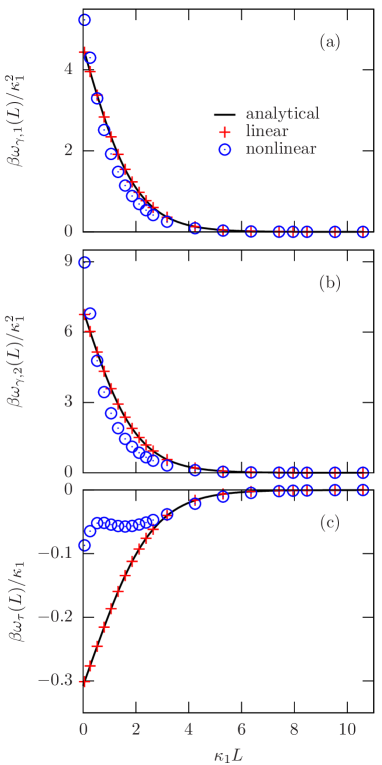
Figure 2: (a) - (b) Variations of the surface interaction energy densities $\omega_{\gamma,1}(L)$ and $\omega_{\gamma,2}(L)$, both expressed in units of $\kappa_{1}^{2}/\beta$ and (c) variation of the line interaction energy density $\omega_{\tau}(L)$ expressed in units of $\kappa_{1}/\beta$ as functions of the scaled separation $\kappa_{1}L$ between the two surfaces for standard set of parameters ($\beta e\Psi_{P}=-3$, $\beta e\Psi_{D}=1$, $\varepsilon=62/72$, and $I=0.85$) corresponding to particles trapped at a water–lutidine interface. As shown by all the plots, the numerically obtained results for $m=1$ in Eq. (7) match perfectly with the analytically obtained results within the linearized PB theory. Whereas both $\omega_{\gamma,1}(L)$ and $\omega_{\gamma,2}(L)$ are repulsive and decay monotonically with increasing separation distance $\kappa_{1}L$ under linearized as well as nonlinear PB theory, the linear theory underestimates them at very short separations and overestimates at larger separations. On the other hand, the linear theory fails to qualitatively predict the correct variation for $\omega_{\tau}(L)$. Whereas $\omega_{\tau}(L)$ is attractive everywhere in the linear case, it can be attractive as well as repulsive within the nonlinear theory.

III.2.1 Water–lutidine system

As our first example, we take a system with particles at a water–lutidine (2,6-dimethylpyridine) interface at temperature $T=313\,\mathrm{K}$ above the critical temperature Gra93 . The water-rich phase is denoted as the medium “1” and the lutidine-rich phase as the medium “2”. The dissolved salt is NaI with bulk ionic concentrations $I_{1}=1\,\mathrm{mM}$ and $I_{2}=0.85\,\mathrm{mM}$ which leads to a Donnan potential estimated to be $1\,k_{B}T/e$ Ine94 ; Bie12 . The relative permittivities of the two fluids are $\varepsilon_{r,1}=72$ and $\varepsilon_{r,2}=62$ Ram57 ; Lid02 . Typically metal surfaces are negatively charged in an electrolyte solution Smi17 . Therefore, the particles are considered to be carrying a constant potential $\Psi_{P}=-3\,k_{B}T/e\approx-77\,\mathrm{mV}$. Please note that the surface potential is expected to be slightly higher than the zeta potentials usually measured in experiments. Therefore, the dimensionless parameters of our system, which we call as the standard system, are $I=0.85$, $\varepsilon=62/72$, $\beta e\Psi_{D}=1$, and $\beta e\Psi_{P}=-3$.

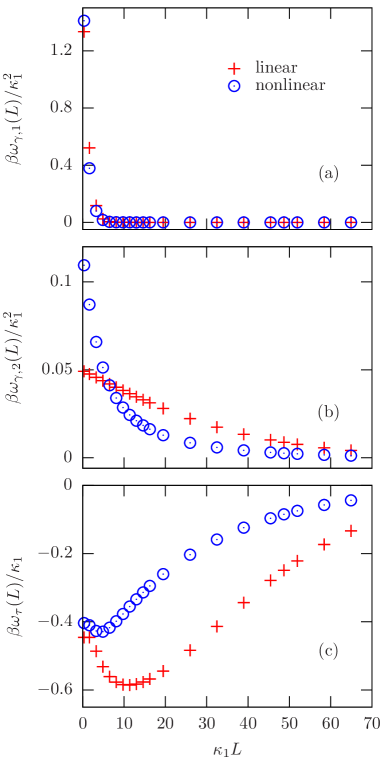
Figure 3: (a) - (b) Variations of the surface interaction energy densities $\omega_{\gamma,1}(L)$ and $\omega_{\gamma,2}(L)$, both expressed in units of $\kappa_{1}^{2}/\beta$ and (c) variation of the line interaction energy density $\omega_{\tau}(L)$ expressed in units of $\kappa_{1}/\beta$ as functions of the scaled separation $\kappa_{1}L$ between the two surfaces. The parameters ($\beta e\Psi_{P}=-3$, $\beta e\Psi_{D}=3.8$, $\varepsilon=10.3/80$, and $I=2.9\times 10^{-4}$) used for the plots correspond to a system consisting of particles trapped at a water–octanol interface. As shown by all the plots, whereas both $\omega_{\gamma,1}(L)$ and $\omega_{\gamma,2}(L)$ are repulsive and decay monotonically with increasing separation distance $\kappa_{1}L$ under linearized as well as nonlinear PB theory, the linear theory underestimates them at very short separations and overestimates at larger separations. Regarding the variation of the line interaction $\omega_{\tau}(L)$, whereas the linear theory qualitatively predicts the correct behavior, it is inaccurate in predicting the magnitude of $\omega_{\tau}(L)$ and the location of the minimum.

The ensuing interaction energies between the two plates are presented in Fig. 2. For all the plots, the data points correspond to the numerically obtained results and the solid lines represent the analytically obtained expressions in Subsection III.1.2. Figure 2(a) shows the variation of the scaled surface interaction energy density $\omega_{\gamma,1}(L)$ acting between the portions of the plates in contact with medium “1” as function of the varying scaled separation $L$. As one can see, both the linear and the nonlinear theory predict a monotonically decaying repulsive interaction between the plates, and as expected, the numerically obtained results corresponding to $m=1$ in Eq. (7) match perfectly with the analytically obtained solution within the linear theory throughout the range of separations considered here. While the results within the two theories qualitatively agree with each other, the linear theory underestimates the interaction at very short separations and overestimates at relatively larger separations. This discrepancy gradually drops down as the separation distance is increased. Similar conclusions can be drawn from Fig. 2(b) concerning the variation of the scaled surface interaction energy density $\omega_{\gamma,2}(L)$ acting between the portions of the plates in contact with medium “2” as function of the varying scaled separation $L$ within the two theories. The magnitudes of $\omega_{\gamma,1}(L)$ and $\omega_{\gamma,2}(L)$ are of the same order as the two fluids do not significantly differ in their properties and the surface potentials of the plates are also the same in both media. However, the surface interaction in medium “2” is slightly stronger compared to medium “1” due to less screening. Figure 2(c) shows the variation of the scaled line interaction energy $\omega_{\tau}(L)$ as function of the scaled separation $L$ within both the theories. As one can infer, within the range of separations considered, the linear theory predicts a monotonically decaying attractive interaction with increasing separation distance between the plates. However, within the nonlinear theory the line interaction shows a qualitatively different behavior. It changes non-monotonically upon increasing the separation distance, shows a maximum at $\kappa_{1}L\approx 1$ followed by a minimum at around $\kappa_{1}L\approx 2$ and then decays monotonically. Clearly, the interaction is repulsive in between the maximum and the minimum. Please note that both the maximum and the minimum occur at distances much larger than the molecular length scale (typically a few angstroms). Not only that, up to around $\kappa_{1}L\approx 2$, the linear theory significantly overestimates the strength of the line interaction as well.

III.2.2 Water–octanol system

Water–lutidine falls in a class of systems where the bulk properties, i.e., the relative permittivities and the bulk ionic strengths, and consequently the Debye screening lengths vary little in the two fluid phases. Although such combination of immiscible fluids are used in experiments Smi17 ; Sca18 , there is another frequently used category of systems where moderately polarizable oils are used Sca18 . Therefore, as a second example, we consider a system consisting of particles trapped at a water–octanol interface. At room temperature $T=300\,\mathrm{K}$ these two fluids are characterized by significantly different relative permittivities with $\varepsilon_{r,1}=80$ (for water as medium “1”) and $\varepsilon_{r,2}=10.3$ (for octanol as medium “2”). The ion-partitioning at this interface results in highly contrasting bulk ionic strengths as well. For $I_{1}=10\,\mathrm{mM}$ in the water phase, $I_{2}=2.9\times 10^{-3}\,\mathrm{mM}$ in the octanol phase, leading to a Donnan potential $\Psi_{D}\approx 3.8\,k_{B}T/e$. The associated inverse Debye lengths in the two phases are given by $\kappa_{1}\approx 0.324\,\mathrm{nm^{-1}}$ and $\kappa_{2}\approx 0.015\,\mathrm{nm^{-1}}$. The particles are considered to be carrying the same surface potentials as before, i.e., $\Psi_{P}=-3\,k_{B}T/e\approx-77\,\mathrm{mV}$. Hence, the dimensionless parameters of this system are given by $I=2.9\times 10^{-4}$, $\varepsilon=10.3/80$, $\beta e\Psi_{D}=3.8$, and $\beta e\Psi_{P}=-3$.

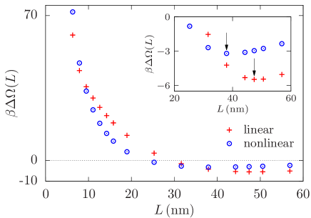
Figure 4: Variation of total interaction energy $\Delta\Omega(L)=\omega_{\gamma,1}(L)A_{1}+\omega_{\gamma,2}(L)A_{2}+\omega_{\tau}(L)\ell$ between the two surfaces expressed in the units of $1/\beta$ as a function of the separation $L$ for a water–octanol system charecterised by $\beta e\Psi_{P}=-3$, $\beta e\Psi_{D}=3.8$, $\varepsilon=10.3/80$, $I_{2}=2.9\times 10^{-2}\,\mathrm{mM}$, $I_{1}=0.1\,\mathrm{M}$, $A_{2}=A_{1}=2573\,\mathrm{nm}^{2}$, and $\ell=114\,\mathrm{nm}$. The total effective surface areas $A_{i}$ and the total effective length of the three-phase contact lines are rough estimates for $60\,\mathrm{nm}$ particles. As one can see, the interaction energy decreases initially, shows a minimum, and finally increases monotonically within both the linear (red crosses) and the nonlinear PB theories (blue open circles). The initial decreases in the interaction energy corresponds to a positive effective force at short separations $L$, implying that the interaction is repulsive there. Beyond the position of the minimum, it turns into an attractive one. Whereas this feature remains the same within the two theories, the location of the minimum (as indicated by the arrows in the inset) shifts from $L\approx 48\,\mathrm{nm}$ to a significantly shorter separation $L\approx 38\,\mathrm{nm}$ while calculated using the nonlinear PB theory. Therefore, the particles will come much closer than what is predicted by the linear theory.

The resulting interactions for this system are shown in Fig. 3. Both $\omega_{\gamma,1}(L)$ and $\omega_{\gamma,2}(L)$, as shown in Figs. 3(a) and 3(b), respectively predict monotonically decaying repulsive interactions under the linear as well as the nonlinear theory. But, as before, the linear theory underestimates the interactions at very short separations whereas overestimates them at relatively larger separations. Depending upon the fluid medium and the separation distance $L$, this mismatch can be significant (see, for example, the data presented in Fig. 3(b)). Except for very short separations, the interaction in medium “2”, i.e., $\omega_{\gamma,2}(L)$ is stronger compared to that in medium “1” (presented by $\omega_{\gamma,1}(L)$). This is due to a weaker screening in the medium “2” compared with medium “1” which is evident from the rapid decay of $\omega_{\gamma,1}(L)$ in Fig. 3(a). At very short separations, however, one enters into the electric double layer and with decreasing separations, the ions, which are strongly attracted to the surfaces, need to be removed. As the ionic strength is higher in medium “1”, the system needs to remove more ions leading to a stronger repulsion compared to medium “2”. Concerning the line interaction energy $\omega_{\tau}(L)$, as shown in Fig. 3(c), it decays non-monotonically with increasing separation $L$ between the two plates. Initially its magnitude increases implying a repulsive interaction, which, after the occurrence of a minimum, turns into an attractive interaction. Although the linear theory predicts the qualitative behavior correctly, it significantly overestimates the strength of the interaction over the entire range of separations considered here and also fails to accurately locate the position of the minimum. It is worth mentioning that the line interaction for water–octanol system is much stronger compared to that for the water–lutidine system owing to greater contrast between the combination of the fluids used. While comparing the magnitudes in Figs. 2 and 3, please note that $\kappa_{1}\approx 0.324\,\mathrm{nm^{-1}}$ for the water–octanol system whereas $\kappa_{1}\approx 0.106\,\mathrm{nm^{-1}}$ for the water–lutidine system.

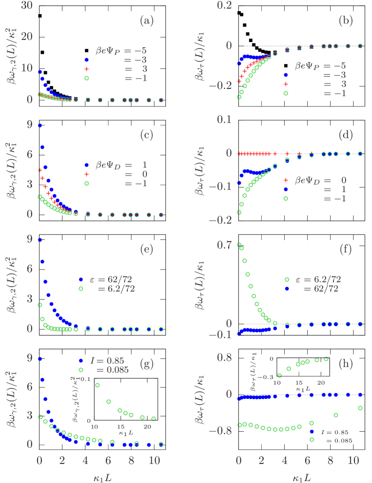
Figure 5: Variations of the surface interaction energy density $\omega_{\gamma,2}(L)$ expressed in units of $\kappa_{1}^{2}/\beta$ (left panels) and variations of the line interaction energy density $\omega_{\tau}(L)$ expressed in units of $\kappa_{1}/\beta$ (right panels) as functions of the scaled separation $\kappa_{1}L$ between the two plates for various sets of free dimensionless parameters $\beta e\Psi_{P}$ (panels (a) and (b)), $\beta e\Psi_{D}$ (panels (c) and (d)), $\varepsilon$ (panels (e) and (f)), and $I$ (panels (g) and (h)). In all cases, only a single parameter has been changed at a time from the standard water–lutidine system and the interactions are compared. The parameters that are changed are mentioned in each plot. As shown by all the plots in the left panel, $\omega_{\gamma,2}(L)$ is always repulsive and it increases with increasing difference $\beta e\left|\Psi_{P}-\Psi_{D}\right|$ or $\beta e\Psi_{D}$ or $\varepsilon$. On the other hand, whereas an increase in $I$ strengthens $\omega_{\gamma,2}(L)$ at very short separations, it weakens $\omega_{\gamma,2}(L)$ at relatively larger separations. As shown by panel (b), $\omega_{\tau}(L)$ shows a maximum followed by a minimum for strongly or moderately negative surface potentials. On the other hand, for positively charged or weakly negatively charged particles $\omega_{\tau}(L)$ remains attractive everywhere. With increasing values of $\beta e\Psi_{D}$, $\omega_{\tau}(L)$ changes from overall attractive to a non-monotonically varying behavior showing a maximum at very short separations followed by a minimum at larger separations. For $\beta e\Psi_{D}=0$, $\omega_{\tau}(L)$ almost vanishes as the contrast between the two fluid media reduces in this case. With decreasing $\varepsilon$, the height of the maximum of $\omega_{\tau}(L)$ increases and it shifts to the left whereas the minimum becomes shallow and shifts to larger distances. On the other hand, with decreasing $I$, whereas the position of the maximum does not change, the minimum shifts to larger distances and the magnitude of $\omega_{\tau}(L)$ increases. Insets of panels (g) and (h) show the variations at larger separation distances as the Debye screening length is larger for the smaller $I$ values.

So far we have presented results concerning all the different parts, i.e., $\omega_{\gamma,1}(L)$, $\omega_{\gamma,2}(L)$ and $\omega_{\tau}(L)$ to the total electrostatic interaction. This indeed allows one to investigate the system in a detailed way and gain better insight from a theoretical point of view. We are also not required to restrict ourself to fixed particle sizes. However, experimentally it might be challenging to disentangle all these individual interaction parameters. Also, one might reasonably wonder about the relative importance of the line interaction energy $\omega_{\tau}(L)$ in comparison with the surface interaction energies $\omega_{\gamma,1}(L)$ and $\omega_{\gamma,2}(L)$. As Eq. (3) or (7) suggests, the surface contributions to the total grand potential are proportional to the surface areas of the plates whereas the line contribution scales with the length of the three-phase contact lines. Therefore, for large surfaces, the surface contributions dominate anyway in due course. But what happens for typical system parmeters? To address these concerns, we present in Fig. 4 the total interaction energy $\Delta\Omega(L)=\omega_{\gamma,1}(L)A_{1}+\omega_{\gamma,2}(L)A_{2}+\omega_{\tau}(L)\ell$ (i.e., the total $L$-dependent part in Eq. (3) or (7)) for a water–octanol system with $\beta e\Psi_{P}=-3$, $\beta e\Psi_{D}=3.8$, $\varepsilon=10.3/80$, $I_{2}=2.9\times 10^{-2}\,\mathrm{mM}$, $I_{1}=0.1\,\mathrm{M}$, $A_{2}=A_{1}=2573\,\mathrm{nm}^{2}$, and $\ell=114\,\mathrm{nm}$. The effective areas $A_{i}$ and and effective length of the three-phase contact lines are rough estimates for $60\,\mathrm{nm}$ particles. The quantity, i.e., $\Delta\Omega(L)$ we plot in Fig. 4 is related to the effective electrostatic force $F(L)=-\partial\left(\Delta\Omega\right)/\partial L$ which can be considered as experimentally more relevant quantity. As the plot suggests, the total interaction energy $\Delta\Omega(L)$ initially decreases with increasing separation, reaches a minimum (marked with the arrows in the inset of Fig 4) and then increases within both the linear and the nonlinear PB theories. This implies a repulsive interaction till the position of the minimum and an attractive interaction beyond that. As both the surface parts are repulsive in Fig. 3 throughout the range of separations $\kappa_{1}L$ considered here, the attractions clearly come from the line parts. Although both the linear and the nonlinear theory predict an attractive interaction beyond certain separations, the equilibrium separation (given by the position of the minimum) decreases significantly from $L\approx 48\,\mathrm{nm}$ to $L\approx 38\,\mathrm{nm}$ while calculated using the nonlinear PB thoery. It is worth mentioning that the line interaction starts to be comparable in magnitude with the surface parts at much shorter distances. Therefore, depending on the system, the line contribution can indeed dominate over the surface contributions even for typical system parameters. We also note that, as discussed in Subsection III.2.3 and as can be seen in Figs. 5(a) and 5(b), the minimum can be moved to smaller separations and its depth can be increased by reducing the surface potential $\beta e\Psi_{P}$ as the magnitudes of the surface parts reduce whereas that of the line part increases with decreasing surface potential.

III.2.3 Variation of system parameters

Now we discuss the effects of changing the free parameters, i.e., $\beta e\Psi_{P}$, $\beta e\Psi_{D}$, $\varepsilon$, and $I$, of our system within the nonlinear PB theory. The comparisons are done with respect to the standard (water–lutidine) system. Please note that, the permittivity ratio $\varepsilon=\varepsilon_{2}/\varepsilon_{1}$ and the ionic concentration ratio $I=I_{2}/I_{1}$ can vary due to changes in the respective quantities in either or both fluids. However, the resulting total interaction is sensitive only to the ratios $\varepsilon$ and $I$. For our analysis, we have chosen to vary $\varepsilon$ and $I$ by changing $\varepsilon_{2}$ and $I_{2}$, respectively while keeping $\varepsilon_{1}$ and $I_{1}$ fixed. Therefore, only the surface interaction $\omega_{\gamma,2}(L)$ in medium “2” and $\omega_{\tau}(L)$ changes due to such variations but $\omega_{\gamma,1}(L)$ remains unaltered. $\omega_{\gamma,1}(L)$ is also independent of the Donnan potential $\beta e\Psi_{D}$. However, it changes due to variation in $\beta e\Psi_{P}$ but this happens in a fashion similar to what one observes for $\omega_{\gamma,2}(L)$. Therefore, here we show only the variations of $\omega_{\gamma,2}(L)$ and $\omega_{\tau}(L)$ upon changing the system parameters.

As one can see from Fig. 5(a), the surface interaction $\omega_{\gamma,2}(L)$ in medium “2” increases with absolute value of the increasing contrast between surface potential $\Psi_{P}$ and the bulk potential $\Psi_{b,2}$. Consequently, no change is observed while varying $\beta e\Psi_{P}$ from $3$ to $-1$ (please note that $\beta e\Psi_{b,2}=1$ here). Similarly, $\omega_{\gamma,2}(L)$ increases with increasing Donnan potential $\beta e\Psi_{D}$ and the permittivity ratio $\varepsilon$; see Figs. 5(c) and 5(e). Concerning the variation of $\omega_{\gamma,2}(L)$ upon increasing the ionic strength ratio $I$, $\omega_{\gamma,2}(L)$ increases at very short separations whereas it decreases at relatively larger separations; see Fig. 5(g). At these larger separations, with increasing ionic concentration, electrostatic screening increases. Therefore, the effective electrostatic interaction diminishes. However, at very short separations, within the electric double layer, the number of ions strongly attracted to the surfaces is more for higher ionic strengths. Consequently, more work needs to be done in order to decrease the separation distance as it requires removing these ions. This results in higher values for $\omega_{\gamma,2}(L)$. Please note that irrespective of the specific values of the system parameters $\omega_{\gamma,2}(L)$ is always repulsive.

The variations of $\omega_{\tau}(L)$ with different system parameters are shown in the right panel of Fig. 5. As one can see from Fig. 5(b), $\omega_{\tau}(L)$ shows a maximum followed by a minimum for strongly or moderately negative surface potentials. Therefore, the line interaction can be repulsive as well as attractive depending upon the separation distance $L$. On the other hand, for positively charged or weakly negatively charged particles the line interaction $\omega_{\tau}(L)$ remains attractive everywhere and decays monotonically. With increasing values of $\beta e\Psi_{D}$, $\omega_{\tau}(L)$ changes from overall attractive monotonically decreasing behavior to a non-monotonically varying behavior showing a maximum at very short separations followed by a minimum at larger separations; see Fig. 5(d). A special situation is presented by $\beta e\Psi_{D}=0$ which leads to an almost vanishing $\omega_{\tau}(L)$ as the contrast between the two fluid media reduces in this case. With decreasing $\varepsilon$, the height of the maximum of $\omega_{\tau}(L)$ increases and it shifts to the left whereas the minimum becomes shallow and shifts to larger distances; see Fig. 5(f). On the other hand, with decreasing $I$, whereas the position of the maximum does not change, the minimum shifts to larger distances and the magnitude of $\omega_{\tau}(L)$ increases; see Fig. 5(h).

Table 1: Values of the surface tensions $\gamma_{1}$ (third column) and $\gamma_{2}$ (fourth column) resulting from interactions of the plates across medium “1” and medium “2”, respectively, the interfacial tension $\gamma_{1,2}$ (fifth column) acting between the two fluids, and the line tension $\tau$ (last column) acting at the three-phase contact lines for all the systems considered in this study (listed in the first column). The first block represents the results for our standard water–lutidine system and the last block provides results corresponding to the water–octanol system. The intermediate blocks provide results for system where a single parameter has been changed at a time from the standard system. These systems are denoted by the parameter that is changed. The surface and the interfacial tension values are given in the units of $k_{B}T/\mathrm{nm}^{2}$ while the line tension values are provided in the units of $k_{B}T/\mathrm{nm}$. For each system, the results obtained analytically within linearized PB theory and numerically within nonlinear as well as linear PB theory are presented. As expected, the numerically obtained values for $m=1$ in Eq. (7) (denoted as ‘Linear’) agree with those obtained analytically. As it is evident from the presented values, $\gamma_{1}$, $\gamma_{2}$, and $\gamma_{1,2}$ are always negative for the systems considered here and the linear theory always underestimates their absolute values. However, the line tension $\tau$ appears to be the most sensitive to the variations in the system parameters and to the type of theory used to calculate its value. It can be positive as well as negative, decrease as well as increase and even change sign while calculating within the linear and the nonlinear theories.

		$\gamma_{1}\,(k_{B}T/\mathrm{nm}^{2})$	$\gamma_{2}\,(k_{B}T/\mathrm{nm}^{2})$	$\gamma_{1,2}\,(k_{B}T/\mathrm{nm}^{2})$	$\tau\,(k_{B}T/\mathrm{nm})$
Water–lutidine	Analytical	$-0.05116\phantom{0}$	$-0.07780\phantom{0}$	$-0.002621$	$\phantom{-}0.03255\phantom{0000}$
(Standard)	Linear	$-0.05116\phantom{0}$	$-0.07781\phantom{0}$	$-0.002621$	$\phantom{-}0.03255\phantom{0000}$
	Nonlinear	$-0.06150\phantom{0}$	$-0.1073\phantom{00}$	$-0.002635$	$\phantom{-}0.009874\phantom{000}$
$\beta e\Psi_{P}=-5$	Analytical	$-0.1421\phantom{00}$	$-0.1751\phantom{00}$	$-0.002621$	$\phantom{-}0.03309\phantom{0000}$
	Linear	$-0.1421\phantom{00}$	$-0.1751\phantom{00}$	$-0.002621$	$\phantom{-}0.03309\phantom{0000}$
	Nonlinear	$-0.2320\phantom{00}$	$-0.3464\phantom{00}$	$-0.002635$	$-0.01676\phantom{0000}$
$\beta e\Psi_{P}=-1$	Analytical	$-0.005684$	$-0.01945\phantom{0}$	$-0.002621$	$\phantom{-}0.03200\phantom{0000}$
	Linear	$-0.005685$	$-0.01945\phantom{0}$	$-0.002621$	$\phantom{-}0.03201\phantom{0000}$
	Nonlinear	$-0.005804$	$-0.02113\phantom{0}$	$-0.002635$	$\phantom{-}0.02747\phantom{0000}$
$\beta e\Psi_{P}=3$	Analytical	$-0.05116\phantom{0}$	$-0.01945\phantom{0}$	$-0.002621$	$\phantom{-}0.03091\phantom{0000}$
	Linear	$-0.05116\phantom{0}$	$-0.01945\phantom{0}$	$-0.002621$	$\phantom{-}0.03091\phantom{0000}$
	Nonlinear	$-0.06150\phantom{0}$	$-0.02113\phantom{0}$	$-0.002635$	$\phantom{-}0.01918\phantom{0000}$
$\beta e\Psi_{D}=-1$	Analytical	$-0.05116\phantom{0}$	$-0.01945\phantom{0}$	$-0.002621$	$\phantom{-}0.03091\phantom{0000}$
	Linear	$-0.05116\phantom{0}$	$-0.01945\phantom{0}$	$-0.002621$	$\phantom{-}0.03091\phantom{0000}$
	Nonlinear	$-0.06150\phantom{0}$	$-0.02113\phantom{0}$	$-0.002635$	$\phantom{-}0.01918\phantom{0000}$
$\beta e\Psi_{D}=0$	Analytical	$-0.05116\phantom{0}$	$-0.04377\phantom{0}$	$\phantom{-}0\phantom{.000000}$	$-0.000003198$
	Linear	$-0.05116\phantom{0}$	$-0.04377\phantom{0}$	$\phantom{-}0\phantom{.000000}$	$-0.000003198$
	Nonlinear	$-0.06150\phantom{0}$	$-0.05262\phantom{0}$	$\phantom{-}0\phantom{.000000}$	$-0.000003016$
$\varepsilon=6.2/72$	Analytical	$-0.05116\phantom{0}$	$-0.02460\phantom{0}$	$-0.001210$	$-0.06384\phantom{0000}$
	Linear	$-0.05116\phantom{0}$	$-0.02463\phantom{0}$	$-0.001211$	$-0.06390\phantom{0000}$
	Nonlinear	$-0.06150\phantom{0}$	$-0.03415\phantom{0}$	$-0.001224$	$-0.07482\phantom{0000}$
$I=0.085$	Analytical	$-0.05116\phantom{0}$	$-0.02460\phantom{0}$	$-0.001210$	$\phantom{-}0.06193\phantom{0000}$
	Linear	$-0.05118\phantom{0}$	$-0.02461\phantom{0}$	$-0.001210$	$\phantom{-}0.06193\phantom{0000}$
	Nonlinear	$-0.06157\phantom{0}$	$-0.03393\phantom{0}$	$-0.001223$	$\phantom{-}0.07061\phantom{0000}$
Water–octanol	Analytical	$-0.1670\phantom{00}$	$-0.005242$	$-0.001627$	$\phantom{-}0.1478\phantom{00000}$
	Linear	$-0.1677\phantom{00}$	$-0.005220$	$-0.001634$	$\phantom{-}0.1455\phantom{00000}$
	Nonlinear	$-0.2031\phantom{00}$	$-0.01217\phantom{0}$	$-0.002165$	$\phantom{-}0.1321\phantom{00000}$

It is important to note that, the equilibrium separation between the particles is determined by the total interaction energy $\Delta\Omega(L)=\omega_{\gamma,1}(L)A_{1}+\omega_{\gamma,2}(L)A_{2}+\omega_{\tau}(L)\ell$; the curves in Fig. 5 do not directly dictate it. However, they provide important informations regarding what one should expect for a given experimental set-up. For example, the surface interactions being always repulsive, inter-particle attraction can only come from the line part. As the plots suggest, the line part can either be monotonically attractive or it can change from repulsive to attractive beyond the position of a minimum at short separations. Even if it is monotonically attractive, at very short separations (below $L\approx 20\,\mathrm{nm}$) the surface parts usually dominate. Only in the case of small $\varepsilon$ values, the surface part is strongly suppressed. However, the line part itself becomes repulsive in this case (see Fig. 5(f)). The curves plotted in Figs. 2, 3 and 5 also suggest that if a minimum exists at a non-vanishing separation, it typically occurs between $L\approx 20\,\mathrm{nm}-40\,\mathrm{nm}$ (please note that $\kappa_{1}$ for Fig. 3 is different than that in Figs. 2 and 5). Therefore, in view of these results, we conclude that overall electrostatic attraction can start to kick in at or above $L\approx 20\,\mathrm{nm}$ and the particles will arrange themselves with an inter-particle separation $L\gtrsim 20\,\mathrm{nm}$. It is worth mentioning that the relevance of the line part and the precise location of the minimum not only depend on the system parameters considered in Fig. 5 but also on the surface areas exposed to the fluids and on the length of the three-phase contact line. However, from Fig. 5, one can easily say that the magnitude of the line part can be strongly enhanced by increasing the contrast in the ionic strengths in the two media (or equivalently, decreasing the ionic strength ratio $I=I_{2}/I_{1}$). On the other hand, for a given separation, the surface parts can be suppressed by decreasing the relative permittivity value, by reducing the surface potential, or by increasing the electrostatic screening. In fact, this is also evident if one compares the two experimental systems (water–lutidine and water–octanol) discussed previously.

What remain to be discussed are the $L$-independent interactions in Eqs. (3) or (7). Their values are listed in Table 1 for all the different system parameters considered here. As one can see, in all cases the numerically obtained values for $m=1$ in Eq. (7) (denoted as ‘Linear’) agrees perfectly with the analytically obtained results (denoted as ‘Analytical’) using Eqs. (9), (11), and (12). As one can see from Table 1, the surface tension $\gamma_{1}$ acting between the plates and medium “1” is always negative. However, its absolute value is higher within the nonlinear theory compared to the linear theory. Similar observations hold true for the surface tension $\gamma_{2}$ acting between the plates and medium “2”. Both of them also increases with the absolute value of the difference between the surface potential $\beta e\Psi_{P}$ and the bulk potential $\beta e\Psi_{b,i}$. As one can infer from the fourth column, the absolute value of $\gamma_{2}$ decreases with decreasing $\beta e\Psi_{D}$, $\varepsilon$, and $I$ within both the nonlinear and the linear theories. As expected, the interfacial tension $\gamma_{1,2}$ (given in the fifth column) remains unaffected due to changes in the surface potential $\Psi_{P}$ and is insensitive to the sign of the Donnan potential $\beta e\Psi_{D}$. With decreasing $\varepsilon$ and $I$, the magnitude of $\gamma_{1,2}$ also decreases. For all the situations considered here, $\gamma_{1,2}$ is always negative except for $\beta e\Psi_{D}=0$ when it vanishes completely. The quantity that is most sensitive to changes in the system parameters is the line tension $\tau$ presented in the last column. It can be positive as well as negative. Not only that, it can decrease as well as increase and even change sign while calculating within the linear and the nonlinear theories. The values for the line tensions that we obtain are within the range $0.1\,\mathrm{pN}-1\,\mathrm{pN}$, which is in accordance with the values reported in the literature Mug02 .

We note that, although not shown here, the agreement of the results corresponding to $m=1$ in Eq. (7) with those obtained analytically within the linear theory have been checked for all the systems considered here. As another check, we also observe that with decreasing $\beta e\left|\Psi_{P}-\Psi_{b,i}\right|$ values, the difference between the results within the linear and the nonlinear theory diminishes.

IV Conclusions

To summarise, by using the classical DFT formalism, we have addressed the problem of the electrostatic interaction between a pair of identical particles with constant surface potentials sitting in close proximity of each other at a fluid-fluid interface. The particles could be either monometallic, or metal coated such as Janus particles with metallic caps facing each other or core-shell particles with metallic shells. Considering a simple yet reasonable model system, which exploits the short separation between the particles, we have solved the problem within both the linear and the nonlinear PB theory. Within the linear theory, closed-form analytical solutions are obtained for all the interaction parameters present in the system. For the nonlinear PB theory, the problem is solved numerically. While the results within the linear theory are mostly quantitatively inaccurate, they can be qualitatively reliable depending upon the system. The surface interaction energies between the two particles are always found to be repulsive and monotonically decaying. However, the line interaction energy varies non-monotonically with increasing separation between the particles and it can be attractive as well as repulsive. Not only that, contrary to common expectation, it is shown that the attractive line interaction can be strong enough to dominate over the sum of the surface parts and to dictate the nature of the overall electrostatic interaction for typical experimental systems. A comparison between two typical experimental setups illustrates that the importance of the line interaction enhances with increasing contrast in the bulk properties of the two fluids forming the interface. Therefore, special attention should be given to line interaction in the vast majority of experiments performed using liquids varying starkly in their bulk properties. We also provide results concerning the interactions such as surface, line, and interfacial tensions that do not depend on the separation distance between the particles. Finally, we note that the presented theoretical framework is based only on a simple minimization of the system free energy and can, in principle, be easily be applied to related interfacial problems dealing not necessarily with planar surfaces or interfaces. Therefore, on one hand, we expect our study to directly contribute towards improving the understanding and modeling of interfacial monolayers of colloidal particles with constant surface potentials. On the other hand, we expect it to serve as a useful reference for future theoretical investigations of related problems.

This article may be downloaded for personal use only. Any other use requires prior permission of the authors and AIP Publishing. This article appeared in the Journal of Chemical Physics and may be found at J. Chem. Phys. 153, 044903 (2020).

References

- (1) W. Ramsden, Proc. R. Soc. London 72, 156 (1903).
- (2) S. U. Pickering, J. Chem. Soc. Trans. 91, 2001 (1907).
- (3) M. Rayner, D. Marku, M. Eriksson, M. Sjöö, P. Dejmek, and M. Wahlgren, Colloids Surf. A 458, 48 (2014).
- (4) C. C. Berton-Carabin and K. Schroën, Annu. Rev. Food Sci. Technol. 6, 263 (2015).
- (5) R. Pichot, L. Duffus, I. Zafeiri, F. Spyropoulos, and I. T. Norton in Particle-Stabilized Emulsions and Colloids: Formation and Applications, edited by T. Ngai and S. A. F. Bon (RSC Soft Matter Series, The Royal Society of Chemistry, 2019).
- (6) J. Tang, P. J. Quinlan, and K. Chiu Tam, Soft Matter 11, 3512 (2015).
- (7) J. Marto, L. F. Gouveia, B. G. Chiari, A. Paiva, V. Isaac, P. Pinto, P. Simões, A. J. Almeida, H. M. Ribeiro, Ind. Crop. Prod. 80, 93 (2016).
- (8) A. A. Umar, I. B. M. Saaid, A. A. Sulaimon, R. B. M. Pilus, J. Pet. Sci. Eng. 165, 673 (2018).
- (9) J. Song, J. Zhou, and H. Duan, J. Am. Chem. Soc. 134, 13458 (2012).
- (10) J. Lin, S. Wang, P. Huang, Z. Wang, S. Chen, G. Niu, W. Li, J. He, D. Cui, G. Lu, X. Chen, and Z. Nie, ACS Nano 7, 5320 (2013).
- (11) J. Song, Z. Fang, C. Wang, J. Zhou, B. Duan, L. Pu, and H. Duan, Nanoscale 5, 5816 (2013).
- (12) J. He, P. Zhang, T. Babu, Y. Liu, J. Gong, and Z. Nie, Chem. Commun. 49, 576 (2013).
- (13) J. B. Edel, A. A. Kornyshev, A. R. Kucernak, and M. Urbakh, Chem. Soc. Rev. 45, 1581 (2016).
- (14) J. Wu and G.-H. Ma, Small 12, 4633 (2016).
- (15) A. Marefati and M. Rayner, J. Sci. Food Agric. 100, 2807 (2020).
- (16) B. P. Binks, Langmuir 33, 6947 (2017).
- (17) Y. Yang, Z. Fang, X. Chen, W. Zhang, Y. Xie, Y. Chen, Z. Liu, and W. Yuan, Front. Pharmacol. 8, 287 (2017).
- (18) S. K. Ghosh and A. Böker, Macromol. Chem. Phys. 220, 1900196 (2019).
- (19) M. D. Scanlon, E. Smirnov, T. J. Stockmann, and P. Peljo, Chem. Rev. 118, 3722 (2018).
- (20) H. Yockell-Lelièvre, E. F. Borra, A. M. Ritcey, and L. V. da Silva, Appl. Opt. 42, 1882 (2003).
- (21) P.P. Fang, S. Chen, H. Deng, M. D. Scanlon, F. Gumy, H. J. Lee, D. Momotenko, V. Amstutz, F. Corte-Salazar, C. M. Pereira, Z. Yang, and H. H. Girault, ACS Nano 7, 9241 (2013).
- (22) K. Saha, S. S. Agasti, C. Kim, X. Li, and V. M. Rotello, Chem. Rev. 112, 2739 (2012).
- (23) J. B. Edel, A. A. Kornyshev, and M. Urbakh, ACS Nano 7, 9526 (2013).
- (24) J. Paget, V. Walpole, M. B. Jorquera, J. B. Edel, M. Urbakh, A. A. Kornyshev, and A. Demetriadou, J. Phys. Chem. C 118, 23264 (2014).
- (25) M. P. Cecchini, V. A. Turek, J. Paget, A. A. Kornyshev, and J. B. Edel, Nature Mater. 12, 165 (2013).
- (26) E. Smirnov, M. D. Scanlon, D. Momotenko, H. Vrubel, M. A. Méndez, P.F. Brevet, and H. H. Girault, ACS Nano 8, 9471 (2014).
- (27) V. A. Turek, M. P. Cecchini, J. Paget, A. R. Kucernak, A. A. Kornyshev, and J. B. Edel, ACS Nano 6, 7789 (2012).
- (28) S. Crossley, J. Faria, M. Shen, and D. E. Resasco, Science 327, 68 (2010).
- (29) A. Samanta, S. Takkar, R. Kulshreshtha, B. Nandan, and R. K. Srivastava, Biomed. Phys. Eng. Express 3, 035011 (2017).
- (30) F. Ciesa and A. Plech, J. Colloid Interface Sci. 346, 1 (2010).
- (31) E. Smirnov, P. Peljo, M. D. Scanlon, F. Gumy, and H. H. Girault, Nanoscale 8, 7723 (2016).
- (32) B. P. Binks and S. O. Lumsdon, Langmuir 16, 8622 (2000).
- (33) B. P. Binks and T. S. Horozov, Colloidal Particles at Liquid Interfaces (Cambridge University Press, Cambridge, 2006).
- (34) S. G. Booth and R. A. W. Dryfe, J. Phys. Chem. C 119, 23295 (2015).
- (35) M. Oettel and S. Dietrich, Langmuir 24, 1425 (2008).
- (36) M. Luo, G. K. Olivier, and J. Frechette, Soft Matter 8, 11923 (2012).
- (37) P. A. Kralchevsky, K. D. Danov, and P. V. Petkov, Philos. Trans. R. Soc. A 374, 20150130 (2016).
- (38) L. Isa, I. Buttinoni, M. A. Fernandez-Rodriguez, and S. A. Vasudevan, Europhys. Lett. 119, 26001 (2017).
- (39) P. Pieranski, Phys. Rev. Lett. 45, 569 (1980).
- (40) A. J. Hurd, J. Phys. A 18, L1055 (1985).
- (41) R. Aveyard, B. P. Binks, J. H. Clint, P. D. I. Fletcher, T. S. Horozov, B. Neumann, V. N. Paunov, J. Annesley, S. W. Botchway, D. Nees, A. W. Parker, A. D. Ward, and A. N. Burgess, Phys. Rev. Lett. 88, 246102 (2002).
- (42) M. G. Nikolaides, A. R. Bausch, M. F. Hsu, A. D. Dinsmore, M. P. Brenner, C. Gay, and D. A. Weitz, Nature 420, 299 (2002).
- (43) L. Foret and A. Würger, Phys. Rev. Lett. 92, 058302 (2004).
- (44) D. Frydel, S. Dietrich, and M. Oettel, Phys. Rev. Lett. 99, 118302 (2007).
- (45) A. Domínguez, D. Frydel, and M. Oettel, Phys. Rev. E 77, 020401 (R) (2008).
- (46) K. Masschaele, B. J. Park, E. M. Furst, J. Fransaer, and J. Vermant, Phys. Rev. Lett. 105, 048303 (2010).
- (47) P. Gao, X. Xing, Y. Li, T. Ngai, and F. Jin, Sci. Rep. 4, 4778 (2015).
- (48) P. V. Petkov, K. D. Danov, and P. A. Kralchevsky, J. Colloid Interface Sci. 462, 223 (2016).
- (49) S. E. Rahman, N. Laal-Dehghani, and G. F. Christopher, Langmuir 35, 13116 (2019).
- (50) A. Majee, M. Bier, and S. Dietrich, J. Chem. Phys. 140, 164906 (2014).
- (51) A. Majee, M. Bier, and S. Dietrich, J. Chem. Phys. 145, 064707 (2016).
- (52) Z. Lian, J. Chem. Phys. 145, 014901 (2016).
- (53) A. Majee, T. Schmetzer, and M. Bier, Phys. Rev. E 97, 042611 (2018).
- (54) A. Majee, M. Bier, and S. Dietrich, Soft Matter 14, 9436 (2018).
- (55) I. N. Derbenev, A. V. Filippov, A. J. Stace, and E. Besley, J. Chem. Phys. 145, 084103 (2016).
- (56) T. Markovich, D. Andelman, and R. Podgornik, Europhys. Lett. 113, 26004 (2016).
- (57) A. Zigelman and O. Manor, Langmuir, 36, 4942 (2020).
- (58) Y.T. Yen, T.Y. Lu, Y.C. Lee, C.C. Yu, Y.C. Tsai, Y.C. Tseng, and H.L. Chen, ACS Appl. Mater. Interfaces 6, 4292 (2014).
- (59) F. Reincke, S. G. Hickey, W. K. Kegel, and D. Vanmaekelbergh, Angew. Chem. Int. Ed. 43, 458 (2004).
- (60) I. Cohanoschi, A. Thibert, C. Toro, S. Zou, and F. E. Hernández, Plasmonics 2, 89 (2007).
- (61) A. Toor, T. Feng, and T. P. Russell, Eur. Phys. J. E 39, 57 (2016).
- (62) M. E. Flatté, A. A. Kornyshev, and M. Urbakh, J. Phys. Chem. C 114, 1735 (2010).
- (63) M. A. Fernandez-Rodriguez, J. Ramos, L. Isa, M. A. Rodriguez-Valverde, M. A. Cabrerizo-Vilchez, and R. Hidalgo-Alvarez, Langmuir 31, 8818 (2015).
- (64) A. Stocco, B. Chollet, X. Wang, C. Blanc, and M. Nobili, J. Colloid Interface Sci. 542, 363 (2019).
- (65) K. Dietrich, N. Jaensson, I. Buttinoni, G. Volpe, and L. Isa, arXiv:2005.06811.
- (66) J.-P. Abid, M. Abid, C. Bauer, H. H. Girault, and P.-F. Brevet, J. Phys. Chem. C 111, 8849 (2007).
- (67) A. Majee, M. Bier, and R. Podgornik, Soft Matter 14, 985 (2018).
- (68) A. P. dos Santos and Y. Levin, Phys. Rev. Lett. 122, 248005 (2019).
- (69) P. A. Kralchevsky and K. Nagayama, Adv. Colloid Interface Sci. 85, 145 (2000).
- (70) D. Stamou, C. Duschl, and D. Johannsmann, Phys. Rev. E 62, 5263 (2000).
- (71) S. E. Anachkov, I. Lesov, M. Zanini, P. A. Kralchevsky, N. D. Denkov, and L. Isa, Soft Matter 12, 7632 (2016).
- (72) H. Duan, D. Wang, D. G. Kurth, and H. Möhwald, Angew. Chem. Int. Ed. 43, 5639 (2004).
- (73) L. Hu, M. Chen, X. Fang, and L. Wu, Chem. Soc. Rev. 41, 1350 (2012).
- (74) S. Uppapalli and H. Zhao, Soft Matter 10, 4555 (2014).
- (75) T. Nallamilli, E. Mani, and M. G. Basavaraj, Langmuir 30, 9336 (2014).
- (76) G. V. Bossa, J. Roth, K. Bohinc, and S. May, Soft Matter 12, 4229 (2016).
- (77) M. Bier, A. Gambassi, and S. Dietrich, J. Chem. Phys. 137, 034504 (2012).
- (78) R. Bebon, “Electrostatic interaction between colloids with constant surface potentials at fluid interfaces”, B.Sc. thesis, University of Stuttgart (2018), see arXiv:1912.12455.
- (79) V. S. Bagotsky, Fundamentals of Electrochemistry (Wiley, Hoboken, NJ, 2006).
- (80) D. Braess, Finite elements: Theory, Fast Solvers, and Applications in Elasticity Theory (Cambridge University Press, 2010).
- (81) C. A. Grattoni, R. A. Dawe, C. Y. Seah, and J. D. Gray, J. Chem. Eng. Data 38, 516 (1993).
- (82) H. D. Inerowicz, W. Li, and I. Persson, J. Chem. Soc. Faraday Trans. 90, 2223 (1994).
- (83) R. W. Rampolla and C. P. Smyth, J. Am. Chem. Soc. 80, 1057 (1958).
- (84) D. R. Lide, Handbook of Chemistry and Physics, 82nd ed. (CRC, Boca Raton, 2002).
- (85) E. Smirnov, P. Peljo, and H. H. Girault, Chem. Commun. 53, 4108 (2017).
- (86) F. Mugele, T. Becker, R. Nikopoulos, M. Kohonen, and S. Herminghaus, J. Adhes. Sci. Technol. 16, 951 (2002).