Temperature scaling in nonequilibrium relaxation in three-dimensional
Heisenberg model in the Swendsen-Wang and Metropolis algorithms

Abstract

Recently, the present authors proposed the nonequilibrium-to-equilibrium scaling (NE-ES) scheme for critical Monte Carlo relaxation process, which scales relaxation data in the whole simulation-time regions regardless of functional forms, namely both for the stretched-exponential critical relaxation in cluster algorithms and for the power-law critical relaxation in local-update algorithms. In the present study, we generalize this scheme to off-critical relaxation process, and scale relaxation data for various temperatures in the whole simulation-time regions. This is the first proposal of the off-critical scaling in cluster algorithms, which cannot be described by the dynamical finite-size scaling theory based on the power-law critical relaxation. As an example, we investigate the three-dimensional Heisenberg model previously analyzed with the NE-ES [Y. Nonomura and Y. Tomita, Phys. Rev. E 93, 012101 (2016)] in the Swendsen-Wang and Metropolis algorithms.

I Introduction

The nonequilibrium relaxation (NER) method is one of the improved Monte Carlo schemes to study phase transitions against the critical slowing down. In general, basic formulation of the NER method is based on the critical relaxation, and off-critical behaviors are described by scaling analyses. In local-update algorithms, the critical relaxation is characterized by the power-law behavior of physical quantities, and the critical point is determined as the most probable point to exhibit such a behavior NERrev . This NER behavior is derived from the dynamical finite-size scaling (DFSS) theory Suzuki76 ; Hohenberg77 , and the off-critical scaling behavior is also derived from it.

Recently, the present authors revealed that the critical NER behaviors in cluster algorithms SW ; Wolff are described by the stretched-exponential simulation-time dependence in various classical spin systems Nonomura14 ; Nonomura15 ; Nonomura16 and in a quantum phase transition Nonomura20 . Although the critical point can be determined from such early-time relaxation behaviors, more precise estimation is possible from the nonequilibrium-to-equilibrium scaling (NE-ES) Nonomura14 ; Nonomura16 ; Nonomura20 , which connects the early-time and equilibrium behaviors smoothly. In addition to these numerical findings, the present authors derived this relaxation formula phenomenologically in the Ising models in the Swendsen-Wang (SW) algorithm Tomita18 .

Although the DFSS is not defined in cluster algorithms, in the present article we generalize the NE-ES to the off-critical region and confirm this novel “temperature scaling” in the three-dimensional (3D) Heisenberg model in the SW algorithm, which we analyzed precisely with the NE-ES Nonomura16 . Here we also show that this new formalism is applicable even to local-update algorithms.

The outline of the present article is as follows: In Section II, we briefly summarize the model and Monte Carlo method used in the present article, and review the NER method, the DFSS and the NE-ES. In Section III, we derive the temperature scaling in cluster and local-update algorithms, and compare the formula with the one obtained from the DFSS. In section IV, we numerically confirm the temperature scaling with the magnetic susceptibility in the 3D Heisenberg model. As typical cluster and local-update algorithms, the SW and Metropolis ones are utilized. In the Metropolis algorithm, the conventional scaling analysis based on the DFSS is also made for comparison. In section V, these results are compared with each other and with the previous numerical results, and we propose a general framework to investigate critical phenomena efficiently by combining the present scheme and the NE-ES. The above descriptions are summarized in Section VI. In the appendix, similar analyses on the absolute value of magnetization are summarized.

II Model and method

In the present article, the 3D Heisenberg model on a cubic lattice described by the following Hamiltonian,

$${\cal H}=-J\sum_{\langle ij\rangle\in{\rm n.n.}}\vec{S}_{i}\cdot\vec{S}_{j}$$ (1)

with summation over all the nearest-neighbor bonds, is simulated with the SW-type cluster algorithm in which all the spin clusters are flipped with $50\%$ probability at each Monte Carlo step (MCS). Although the original SW algorithm SW can only be applied to the Potts model PottsRev , vector spin models such as the Heisenberg model can be treated by constructing spin clusters with respect to the Ising element of vector spins projected onto a randomly-chosen direction at each MCS Wolff .

At the critical point $T_{\rm c}$, all the physical quantities can be treated with the NER scheme. However, in the off-critical region, situation changes drastically. The spontaneous magnetization is vanishing above $T_{\rm c}$ and its temperature dependence can only be analyzed for $T\leq T_{\rm c}$. Although the absolute value of it shows a diverging behavior for $T>T_{\rm c}$, such a behavior is nothing but that of the square root of the magnetic susceptibility. While the magnetic susceptibility shows diverging behaviors in the both sides of $T_{\rm c}$, such a behavior is observed after subtracting the contribution from the spontaneous magnetization for $T<T_{\rm c}$. Critical exponents of the susceptibility and magnetization are different, and NER analysis of a quantity including two critical exponents is quite complicated. Moreover, discontinuity of relaxation behaviors below and above $T_{\rm c}$ results in the restriction of initial states in the NER process. That is, NER started from the perfectly-ordered state (corresponding to the configuration at $T=0$) can only be applied for $T\leq T_{\rm c}$, and that from the perfectly-disordered states (one of the configurations at $T=\infty$) for $T\geq T_{\rm c}$.

To summarize the above arguments, the spontaneous magnetization can be analyzed from the perfectly-ordered state for $T\leq T_{\rm c}$, and the magnetic susceptibility from the perfectly-disordered states for $T\geq T_{\rm c}$. Although other physical quantities can also be treated in principle, those derived from the temperature derivative (i.e. correlation with energy, e.g. the specific heat) show larger fluctuations, and the correlation length is evaluated indirectly (from the scale dependence of the correlation function or from the wave-number dependence of the magnetic susceptibility), and therefore they are not preferred for precise estimation. The scaled critical exponents $\beta/\nu$ and $\gamma/\nu$ can be evaluated from the NE-ES, and the bare exponent $\gamma$ from the temperature scaling of the magnetic susceptibility as will be seen later. All the critical exponents can be obtained from these three exponents through the scaling relations. Although the bare exponent $\beta$ can also be estimated from the temperature scaling of the absolute value of magnetization, it is not as accurate as $\gamma$. Details will be explained in the Appendix.

Next, established scaling formulas are briefly reviewed. The DFSS for a quantity $Q$ is expressed as

$$Q(t,L;T)\sim L^{x_{Q}/\nu}f[L/\xi(T),t/\tau(T)],$$ (2)

with the simulation time $t$, linear size $L$, critical exponent $x_{Q}$ defined in $Q(\infty,\infty;T)\sim(T-T_{\rm c})^{-x_{Q}}$ for $T\to T_{\rm c}$, scaling function $f$, correlation length $\xi(T)\sim(T-T_{\rm c})^{-\nu}$, and correlation time $\tau(T)\sim(T-T_{\rm c})^{-z\nu}$ in local-update algorithms. Assuming equivalence of the functional form of $f$ with respect to $t$ and $L$, these two parameters are related with each other as $L\sim t^{1/z}$, or

$$Q(t,T)\sim t^{x_{Q}/(z\nu)}f[t^{1/(zv)}(T-T_{\rm c})]$$ (3)

for a fixed system size. From this scaling form, the critical point $T_{\rm c}$ can be evaluated from the power-law simulation-time dependence of $Q(t,T_{\rm c})$, and an off-critical scaling $t^{-x_{Q}/(z\nu)}Q(t,T)$ vs. $t^{1/(z\nu)}(T-T_{\rm c})$ is derived.

Such a formula does not hold in cluster algorithms, because the stretched-exponential critical relaxation is not consistent with the power-law size dependence. Then, the NE-ES is derived from the critical simulation-time dependence, $Q(t;T_{\rm c})\sim\exp(ct^{\sigma})$ (in the NER from the perfectly-disordered states), and the equilibrium size dependence at $T_{\rm c}$, $Q(L;T_{\rm c})\sim L^{x_{Q}/\nu}$. Combining these formulas, we have $L^{-x_{Q}/\nu}Q(t,L;T_{\rm c})\sim\exp(ct^{\sigma}-\ln L^{x_{Q}/\nu})$, or in a more general form corresponding to Eq. (3),

$$Q(t,L;T_{\rm c})\sim L^{x_{Q}/\nu}f_{\rm sc}(ct^{\sigma}-\ln L^{x_{Q}/\nu}),$$ (4)

with a scaling function $f_{\rm sc}$ on the NE-ES. This scaling form has been confirmed in classical spin systems Nonomura14 ; Nonomura16 and in a quantum phase transition Nonomura20 .

III Temperature scaling

Similarly to the NE-ES, the temperature scaling in cluster algorithms is derived from the onset and equilibrium behaviors. Namely, from the initial-time critical relaxation $Q(t;T_{\rm c})\sim\exp(ct^{\sigma})$ and the temperature dependence in equilibrium $Q(\infty,T)\sim(T-T_{\rm c})^{-x_{Q}}$, we have $Q(t,T)(T-T_{\rm c})^{x_{Q}}\sim\exp[ct^{\sigma}+\ln(T-T_{\rm c})^{x_{Q}}]$, or

$$Q(t,T)\sim(T-T_{\rm c})^{-x_{Q}}f_{\rm tsc}[ct^{\sigma}+\ln(T-T_{\rm c})^{x_{Q}}],$$ (5)

with a scaling function $f_{\rm tsc}$ on the temperature scaling. Although the above derivation seems more nontrivial than that of the NE-ES, usage of the initial-time critical-relaxation formula can be justified in comparison with the off-critical scaling (3), which consists of the initial-time dependence at $T_{\rm c}$ and its modification by a scaling function with temperature dependence.

The above derivation is also possible in local-update algorithms. From the initial-time critical relaxation $Q(t,T_{\rm c})\sim t^{x_{Q}/(z\nu)}$ and the temperature dependence in equilibrium $Q(\infty,T)\sim(T-T_{\rm c})^{-x_{Q}}$, we result in $Q(t,T)(T-T_{\rm c})^{x_{Q}}\sim[t^{1/(z\nu)}(T-T_{\rm c})]^{x_{Q}}$, or

$$Q(t,T)\sim(T-T_{\rm c})^{-x_{Q}}f_{\rm tsc}[t^{1/(zv)}(T-T_{\rm c})].$$ (6)

In comparison with the conventional off-critical scaling form (3), the prefactor of the scaling function is changed from $t^{x_{Q}/(z\nu)}$ to $(T-T_{\rm c})^{-x_{Q}}$ in the present formalism.

IV Numerical results

IV.1 Swendsen-Wang algorithm

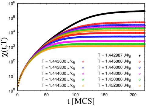
Figure 1: Simulation-time dependence of the magnetic susceptibility for $L=560$ at $T_{\rm c}$ and various temperatures used for the temperature scaling in the SW algorithm. The susceptibility decreases monotonically as the temperature increases.

First, we verify the temperature scaling in cluster algorithms (5) with the Swendsen-Wang (SW) algorithm. Here we concentrate on the magnetic susceptibility, i.e. $Q(t,T)\to\chi(t,T)$ and $x_{Q}\to\gamma$ in Eq. (5). In our previous article to investigate the 3D Heisenberg model with the NE-ES based on the SW algorithm Nonomura16 , the maximum system size was $L=560$. Here we also take $L=560$ and $225$ Monte Carlo steps (MCS), and average $4\times 10^{4}$ random-number sequences (RNS). The raw data for various temperatures (from $T=1.4436J/k_{\rm B}$ to $1.4520J/k_{\rm B}$) are shown in Fig. 1, together with the data at the most probable value of the critical point, $T_{\rm c}=1.442987J/k_{\rm B}$ Nonomura16 . At $t=225$MCS, $\chi$ for $T=1.4436J/k_{\rm B}$ is about $1/6$ of that at $T=T_{\rm c}$, while that at $T=1.4520J/k_{\rm B}$ is about $1/40$ of that at $T=1.4436J/k_{\rm B}$. Although the range of temperature for scaling does not seem so wide, that of $\chi$ is actually wide enough. In general, the temperature range of scaling is determined by the system size in the vicinity of $T_{\rm c}$, and by the temperature itself far from $T_{\rm c}$. Although the present formulation is based on the diverging behavior $\chi(t=\infty,L=\infty,T)\sim(T-T_{\rm c})^{-\gamma}$ for $T\to T_{\rm c}$, the actual finite-size behavior is saturated with $\chi(t=\infty,L,T_{\rm c})\sim L^{\gamma/\nu}$, and the range of scaling near $T_{\rm c}$ increases as $L$ increases. On the other hand, as temperature becomes away from $T_{\rm c}$, the weight of the correction terms to scaling increases independently of $L$.

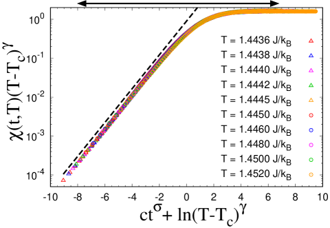
Figure 2: Temperature scaling plot of the data in Fig. 1 using $T_{\rm c}=1.442987J/k_{\rm B}$ and $\sigma=0.47$ Nonomura16 with $\gamma=1.3945(19)$ and $c=1.2595(43)$ in a semi-log scale. The arrow specifies the range of data used for the fitting, and the dashed line corresponds to a simple exponential curve as a guide for eyes. Here the data for $t=1$ MCS are not included.

These data are scaled with Eq. (5) in Fig. 2, namely the scaling plot of $\chi(t,T)(T-T_{\rm c})^{\gamma}$ versus $ct^{\sigma}+\ln(T-T_{\rm c})^{\gamma}$ in a semi-log scale using $T_{\rm c}=1.442987(2)J/k_{\rm B}$ and $\sigma=0.47(1)$ evaluated in Ref. Nonomura16 . Since we only take the data rather far away from $T_{\rm c}$, precise evaluation of $T_{\rm c}$ is difficult within the present scheme. It is also the case in the relaxation exponent $\sigma$. This exponent is characteristic to the critical relaxation in cluster algorithms, and appearance of it in Eq. (5) is just a trace of behaviors at $T_{\rm c}$. Then, it should be determined from the critical-relaxation data, not from the off-critical ones. The fitting parameters $\gamma$ and $c$ are estimated by minimizing the mutual residuals of these data. Although every two sets of the data can be scaled with each other, they are not independent and error bars cannot be evaluated in a simple way. Then, we average the mutual residuals between the nearest-neighbor temperatures, determine the range of fitting by minimizing the averaged residual as shown by arrows in Fig. 2, and obtain

$$\gamma=1.3945\pm 0.0019,\ c=1.2595\pm 0.0043.$$ (7)

Combining this estimate with $\gamma/\nu=1.972\pm 0.007$ obtained from the NE-ES at $T_{\rm c}$ Nonomura16 , we have

$$\nu=0.707\pm 0.003.$$ (8)

IV.2 Metropolis algorithm

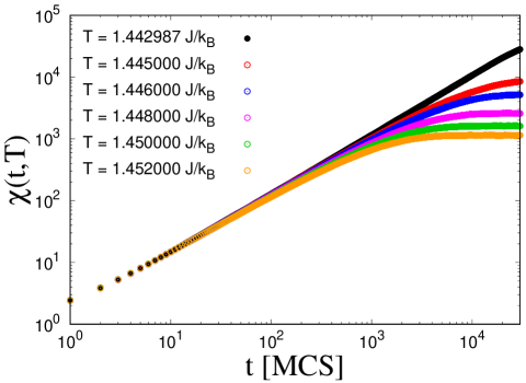
Figure 3: Simulation-time dependence of the magnetic susceptibility for $L=200$ at $T_{\rm c}$ Nonomura16 and various temperatures used for the temperature scaling in the Metropolis algorithm.

Next, we testify the temperature scaling in local-update algorithms (6) based on the Metropolis algorithm, and compare it with the standard off-critical scaling (3) for the same data. Here we also consider the magnetic susceptibility and take $Q(t,T)\to\chi(t,T)$ and $x_{Q}\to\gamma$ in these formulas. We take $L=200$ and $3\times 10^{4}$ MCS, and average $2\times 10^{4}$ RNS. The raw data at $T_{\rm c}$ Nonomura16 and for various temparatures (from $T=1.445J/k_{\rm B}$ to $1.452J/k_{\rm B}$) in a log-log scale in Fig. 3. Since the power-law relaxation at $T_{\rm c}$ is much slower than the stretched-exponential critical relaxation in the SW algorithm, much longer MCS are required and therefore the system size is reduced. The data at $T_{\rm c}$ still show a power-law behavior at $t=3\times 10^{4}$. When we attempt to evaluate $T_{\rm c}$ with the conventional NER, relaxation data at $T=1.443J/k_{\rm B}$ cannot be distinguished from the present data at $T_{\rm c}$, and the resolution of $T_{\rm c}$ becomes of one order lower than the one in Ref. Nonomura16 . In comparison with the previous subsection, the lowest temperature for scaling is increased in response to reduction of the system size, and the highest one is the same.

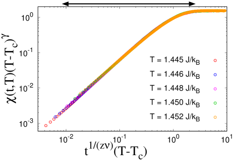
Figure 4: Temperature scaling plot of the data in Fig. 3 using $T_{\rm c}=1.442987J/k_{\rm B}$ Nonomura16 with $\gamma=1.4039(32)$ and $z\nu=1.4866(64)$ in a log-log scale. The arrow specifies the range of data used for the fitting. Here the data for $t=1,2$ MCS are not included.

These data are scaled with Eq. (6) in Fig. 4, namely the scaling plot of $\chi(t,T)(T-T_{\rm c})^{\gamma}$ versus $t^{1/(z\nu)}(T-T_{\rm c})$ in a log-log scale using $T_{\rm c}=1.442987(2)J/k_{\rm B}$ Nonomura16 . The fitting parameters $\gamma$ and $z\nu$ are estimated by minimizing the mutual residuals of these data. Since the relaxation process is much slower than that in the previous subsection, the number of data is further increased. When all the data are scaled with an equal weight, the contribution in the vicinity of equilibrium becomes dominant and the functional form in the whole simulation-time regions cannot be reproduced anymore. Then, we reduce the density of data as sparse as that for $51\sim 100$ MCS in a log scale by averaging the sequential data points. That is, we take $100$ points for $1\sim 100$ MCS, $50$ points for $101\sim 200$ MCS, $60$ points for $201\sim 500$ MCS, $50$ points for $501\sim 1,000$ MCS, $50$ points for $1,001\sim 2,000$ MCS, $60$ points for $2,001\sim 5,000$ MCS, $50$ points for $5,001\sim 10,000$ MCS, $50$ points for $10,001\sim 20,000$ MCS, and $20$ points for $20,001\sim 30,000$ MCS; totally we take $490$ points for $1\sim 30,000$ MCS for the fitting. Based on these set of data and the fitting scheme similarly to that in the previous subsection, we have

$$\gamma=1.4039\pm 0.0032,\ z\nu=1.4866\pm 0.0064.$$ (9)

Combining this estimate with $\nu$ in Eq. (8), we arrive at

$$z=2.10\pm 0.01.$$ (10)

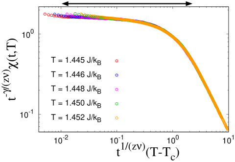
Figure 5: Off-critical scaling plot of the data in Fig. 3 based on the DFSS using $T_{\rm c}=1.442987J/k_{\rm B}$ Nonomura16 with $\gamma=1.4024(57)$ and $z\nu=1.4773(67)$ in a log-log scale. The arrow specifies the range of data used for the fitting. Here the data for $t=1\sim 3$ MCS are not included.

Finally, we analyze the same data (those in Fig. 3 after the above thinning-out process) with the standard off-critical scaling (3), namely the scaling plot of $t^{-\gamma/(z\nu)}\chi(t,T)$ versus $t^{1/(z\nu)}(T-T_{\rm c})$ as shown in Fig. 5. Using $T_{\rm c}=1.442987(2)J/k_{\rm B}$ Nonomura16 and the above fitting scheme, we have

$$\gamma=1.4024\pm 0.0057,\ z\nu=1.4773\pm 0.0067.$$ (11)

Combining this estimate with $\nu$ in Eq. (8), we obtain

$$z=2.09\pm 0.01.$$ (12)

V Discussion

According to the most precise evaluation of the critical exponents of the 3D Heisenberg model until present Campostrini02 , the exponents treated in the present article were given by $\gamma=1.3957(22)$ and $\nu=0.7113(11)$ by equilibrium Monte Carlo simulations. Our estimate of $\gamma$ based on the SW algorithm (7) is comparable with this one. Although ours of $\nu$ (8) is rather underestimated, it is still within the error bar. Note that this tendency is not due to the present analysis, but the one based on the NE-ES at $T_{\rm c}$, $\gamma/\nu=1.972(7)$ Nonomura16 . From the estimates in Ref. Campostrini02 , it is given by $\gamma/\nu=1.962(4)$, and the underestimation of $\nu$ simply originates from the overestimation of $\gamma/\nu$. Actually, in Ref. Campostrini02 the above MC analysis was coupled with the high-temperature expansion analysis, and they obtained more precise estimates $\gamma=1.3960(9)$ and $\nu=0.7112(5)$. Our estimate of $\gamma$ is still consistent with it, even though it is rather underestimated.

The tendency of underestimation can be understood from the finite-size behavior of physical quantities in the vicinity of equilibrium. As explained in the previous section, the temperature scaling is based on the diverging behavior of physical quantities, e.g. $\chi(T)\sim(T-T_{\rm c})^{-\gamma}$ for $T\to T_{\rm c}$. However, such a behavior is only observed in the thermodynamic limit, and in finite systems it saturates as $\chi(L,T_{\rm c})\sim L^{\gamma/\nu}$ even at $T=T_{\rm c}$. Then, when the data too close to $T_{\rm c}$ in comparison with $L$ are taken for the fitting, those become smaller than the ones expected from Eq. (5), which results in the underestimation of $\gamma$. On the other hand, the data far from $T_{\rm c}$ does not converge as sharp as a power with respect to $T-T_{\rm c}$. When the data too far away from $T_{\rm c}$ are used for the fitting, those become larger than the ones expected from Eq. (5), which also causes the underestimation of $\gamma$.

Our estimate of $\gamma$ based on the temperature scaling in the Metropolis algorithm (9) is overestimated (it is consistent with the previous estimate within $2\sigma$). Although that based on the conventional off-critical scaling in the Metropolis algorithm (11) is consistent with the previous one, it is due to large error bars and the most probable value itself is comparable with the one in Eq. (9) and is also overestimated. Even in the data in the Metropolis algorithm, tendency of underestimation in the vicinity of equilibrium is the same as those in the SW algorithm, and this tendency of overestimation originates from the early-time nonequilibrium behavior. The dynamical critical exponent $z$ is specific to the power-law critical relaxation in local-update algorithms, and the present estimate (10) may be comparable with that in the 3D Ising model, $z=2.055(10)$ Ito00 . There were no previous studies on the dynamical critical behaviors in the 3D Heisenberg model, and we cannot argue this slight discrepancy in $z$ too seriously at present.

Although the temperature scaling holds both in the SW and Metropolis algorithms, combination with the SW algorithm seems much better in the present analysis. Much larger systems can be treated owing to faster relaxation, and therefore critical phenomena can be evaluated more precisely. Moreover, origin of the discrepancy from the previous estimate can be understood naturally. In addition, the temperature scaling can be compared with the conventional off-critical scaling in the Metropolis algorithm. While the two fitting parameters are separated in the temperature scaling, they are coupled in the conventional off-critical scaling. Then, the error bar becomes twice larger in the latter, even though the most probable value of the estimate is comparable.

In the present article, we proposed the following procedure to determine critical phenomena with the cluster NER scheme:

1. Determine $T_{\rm c}$ by the NE-ES on the magnetization and/or magnetic susceptibility.

2. Determine $\beta/\nu$ and $\gamma/\nu$ by the NE-ES together with the above $T_{\rm c}$.

3. Determine $\gamma$ by the temperature scaling using the above $T_{\rm c}$.

4. Evaluate other critical exponents through the scaling relations.

This is a minimum procedure, and precise evaluation of $\beta$ within the present scheme seems difficult at present, as explained in the Appendix. However, from the scaling relation $\alpha+2\beta+\gamma=2$ and the hyperscaling relation $2-\alpha=d\nu$, we have $2\beta/\nu+\gamma/\nu=d$. That is, evaluation of $\beta$ is actually not necessary for the study on critical phenomena. If the critical exponent $\nu$ can be estimated from the temperature scaling of the correlation length $\xi$, the universality class can be identified only with the present scheme. Nevertheless, precise evaluation of $T_{\rm c}$ is not possible within this scheme, and the NE-ES of the critical relaxation is indispensable for the cluster NER.

VI Summary

In the present article, we proposed a new scaling theory in the nonequilibrium relaxation process called as the temperature scaling, and we confirmed this theory on the magnetic susceptibility in the 3D Heisenberg model. When the temperature scaling was combined with the Swendsen-Wang (SW) algorithm, it worked very well and our estimate of the critical exponent $\gamma=1.3945(19)$ is comparable with the previous best estimate. When it was combined with the Metropolis algorithm, it worked as well as the conventional off-critical scaling, but not as well as the case with the SW algorithm, because of limitation of system sizes owing to slow relaxation.

Appendix A Magnetization in the SW algorithm

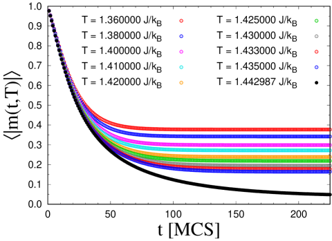
Figure 6: Simulation-time dependence of the absolute value of magnetization for $L=560$ at $T_{\rm c}$ and various temperatures in the SW algorithm. The magnetization decreases monotonically as the temperature increases.

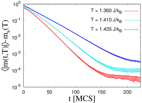
Figure 7: Simulation-time dependence of the decaying part of the absolute value of magnetization based on Eq. (13) in a semi-log scale at $T=1.360J/k_{\rm B}$, $1.410J/k_{\rm B}$ and $1.435J/k_{\rm B}$ (from bottom to top).

Even if Monte Carlo simulations are started from the perfectly-ordered state, the sign of magnetization may change in each step by a global flip of large clusters in the relaxation process in cluster algorithms. When the data of different random-number sequences are averaged, cancellation of signs takes place and the averaged results become meaningless. Then, in the cluster NER, we take the absolute value of magnetization. Here we start from the perfectly-ordered state, simulate the $L=560$ system during $225$ MCS with the SW algorithm, and average $4\times 10^{4}$ RNS. The relaxation data for various temperatures (from $T=1.360J/k_{\rm B}$ to $1.435J/k_{\rm B}$ and at $T_{\rm c}$) are displayed in Fig. 6.

Although the data at $T_{\rm c}$ decay on a stretched-exponential curve and do not arrive at equilibrium at $t=225$ MCS, other data for $T<T_{\rm c}$ seem to be already in equilibrium at that simulation time. Such relaxation behaviors are described by the following formula,

$$\langle|m(t,T)|\rangle=m_{\rm s}(T)+A(T)\exp(-C(T)t),$$ (13)

with the spontaneous magnetization $m_{\rm s}(T)$ and fitting parameters $A(T)$ and $C(T)$. This formula was confirmed in the 2D Ising model in the Wolff algorithm Nonomura14 , while the stretched-exponential relaxation was reported in the local-update algorithms Ito93 ; Stauffer96 . This relaxation formula is verified in Fig. 7 by fitting the data with Eq. (13) and plotting $\langle|m(t,T)|\rangle-m_{\rm s}(T)$ versus $t$ in a semi-log scale at $T=1.360J/k_{\rm B}$, $1.410J/k_{\rm B}$ and $1.435J/k_{\rm B}$ (from bottom to top). Linearity of the data reveals validity of Eq. (13), and variance of the initial value and slope of the data represents explicit temperature dependence of the parameters $A(T)$ and $C(T)$ in Eq. (13), respectively. Such nontrivial $T$-dependence other than that of $m_{\rm s}(T)$ makes a scaling analysis based on Eq. (13) difficult.

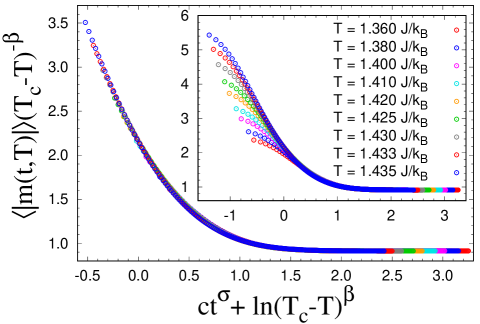
Figure 8: Temperature scaling plot of the data in Fig. 6 after $16$ MCS using $T_{\rm c}=1.442987J/k_{\rm B}$ and $\sigma=0.47$ Nonomura16 with $\beta=0.3553(10)$ and $c=0.3244(3)$. The plot including the relaxation data for the initial $15$ MCS is shown in the inset.

Nevertheless, the temperature scaling still holds on this quantity. From the stretched-exponential critical relaxation from the perfectly-ordered state, $\langle|m(t,T)|\rangle\sim\exp(-ct^{\sigma})$, and the temperature dependence in equilibrium, $\langle|m(t=\infty,T)|\rangle\sim(T_{\rm c}-T)^{\beta}$, we have

$$\langle|m(t,T)|\rangle\sim(T_{\rm c}-T)^{\beta}f_{\rm tsc}[ct^{\sigma}+\ln(T_{\rm c}-T)^{\beta}].$$ (14)

The data in Fig. 6 are scaled with Eq. (14) in Fig. 8. Although the initial-time data are not scaled well owing to the discrepancy with the exponential decay (13) as shown in the inset of Fig. 8, the scaling formula (14) actually holds very well for the data from $16$ MCS (in the main panel of Fig. 8). Similarly to the temperature scaling of the magnetic susceptibility, we minimize the mutual residuals of these data using $T_{\rm c}=1.442987(2)J/k_{\rm B}$ and $\sigma=0.47(1)$ Nonomura16 . We find that the averaged residuals are minimized when all the data in the main panel of Fig. 8 are used for the fitting, and we have

$$\beta=0.3553\pm 0.0010,\ c=0.3244\pm 0.0003.$$ (15)

Although the error bars seem small enough, this estimate is not consistent with the most precise estimate until present, $\beta=0.3689(3)$ Campostrini02 .

The background of this discrepancy can be explained by the evaluation of $\beta$ from the temperature dependence of $m_{\rm s}(T)$ in Eq. (13). Up to the leading term, it is given by $m_{\rm s}(T)=B_{1}(T_{\rm c}-T)^{\beta}$, and using all the data for $T<T_{\rm c}$ in Fig. 6, we have $\beta=0.3574(2)$. This estimate is not so different from that in Eq. (15), and not consistent with the one in Ref. Campostrini02 , neither. On the other hand, when we take the next-order term into account as

$$m_{\rm s}(T)=B_{1}(T_{\rm c}-T)^{\beta}+B_{2}(T_{\rm c}-T)^{2\beta},$$ (16)

we obtain

$$\beta=0.3691\pm 0.0010,$$ (17)

$$B_{1}=0.988\pm 0.005,\ B_{2}=-0.107\pm 0.007.$$ (18)

This estimate is consistent with the one in Ref. Campostrini02 , and the coefficient of the next-order term is about $10\%$ of that of the leading term. These results tell that the next-order term is crucial for the description of the critical phenomena in the 3D Heisenberg model based on the temperature dependence of the magnetization, and that the temperature-scaling formalism based only on the leading term of the temperature dependence of physical quantities is not suitable for the magnetization, at least in the present model. This mechanism is independent of the update algorithms, and therefore we do not consider the Metropolis algorithm here.

References

- (1) As a review article, Y. Ozeki and N. Ito, J. Phys. A: Math. Theor. 40, R149 (2007).
- (2) M. Suzuki, Phys. Lett. A 58, 435 (1976); Prog. Theor. Phys. 58, 1142 (1977).
- (3) P. C. Hohenberg and B. I. Halperin, Rev. Mod. Phys. 49, 435 (1977).
- (4) R. H. Swendsen and J.-S. Wang, Phys. Rev. Lett. 58, 86 (1987).
- (5) U. Wolff, Phys. Rev. Lett. 62, 361 (1989); Nucl. Phys. B 322, 759 (1989).
- (6) Y. Nonomura, J. Phys. Soc. Jpn. 83, 113001 (2014).
- (7) Y. Nonomura and Y. Tomita, Phys. Rev. E 92, 062121 (2015).
- (8) Y. Nonomura and Y. Tomita, Phys. Rev. E 93, 012101 (2016).
- (9) Y. Nonomura and Y. Tomita, Phys. Rev. E 101, 032105 (2020).
- (10) Y. Tomita and Y. Nonomura, Phys. Rev. E 98, 052110 (2018).
- (11) F. Y. Wu, Rev. Mod. Phys. 54, 235 (1982).
- (12) M. Campostrini, M. Hasenbusch, A. Pelissetto, P. Rossi, and E. Vicari, Phys. Rev B 65, 144520 (2002).
- (13) N. Ito, K. Hukushima, K. Ogawa, and Y. Ozeki, J. Phys. Soc. Jpn. 69, 1931 (2000).
- (14) N. Ito, Physica A 192, 604 (1993); ibid. 196, 591 (1993).
- (15) P. Grassberger and D. Stauffer, Physica A 232, 171 (1996); D. Stauffer, Physica A 244, 344 (1997).
- (16) M. Matsumoto and T. Nishimura, ACM TOMACS 8, 3 (1998); the Mersenne Twister Home Page maintained by M. Matsumoto, http://www.math.sci.hiroshima-u.ac.jp/~m-mat/MT/emt.html