Thermodynamics of interacting single-domain superparamagnetic nanoparticles frozen in the nodes of a regular cubic lattice

Abstract

In this work, we study the effect of dipole-dipole interparticle interactions on the static thermodynamic and magnetic properties of an ensemble of immobilized monodisperse superparamagnetic nanoparticles. We assume that magnetic nanoparticles are embedded in the nodes of a regular cubic lattice, so that the particle translational degrees of freedom are turned off. The relaxation of the magnetic moments of the nanoparticles occurs by the Néel mechanism. The easy axes are aligned (i) parallel or (ii) perpendicular to the direction of an external field. These models are investigated using theory and computer simulation, taking microscopic discrete structure explicitly into account. The analytical expressions of the Helmholtz free energy, the static magnetization, and the initial magnetic susceptibility are derived for both configurations (i) and (ii) as functions of the height of the magnetic crystallographic anisotropy energy barrier, measured by parameter $\sigma$, and the intensity of the dipole-dipole interparticle interactions measured by $\lambda_{e}$. A good agreement between the theory and the results of MC simulations in the region of low and moderate values of $\lambda_{e}$ and $\sigma$ is obtained. For high values of $\lambda_{e}$ and $\sigma$, the structuring of magnetic moments in regularly orientated structures was found from MC simulations for configuration (i).

I Introduction

Smart materials, also called responsive or intelligent materials, are special materials that have one or more properties that can be significantly changed in a controlled fashion by external stimuli, for example a magnetic field. Such materials include magnetic composites, which are produced by embedding magnetic nanoparticles in a liquid or polymer matrix. Examples of these composites are ferrofluids, magnetic elastomers, ferrogels, magnetic emulsions, and various biocompatible magnetic fillings Kuznetsova et al. (2019); Borin et al. (2019); Filipcsei et al. (2007); Blyakhman et al. (2019). Today, such materials are widely used in various medical applications because they actively respond to applied magnetic fields. For example, they are an indispensable tool in magnetic hyperthermia, in which the micromotions of magnetic nanoparticles in an alternating magnetic field leads to the heating and destruction of tumor cells Dutz and Hergt (2013); Ortega and Pankhurst (2013); Zubarev (2018, 2019); Zhang et al. (2017); Piehler et al. (2020); Brero et al. (2020). The response of the magnetic composites to the applied magnetic field is determined by two main physical mechanisms of the magnetic moment’s orientational relaxation in nanosized particles. They are the Brownian rotation of particles with fixed magnetic moments and the superparamagnetic Néel rotation of magnetic moments inside the particles due to thermal fluctuations Raikher and Shliomis (1974); Shliomis and Stepanov (1994). For ensembles of nanoparticles suspended in some liquid carriers, known as ferrofluids, both mechanisms take place. But when nanoparticles are embedded in a polymer matrix or biological tissues, the particles often lose their translational and orientational freedom. In this case, the superparamagnetic Néel relaxation becomes the major mechanism determining the magnetic properties of the ensembles of such immobilized nanoparticles.

Today there are many established synthesis techniques that make it possible to generate a magnetic composite with various nano- and microscopic architectures Gervald et al. (2010); Valiev et al. (2019); Ganesan et al. (2019); Filipcsei et al. (2007); Weeber et al. (2018); Tanasa et al. (2019); Bastola et al. (2020). A different distribution of magnetic nanoparticles inside the sample leads to a significant change in its bulk properties Zakinyan and Arefyev (2020); Yoshida et al. (2017); Elfimova et al. (2019). In addition, interparticle dipole-dipole interactions have a strong effect on the macroproperties of the system, and this is manifested differently in liquid or polymer based composites. So, strong interparticle dipole-dipole interactions lead to aggregation in the ferrofluid Socoliuc and Popescu (2020); Elkady et al. (2015); Pshenichnikov and Ivanov (2012); Daffé et al. (2020), whereas in the system of immobilized magnetic nanoparticles, interparticle interactions can only be a cause of the structuring of the magnetic moments of the nanoparticles, since the particles themselves remain stationary Ilg (2017); Pshenichnikov and Kuznetsov (2015); Solovyova et al. (2020). The effects of dipole-dipole interactions on the bulk properties of ferrofluids are well understood theoretically Elfimova et al. (2017); Ivanov and Camp (2018); Solovyova et al. (2017); Minina et al. (2018); Szalai et al. (2013), experimentally Nagornyi et al. (2020); Lebedev et al. (2019); Linke and Odenbach (2015); Daffé et al. (2020), and by computer simulation methods Minina et al. (2018); Pousaneh and De Wijn (2020); Ivanov and Camp (2018); Solovyova et al. (2017); Szalai et al. (2013); Daffé et al. (2020). However, devising a theory that takes into account dipole-dipole interactions in a system of immobilized superparamagnetic nanoparticles still remains a challenge.

In recent works, the magnetic response of a system of immobilized interacting single-domain nanoparticles distributed randomly Elfimova et al. (2019) or placed at the nodes of a simple cubic lattice Solovyova et al. (2020) within an implicit solid matrix was investigated using statistical-mechanical theory and computer simulations. In the first work Elfimova et al. (2019), superparamagnetic particles with uniaxial magnetic anisotropy were considered. The relaxation of the magnetic moments of particles occurred by the Néel mechanism. The easy axes were distributed according to the particular textures: aligned parallel or perpendicular to the external magnetic field, or randomly distributed. The initial magnetic susceptibility was found to depend on the magnetic crystallographic anisotropy barrier (measured with respect to thermal energy by a parameter $\sigma$) in very different ways for various textures. The initial susceptibility increased as $\sigma$ for a parallel texture, while with a perpendicular texture, the initial susceptibility decreased. With a random distribution, the initial susceptibility was independent of $\sigma$. In all cases, interactions between nanoparticles led to an enhancement of the initial susceptibility, but the enhancement was much stronger for the parallel texture than for the perpendicular or random textures. In the second work Solovyova et al. (2020), it was assumed that nanoparticles are embedded in the nodes of the simple cubic lattice (SCLF) and the relaxation of the magnetic moments of nanoparticles occurs by the Brownian mechanism. The particles had no intrinsic magnetic anisotropy, but could rotate on the lattice nodes under the influence of the external magnetic field and as a result of the interparticle dipolar interactions. The magnetic properties of SCLF were compared with ones for a ferrofluid, modeled by a system of dipole hard spheres (DHS). It was found that at low intensities of the dipole-dipole interactions, the magnetization of DHS and SCLF is the same. For strong and moderate dipolar coupling regimes and with a weak magnetic field, the magnetization of the DHS system is higher than the magnetization of SCLF, while the opposite tendency is observed at stronger fields. The reasons of this behavior were discussed in the article Solovyova et al. (2020).

These two works Elfimova et al. (2019); Solovyova et al. (2020) demonstrated how different distributions of magnetic nanoparticles within a sample can change its macroproperties. Nevertheless, the theory is still incomplete and the topic is not fully understood. The question of how the internal magnetic anisotropy of nanoparticles affects the properties of SCLF remains unclear. The aim of this work is to fill this gap. The properties of a monodisperse system of immobilized interacting single-domain spherical nanoparticles, with uniaxial magnetic anisotropy, placed at the nodes of a simple cubic lattice will be studied in the current work using a statistical-mechanical approach and computer simulations.

This article is arranged as follows. In Sec. II, the theory and simulation methods are detailed, and new analytical approximations for the Helmholtz free energy are derived. The main results are presented as a comparison between theory and simulation in Sec. III. The conclusions from the work are summarized in Sec.IV.

II Model and methods

II.1 Model

The sample under consideration consists of $N$ immobilized superparamagnetic spherical nanoparticles distributed regularly on simple cubic lattice nodes with period a. All particles have the same magnetic-core diameter $x$ and magnetic moment $m=v_{m}M_{s}$, where $M_{s}$ is the bulk saturation magnetization, $v_{m}=\pi x^{3}/6$ is the magnetic core volume. The radius vector and magnetic moment of nanoparticle $i$ are $\textbf{r}_{i}=r_{i}\hat{\textbf{r}}_{i}$ and $\bm{m}_{i}=m_{i}\bm{\Omega}_{i}$ respectively, where $\hat{\textbf{r}}_{i}=(\sin\theta_{i}\cos\phi_{i},\sin\theta_{i}\sin\phi_{i},\cos\theta_{i})$ and $\bm{\Omega}_{i}=(\sin\omega_{i}\cos\xi_{i},\sin\omega_{i}\sin\xi_{i},\cos\omega_{i})$ are unit vectors.

The magnetic moment of a nanoparticle has two degenerate ground-state directions, these being parallel and anti-parallel to the easy axis, denoted by vector $\textbf{n}_{i}$. The Néel energy $U_{N}$ as a function of the angle between $\textbf{m}_{i}$ and $\textbf{n}_{i}$ is given by

$$U_{N}(i)=-Kv_{m}(\bm{\Omega}_{i}\cdot\hat{\textbf{n}}_{i})^{2},$$ (1)

where $\hat{\textbf{n}}_{i}$ is a unit vector and $K$ is the magnetic crystallographic anisotropy constant (a material property).

The interaction between magnetic moment $\textbf{m}_{i}$ and uniform external magnetic field H is described by the Zeeman energy

$$U_{m}(i)=-\mu_{0}(\textbf{m}_{i}\cdot\textbf{{H}})=-\mu_{0}mH(\bm{\Omega}_{i}\cdot\hat{\textbf{{h}}}),$$ (2)

where it is assumed that the applied magnetic field H has the strength $H$ and the orientation $\hat{\textbf{{h}}}$.

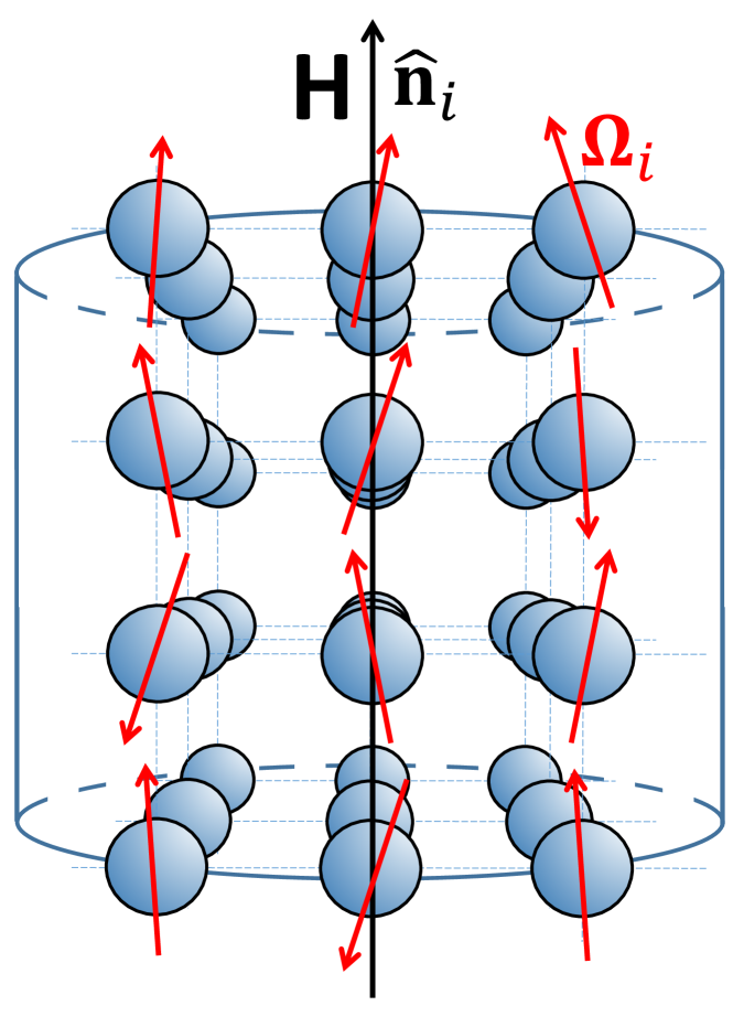
(a)

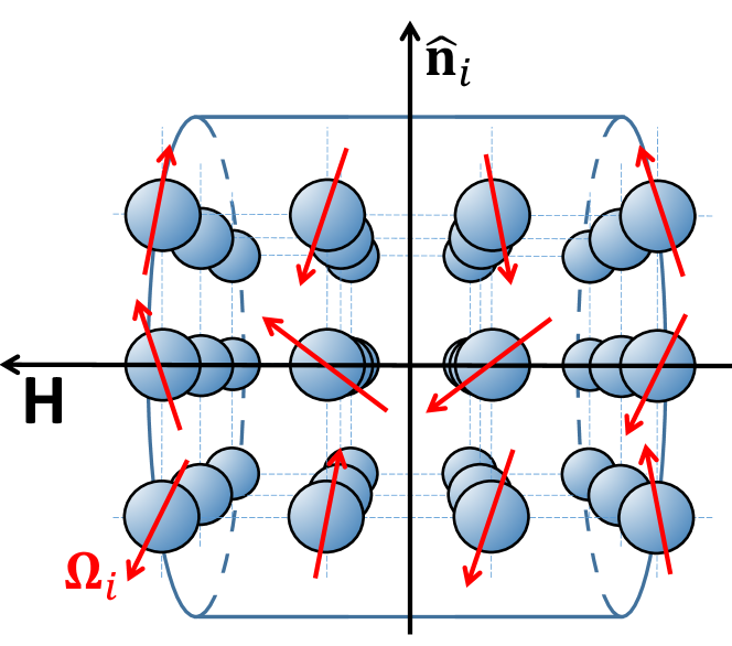
(b)

Figure 1: Monodisperse system of immobilized single-domain superparamagnetic nanoparticles placed on the nodes of a simple cubic lattice at external magnetic field for (a) parallel and (b) perpendicular configurations.

The pair dipole-dipole interaction of the two particles i and j obeys to the anisotropic potential $U_{d}$

$$U_{d}(ij)=\frac{\mu_{0}m^{2}}{4\pi r_{ij}^{3}}\Big{[}(\bm{\Omega}_{i}\cdot\bm{\Omega}_{j})-3(\bm{\Omega}_{i}\cdot\hat{\textbf{r}}_{ij})(\bm{\Omega}_{j}\cdot\hat{\textbf{r}}_{ij})\Big{]},$$ (3)

where $\textbf{r}_{ij}=r_{ij}\hat{\textbf{r}}_{ij}=\textbf{r}_{j}-\textbf{r}_{i}$ has the meaning of a center-center separation vector with the length $r_{ij}=|\textbf{r}_{ij}|$.

The total potential energy normalized by the thermal energy $k_{B}T=\beta^{-1}$ has the following form

$$\beta U = \beta\sum_{j>i=1}^{N}U_{d}(ij)-\sigma\sum_{i=1}^{N}(\bm{\Omega}_{i}\cdot\hat{\textbf{n}}_{i})^{2}-\alpha\sum_{i=1}^{N}(\bm{\Omega}_{i}\cdot\hat{\textbf{h}}),$$ (4)

where the dimensionless anisotropy parameter $\sigma=\beta v_{m}K$ and the Langevin parameter $\alpha=\beta\mu_{0}mH$ are introduced. The relationship between the pair magnetic interaction and the thermal energy is measured by the effective dipolar coupling constant $\lambda_{e}$

$$\lambda_{e}=\frac{\mu_{0}m^{2}\beta}{4\pi a^{3}},$$ (5)

the definition of which takes into account that two nanoparticles located in the nodes of the simple cubic lattice can not be closer than the lattice period $a\geq x$ .

Two types of orientational distributions of the easy axes will be considered: aligned (i) parallel and (ii) perpendicular to the direction of the external field H. To simplify the analytical calculations, the easy axes of both configuration are assumed to be aligned along the laboratory $Oz$ axis, namely $\hat{\textbf{n}}_{i}=(0,0,1)$, so the Néel energy can be represented as

$$U_{N}(i)=-\sigma\cos^{2}\omega_{i}.$$ (6)

The direction of external magnetic field H is set (i) $\textbf{H}=H(0,0,1)$ in parallel configuration so that

$$U_{m}^{||}(i)=-\alpha\cos\omega_{i}$$ (7)

and (ii) $\textbf{H}=H(1,0,0)$ in perpendicular configuration so

$$U_{m}^{\perp}(i)=-\alpha\sin\omega_{i}\cos\xi_{i}.$$ (8)

For vanishing of demagnetization fields, we will assume that the sample container has a long cylindrical shape elongated in the direction of an external magnetic field H. The sample geometries studied in this work are given in Fig. 1.

II.2 The Helmholtz Free Energy of an ensemble of immobilized nanoparticles

II.2.1 Ideal system

The definition of the Helmholtz free energy $F$ contains the configurational integral $Z$ so, that

$$\beta F=-\ln\left(Z\right).$$ (9)

To extract the contribution of the dipole-dipole interactions, it is convenient to split the Helmholtz free energy $F$ into two parts

$$F=F_{\textrm{\scriptsize{id}}}+\Delta F.$$ (10)

The first term corresponds to the ideal system of superparamagnetic non-interacting nanoparticles in the applied magnetic field, the configurational integral $Z_{id}$ of which is

$$\beta F_{\textrm{\scriptsize{id}}} = -\ln\left(Z_{\textrm{\scriptsize{id}}}\right),$$ (11)

$$Z_{\textrm{\scriptsize{id}}} = \prod\limits_{k=1}^{N}\int p(\textbf{r}_{k})d\textbf{r}_{k}d\bm{\Omega}_{k}$$ (12)

$$\times \exp\left(\sum\limits_{i=1}^{N}\big{[}\alpha(\bm{\Omega}_{i}\cdot\hat{\textbf{h}})+\sigma\cos^{2}\omega_{i}\big{]}\right),$$

$$d\textbf{r}_{k} = r_{k}^{2}\sin\theta_{k}dr_{k}d\theta_{k}d\phi_{k},$$ (13)

$$d\bm{\Omega}_{k} = \frac{1}{4\pi}\sin\omega_{k}d\omega_{k}d\xi_{k}.$$ (14)

In this definition, $p(\textbf{r}_{k})$ describes the probability of the location of nanoparticle k at a given point in the volume

$$p(\textbf{r}_{k})=\delta(\textbf{r}_{k}-\textbf{r}_{k}^{(0)}).$$ (15)

The ’lattice position’ of nanoparticle $\textbf{r}_{k}^{(0)}$ may obey to a regular or a random law. For both cases, the normalization rule is

$$\int p(\textbf{r}_{k})d\textbf{r}_{k}=1.$$ (16)

Therefore in the integrand function of Eq. (12), there are no dependencies on nanoparticle positions. With this integration, all nanoparticles are equivalent to each other. This allows us to rewrite $Z_{\textrm{\scriptsize{id}}}$ as follows

$$Z_{\textrm{\scriptsize{id}}}=\left(\int d\bm{\Omega}_{1}\exp\left[\alpha(\bm{\Omega}_{1}\cdot\hat{\textbf{h}})+\sigma\cos^{2}\omega_{1}\right]\right)^{N},$$ (17)

the result of which can be calculated numerically for each set of parameters $\alpha$ and $\sigma$ and the fixed direction of vector $\hat{\textbf{n}}_{1}$. It worth be stressed that the Helmholtz free energy of an ideal system

$$\frac{\beta F_{\textrm{\scriptsize{id}}}}{N}=-\ln\left(\int d\bm{\Omega}_{1}\exp\left[\alpha(\bm{\Omega}_{1}\cdot\hat{\textbf{h}})+\sigma\cos^{2}\omega_{1}\right]\right)\ \$$ (18)

does not depend on parameter $\lambda$, which characterizes the dipole-dipole interparticle interactions.

II.2.2 A system with interparticle dipole-dipole interactions

The second term $\Delta F$ in (10) corresponds to the contribution of dipole-dipole correlations in the Helmholtz free energy

$$\beta\Delta F = -\ln\left(\frac{Z}{Z_{\textrm{\scriptsize{id}}}}\right),$$ (19)

$$\frac{Z}{Z_{\textrm{\scriptsize{id}}}} = \frac{1}{Z_{\textrm{\scriptsize{id}}}}\prod\limits_{k=1}^{N}\int p(\textbf{r}_{k})d\textbf{r}_{k}d\bm{\Omega}_{k}\exp\Bigg{(}-\sum\limits_{j>i=1}^{N}\beta U_{d}(ij)$$ (20)

$$+ \sum\limits_{i=1}^{N}\big{[}\alpha(\bm{\Omega}_{i}\cdot\hat{\textbf{h}})+\sigma\cos^{2}\omega_{i}\big{]}\Bigg{)},$$

where Z is the configurational integral of the SCLF, including dipole-dipole interaction. Introducing Boltzmann-weighted averaging over the magnetic moment orientation of nanoparticle k

$$d\bm{\Psi}_{k}=\frac{d\bm{\Omega}_{k}\exp\left[\alpha(\bm{\Omega}_{k}\cdot\hat{\textbf{h}})+\sigma\cos^{2}\omega_{k}\right]}{\int d\bm{\Omega}_{1}\exp\left[\alpha(\bm{\Omega}_{1}\cdot\hat{\textbf{h}})+\sigma\cos^{2}\omega_{1}\right]},$$ (21)

one can rewrite definition (20) in a more compact form

$$\frac{Z}{Z_{\textrm{\scriptsize{id}}}} = \prod\limits_{k=1}^{N}\int p(\textbf{r}_{k})d\textbf{r}_{k}d\bm{\Psi}_{k}\prod\limits_{j>i=1}^{N}(1+f_{ij}),$$ (22)

$$f_{ij} = \exp\left(-\beta U_{d}(ij)\right)-1,$$ (23)

where $f_{ij}$ is the Mayer function. This approach reproduces the method of Solovyova et al. (2020), which was developed for $\sigma\equiv 0$. The main difference is the definition of the Boltzmann-weighted integration $d\bm{\Psi}_{k}$ (21), which in our case also depends on the anisotropy parameter $\sigma\geq 0$ and coincides with the same from Solovyova et al. (2020) for $\sigma=0$. Therefore, it is possible to apply the final results for the configurational part of the Helmholtz free energy from Solovyova et al. (2020) to our system with the new definition of operator $d\bm{\Psi}_{k}$:

$$\frac{\beta\Delta F}{N} = -\frac{1}{2}\sum\limits_{j=2}^{N}\left\langle f_{1j}^{(0)}\right\rangle.$$ (24)

where $f_{1j}^{(0)}=\int p(\textbf{r}_{1})d\textbf{r}_{1}\int p(\textbf{r}_{j})d\textbf{r}_{j}f_{1j}$ is the Mayer function of the nanoparticles 1 and j in their ’lattice positions’. The angle brackets in (24) denote a Boltzmann-weighted integration (21) over the orientation of both nanoparticles 1 and j

$$\left\langle f_{1j}^{(0)}\right\rangle=\int f_{1j}^{(0)}d\bm{\Psi}_{1}d\bm{\Psi}_{j}.$$ (25)

It should be emphasized that approximation (24) is obtained due to the logarithm expansion of (19) up to the linear term, and it is limited by the second virial coefficient level, which means the consideration of the interparticle interactions in nanoparticle pairs only.

This definition of $\Delta F$ is valid for the regular types of nanoparticle distribution in the system volume, such as SCLF or other lattices. For the random distribution of magnetic nanoparticles in the sample volume, it is necessary to average (24) over all possible random configurations. This means that in the limit, every particle $j$ in sum of (24) can occupy any position in the sample volume except for that of particle 1:

$$\frac{\beta\Delta F^{\textrm{random}}}{N} = -\frac{1}{2}\sum\limits_{j=2}^{N}\int\frac{dr_{1j}}{V}\left\langle f_{1j}\right\rangle$$

$$= -\frac{N}{2V}\int dr_{12}\left\langle f_{12}\right\rangle=\rho B_{2},$$

where $\rho=N/V$ is nanoparticle density, $B_{2}$ corresponds the classical definition of the second virial coefficient in the theory of liquids Balescu (1975).

Next we will consider in detail the behavior of SCLF. The Mayer function (23) is expanded in a series up to the third order in terms of the dipolar energy $U_{d}$

$$f_{1j}^{(0)}=-\beta U_{d}(1j)+\frac{\left[-\beta U_{d}(1j)\right]^{2}}{2!}+\frac{\left[-\beta U_{d}(1j)\right]^{3}}{3!}.\ \ \ \$$ (27)

Dipole-dipole potential $U_{d}$ includes the dependencies over both the translational and orientational degrees of freedom of nanoparticles 1 and j. Applying the Boltzmann-weighted integration over the magnetic moment orientations $\textbf{m}_{1}$ and $\textbf{m}_{j}$, it is possible to represent the value of $\beta\Delta F$ in the common form

$$\frac{\beta\Delta F}{N} = -\frac{1}{2}\left(b_{1}\lambda_{e}+b_{2}\lambda_{e}^{2}+b_{3}\lambda_{e}^{3}\right),$$ (28)

$$b_{1} = \sum\limits_{j=2}^{N}\bigg{\langle}\frac{-\beta U_{d}(1j)}{\lambda_{e}}\bigg{\rangle},$$ (29)

$$b_{2} = \sum\limits_{j=2}^{N}\bigg{\langle}\frac{1}{2!}\left(\frac{-\beta U_{d}(1j)}{\lambda_{e}}\right)^{2}\bigg{\rangle},$$ (30)

$$b_{3} = \sum\limits_{j=2}^{N}\bigg{\langle}\frac{1}{3!}\left(\frac{-\beta U_{d}(1j)}{\lambda_{e}}\right)^{3}\bigg{\rangle}.$$ (31)

The coefficients $b_{1}$, $b_{2}$ and $b_{3}$ are different for the parallel and perpendicular configurations and will be discussed separately.

II.3 The parallel configuration of SCLF with superparamagnetic nanoparticles

The parallel configuration corresponds to Fig. 1 (a), which means $(\bm{\Omega}_{i}\cdot\hat{\textbf{h}})=(\bm{\Omega}_{i}\cdot\hat{\textbf{n}}_{i})=\cos\omega_{i}$. In this case, the ideal part of the Helmholtz free energy (18) is equal to

$$\frac{\beta F_{\textrm{\scriptsize{id}}}}{N}=-\ln\left[Q_{0}(\alpha,\sigma)\right],$$ (32)

where

$$Q_{0}(\alpha,\sigma) = \frac{1}{2}\int\limits_{-1}^{1}\exp\left(\alpha t+\sigma t^{2}\right)dt,$$ (33)

$$Q_{0}(\alpha,0) = \frac{\sinh{\alpha}}{\alpha}.$$ (34)

The Boltzmann-weighted integration over the orientation of the nanoparticle magnetic moments for the parallel configuration is

$$d\bm{\Psi}_{k}=\frac{d\bm{\Omega}_{k}\exp\left(\alpha\cos\omega_{k}+\sigma\cos^{2}\omega_{k}\right)}{Q_{0}(\alpha,\sigma)}.$$ (35)

Details of the averaging of coefficients $b_{1}$, $b_{2}$, $b_{3}$ over magnetic moment orientations and particle positions are provided in Appendix A. The final analytical expression for $\Delta F$ expansion can be presented as

$$\frac{\beta\Delta F}{N} = -2.0944Q_{1}^{2}(\alpha,\sigma)\lambda_{e}$$ (36)

$$- \left[1.9390Q_{2}^{2}(\alpha,\sigma)+1.4003\right]\lambda_{e}^{2}$$

$$- \big{[}0.1611Q_{3}^{2}(\alpha,\sigma)+1.5595Q_{1}(\alpha,\sigma)Q_{3}(\alpha,\sigma)$$

$$- 0.7285Q_{1}^{2}(\alpha,\sigma)\big{]}\lambda_{e}^{3},$$

where additional functions $Q_{k}(\alpha,\sigma)$ are defined in Appendix A. It is well known that the virial expansion for a system with dipole-dipole interactions is an alternating series Henderson (2011); Joslin (1981), and therefore it is very sensitive to truncation of the series. Hence, it could be more efficient to transform the virial expansion of the Helmholtz free energy (36) back into the logarithmic form (19):

$$\frac{\beta\Delta F}{N} = -\ln\Big{\{}1+2.0944Q_{1}^{2}(\alpha,\sigma)\lambda_{e}$$ (37)

$$+ \left[1.9390Q_{2}^{2}(\alpha,\sigma)+1.4003\right]\lambda_{e}^{2}$$

$$+ \big{[}0.1611Q_{3}^{2}(\alpha,\sigma)+1.5595Q_{1}(\alpha,\sigma)Q_{3}(\alpha,\sigma)$$

$$- 0.7285Q_{1}^{2}(\alpha,\sigma)\big{]}\lambda_{e}^{3}\Big{\}},$$

so that the terms from the right-hand side of Eq. (36) are the first terms of the Maclaurin expansion of the logarithm in (37). The advantage of the logarithmic form is that the logarithm of a polynomial is less sensitive to polynomial truncation at the low order in $\lambda_{e}$-expansion. First suggested in Elfimova et al. (2012), this method allows for the expansion of the theory applicability over both the volume nanoparticle concentration and the dipolar coupling constant for the prediction of the properties of the dipolar hard sphere fluid Elfimova et al. (2013); Solovyova et al. (2020); Solovyova and Elfimova (2020). The typical behavior of the dipole-dipole contribution in the Helmholtz free energy $\Delta F$ as a function of the anisotropy parameter $\sigma$ is shown in Fig. 2 with $\alpha=0$, 1, 2, and 5, and a rather high value of intensity of dipole-dipole interactions $\lambda_{e}=0.5$. For $0\leq\sigma\leq 5$, one can note that the contribution $\Delta F$ increases more rapidly than for $\sigma>5$.

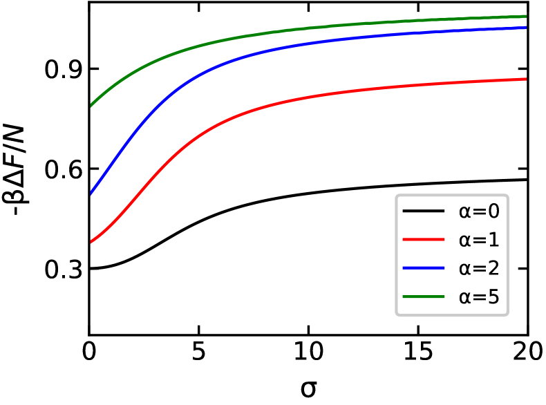
Figure 2: The contribution of dipole-dipole interactions $\Delta F$ for the parallel configuration as a function of the anisotropy parameter $\sigma$ for the system with $\lambda_{e}=0.5$ and different values of $\alpha$ = 0, 1, 2 , and 5. The value of $\alpha$ increases from the bottom to the top.

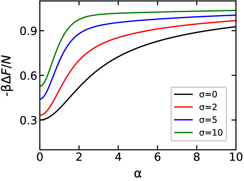
Figure 3: The contribution of dipole-dipole interactions $\Delta F$ for the parallel configuration as a function of the Langevin parameter $\alpha$ for the system with $\lambda_{e}=0.5$ and different values of $\sigma$ = 0, 2, 5 and 10. The value of $\sigma$ increases from the bottom to the top.

In the parallel configuration, anisotropy axes are an addition stimulus to the alignment of magnetic moments along the external magnetic field, which leads an increase in the Helmholtz free energy as the anisotropy parameter $\sigma$. The dependence on $\Delta F$ from the intensity of the external magnetic field is shown in Fig. 3, with $\sigma=0$, 2, 5, and 10, and $\lambda_{e}=0.5$. The contribution $\Delta F$ is more sensitive to changes in the anisotropy parameter in the intermediate magnetic fields $1\leq\alpha\leq 5$, whereas at $\alpha\simeq 10$ the difference between values of $\Delta F$ as $\sigma$ increases is not sensitive.

II.4 The perpendicular configuration of SCLF with superparamagnetic nanoparticles

The perpendicular configuration is illustrated in Fig. 1 (b), which corresponds to $(\bm{\Omega}_{i}\cdot\hat{\textbf{h}})=\sin\omega_{i}\cos\xi_{i}$. In this case, the ideal part of the Helmholtz free energy (18) is equal to

$$\frac{\beta F_{\textrm{\scriptsize{id}}}}{N}=-\ln\left[R_{0}(\alpha,\sigma)\right],$$ (38)

where

$$R_{0}(\alpha,\sigma) = \int\limits_{0}^{1}\exp\left(\sigma t^{2}\right)I_{0}(\alpha\sqrt{1-t^{2}})dt,$$ (39)

$$R_{0}(\alpha,0) = \frac{\sinh{\alpha}}{\alpha}.$$ (40)

Here $I_{0}(x)$ is the modified Bessel function of zero order.

The Boltzmann-weighted integration over the orientation of the nanoparticle magnetic moment for the perpendicular configuration is

$$d\bm{\Psi}_{k}=\frac{d\bm{\Omega}_{k}\exp\left(\alpha\sin\omega_{k}\cos\xi_{k}+\sigma\cos^{2}\omega_{k}\right)}{R_{0}(\alpha,\sigma)}.$$ (41)

Details of the averaging of the coefficients $b_{1}$, $b_{2}$, $b_{3}$ over magnetic moment orientations and particle positions are provided in Appendix B. The final analytical expression for $\Delta F$ in the logarithmic form is

$$\frac{\beta\Delta F}{N} = -\ln\Big{\{}1+2.0944R_{1}^{2}(\alpha,\sigma)\lambda_{e}$$ (42)

$$+ \big{[}1.4542R_{2}^{2}(\alpha,\sigma)+4.3627R_{3}^{2}(\alpha,\sigma)$$

$$- 2.9085R_{3}(\alpha,\sigma)+1.8851\big{]}\lambda_{e}^{2}$$

$$+ \big{[}2.8736R_{4}(\alpha,\sigma)R_{5}(\alpha,\sigma)-0.1429R_{4}(\alpha,\sigma)R_{6}(\alpha,\sigma)$$

$$+ 0.2454R_{5}(\alpha,\sigma)R_{6}(\alpha,\sigma)-1.3856R_{4}^{2}(\alpha,\sigma)$$

$$- 0.4960R_{5}^{2}(\alpha,\sigma)-1.3856R_{6}^{2}(\alpha,\sigma)\big{]}\lambda_{e}^{3}\Big{\}}.$$

Functions $R_{k}(\alpha,\sigma)$ are defined in Appendix B.

The dependence of the dipole-dipole contribution in the Helmholtz free energy $\Delta F$ as a function of the anisotropy parameter $\sigma$ is shown in Fig. 4 with $\alpha=0$, 1, 2, and 5, and $\lambda_{e}=0.5$. It should be noted that these dependencies are not monotonic except for $\alpha=0$ (black curve). In the low values of the anisotropy parameter, the increase of magnetic field intensity leads to an increase in the dipole-dipole contribution to the Helmholtz free energy, but than all curves coincide with each other and show a constant value for $\sigma\geq 8$. This means that for the perpendicular configuration, the dipolar part of the Helmholtz free energy $\Delta F$ for the model system with $\sigma\gg 0$ depends mainly on the intensity of dipolar interaction $\lambda$ and is almost independent of $\alpha$ and $\sigma$. This fact can also be seen in Fig. 5, where $\Delta F$ is shown as a function of $\alpha$. At $\sigma=10$ (green curve), the behavior of $\Delta F$ is not very sensitive to increases in the Langevin parameter.

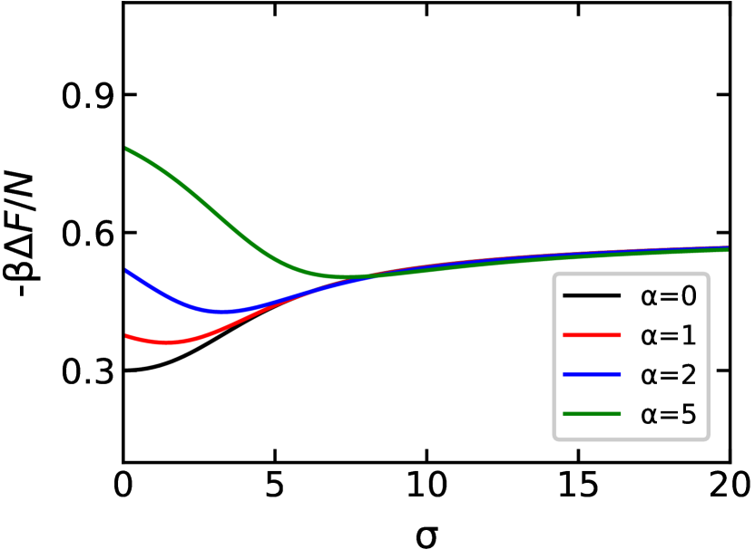
Figure 4: The contribution of dipole-dipole interactions $\Delta F$ for the perpendicular configuration as a function of the anisotropy parameter $\sigma$ for the system with $\lambda_{e}=0.5$ and different values of $\alpha$ = 0, 1, 2 and 5.

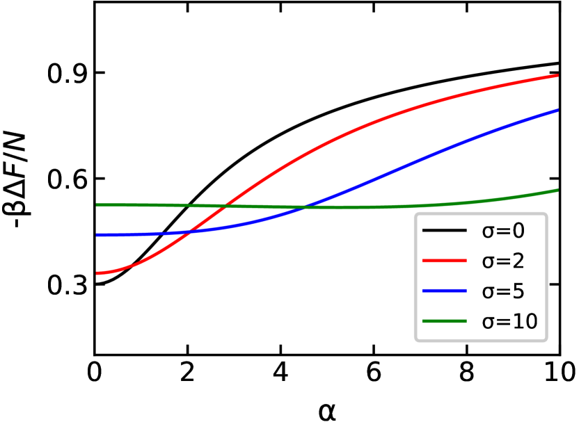
Figure 5: The contribution of dipole-dipole interactions $\Delta F$ for the perpendicular configuration as a function of the Langevin parameter $\alpha$ for the system with $\lambda_{e}=0.5$ and different values of $\sigma$ = 0, 2, 5 and 10.

II.5 Simulation

In order to check the accuracy of the new theory and discover its applicability, its predictions were thoroughly tested against computer simulation data. Monte Carlo (MC) simulations were carried out in a canonical (NVT) ensemble for $N=512$ dipolar hard spheres embedded in the lattice nodes. The model configuration was generated inside a cubic box, to which 3D periodic boundary conditions were applied. To vanish all the demagnetization effects, the Ewald summation with conducting boundary conditions was used for computing the long-range dipole-dipole interactions between magnetic nanoparticles. It was assumed that the external magnetic field was directed along the $Oz$ axis. The easy axes were the unit vectors parallel to (i) the laboratory Oz axis in the parallel configuration and (ii) the laboratory Ox axis in the perpendicular configuration. To overcome the anisotropy barrier for high values of $\sigma$, there were two equiprobable types of rotational move: ordinary random displacement and the flip move $\textbf{m}\rightarrow-\textbf{m}$ Elfimova et al. (2019). Typical run lengths consisted of $10^{6}$ attempted rotations per nanoparticle after equilibration. Estimates of statistical errors were calculated using the blocking procedure described in Allen and Tildesley (1987). In all cases, the obtained values of statistical errors do not exceed the size of symbols used for the simulation data.

The Helmholtz free energy can not be measured by the numerical method directly, so its derivatives (the scalar magnetization and the initial magnetic susceptibility) were used to investigate the validity of the new theory. For both the parallel and perpendicular configurations, fractional magnetization was computed in the simulation as

$$M=\frac{1}{N}\left\langle\sum_{i=1}^{N}\cos\omega_{i}\right\rangle_{t},$$ (43)

where $\langle\ldots\rangle_{t}$ means the average over simulation time. The initial magnetic susceptibility was calculated at $\alpha=0$ in the $z$ direction only:

$$\chi=\chi_{L}\Bigg{\langle}\left(\sum_{i=1}^{N}\cos\omega_{i}\right)^{2}\Bigg{\rangle}_{t}\frac{3}{N},$$ (44)

where the Langevin susceptibility $\chi_{L}$ can be expressed via parameter $\lambda_{e}$ using the relation $\rho=1/a^{3}$ for the simple cubic lattice

$$\chi_{L}=\frac{4\pi\mu_{0}\rho m^{2}}{3k_{B}T}=\frac{4\pi}{3}\lambda_{e}.$$ (45)

To check the simulation algorithm with high values of the anisotropy parameter, an ideal system of superparamagnetic nanoparticles was modeled where interparticle interaction was turned off. In this case, the exact theoretical results are known:

$$M_{\textrm{\scriptsize{id}}} = -\frac{\partial}{\partial\alpha}\left(\frac{\beta F_{\textrm{\scriptsize{id}}}}{N}\right),$$ (46)

$$\chi_{\textrm{\scriptsize{id}}} = -\frac{1}{V}\frac{\partial^{2}F_{\textrm{\scriptsize{id}}}}{\partial H^{2}}\Bigg{|}_{H=0},$$ (47)

where $F_{\textrm{\scriptsize{id}}}$ is defined by (32) for the parallel configuration and (38) for the perpendicular configuration. In Figs. 6 and 7, one can find the excellent agreement between obtained simulation data and ideal approximations (46) and (47) for both magnetization and the initial magnetic susceptibility.

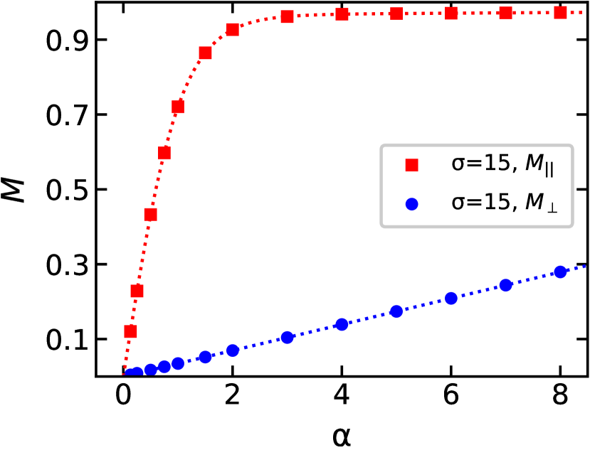
Figure 6: The static magnetization as a function of the Langevin parameter $\alpha$ for a system with $\sigma=15$ in the absence of interparticle interactions. Dashed lines correspond to the ideal approximation (46). The symbols are from Monte-Carlo simulations. The results are shown for the parallel (red squares and line) and perpendicular (blue circles and line) configurations.

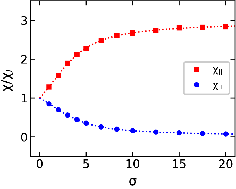
Figure 7: The initial magnetic susceptibility $\chi$ divided by the Langevin susceptibility $\chi_{L}$ as a function of the anisotropy parameter $\sigma$ for a system without interparticle interactions. Dashed lines correspond to the ideal approximation (47). The symbols are from Monte-Carlo simulations. The results are shown for the parallel (red squares and lines) and perpendicular (blue circles and lines) configurations.

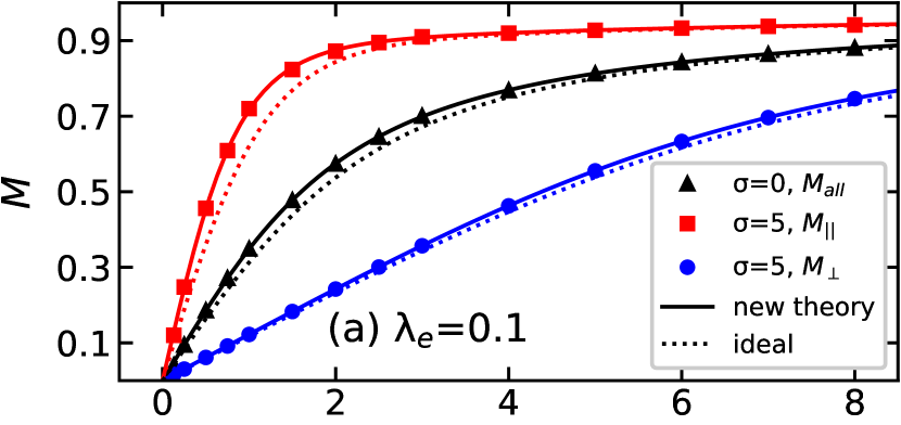
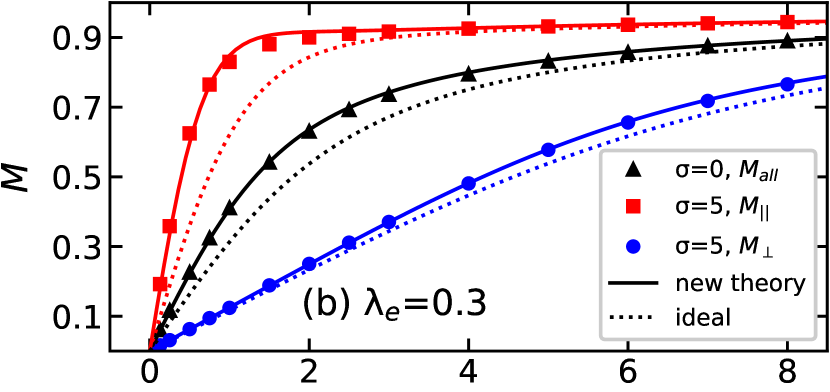
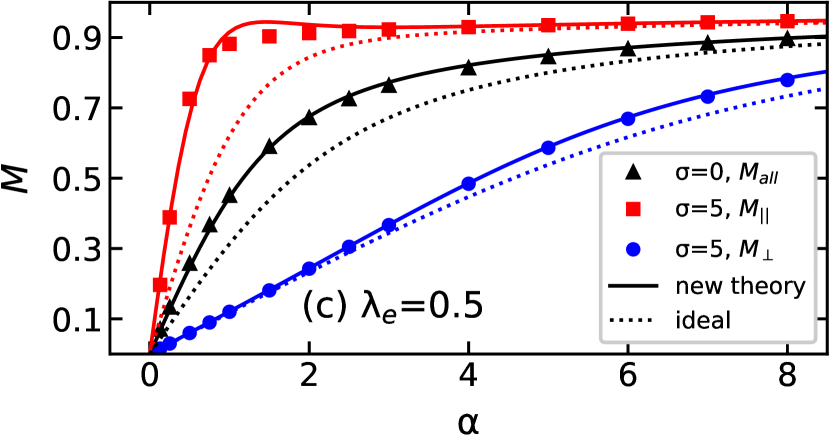
Figure 8: The static magnetization as a function of the Langevin parameter $\alpha$ for systems with (a) $\lambda_{e}=0.1$, (b) 0.3 and (c) 0.5. The solid lines correspond to the new theories for $M_{||}$ and $M_{\perp}$, the dashed lines are the ideal approximation (46). The symbols are from Monte-Carlo simulations. The results are shown for the parallel (red squares and lines) and the perpendicular (blue circles and lines) configurations with $\sigma=5$ and for the system with $\sigma=0$ (black triangles and lines).

III Results

The analytical expression of the Helmholtz free energy allows us to obtain predictions for the various magnetic and thermodynamic properties of the system. So, the scalar magnetization is defined by

$$M = M_{\textrm{\scriptsize{id}}}-\frac{\partial}{\partial\alpha}\left(\frac{\beta\Delta F}{N}\right),$$ (48)

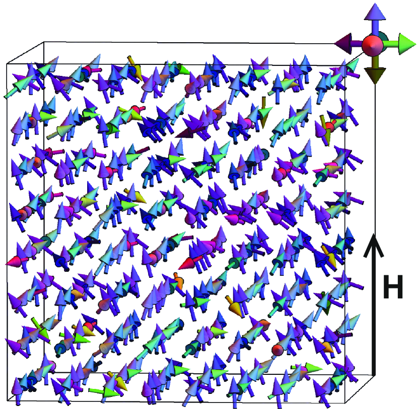
(a) $\alpha=1$, $\sigma=0$, $M_{all}=0.45$

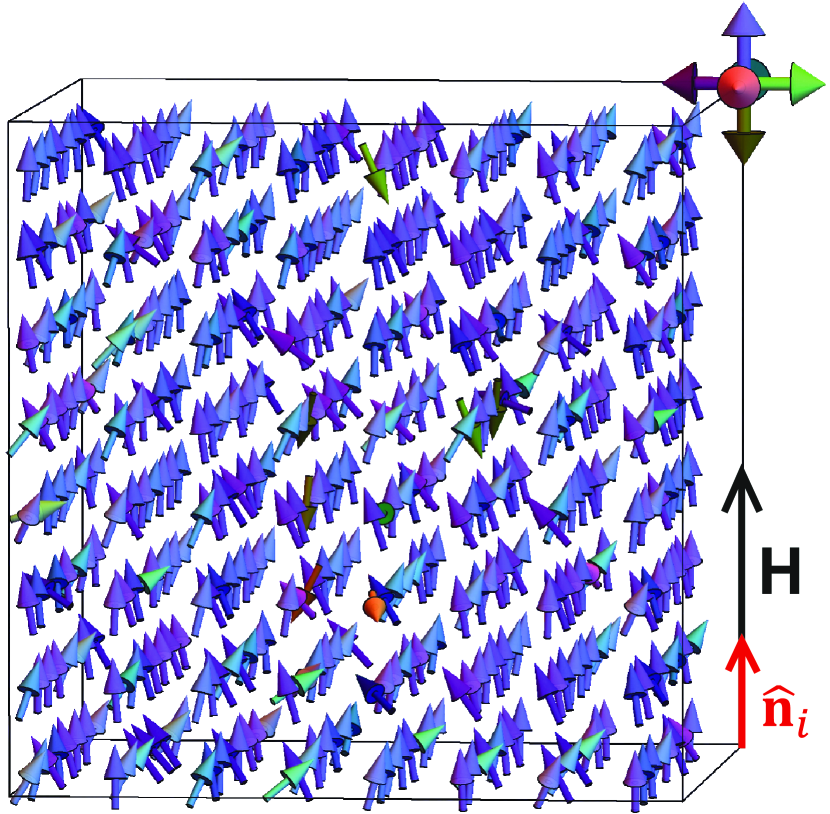
(b) $\alpha=1$, $\sigma=5$, $M_{\|}=0.88$

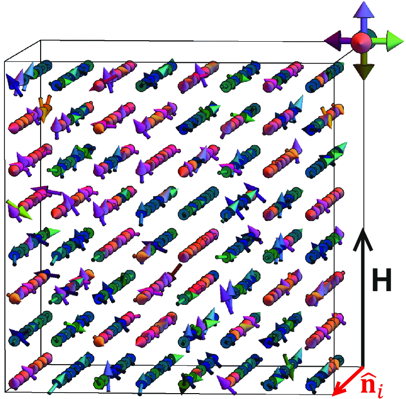
(c) $\alpha=1$, $\sigma=5$, $M_{\perp}=0.12$

Figure 9: Simulation snapshots of a model system with $\lambda_{e}=0.5$ and $\alpha=1$. The results are shown for (a) $\sigma=0$, (b) parallel configurations with $\sigma=5$ and (c) perpendicular configurations with $\sigma=~{}5$. Different arrow colors correspond to different orientations of the magnetic moments.

where $\Delta F$ can be found in (37) for the parallel configuration and (42) for the perpendicular configuration. The second term takes into account the interparticle dipole-dipole interactions in the model system. Three systems were considered: $\lambda_{e}=0.1$, 0.3 and 0.5. The Langevin susceptibilities for these systems are equal to $\chi_{L}=0.42$, 1.26 and 2.1, respectively. In Fig. 8, the theoretical static magnetization curves are compared with the MC simulation data. For $\sigma=0$ (black curves), the theoretical predictions for both the parallel and perpendicular configurations coincide with each other, as was expected. In this case, the excellent agreement of the new theory (solid lines) with the simulation data for all considered systems should be noted, whereas the ideal approximation (dashed lines) works well only for a system with a weak interactions ($\lambda_{e}=0.1$). The same can be said about the perpendicular configuration with $\sigma=5$ (blue curves). The magnetization of the parallel configuration with $\sigma=5$ increases rapidly as the magnetic field intensity increases, and the dipole-dipole interaction effect is more pronounced in this case. However, for $\sigma=5$ and $\lambda_{e}=0.5$, a small deviation between the new theoretical formula (48) and the simulation data is observed in the range of magnetic field $1\leq\alpha\leq 2$.

The typical behavior of the magnetization can be described as follows: an increase in $\sigma$ leads to an increase in the magnetization in the parallel case and a decrease in the perpendicular configuration. This fact is clearly illustrated in Fig. 9, where simulation snapshots are given for the model system with $\lambda_{e}=0.5$ and $\alpha=1$. Fig. 9 (a) corresponds to when $\sigma=0$ and scalar magnetization is equal to $M=0.45$. The presence of an easy axis with $\sigma=5$ along the external magnetic field almost doubles the scalar magnetization, as shown in Fig. 9 (b). The perpendicular configuration with $\sigma=5$ is given in Fig. 9 (c), where the system’s magnetic response to the external magnetic field is very weak. In this case, the magnetic moments formed chains in the direction of the easy axis so that scalar magnetization in the direction of $\hat{\textbf{n}}_{i}$ is equal to zero, although a pronounced regular structure in the magnetic moments of all the system’s nanoparticles is not yet observed.

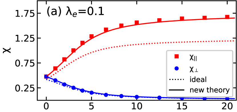
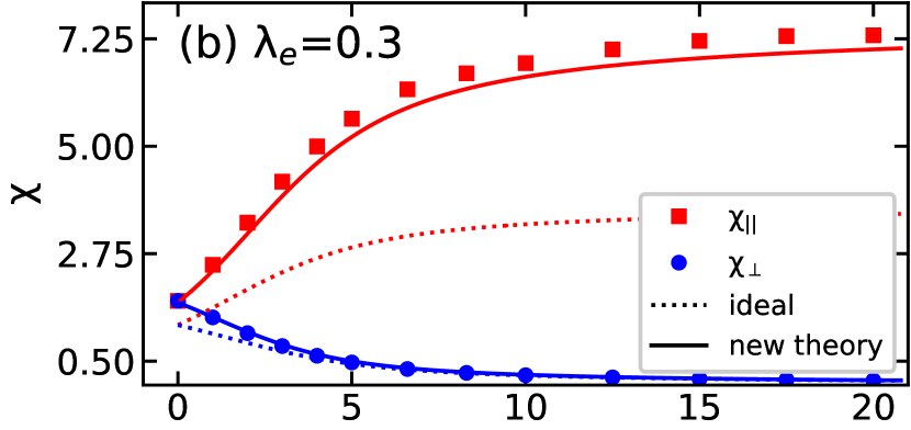
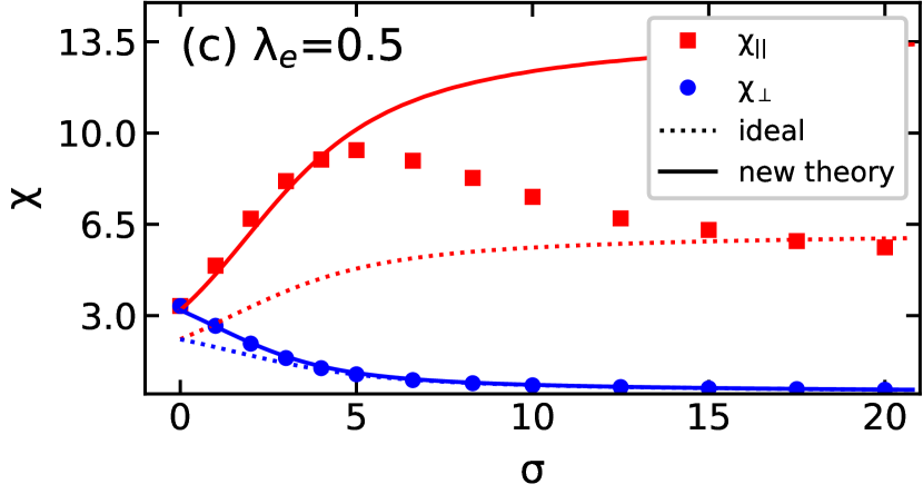
Figure 10: The initial magnetic susceptibility $\chi$ as a function of anisotropy parameter $\sigma$ for systems with (a) $\lambda_{e}=0.1$, (b) 0.3 and (c) 0.5. The solid lines correspond to new theories for $\chi_{||}$ and $\chi_{\perp}$, the dashed lines are the ideal approximation (47). The symbols are from Monte-Carlo simulations. The results are shown for the parallel (red squares and lines) and perpendicular (blue circles and lines) configurations.

The initial slope of the magnetization curve is characterized by the initial magnetic susceptibility, which can be determined via the Helmholtz free energy as

$$\chi=\chi_{\textrm{\scriptsize{id}}}-\frac{1}{V}\frac{\partial^{2}\Delta F}{\partial H^{2}}\Bigg{|}_{H=0}.$$ (49)

A comparison between the theoretical predictions of $\chi$ and the MC results is given in Fig. 10. The results are shown for both the parallel and perpendicular configurations. As for ideal approximations (47), there is a significant discrepancy between the dashed curves and the simulation data in all the considered systems, but especially for the parallel configuration. Even for a weakly interacting system with $\lambda_{e}=0.1$, see Fig. 10 (a), the difference between the susceptibilities of the non-interacting (red dashed line) and interacting nanoparticles (red solid line) for the parallel configuration is surprisingly large. Interactions lead a rapid growth in susceptibility, and the new theory (49) allows for an accurate description of this behavior in $\chi_{\|}$. One can note a strong agreement between the new theory (solid lines) and the MC data (symbols) for both the parallel and perpendicular configurations at $\lambda_{e}=0.1$. As $\lambda_{e}$ increases up to 0.3 in Fig. 10 (b), a small deviation between the new theory (49) and the simulation data appears in the parallel configuration (red color), while for the perpendicular configuration (blue color), the agreement of theoretical and numerical results remains strong. The MC results for the parallel configuration at $\lambda_{e}=0.5$ (Fig. 10 (c)) demonstrate an unexpected effect: the non-monotonic behavior of susceptibility as $\sigma$ increases. Note that the maximum achievable susceptibility value in this case is $\chi_{\|}\simeq 9$ at $\sigma\simeq 5$.

The potential reason for this behavior is that the total magnetic moment of the system decreases due to the appearance of magnetically compensated structures. This suggestion can be confirmed from a visual examination of the simulation snapshots given in Fig. 11. The viewing angle on the system is changed to provide more clarity: the blue vectors correspond to the direction of the $Oz$ axis. All systems have a high value of the anisotropy parameter $\sigma=20$, which leads to a rigid alignment of the magnetic moments along the easy axes. For the system with $\lambda_{e}=0.3$ (Fig. 11 (a)), there are no regular structures in the direction of the magnetic moments: the snapshot contains many possible alignment variations of the magnetic moments in inner chains along the easy axis. Fig. 11 (b) shows that for the system with $\lambda_{e}=0.5$, a pronounced arrangement of the magnetic moments in chains along the easy axes is present: these are directed mainly in one direction within a single chain. Increasing the intensity of dipole interactions up to $\lambda_{e}=1$ (Fig. 11 (c)), we note an additional tendency in the antiparallel alignment of chains along the easy axes, which leads to a further decrease in the system susceptibility. This case requires some discussion. The plane perpendicular to $\hat{\bm{n}_{i}}$ in Fig. 11 (c) has a clear checkerboard pattern, since there are four antiparallel neighbors for each chain parallel to $\hat{\bm{n}_{i}}$. For a single nanoparticle, it is possible to conclude the following about its six nearest neighbors: two form the most conducive orientation “head-to-tail”; the next four have the second-most advantageous orientation “side-by-side”. The magnetic response of such a system is very weak and needs a strong applied magnetic field to obtain the magneto-active material.

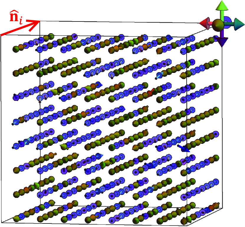
(a) $\lambda_{e}=0.3$, $\chi_{\|}=7.32$

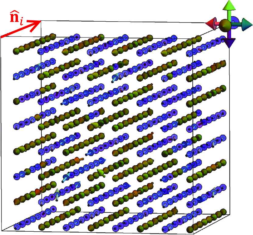
(b) $\lambda_{e}=0.5$, $\chi_{\|}=5.62$

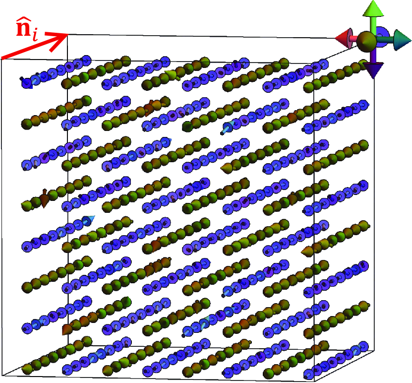
(c) $\lambda_{e}=1.0$, $\chi_{\|}=0.16$

Figure 11: Simulation snapshots of the model system with $\alpha=0$ and $\sigma=20$. Results are shown for parallel configurations with (a) $\lambda_{e}=0.3$, (b) $\lambda_{e}=0.5$ and (c) $\lambda_{e}=1.0$. Different arrow colors correspond to different orientations of magnetic moments. The viewing angle on the system is changed to more clarity.

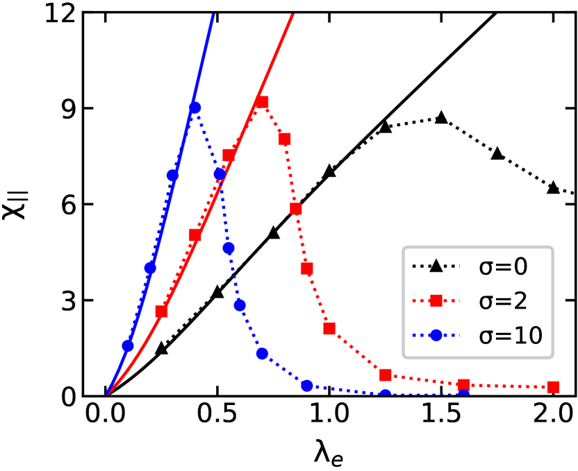
Figure 12: The initial magnetic susceptibility $\chi_{||}$ as a function of parameter $\lambda_{e}$ for parallel configuration. The solid lines correspond to the new theory for $\chi_{||}$. The symbols are from the Monte-Carlo simulations. The results are shown for systems with $\sigma=0$ (black triangles and lines), $\sigma=2$ (red squares and lines) and $\sigma=10$ (blue circles and lines).

From Fig. 11, one can conclude that the dependency of $\chi_{\|}$ as a function of $\lambda_{e}$ at a fixed value of $\sigma$ is also non-monotonic. This fact was observed in Ref. Solovyova et al. (2020) at $\sigma=0$: the Molecular Dynamic simulation results are denoted in Fig. 12 by the black symbols with the dashed black curve. The excellent agreement between the new theory (49) and the simulation data up to $\lambda_{e}\sim 1.25$ should be noted, when there are no structural transformations in the magnetic systems. A further increase in interaction intensity leads to a decrease in susceptibility, the reason for which is the particular behavior of the dipole ordering: almost all the magnetic moments are aligned in long antiparallel chains along the direction of the easy axis. During the current investigation, the dependency of $\chi_{\|}$ as a function of $\lambda_{e}$ was calculated for systems with an easy axis, the anisotropy parameters of which had the values $\sigma=2$ and 10. The obtained MC results are denoted in Fig. 12 as red symbols with a dashed red curve and blue symbols with a dashed blue curve, respectively. The increasing of $\sigma$ causes a shift in the susceptibility maximum to the left. The value of this shift from $\sigma=0$ to 2 is greater than from $\sigma=2$ to 10. It should also be stressed that susceptibility begins to decline when the value $\chi_{\|}\simeq 9$ is reached, regardless of the value of the anisotropy parameter $\sigma$. This is consistent with the results from Fig. 10 (c): susceptibility increases as $\sigma$ increases up to the value of $\chi_{\|}\simeq 9$ and then decreases further. This fact allows us to conclude that the model system can demonstrate the maximum value of susceptibility in the parallel configuration $\chi_{\|}\simeq 9$, and that this is an inherent property of the considered nanoparticle placement on the nodes of the simple cubic lattice. It should be emphasized that in a system of interacting immobilized superparamagnetic nanoparticles located randomly, the pronounced regular structuring of the magnetic moments is not observed with the parameters under consideration Elfimova et al. (2019).

The new theory is able to predict the magnetic properties of the model system over a range of parameters $\lambda_{e}$ and $\sigma$, for which the susceptibility value is $\chi_{\|}\leq 9$ and there is no regular structuring of nanoparticle magnetic moments. To clarify this range, it is possible to plot a phase diagram using the MC data from Fig. 10:

• at $\lambda_{e}=0.3$ new theory works well up to $\sigma=20$;

• at $\lambda_{e}=0.5$ new theory works well up to $\sigma=5$;

and from Fig. 12:

• at $\sigma=0$ new theory works well up to $\lambda_{e}=1.25$;

• at $\sigma=2$ new theory works well up to $\lambda_{e}=0.7$;

• at $\sigma=10$ new theory works well up to $\lambda_{e}=0.4$.

The range of the applicability of the new theory is denoted as the grey area in Fig. 13. The area above the dashed line indicates an ordered state with the presence of ferromagnetic chains arranged antiferromagnetically in zero fields, which leads to a decrease in susceptibility. The antiferromagnetic ordering of the magnetic moments was also discovered in a study of the ground state of dipoles embedded in simple cubic lattice nodes in the absence of an external magnetic field Kretschmer and Binder (1979).

The deviation of new theory from the results of computer modeling in Figs. 10 (c), 12 is connected with the consideration of only the pair correlations in the system and the truncation of the Helmholtz free energy expansions (37), (42) up to the third power of the effective dipolar coupling constant. To expand the given scope of the new theory, one can try to increase the number of terms in the virial series. However, when applying the virial expansion method, it is difficult to construct a theoretical approach valid for systems with a strong dipolar regime. In this case, an alternative method can be used, for instance Budkov and Kiselev (2018); Budkov and Kolesnikov (2016).

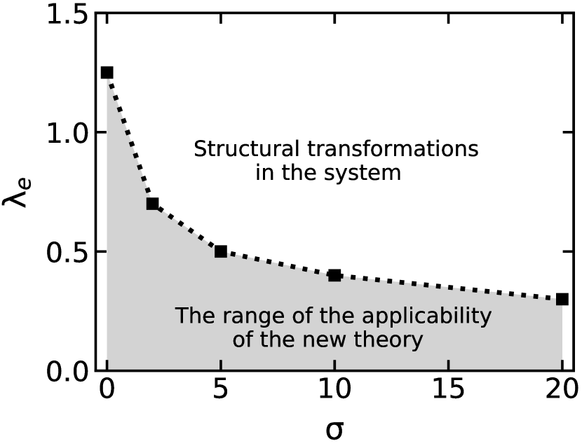
Figure 13: The phase diagram of the uniaxial superparamagnetic nanoparticles embedded in a simple cubic lattice. The grey area corresponds to the state of a system without the regular structuring of the particle magnetic moments, where the new theory (49), (37), (42) is able to describe the magnetic properties of the model.

IV Conclusion

The static magnetic response of a simple cubic lattice of interacting superparamagnetic nanoparticles has been studied via theory and simulation. The potential energy of the system includes one-particle dipole-easy axis interaction, one-particle dipole-field interaction, and long-range interparticle dipole-dipole interactions. Two orientational distributions of the easy axis in the system have been considered: aligned parallel and perpendicular to the direction of an external magnetic field. For both cases, a theoretical expression for the Helmholtz free energy in logarithmic form has been derived considering pairwise dipole-dipole interactions from the rigorous methods of statistical physics. Using the obtained formula for the Helmholtz free energy, the magnetic properties have been investigated over a broad range of parameters. The theoretical predictions have been critically compared with MC simulation data.

For the parallel configuration, the magnetic moments are preferably aligned along the direction of the field, which strongly enhances magnetization. For the perpendicular configuration, the magnetic moments are held by the easy axes perpendicular to the field: magnetization decreases as the anisotropy parameter $\sigma$ increases. In both cases, interparticle dipole-dipole interactions lead to an increase in magnetization, but this enhancement is much greater for the parallel configuration. The ideal approach is not capable of describing the simulation data adequately, whereas the theory examined in this paper (which takes into account interparticle interactions) is much more efficient.

The susceptibility curves from the MC simulations have demonstrated several interesting new results. Firstly, non-monotonic behavior of $\chi_{\|}$ has been observed as the anisotropy parameter or the dipole-dipole interaction intensity increase. For a system of interacting immobilized superparamagnetic nanoparticles located randomly, the initial magnetic susceptibility increases monotonically as the anisotropy parameter or the dipole-dipole interaction intensity increase Elfimova et al. (2019). Secondly, for any set of intrinsic parameters, the maximum achievable value of $\chi_{\|}$ is equal to $\simeq 9$. This allows us to conclude that the system under consideration undergoes a phase transition in the ordering of magnetic moments. The phase diagram of the orientational state of the magnetic moments was plotted along the $\lambda_{e}$ – $\sigma$ axes, which shows the region with regular orientational structuring of the magnetic moments and the region lacking any orientational structures. The theoretic susceptibility curves are in strong agreement with the MC data only for parameters that correspond to the system without regular structuring of the magnetic moments. The obtained results are important for the development of functional magnetic materials with controlled properties.

Appendix A: Parallel Configuration

For the parallel configuration, the results of averaging the coefficients $b_{1}$, $b_{2}$, $b_{3}$ over the magnetic moment orientations can be written as follows:

$$b_{1} = 2Q_{1}^{2}(\alpha,\sigma)\gamma_{12},$$ (A.1)

$$b_{2} = \frac{36}{35}Q_{2}^{2}(\alpha,\sigma)\gamma_{24}$$ (A.2)

$$+ \frac{2}{3}Q_{2}(\alpha,\sigma)\left(1-\frac{Q_{2}(\alpha,\sigma)}{7}\right)\gamma_{22}$$

$$+ \frac{1}{3}\left(1+\frac{Q_{2}^{2}(\alpha,\sigma)}{5}\right)\gamma_{20},$$

$$b_{3} = \frac{6}{77}\big{(}3Q_{1}(\alpha,\sigma)-5Q_{3}(\alpha,\sigma)\big{)}^{2}\gamma_{36}$$ (A.3)

$$+ \frac{18}{11}\bigg{(}\frac{4Q_{1}(\alpha,\sigma)Q_{3}(\alpha,\sigma)}{5}-\frac{3Q_{1}^{2}(\alpha,\sigma)}{7}$$

$$- \frac{Q_{3}^{2}(\alpha,\sigma)}{7}\bigg{)}\gamma_{34}+\frac{1}{7}\left(3Q_{1}^{2}(\alpha,\sigma)+Q_{3}^{2}(\alpha,\sigma)\right)\gamma_{32}$$

$$+ \frac{1}{42}\bigg{(}\frac{6Q_{1}(\alpha,\sigma)Q_{3}(\alpha,\sigma)}{5}+3Q_{1}^{2}(\alpha,\sigma)$$

$$- Q_{3}^{2}(\alpha,\sigma)\bigg{)}\gamma_{30},$$

where several functions have been introduced as

$$Q_{1}(\alpha,\sigma) = \frac{1}{2Q_{0}(\alpha,\sigma)}\int\limits_{-1}^{1}\exp\left(\alpha t+\sigma t^{2}\right)t\ dt,\ \ \$$ (A.4)

$$Q_{1}(\alpha,0) = L(\alpha),$$

$$L(\alpha) = \coth\alpha-\frac{1}{\alpha},$$

$$Q_{2}(\alpha,\sigma) = \frac{3}{4Q_{0}(\alpha,\sigma)}\int\limits_{-1}^{1}\exp\left(\alpha t+\sigma t^{2}\right)t^{2}\ dt$$ (A.5)

$$- \frac{1}{2},\ \ \ \ \ \ \$$

$$Q_{2}(\alpha,0) = L_{3}(\alpha),$$

$$L_{3}(\alpha) = 1-3\frac{L(\alpha)}{\alpha},$$

$$Q_{3}(\alpha,\sigma) = \frac{1}{2Q_{0}(\alpha,\sigma)}\int\limits_{-1}^{1}\exp\left(\alpha t+\sigma t^{2}\right)t^{3}\ dt,\ \ \ \ \ \$$ (A.6)

$$Q_{3}(\alpha,0) = L(\alpha)-\frac{2}{\alpha}L_{3}(\alpha).$$

The numbers $\gamma_{pq}$ involve the sum of position-dependent expressions over the nodes of the cubic lattice, limited by cylinder size:

$$\gamma_{pq} = \sum\limits_{j=2}^{N}\frac{1}{\tilde{r}_{1j}^{3p}}P_{q}\left(\frac{\tilde{z}_{1j}}{\tilde{r}_{1j}}\right),$$ (A.7)

This definition introduces the dimensionless interparticle separation vector $\tilde{\textbf{r}}_{1j}=\textbf{r}_{1j}/a$, where $\tilde{z}_{1j}$ is the z-component of vector $\tilde{\textbf{r}}_{1j}$ in the laboratory coordinate system shown in Fig. 1 (a). $P_{q}$ $(q=0,2,4,6)$ in (A.7) denote Legendre polynomials. It is assumed that the nanoparticle 1 is fixed at the origin of the laboratory frame. All the other nodes of the simple cubic lattice except $(\tilde{x}_{1},\tilde{y}_{1},\tilde{z}_{1})\equiv(0,0,0)$, can be occupied by nanoparticle j

$$-R\leqslant \tilde{x}_{j}\leqslant R,$$

$$-R\leqslant \tilde{y}_{j}\leqslant R,$$

$$-hR\leqslant \tilde{z}_{j}\leqslant hR,$$ (A.8)

$$\left(\tilde{x}_{j}\right)^{2}+ \left(\tilde{y}_{j}\right)^{2} \leqslant R^{2},$$

$$\left(\tilde{x}_{j}\right)^{2}+ \left(\tilde{y}_{j}\right)^{2} +\left(\tilde{z}_{j}\right)^{2}>0.$$

The cylinder is limited by the dimensionless radius R and the height $2h$. The results for $\gamma_{pq}$ obtained for model system with $N\simeq 25\times 10^{6}$ ferroparticles are $\gamma_{12}=2.0944$, $\gamma_{24}=3.2257$, $\gamma_{22}=\gamma_{32}=0$, $\gamma_{20}=8.4016$, $\gamma_{36}=0.6553$, $\gamma_{34}=3.4081$, $\gamma_{30}=6.6289$.

Appendix B: Perpendicular Configuration

For the perpendicular configuration, the results of averaging the coefficients $b_{1}$, $b_{2}$, $b_{3}$ over magnetic moment orientations can be written as follows:

$$b_{1} = 2R_{1}^{2}(\alpha,\sigma)\epsilon_{1},$$ (B.1)

$$b_{2} = \left(R_{2}^{2}(\alpha,\sigma)+3R_{3}^{2}(\alpha,\sigma)-2R_{3}(\alpha,\sigma)+1\right)\epsilon_{2}$$ (B.2)

$$+ \frac{9}{4}\left(2R_{3}(\alpha,\sigma)-3R_{3}^{2}(\alpha,\sigma)-R_{2}^{2}(\alpha,\sigma)+1\right)\epsilon_{3}$$

$$+ \frac{9}{4}\epsilon_{3},\ \ \ \ \ \ \$$

$$b_{3} = \frac{4}{3}R_{5}^{2}(\alpha,\sigma)\epsilon_{4}$$ (B.3)

$$+ 4\left[(R_{4}(\alpha,\sigma)-R_{5}(\alpha,\sigma))^{2}+R_{6}^{2}(\alpha,\sigma)\right]\epsilon_{5}$$

$$+ 18\big{[}R_{4}^{2}(\alpha,\sigma)+R_{6}^{2}(\alpha,\sigma)+R_{5}(\alpha,\sigma)R_{6}(\alpha,\sigma)$$

$$- R_{4}(\alpha,\sigma)R_{5}(\alpha,\sigma)\big{]}\epsilon_{6}$$

$$+ 9(R_{4}(\alpha,\sigma)-R_{5}(\alpha,\sigma))R_{6}(\alpha,\sigma)\epsilon_{7},$$

where additional functions have been introduced as

$$R_{1}(\alpha,\sigma) = \int\limits_{0}^{1}\exp\left(\sigma t^{2}\right)I_{0}(\alpha\sqrt{1-t^{2}})\sqrt{1-t^{2}}dt$$ (B.4)

$$\times \left[R_{0}(\alpha,\sigma)\right]^{-1},$$

$$R_{1}(\alpha,0) = L(\alpha),$$

$$R_{2}(\alpha,\sigma) = \int\limits_{0}^{1}\exp\left(\sigma t^{2}\right)I_{2}(\alpha\sqrt{1-t^{2}})\left(1-t^{2}\right)dt$$ (B.5)

$$\times \left[R_{0}(\alpha,\sigma)\right]^{-1},$$

$$R_{2}(\alpha,0) = L_{3}(\alpha),$$

$$R_{3}(\alpha,\sigma) = \int\limits_{0}^{1}\exp\left(\sigma t^{2}\right)I_{0}(\alpha\sqrt{1-t^{2}})t^{2}dt$$ (B.6)

$$\times \left[R_{0}(\alpha,\sigma)\right]^{-1},$$

$$R_{3}(\alpha,0) = \frac{L(\alpha)}{\alpha},$$

$$R_{4}(\alpha,\sigma) = \int\limits_{0}^{1}\exp\left(\sigma t^{2}\right)I_{1}(\alpha\sqrt{1-t^{2}})\sqrt{1-t^{2}}^{3}dt$$ (B.7)

$$\times \left[R_{0}(\alpha,\sigma)\right]^{-1},$$

$$R_{4}(\alpha,0) = L(\alpha)-\frac{L_{3}(\alpha)}{\alpha},$$

$$R_{5}(\alpha,\sigma) = \int\limits_{0}^{1}\exp\left(\sigma t^{2}\right)I_{3}(\alpha\sqrt{1-t^{2}})\sqrt{1-t^{2}}^{3}dt$$ (B.8)

$$\times \left[R_{0}(\alpha,\sigma)\right]^{-1},$$

$$R_{5}(\alpha,0) = L(\alpha)-2\frac{L_{3}(\alpha)}{\alpha},$$

$$R_{6}(\alpha,\sigma) = \int\limits_{0}^{1}\exp\left(\sigma t^{2}\right)I_{1}(\alpha\sqrt{1-t^{2}})\sqrt{1-t^{2}}t^{2}dt$$ (B.9)

$$\times \left[R_{0}(\alpha,\sigma)\right]^{-1},$$

$$R_{6}(\alpha,0) = \frac{L_{3}(\alpha)}{\alpha}.$$

Here, $I_{k}(x)$ is the modified Bessel function of k order, the numbers $\epsilon_{k}$ involve the sum of position-dependent expressions over the nodes of the cubic lattice, limited by cylinder size:

$$\epsilon_{1} = \sum\limits_{j=2}^{N}\frac{1}{\tilde{r}_{1j}^{3}}P_{2}\left(\frac{\tilde{x}_{1j}}{\tilde{r}_{1j}}\right)\simeq 2.0944,$$ (B.10)

$$\epsilon_{2} = \sum\limits_{j=2}^{N}\frac{1}{\tilde{r}_{1j}^{6}}P_{2}^{2}\left(\frac{\tilde{x}_{1j}}{\tilde{r}_{1j}}\right)\simeq 3.3393,$$ (B.11)

$$\epsilon_{3} = \sum\limits_{j=2}^{N}\frac{\tilde{x}_{1j}^{2}\tilde{z}_{1j}^{2}}{\tilde{r}_{1j}^{10}}\simeq 0.1915,$$ (B.12)

$$\epsilon_{4} = \sum\limits_{j=2}^{N}\frac{1}{\tilde{r}_{1j}^{9}}P_{2}^{3}\left(\frac{\tilde{x}_{1j}}{\tilde{r}_{1j}}\right)\simeq 1.4880,$$ (B.13)

$$\epsilon_{5} = \sum\limits_{j=2}^{N}\frac{1}{\tilde{r}_{1j}^{9}}P_{2}\left(\frac{\tilde{x}_{1j}}{\tilde{r}_{1j}}\right)P_{2}^{2}\left(\frac{\tilde{z}_{1j}}{\tilde{r}_{1j}}\right)$$ (B.14)

$$\simeq -0.7440,$$

$$\epsilon_{6} = \sum\limits_{j=2}^{N}\frac{\tilde{x}_{1j}^{2}\tilde{z}_{1j}^{2}}{\tilde{r}_{1j}^{13}}P_{2}\left(\frac{\tilde{z}_{1j}}{\tilde{r}_{1j}}\right)\simeq 0.0114,$$ (B.15)

$$\epsilon_{7} = \sum\limits_{j=2}^{N}\frac{\tilde{y}_{1j}^{2}\tilde{z}_{1j}^{2}(8\tilde{x}_{1j}^{2}-\tilde{y}_{1j}^{2}-\tilde{z}_{1j}^{2})}{\tilde{r}_{1j}^{15}}$$ (B.16)

$$\simeq -0.0318.\ \ \ \$$

References

- Kuznetsova et al. (2019) I.E. Kuznetsova, V.V. Kolesov, A.S. Fionov, E.Y. Kramarenko, G.V. Stepanov, M.G. Mikheev, E. Verona, and I. Solodov, “Magnetoactive elastomers with controllable radio-absorbing properties,” Materials Today Communications 21, 100610 (2019).
- Borin et al. (2019) D. Borin, G. Stepanov, and E. Dohmen, “Hybrid magnetoactive elastomer with a soft matrix and mixed powder,” Archive of Applied Mechanics 89, 105–117 (2019).
- Filipcsei et al. (2007) G. Filipcsei, I. Csetneki, A. Szilágyi, and M. Zrínyi, “Magnetic field-responsive smart polymer composites,” Advances in Polymer Science 206, 137–189 (2007).
- Blyakhman et al. (2019) F.A. Blyakhman, E.B. Makarova, F.A. Fadeyev, D.V. Lugovets, A.P. Safronov, P.A. Shabadrov, T.F. Shklyar, G.Y. Melnikov, I. Orue, and G.V. Kurlyandskaya, “The contribution of magnetic nanoparticles to ferrogel biophysical properties,” Nanomaterials 9, 232 (2019).
- Dutz and Hergt (2013) S. Dutz and R. Hergt, “Magnetic nanoparticle heating and heat transfer on a microscale: Basic principles, realities and physical limitations of hyperthermia for tumour therapy,” International Journal of Hyperthermia 29, 790–800 (2013).
- Ortega and Pankhurst (2013) D. Ortega and Q. A. Pankhurst, “Magnetic hyperthermia,” Nanoscience 1, 60–88 (2013).
- Zubarev (2018) A.Yu. Zubarev, “Magnetic hyperthermia in a system of ferromagnetic particles, frozen in a carrier medium: Effect of interparticle interactions,” Physical Review E 98, 032610 (2018).
- Zubarev (2019) A.Yu. Zubarev, “Magnetic hyperthermia in a system of immobilized magnetically interacting particles,” Physical Review E 99, 062609 (2019).
- Zhang et al. (2017) W. Zhang, X. Zuo, Y. Niu, C. Wu, S. Wang, S. Guan, and S.R.P. Silva, “Novel nanoparticles with cr3+ substituted ferrite for self-regulating temperature hyperthermia,” Nanoscale 9, 13929–13937 (2017).
- Piehler et al. (2020) S. Piehler, H. Dähring, J. Grandke, J. Göring, P. Couleaud, A. Aires, A.L. Cortajarena, J. Courty, A. Latorre, A. Somoza, U. Teichgräber, and I. Hilger, “Iron oxide nanoparticles as carriers for dox and magnetic hyperthermia after intratumoral application into breast cancer in mice: impact and future perspectives,” Nanomaterials 10, 1016 (2020).
- Brero et al. (2020) F. Brero, M. Albino, A. Antoccia, P. Arosio, M. Avolio, F. Berardinelli, D. Bettega, P. Calzolari, M. Ciocca, M. Corti, A. Facoetti, S. Gallo, F. Groppi, A. Guerrini, C. Innocenti, C. Lenardi, S. Locarno, S. Manenti, R. Marchesini, M. Mariani, F. Orsini, E. Pignoli, C. Sangregorio, I. Veronese, and A. Lascialfari, “Hadron therapy, magnetic nanoparticles and hyperthermia: A promising combined tool for pancreatic cancer treatment,” Nanomaterials 10, 1919 (2020).
- Raikher and Shliomis (1974) Yu.L. Raikher and M.I. Shliomis, “Theory of dispersion of the magnetic susceptibility of fine ferromagnetic particles,” Journal of Experimental and Theoretical Physics 40, 526–532 (1974).
- Shliomis and Stepanov (1994) M.I. Shliomis and V.I. Stepanov, “Theory of the dynamic susceptibility of magnetic fluids,” Advances in Chemical Physics 87, 1–30 (1994).
- Gervald et al. (2010) A.Yu. Gervald, I.A. Gritskova, and N.I. Prokopov, “Synthesis of magnetic polymeric microspheres,” Russian Chemical Reviews 79, 219–229 (2010).
- Valiev et al. (2019) H.H. Valiev, A. Ya Minaev, G.V. Stepanov, and Y.N. Karnet, “Study of filler microstructure in magnetic soft composites,” Journal of Physics: Conference Series 1260, 112034 (2019).
- Ganesan et al. (2019) V. Ganesan, B.B. Lahiri, C. Louis, J. Philip, and S.P. Damodaran, “Size-controlled synthesis of superparamagnetic magnetite nanoclusters for heat generation in an alternating magnetic field,” Journal of Molecular Liquids 281, 315–323 (2019).
- Weeber et al. (2018) R. Weeber, M. Hermes, A.M. Schmidt, and C. Holm, “Polymer architecture of magnetic gels: A review,” Journal of Physics Condensed Matter 30, 063002 (2018).
- Tanasa et al. (2019) E. Tanasa, C. Zaharia, I.-C. Radu, V.-A. Surdu, B.S. Vasile, C.-M. Damian, and E. Andronescu, “Novel nanocomposites based on functionalized magnetic nanoparticles and polyacrylamide: Preparation and complex characterization,” Nanomaterials 9 (2019), 10.3390/nano9101384.
- Bastola et al. (2020) A.K. Bastola, M. Paudel, and L. Li, “Line-patterned hybrid magnetorheological elastomer developed by 3d printing,” Journal of Intelligent Material Systems and Structures 31, 377–388 (2020).
- Zakinyan and Arefyev (2020) A. Zakinyan and I. Arefyev, “Thermal conductivity of emulsion with anisotropic microstructure induced by external field,” Colloid and Polymer Science 298, 1063–1076 (2020).
- Yoshida et al. (2017) T. Yoshida, Y. Matsugi, N. Tsujimura, T. Sasayama, K. Enpuku, T. Viereck, M. Schilling, and F. Ludwig, “Effect of alignment of easy axes on dynamic magnetization of immobilized magnetic nanoparticles,” Journal of Magnetism and Magnetic Materials 427, 162–167 (2017).
- Elfimova et al. (2019) E.A. Elfimova, A.O. Ivanov, and P.J. Camp, “Static magnetization of immobilized, weakly interacting, superparamagnetic nanoparticles,” Nanoscale 11, 21834–21846 (2019).
- Socoliuc and Popescu (2020) V. Socoliuc and L.B. Popescu, “Determination of the statistics of magnetically induced particle chains in concentrated ferrofluids,” Journal of Magnetism and Magnetic Materials 502, 166532 (2020).
- Elkady et al. (2015) A.S. Elkady, L. Iskakova, and A. Zubarev, “On the self-assembly of net-like nanostructures in ferrofluids,” Physica A: Statistical Mechanics and its Applications 428, 257–265 (2015).
- Pshenichnikov and Ivanov (2012) A.F. Pshenichnikov and A.S. Ivanov, “Magnetophoresis of particles and aggregates in concentrated magnetic fluids,” Physical Review E 86, 051401 (2012).
- Daffé et al. (2020) N. Daffé, J. Zečević, K.N. Trohidou, M. Sikora, M. Rovezzi, C. Carvallo, M. Vasilakaki, S. Neveu, J.D. Meeldijk, N. Bouldi, V. Gavrilov, Y. Guyodo, F. Choueikani, V. Dupuis, D. Taverna, P. Sainctavit, and A. Juhin, “Bad neighbour, good neighbour: how magnetic dipole interactions between soft and hard ferrimagnetic nanoparticles affect macroscopic magnetic properties in ferrofluids,” Nanoscale 12, 11222–11231 (2020).
- Ilg (2017) P. Ilg, “Equilibrium magnetization and magnetization relaxation of multicore magnetic nanoparticles,” Physical Review B 95, 214427 (2017).
- Pshenichnikov and Kuznetsov (2015) A.F. Pshenichnikov and A.A. Kuznetsov, “Self-organization of magnetic moments in dipolar chains with restricted degrees of freedom,” Physical Review E 92, 042303 (2015).
- Solovyova et al. (2020) A.Yu. Solovyova, A.A. Kuznetsov, and E.A. Elfimova, “Correlations in the simple cubic lattice of ferroparticles: Theory and computer simulations,” Physica A 558, 124923 (2020).
- Elfimova et al. (2017) E.A. Elfimova, A.O. Ivanov, L.B. Popescu, and V. Socoliuc, “Transverse magneto-optical anisotropy in bidisperse ferrofluids with long range particle correlations,” Journal of Magnetism and Magnetic Materials 431, 54–58 (2017).
- Ivanov and Camp (2018) A.O. Ivanov and P.J. Camp, “Theory of the dynamic magnetic susceptibility of ferrofluids,” Physical Review E 98, 050602 (2018).
- Solovyova et al. (2017) A.Y. Solovyova, E.A. Elfimova, A.O. Ivanov, and P.J. Camp, “Modified mean-field theory of the magnetic properties of concentrated, high-susceptibility, polydisperse ferrofluids,” Physical Review E 96, 052609 (2017).
- Minina et al. (2018) E.S. Minina, R. Blaak, and S.S. Kantorovich, “Pressure and compressibility factor of bidisperse magnetic fluids,” Journal of Physics Condensed Matter 30, 145101 (2018).
- Szalai et al. (2013) I. Szalai, S. Nagy, and S. Dietrich, “Comparison between theory and simulations for the magnetization and the susceptibility of polydisperse ferrofluids,” Journal of Physics Condensed Matter 25, 465108 (2013).
- Nagornyi et al. (2020) A.V. Nagornyi, V. Socoliuc, V.I. Petrenko, L. Almasy, O.I. Ivankov, M.V. Avdeev, L.A. Bulavin, and L. Vekas, “Structural characterization of concentrated aqueous ferrofluids,” Journal of Magnetism and Magnetic Materials 501, 166445 (2020).
- Lebedev et al. (2019) A.V. Lebedev, V.I. Stepanov, A.A. Kuznetsov, A.O. Ivanov, and A.F. Pshenichnikov, “Dynamic susceptibility of a concentrated ferrofluid: The role of interparticle interactions,” Physical Review E 100, 032605 (2019).
- Linke and Odenbach (2015) J.M. Linke and S. Odenbach, “Anisotropy of the magnetoviscous effect in a ferrofluid with weakly interacting magnetite nanoparticles,” Journal of Physics Condensed Matter 27, 176001 (2015).
- Pousaneh and De Wijn (2020) F. Pousaneh and A.S. De Wijn, “Kinetic theory and shear viscosity of dense dipolar hard sphere liquids,” Physical Review Letters 124, 218004 (2020).
- Balescu (1975) R. Balescu, Equlibrium and nonequlibrium statistical mechanics (Wiley, 1975).
- Henderson (2011) D. Henderson, “Some simple results for the properties of polar fluids,” Condensed Matter Physics 14, 33001 (2011).
- Joslin (1981) C.G. Joslin, “The third dielectric and pressure virial coefficients of dipolar hard sphere fluids,” Molecular Physics 42, 1507–1518 (1981).
- Elfimova et al. (2012) E.A. Elfimova, A.O. Ivanov, and P.J. Camp, “Thermodynamics of dipolar hard spheres with low-to-intermediate coupling constant,” Physical Review E 86, 021126 (2012).
- Elfimova et al. (2013) E.A. Elfimova, A.O. Ivanov, and P.J. Camp, “Thermodynamics of ferrofluids in applied magnetic fields,” Physical Review E 88, 042310 (2013).
- Solovyova and Elfimova (2020) A.Yu. Solovyova and E.A. Elfimova, “The initial magnetic susceptibility of high-concentrated, polydisperse ferrofluids: universal theoretical expression,” Journal of Magnetism and Magnetic Materials 495, 165846 (2020).
- Allen and Tildesley (1987) M. P. Allen and D. J. Tildesley, Computer simulation of liquids (Clarendon Press, Oxford, 1987).
- Kretschmer and Binder (1979) R. Kretschmer and K. Binder, “Ordering and phase transitions in ising systems with competing short range and dipolar interactions,” Zeitschrift für Physik B Condensed Matter 34, 375–392 (1979).
- Budkov and Kiselev (2018) Y.A. Budkov and M.G. Kiselev, “Flory-type theories of polymer chains under different external stimuli,” Journal of Physics Condensed Matter 30, 043001 (2018).
- Budkov and Kolesnikov (2016) Yu.A. Budkov and A.L. Kolesnikov, “On a new application of the path integrals in polymer statistical physics,” Journal of Statistical Mechanics: Theory and Experiment 2016, 103211 (2016).